otc 22426 comparison between smart and conventional wells

OTC 22426

Comparison between Smart and Conventional Wells Optimized under Economic Uncertainty

M. A. Sampaio; C. E. A. G. Barreto; A. T. F. S. G. Ravagnani and D. J. Schiozer, State University of Campinas Copyright 2011, Offshore Technology Conference This paper was prepared for presentation at the Offshore Technology Conference Brasil held in Rio de Janeiro, Brazil, 4–6 October 2011. This paper was selected for presentation by an OTC program committee following review of information contained in an abstract submitted by the author(s). Contents of the paper have not been reviewed by the Offshore Technology Conference and are subject to correction by the author(s). The material does not necessarily reflect any position of the Offshore Technology Conference, its officers, or members. Electronic reproduction, distribution, or storage of any part of this paper without the written consent of the Offshore Technology Conference is prohibited. Permission to reproduce in print is restricted to an abstract of not more than 300 words; illustrations may not be copied. The abstract must contain conspicuous acknowledgment of OTC copyright.

Abstract Smart completion allows higher operational flexibility for the development of petroleum fields than the conventional completion. However, the real benefits of this technology are not always clear. In order to compare advantages and disadvantages of each type of completion in the exploitation of oil fields, it is necessary to optimize the production strategy for both options. This paper presents a methodology to optimize strategies with reactive and proactive control valves in smart wells; the same methodology is applied to conventional wells in order to compare the different behaviors. This methodology aims to help the manager in the decision of choosing between conventional or smart wells in developing an oil field. An evolutionary algorithm was coupled to a commercial simulator to search for the maximum of the objective function, the Net Present Value (NPV), determining the optimum water cut of producer smart wells for each valve (proactive control), for all valves (reactive control) or for a whole producer conventional well. Then, a fair performance comparison between both types of completions is done. The case studies are simple in order to make clear the difference between the cases. They are classified in reservoir models regarding different heterogeneities, type of oil and under economic uncertainty. Uncertainties in oil prices and in water production cost are considered through three economic scenarios: optimistic, probable and pessimistic. Results show that smart wells are able to increase production time, cumulative oil production and the NPV, also decreasing water production and injection in some cases. The results show higher benefits in using smart wells in high heterogeneity and light oil reservoirs to increase oil production and maximize NPV. Smart wells differ greatly from the conventional ones in pessimistic economic scenarios, where there are operational restrictions due to the unfavorable scenario. Introduction Nowadays, smart wells (SW) can be considered to improve oil recovery in petroleum fields, justifying the necessity of studies to verify the applicability of this type of wells. In SW, completion has parkers that allow partitioning of the wellbore, downhole inflow control valves (ICV) and a variety of sensors, especially those that monitor flow, pressure and temperature, installed on the production tubing. The smart completion allows greater operational flexibility in developing the field, enabling them to take action over time of production, capable of responding to (or preventing) undesired events, avoiding a costly intervention in the well during production. However, many companies today still do not feel fully confident in investing in a more expensive technology, because the real benefits of this technology are still not clear. Part of this lack of confidence is because there is no consolidated methodology that shows the advantages and disadvantages of SW in relation to conventional wells (CW).

Moreover, many studies in the literature (1) have unclear results, (2) show only technical results, not considering economic analysis or (3) do not present a fair comparison between both options. This is mainly because of the complexity of the problem, due to the high number of variables involved in the process. The complexity is also due to the dependence among several parameters related to the selection of production strategies. Therefore, the comparison of SW and CW is not easy to do. Another major difficulty is to optimize each valve of several wells in a field, which makes the problem very complex, because the optimization methods cannot solve the problem in feasible computational time. As a result, several studies attempted different methods to solve this problem, among them: simulated annealing (Kharghoria, 2002), conjugate gradient (Kharghoria et al., 2002; Yeten et al., 2002), calculation of gradients (Sarma et al., 2005, Van Essen et al., 2009), direct search (Emerick

2 OTC 22426

and Portella, 2007), ensemble-based method (Su et al., 2009), the augmented Lagrangian method with the Karush-Kuhn-Tucker conditions (Doublet et al., 2009), and the gradient-based method (Yeten et al., 2004). Although some of these studies have shown the benefits of one method over another, there is not an optimization method to quickly and efficiently solve such problems when real reservoirs with many wells are considered. Because classical methods encounter great difficulty in optimize SW with many valves and also the action of several of these wells together in developing a field, this study chose to employ and test an evolutionary algorithm, since this algorithm shows better performance in searching for the global solution of problems with an increasing number of variables.

The operation of inflow control valves may be done in two different ways: (1) in the proactive (defensive) control, the valves operate to prevent an undesired event that only occurs in the future; and (2) in the reactive mode, the valves operate only when an "undesired" event occurs (Ebadi & Davies, 2006; Addiego-Guevara et al., 2008). In theory, proactive control should yield better results, because it is a type of control that operates before an undesired event occurs. However, this type of control is only possible when there is a good knowledge of the reservoir and confidence in the prediction tool. The initial process of developing an oil field is extremely complex and involves several uncertainties. For this reason, reactive control, although less efficient, in theory, comes closer to the daily practice of the petroleum industry.

Therefore, this paper aims to study the application of an evolutionary algorithm to optimize both types of control in SW, when compared to CW. The methodology aims to support the decision between conventional or smart completion in exploitation of an oil field considering three different economic scenarios (optimistic, probable and pessimistic), two different levels of heterogeneities for the reservoir and two types of oil.

Methodology This work employs an evolutionary algorithm, a global optimization method that performs the search for an optimal solution using concepts of the theory of evolution (Baeck, Fogel and Michalewicz, 2000). This method is based on the simulation of the evolution of species through selection, reproduction and mutation. It uses a population of structures called individuals. In these structures, operators such as recombination and mutation, among others, are applied simulating reproduction and mutation, respectively. Each individual is submitted to an evaluation that assigns its quality as a solution to the problem. This assessment will determine the survival of the individual best adapted.

To solve the problem proposed in this paper, a program was written and coupled to a commercial reservoir simulator. The parameter chosen for closing the valves is water cut (WCUT). It is an important criterion for controlling the performance of oil production, since high water production can be harmful to the oil production. The individuals in this study are the WCUT in each of the five valves of the SW or the single valve of the CW. The valves operate in an open-close system, determined by the optimal WCUT found by the algorithm. The valves start being opened and shut, without opening anymore after reaching the optimum value of the WCUT. The objective function to be maximized in the program is the NPV of the field. Thus, the methodology used can find an optimal strategy of closing the valves on the wells at different times over the exploitation of the field.

Figure 1 shows the flowchart, which summarizes the steps taken to optimize the closing of the valves.

Figure 1: Flowchart of the optimization framework.

OTC 22426 3

Case studies In this work, a synthetic reservoir model is selected based on the properties of the Brazilian reservoirs, representing a part of a reservoir (drainage area of a producer) studied with a maximum simulation time of 30 years and under water injection recovery method.

To analyze the performance of two types of control valves of a SW and compare them with a CW, three cases are considered:

• Case 1: lower heterogeneity and light oil

• Case 2: higher heterogeneity and light oil

• Case 3: higher heterogeneity and heavy oil Reservoir Model

The reservoir dimensions are 20x20x10m and the grid dimension is 21x21x10 blocks. Table 1 presents the data of rock and fluid properties of the model.

Table 1: Properties of Rock and Fluids

Reference Pressure of Rock 315.56 (bars)

Compressibility of Rock 5.41 x 10-5(bars-1)

Reference Pressure of Water 0.98 (bars)

Compressibility of Water 4.99 x 10-5 (bars-1)

Density of Water 1.01

The cases of light oil have a density of 31.9°API and the case of heavy oil has a density of 19.4°API. Table 2 presents the

properties for the heterogeneity of the cases.

Table 2: Distribution of permeability and porosity

Lower heterogeneity Higher heterogeneity

Permeability in x Lognormal(µ=200mD;σ=50mD) Lognormal(µ=500mD;σ=200mD)

Permeability in y Equal permeability in x 130% of permeability in x

Permeability in z 10 % of permeability in x 10 % of permeability in x

Porosity Normal(µ=0.25; σ=0.05) Normal(µ=0.25; σ=0.05)

Well Configurations

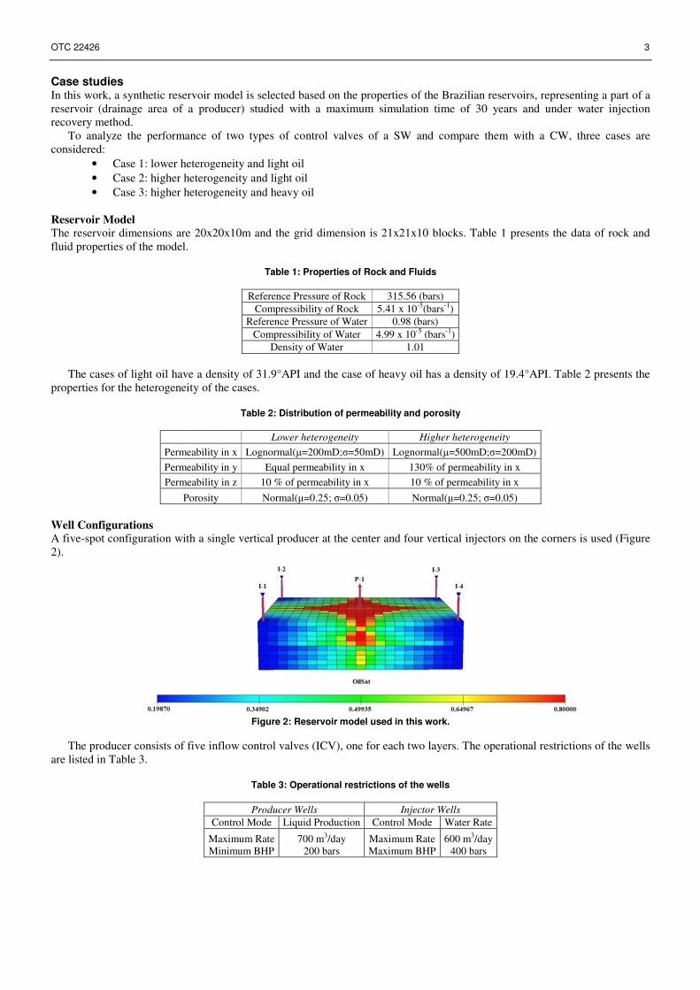
A five-spot configuration with a single vertical producer at the center and four vertical injectors on the corners is used (Figure 2).

Figure 2: Reservoir model used in this work.

The producer consists of five inflow control valves (ICV), one for each two layers. The operational restrictions of the wells are listed in Table 3.

Table 3: Operational restrictions of the wells

Producer Wells Injector Wells

Control Mode Liquid Production Control Mode Water Rate

Maximum Rate 700 m3/day Maximum Rate 600 m3/day Minimum BHP 200 bars Maximum BHP 400 bars

4 OTC 22426

For injectors, the maximum rate of water injection is equivalent to the fluid production volume, considering reservoir conditions to avoid high pressurization.

Evolutionary Algorithm Parameters

Table 4 presents the evolutionary algorithm parameters used in each type of control. There is only one variable for both the CW and the SW with reactive control and five variables for the SW with proactive control.

Table 4: Evolutionary algorithm parameters

Conventional

Wells Smart Wells:

Reactive Control Smart Wells:

Proactive Control

Number of Generations 20 20 50

Size of Population 10 10 40

Number of Elite Individuals 3 3 3

Crossover Rate 0.8 0.8 0.8

Economic Scenarios

To analyze the valve’s operation by two controls of the SW and the CW under economic uncertainty, three economic scenarios are considered: pessimistic, probable and optimistic. The values for each scenario are shown in Table 5.

Table 5: Economic data

Economic Scenarios

Discount Rate (% p.a.)

Oil Price (US$/bbl)

Oil Production Cost (US$/bbl)

Water Production Cost (US$/bbl)

Water Injection Cost (US$/bbl)

Optimistic 8.8 65.00 8.00 0.70 1.00

Probable 8.8 50.00 8.00 1.00 1.00

Pessimistic 8.8 35.00 8.00 1.50 1.00

The economic base model is selected following a simplified Brazilian fiscal regime, assuming the data presented in Table 6.

Table 6: Economic parameters used in a simplified Brazilian fiscal regime

Economic parameter Value

Corporate tax 25%

Royalties 10%

Social contribution 9%

Linear Depreciation (years) 10

In all cases, the present value is discounted by the investment value of US$ 70 million, corresponding to the sum of the

investments in the platform, drilling of conventional wells and cost of abandonment. This relatively low value is proportional to the investment that would be made in a field with several wells, i.e., an estimated value considering this model as a sector of a field.

In the economic analysis of this work, just the investments in the CW are considered, not including the investments in smart completion (packers, flat-packs, valves and sensors). To assess the feasibility of using the SW, the differences in NPV between the CW and the SW are considered for each case, determining the economic limit available to be used in this technology (additional costs of the SW are not considered in the NPV calculation). Results and Discussions Case 2, a more heterogeneous model and light oil, is presented here with more details, because it is the case in which the SW presents better performance than the other cases, making it interesting to show the results. The main results will be presented for the remaining cases. It should be noted that all operational parameters are kept fixed in all cases, not being part of the optimization process.

Probable Economic Scenario of Case 2

Table 7 shows the results obtained for the optimization of CW and SW. It can be seen that SW are able to increase oil production and NPV when compared to the CW, while reducing water production in both controls, proactive and reactive. Water production is an important factor in offshore fields because of the need to do the water treatment, becoming extremely important since it reduces water production, as well as increasing oil production. The differences between the NPV of SW and CW are also presented to evaluate the revenue available to be invested in smart completion and still be advantageous to use this more costly completion.

OTC 22426 5

Table 7: Results of production for CW and SW.

Probable Scenario

Oil Production (106 std m3)

Water Production (106 std m3)

Water Injection (106 std m3)

NPV (US$ millions)

∆ NPV (US$ millions)

Conventional 1.57 1.49 3.60 53.40 0

Smart - Reactive 1.59 1.47 3.61 54.56 1.16

Smart - Proactive 1.59 1.44 3.57 54.90 1.50

Table 8 presents the percentage of different types of completion for the two types of control; SW in relation to CW. The

results show that SW are able to close valves with high water production, besides keeping others open with better relations between oil and water flow, increasing oil recovery and reducing water production and, consequently, increasing NPV. For SW with reactive control, the valves are closed at different times, but all with the same optimal WCUT, maximizing the NPV of the field. In the proactive control, valves performed proactively in relation to each other, because valves which started to decrease NPV closed the completion to increase revenue in other valves of the well.

Table 8: Differences in indicators for SW in relation to CW.

Probable Scenario Oil Production Water Production Water Injection NPV

Smart - Reactive + 1.33 % - 1.44 % + 0.20 % + 2.12 %

Smart - Proactive + 1.21 % - 3.98 % - 1.03 % + 2.73 %

Figure 3(a) and (b) show the results of SW production with the two controls acting jointly with the results of the CW. The

time at which the valves close can be observed them, and consequently, the time at which there is an increase in oil production and a drop in water production rates, symmetrically, in two curves. As can be seen, proactive control provides a greater reduction in water production than reactive control.

(a)

(b)

Figure 3: Production of two types of control valves of smart and conventional wells. (a) reactive; (b) proactive.

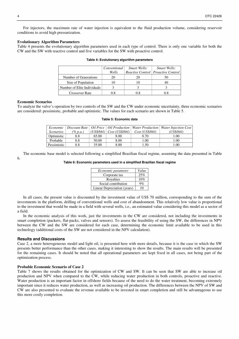
Figure 4 highlights the time at which each valve closes in the SW and the time at which the CW closes. It can be seen that the last layers, with higher permeability, are the layers whose valves close first, since the water comes before these valves. On the other hand, as the CW does not have valves, it is not possible to detect water production in different regions of the well. Because it cannot respond appropriately to the increase in oil production and to the decrease in water production, it cannot seek better relations between oil and water flows.

Another important observation in the graph is the closure of neighbor valves at the same time, showing that the use of two valves are unnecessary, justifying the use of just one valve with the same area of action, which would lead to cost savings of one valve. In reactive control, this occurred with the first two valves. In the case of proactive control, the last three valves are also closed at nearly the same time, indicating the feasibility of replacing those three valves with a single one, which would also generate the economy of two valves.

6 OTC 22426

Figure 4: Closing valves for SW and CW.

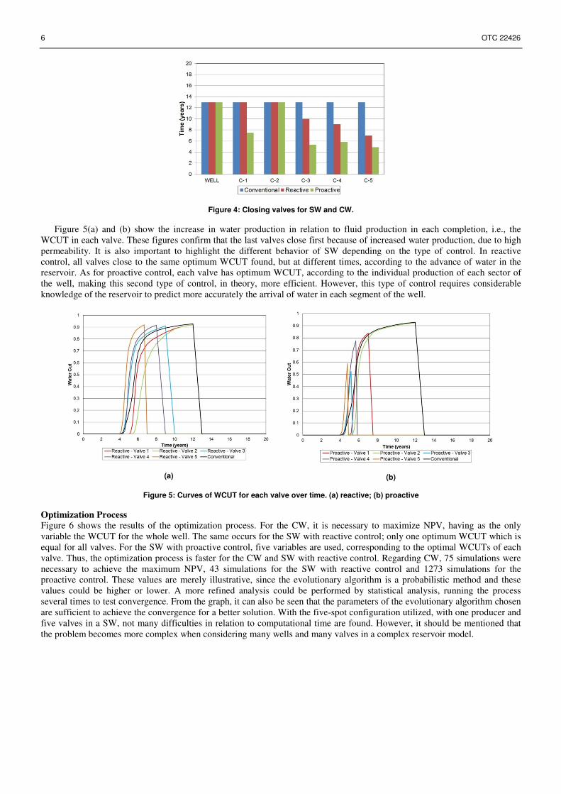
Figure 5(a) and (b) show the increase in water production in relation to fluid production in each completion, i.e., the WCUT in each valve. These figures confirm that the last valves close first because of increased water production, due to high permeability. It is also important to highlight the different behavior of SW depending on the type of control. In reactive control, all valves close to the same optimum WCUT found, but at different times, according to the advance of water in the reservoir. As for proactive control, each valve has optimum WCUT, according to the individual production of each sector of the well, making this second type of control, in theory, more efficient. However, this type of control requires considerable knowledge of the reservoir to predict more accurately the arrival of water in each segment of the well.

(a)

(b)

Figure 5: Curves of WCUT for each valve over time. (a) reactive; (b) proactive

Optimization Process

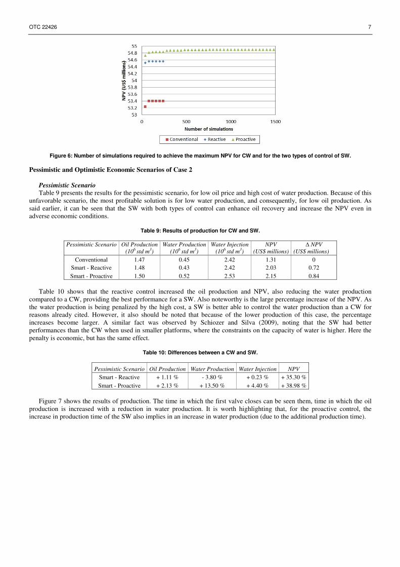
Figure 6 shows the results of the optimization process. For the CW, it is necessary to maximize NPV, having as the only variable the WCUT for the whole well. The same occurs for the SW with reactive control; only one optimum WCUT which is equal for all valves. For the SW with proactive control, five variables are used, corresponding to the optimal WCUTs of each valve. Thus, the optimization process is faster for the CW and SW with reactive control. Regarding CW, 75 simulations were necessary to achieve the maximum NPV, 43 simulations for the SW with reactive control and 1273 simulations for the proactive control. These values are merely illustrative, since the evolutionary algorithm is a probabilistic method and these values could be higher or lower. A more refined analysis could be performed by statistical analysis, running the process several times to test convergence. From the graph, it can also be seen that the parameters of the evolutionary algorithm chosen are sufficient to achieve the convergence for a better solution. With the five-spot configuration utilized, with one producer and five valves in a SW, not many difficulties in relation to computational time are found. However, it should be mentioned that the problem becomes more complex when considering many wells and many valves in a complex reservoir model.

OTC 22426 7

Figure 6: Number of simulations required to achieve the maximum NPV for CW and for the two types of control of SW.

Pessimistic and Optimistic Economic Scenarios of Case 2

Pessimistic Scenario

Table 9 presents the results for the pessimistic scenario, for low oil price and high cost of water production. Because of this unfavorable scenario, the most profitable solution is for low water production, and consequently, for low oil production. As said earlier, it can be seen that the SW with both types of control can enhance oil recovery and increase the NPV even in adverse economic conditions.


Pessimistic Scenario




NPV (US$ millions)


Conventional 1.47 0.45 2.42 1.31 0

Smart - Reactive 1.48 0.43 2.42 2.03 0.72

Smart - Proactive 1.50 0.52 2.53 2.15 0.84

Table 10 shows that the reactive control increased the oil production and NPV, also reducing the water production

compared to a CW, providing the best performance for a SW. Also noteworthy is the large percentage increase of the NPV. As the water production is being penalized by the high cost, a SW is better able to control the water production than a CW for reasons already cited. However, it also should be noted that because of the lower production of this case, the percentage increases become larger. A similar fact was observed by Schiozer and Silva (2009), noting that the SW had better performances than the CW when used in smaller platforms, where the constraints on the capacity of water is higher. Here the penalty is economic, but has the same effect.

Table 10: Differences between a CW and SW.

Pessimistic Scenario Oil Production Water Production Water Injection NPV

Smart - Reactive + 1.11 % - 3.80 % + 0.23 % + 35.30 %

Smart - Proactive + 2.13 % + 13.50 % + 4.40 % + 38.98 %

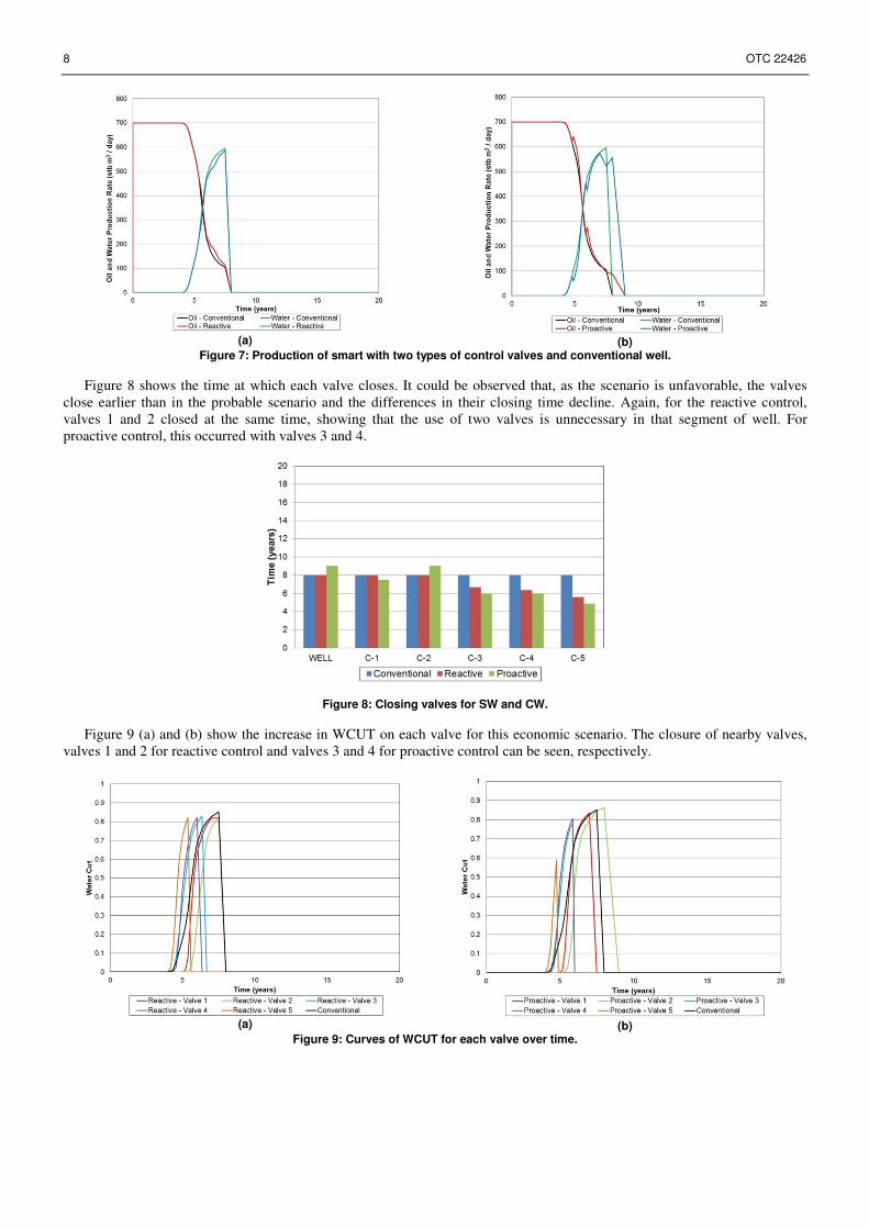
Figure 7 shows the results of production. The time in which the first valve closes can be seen them, time in which the oil

production is increased with a reduction in water production. It is worth highlighting that, for the proactive control, the increase in production time of the SW also implies in an increase in water production (due to the additional production time).

8 OTC 22426

(a)

(b)

Figure 7: Production of smart with two types of control valves and conventional well.

Figure 8 shows the time at which each valve closes. It could be observed that, as the scenario is unfavorable, the valves close earlier than in the probable scenario and the differences in their closing time decline. Again, for the reactive control, valves 1 and 2 closed at the same time, showing that the use of two valves is unnecessary in that segment of well. For proactive control, this occurred with valves 3 and 4.


Figure 9 (a) and (b) show the increase in WCUT on each valve for this economic scenario. The closure of nearby valves, valves 1 and 2 for reactive control and valves 3 and 4 for proactive control can be seen, respectively.

(a)

(b)

Figure 9: Curves of WCUT for each valve over time.

OTC 22426 9

Optimistic Scenario

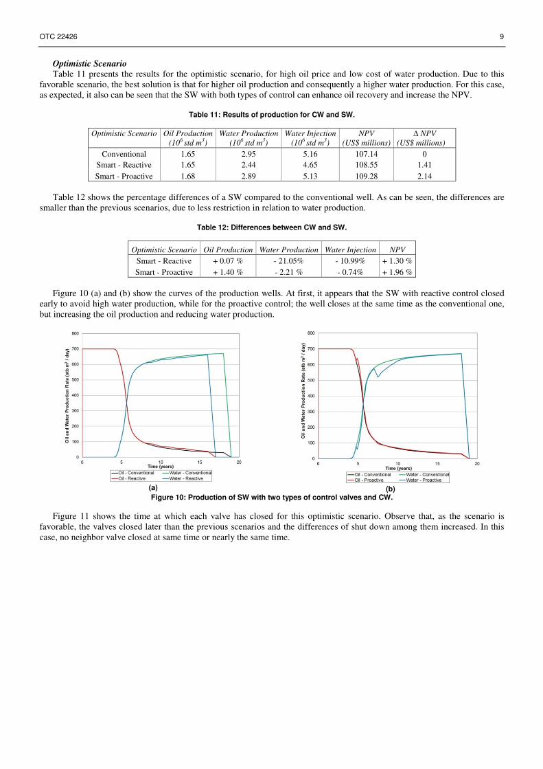
Table 11 presents the results for the optimistic scenario, for high oil price and low cost of water production. Due to this favorable scenario, the best solution is that for higher oil production and consequently a higher water production. For this case, as expected, it also can be seen that the SW with both types of control can enhance oil recovery and increase the NPV.


Optimistic Scenario




NPV (US$ millions)


Conventional 1.65 2.95 5.16 107.14 0

Smart - Reactive 1.65 2.44 4.65 108.55 1.41

Smart - Proactive 1.68 2.89 5.13 109.28 2.14

Table 12 shows the percentage differences of a SW compared to the conventional well. As can be seen, the differences are

smaller than the previous scenarios, due to less restriction in relation to water production.

Table 12: Differences between CW and SW.

Optimistic Scenario Oil Production Water Production Water Injection NPV

Smart - Reactive + 0.07 % - 21.05% - 10.99% + 1.30 %

Smart - Proactive + 1.40 % - 2.21 % - 0.74% + 1.96 %

Figure 10 (a) and (b) show the curves of the production wells. At first, it appears that the SW with reactive control closed

early to avoid high water production, while for the proactive control; the well closes at the same time as the conventional one, but increasing the oil production and reducing water production.

(a)

(b)

Figure 10: Production of SW with two types of control valves and CW.

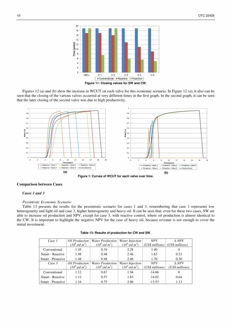
Figure 11 shows the time at which each valve has closed for this optimistic scenario. Observe that, as the scenario is favorable, the valves closed later than the previous scenarios and the differences of shut down among them increased. In this case, no neighbor valve closed at same time or nearly the same time.

10 OTC 22426


Figures 12 (a) and (b) show the increase in WCUT on each valve for this economic scenario. In Figure 12 (a), it also can be seen that the closing of the various valves occurred at very different times in the first graph. In the second graph, it can be seen that the later closing of the second valve was due to high productivity.

(a)

(b)

Figure 1: Curves of WCUT for each valve over time.

Comparison between Cases

Cases 1 and 3

Pessimistic Economic Scenario Table 13 presents the results for the pessimistic scenario for cases 1 and 3, remembering that case 1 represents low

heterogeneity and light oil and case 3, higher heterogeneity and heavy oil. It can be seen that, even for these two cases, SW are able to increase oil production and NPV, except for case 3, with reactive control, where oil production is almost identical to the CW. It is important to highlight the negative NPV for the case of heavy oil, because revenue is not enough to cover the initial investment.


Case 1




NPV (US$ millions)


Conventional 1.45 0.34 2.28 1.40 0

Smart - Reactive 1.48 0.48 2.46 1.63 0.23

Smart - Proactive 1.48 0.48 2.46 1.70 0.30

Case 3




NPV (US$ millions)


Conventional 1.12 0.67 1.94 -14.66 0

Smart - Reactive 1.12 0.57 1.83 -14.02 0.64

Smart - Proactive 1.16 0.75 2.06 -13.53 1.13

OTC 22426 11

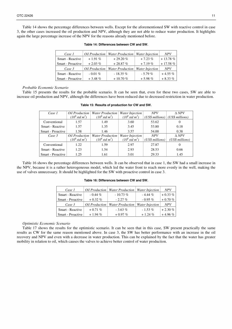
Table 14 shows the percentage differences between wells. Except for the aforementioned SW with reactive control in case 3, the other cases increased the oil production and NPV, although they are not able to reduce water production. It highlights again the large percentage increase of the NPV for the reasons already mentioned before.


Case 1 Oil Production Water Production Water Injection NPV

Smart - Reactive + 1.91 % + 29.20 % + 7.23 % + 13.78 %

Smart - Proactive + 2.03 % + 28.87 % + 7.19 % + 17.58 %


Smart - Reactive - 0.01 % - 18.35 % - 5.79 % + 4.55 %

Smart - Proactive + 3.48 % + 10.70 % + 5.98 % + 8.33 %

Probable Economic Scenario Table 15 presents the results for the probable scenario. It can be seen that, even for these two cases, SW are able to

increase oil production and NPV, although the differences have been reduced due to decreased restriction in water production.


Case 1




NPV (US$ millions)


Conventional 1.57 1.49 3.60 53.62 0

Smart - Reactive 1.57 1.35 3.45 53.80 0.18

Smart - Proactive 1.58 1.46 3.57 54.00 0.38

Case 3




NPV (US$ millions)


Conventional 1.22 1.59 2.97 27.87 0

Smart - Reactive 1.23 1.54 2.93 28.53 0.66

Smart - Proactive 1.25 1.61 3.01 29.33 1.45

Table 16 shows the percentage differences between wells. It can be observed that in case 1, the SW had a small increase in the NPV, because it is a rather heterogeneous model, which led the water front to reach more evenly in the well, making the use of valves unnecessary. It should be highlighted for the SW with proactive control in case 3.



Smart - Reactive - 0.44 % - 10.73 % - 4.44 % + 0.33 %

Smart - Proactive + 0.32 % - 2.27 % - 0.95 % + 0.70 %


Smart - Reactive + 0.71 % - 3.63 % - 1.53 % + 2.30 %

Smart - Proactive + 1.94 % + 0.97 % + 1.24 % + 4.96 %

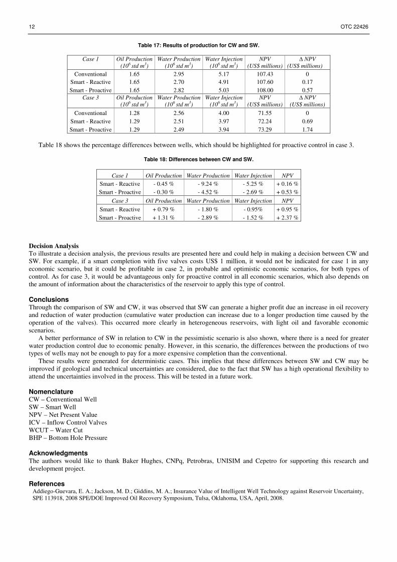
Optimistic Economic Scenario Table 17 shows the results for the optimistic scenario. It can be seen that in this case, SW present practically the same

results as CW for the same reason mentioned above. In case 3, the SW has better performance with an increase in the oil recovery and NPV and even with a decrease in water production. This can be explained by the fact that the water has greater mobility in relation to oil, which causes the valves to achieve better control of water production.

12 OTC 22426


Case 1




NPV (US$ millions)


Conventional 1.65 2.95 5.17 107.43 0

Smart - Reactive 1.65 2.70 4.91 107.60 0.17

Smart - Proactive 1.65 2.82 5.03 108.00 0.57

Case 3




NPV (US$ millions)


Conventional 1.28 2.56 4.00 71.55 0

Smart - Reactive 1.29 2.51 3.97 72.24 0.69

Smart - Proactive 1.29 2.49 3.94 73.29 1.74

Table 18 shows the percentage differences between wells, which should be highlighted for proactive control in case 3.



Smart - Reactive - 0.45 % - 9.24 % - 5.25 % + 0.16 %

Smart - Proactive - 0.30 % - 4.52 % - 2.69 % + 0.53 %


Smart - Reactive + 0.79 % - 1.80 % - 0.95% + 0.95 %

Smart - Proactive + 1.31 % - 2.89 % - 1.52 % + 2.37 %

Decision Analysis

To illustrate a decision analysis, the previous results are presented here and could help in making a decision between CW and SW. For example, if a smart completion with five valves costs US$ 1 million, it would not be indicated for case 1 in any economic scenario, but it could be profitable in case 2, in probable and optimistic economic scenarios, for both types of control. As for case 3, it would be advantageous only for proactive control in all economic scenarios, which also depends on the amount of information about the characteristics of the reservoir to apply this type of control. Conclusions Through the comparison of SW and CW, it was observed that SW can generate a higher profit due an increase in oil recovery and reduction of water production (cumulative water production can increase due to a longer production time caused by the operation of the valves). This occurred more clearly in heterogeneous reservoirs, with light oil and favorable economic scenarios.

A better performance of SW in relation to CW in the pessimistic scenario is also shown, where there is a need for greater water production control due to economic penalty. However, in this scenario, the differences between the productions of two types of wells may not be enough to pay for a more expensive completion than the conventional.

These results were generated for deterministic cases. This implies that these differences between SW and CW may be improved if geological and technical uncertainties are considered, due to the fact that SW has a high operational flexibility to attend the uncertainties involved in the process. This will be tested in a future work. Nomenclature CW – Conventional Well SW – Smart Well NPV – Net Present Value ICV – Inflow Control Valves WCUT – Water Cut BHP – Bottom Hole Pressure Acknowledgments The authors would like to thank Baker Hughes, CNPq, Petrobras, UNISIM and Cepetro for supporting this research and development project. References

Addiego-Guevara, E. A.; Jackson, M. D.; Giddins, M. A.; Insurance Value of Intelligent Well Technology against Reservoir Uncertainty, SPE 113918, 2008 SPE/DOE Improved Oil Recovery Symposium, Tulsa, Oklahoma, USA, April, 2008.

OTC 22426 13

Baeck, T.; Fogel, D.B.; Michalewicz, Z.; Evolutionary Computation. IOP Publishing, UK, 2000.

Doublet, D. C.; Aanonsen, S. I.; Tai, X. C.; An Efficient Method for Smart Well Production Optimisation. Journal of Petroleum Science and Engineering, Elsevier, Amsterdam, 69 (2009) 25 - 39.

Ebadi, F.; Davies, D. R.; Should “Proactive” or “Reactive” Control Be Chosen for Intelligent Well Management? SPE 99929, 2006 SPE Intelligent Energy Conference and Exhibition, Amsterdam, Netherlands, April, 2006.

Emerick, A. A.; Portella, R. C. M.; Production Optimization with Intelligent Wells. SPE 107261, 2007 SPE Latin American and Caribbean Petroleum Engineering Conference, Buenos Aires, Argentina, 2007.

Kharghoria, A.; Zhang, F.; LI, R., Jalali, Y.; Application of Distributed Electrical Measurements and Inflow Control in Horizontal Wells under Bottom-Water Drive. SPE 78275, 2002 SPE 13th European Petroleum Conference, Aberdeen, Scotland, October, 2002.

Sarma, P.; Aziz, K.; Durlofsky, L. J.; Implementation of Adjoint Solution for Optimal Control of Smart Wells. SPE 92864, 2005 SPE Reservoir Simulation Symposium, Houston, Texas, USA, February, 2005.

Schiozer, D. J.; Silva, J. P.Q. G.; Methodology to Compare Smart and Conventional Wells. SPE 124949, 2009 SPE Annual Technical Conference and Exhibition, New Orleans, USA, October, 2009.

Su, H. J., Smart Well Production Optimization Using an Ensemble-Based Method. SPE 126072, 2009 SPE Saudi Arabia Section Technical Symposium and Exhibition, Alkohobar, Saudi Arabia, May, 2009.

Van Essen, G. M.; Jansen, J. D.; Brouwer, D. R.; Douma, S. G.; Rollett, K. I.; Harris, D. P.; Optimization of Smart Wells in the St. Joseph Field. SPE 123563, 2009 SPE Asia Pacific Oil and Gas Conference and Exhibition, Jakarta, Indonesia, August, 2009.

Yeten, B.; Durlofsky, L. J.; Aziz, K.; Optimization of Smart Well Control. SPE 79031, 2002 SPE/PS-CIM/CHOA International Thermal Operations and Heavy Oil Symposium and International Horizontal Well Technology Conference, Calgary, Alberta, Canada, 2002.

Yeten, B.; Brouwer, D. R; Durlofsky, L. J.; Aziz, K.; Decision Analysis under Uncertainty for Smart Well Deployment, Journal of Petroleum Science & Engineering, Elsevier, Amsterdam, 43 (2004) 183 -19.

otc 22426 comparison between smart and conventional wells

Documents