organically linked iron oxide nanoparticle supercrystals ... · supercrystals with exceptional...
TRANSCRIPT

1
Supplementary Information (SI) Organically linked iron oxide nanoparticle supercrystals with exceptional isotropic mechanical properties Axel Dreyer1, Artur Feld2, Andreas Kornowski2, Ezgi D. Yilmaz1, Heshmat Noei3, Andreas Meyer2, Tobias Krekeler4, Chengge Jiao5, Andreas Stierle3,6, Volker Abetz2,7, Horst Weller2,8,9 and Gerold A. Schneider1* 1Institute of Advanced Ceramics, Hamburg University of Technology, Denickestrasse 15, D-‐21073 Hamburg, Germany 2Institute of Physical Chemistry, Hamburg University, Grindelallee 117, D-‐20146 Hamburg, Germany 3DESY NanoLab, Deutsches Elektronensynchrotron DESY, Notkestrasse 85, D-‐22607 Hamburg, Germany 4Electron Microscopy Unit, Hamburg University of Technology, Eißendorfer Str. 42, D-‐21073 Hamburg 5FEI Company, Achtseweg Noord 5, 5651 GG, Eindhoven, the Netherlands 6Physics Department, Hamburg University, Jungiusstrasse 11, D-‐20355 Hamburg, Germany 7Institute of Polymer Research, Helmholtz-‐Zentrum Geesthacht, Max-‐Planck-‐Strasse 1, 21502 Geesthacht, Germany 8Center for Applied Nanotechnology, Grindelallee 117, D-‐20146 Hamburg 9Department of Chemistry, Faculty of Science, King Abdulaziz University, Jeddah, Saudi Arabia *e-‐mail: [email protected] 1. Particle synthesis Magnetite nanocrystals were synthesized in accordance to Yu et al.1, briefly, a mixture of 12.40 g FeO(OH) (0.139 mol), 294.0 g oleic acid (1.04 mol) and 500 g 1-‐octadecene was heated under nitrogen at 320 °C for 2 hours. After synthesis the particles were precipitated by adding acetone, centrifuged and stored in toluene. Several batches were synthesized, which differ slightly in size. From a size histogram of 800 particles of the here exemplarily shown TEM images a mean diameter of 15.4±0.8 nm was determined. SAED patterns (Figure 2, see also SI chap. 3) are in accord to magnetite reference. To obtain the bulk solid material the particles were precipitated with acetone and redispersed in tetrahydrofuran by ultrasonication and subsequently poured into a sealed die resulting in sedimentation and self-‐assembly.
Figure SI 1 | TEM images of the primary oleic acid stabilized iron oxide nanoparticles, which were used for the experiments.
Organically linked iron oxide nanoparticle supercrystals with exceptional isotropic mechanical properties
SUPPLEMENTARY INFORMATIONDOI: 10.1038/NMAT4553
NATURE MATERIALS | www.nature.com/naturematerials 1

2
2. SAXS Measurements Small angle X-‐ray scattering (SAXS) measurements were performed with the powdered samples to determine the arrangement of the iron oxide nanoparticles in the composite. An Incoatec™ X-‐ray source IµS with Quazar Montel optics and a focal spot diameter at sample of 700 µm with a wavelength of 0.154 nm was used. The distance between sample and detector was 1.6 m (CCD-‐Detector Rayonix™ SX165). The uniform pestled sample powders were applied in a thin layer onto scotch tape and measured in transmission geometry. The measurement time per sample was 600 s. The analysis was performed with the software Scatter2,3. The lattice type of the arrangement is fcc for all temperatures. The nearest neighbor distance (nnd) becomes smaller with increasing temperature. Assuming a spherical form factor for the particles, the particles may have partially contact above 350 °C, as the nnd becomes smaller than the measured diameter (16.0 nm) of the iron oxide core. If the particles get faceted with increasing temperature, it is possible that there is still a thin organic layer between them. Above 350 °C, the particles starts to sinter and the nnd is significantly smaller than the particle diameter. Also, the polydispersity of the particles increases from 4.5 % at 150 °C to 10 % at 450 °C and in the meantime the quality of order of the arrangement decreases, as one can observe by broadening and the missing higher orders of the crystalline reflections.
Additionally, SAXS of the initial particle solution was made, to determine the particle form factor and diameter in solution. The strong and clearly oscillating spherical form factor allowed us to calculating the average diameter of the iron oxide particles with oleic acid shell very precisely to 16.2 nm with a standard deviation of 6 %.
Figure SI 2 | SAXS of iron oxide/oleic acid in solution (left) and as nanocomposite at different temperatures (right).
Figure SI 3 | Structural SAXS results of iron oxide/oleic acid nanocomposite at different temperatures.

3
To determine the orientation of iron oxide/oleic acid supercrystals in the nanocomposite small angle X-‐ray scattering (SAXS) measurements were performed with pestled samples and the bulk material. These grazing incidence SAXS (GISAXS) measurements give information about the orientation distribution of the iron oxide/oleic acid supercrystals within the millimeter-‐sized bulk samples. A typical semi-‐circular GISAXS halfring-‐pattern for our samples is shown in Figure SI 4 and reveals a uniform and isotropic spherical form factor scattering. The fcc-‐superlattice reflections are statistically distributed in the azimuthal direction, indicative of a random orientation of supercrystals. The few bright spots within the diffuse ring-‐like pattern are generated by significantly larger supercrystals than the average supercrystal size. The GISAXS reflections have the same broadening as the ones from the pestled sample and the calculated crystalline domain sizes have diameters of about 100 nm. Statistically, this means that there exist a lot of approx. 100 nm sized supercrystalline domains inside the supercrystals.
Figure SI 4 | GISAXS detector pattern of iron oxide/oleic acid sample annealed at 250°C. The solid workpiece was measured under grazing incidence with an angle of incidence of 0.2°. The x-‐y-‐scale of the pattern is q (nm-‐1). The scattering horizon at qy=0.15nm
-‐1 is clearly visible. Arising reflections below the horizon were generated at the edges of the relatively rough sample, which leads to additional SAXS scattering.
3. SEM, TEM and SAED Measurements TEM and HRTEM measurements were carried out on a JEOL JEM 1011 at 100kV and on a JEOL JEM 2200 FS at 200kV equipped with two CEOS Cs correctors (CETCOR, CESCOR) and a Gatan 4K UltraScan 1000 camera. To investigate the nanoparticles a drop of the diluted colloidal solution was deposited on a carbon coated 400 mesh TEM grid. The excess of solvent was removed with a filter paper and the grid was air dried. The compressed and heated samples were crushed into fine powder with a mortar and pestle. The powder was suspended in toluene and one drop of this suspension was deposited on the carbon coated TEM grid. The excess of solvent was removed with a filter paper and the grid was dried under air. SEM investigations were carried out on a LEO 1550 SEM at 20kV. The

4
same powder as for the TEM measurements was fixed on adhesives carbon pads on standard SEM specimen holder.
Figure SI 5 | SAED measurements of the pressed nanocomposites at different temperatures heated samples. TEM images of the selected area (left) and the corresponding rotation profiles (right) of the electron diffraction (inset). The crystal structures magnetite is labeled with blue bars in the lower rotation profile. The electron diffraction patterns clearly indicate that over the whole treatment process no phase transition of the inner crystal structure of the individual nanoparticles occur (Figure SI 5). In addition no preferred crystallographic orientation of the nanoparticles to each other is observable. Comparing the appearance and the intensity distribution of the diffraction rings at different temperatures gives no indications for a change of the arrangement or for significant bulk aggregation of the nanoparticles. These findings are also supported by SEM and TEM investigation of the crushed samples (Figure SI 6). The slight narrowing of the diffraction rings with increasing temperature is a result of temperature-‐induced enhancement of the crystallinity of the iron oxide nanoparticles. At temperatures above 350°C a partially increased crystalline domain size arises by attaching of well faceted adjacent nanoparticles which are aligned in the same crystallographic direction.

5
Figure SI 6 | SEM images of the compressed and at different temperatures heated samples (left), TEM (middle) and HRTEM images (right) of the same samples. All images (SEM and TEM as well) show clearly the appearance of individual nanoparticles at all stages of the sample treatments.

6
4. Determination of the mass fraction of oleic acid The mass fraction of oleic acid was determined by thermogravimetry and He-‐pycnometry. 4.1 He-‐pycnometry Our nanocomposite consists of the mineral magnetite (Fe3O4) with density ρFO = 5.24 g·∙cm-‐³ and the organic oleic acid (OA: C18H34O2) with density ρOA = 0.89 g·∙cm-‐³ and the solvent where we assume the same density as for the oleic acid ρSol = 0.89 g·∙cm-‐³. Both densities are denoted as ρOR. The densities of the magnetite and oleic acid were determined at 25 °C4. The mass fraction wOR of adsorbed oleic acid molecules on the surface of the magnetite is defined as:
)25()25()25(CmCmCw
NC
OROR °
°=° (1)
where mOR(25°C) is the mass of the oleic acid in the per nanocomposite (NC) with mNC(25 °C). The mass fraction wOR can be calculated as follows: As there is open porosity between the fcc ordered spherical magnetite particles He-‐gas enters completely inside the nanocomposite. Hence the He-‐pycnometry measures the density of the magnetite particles together with their organic film, ρNC. As a consequence the adsorbed organic mass fraction wOR can be calculated from the measured ρPY by He-‐pycnometric density (Accu Pyc II 1340, Micromeritics) as:
wOR (25°C) =ρOR (ρPY − ρFO )ρPY (ρOR − ρFO )
(2)
For the pycnometric measurements the nanocomposite was ground in a mortar to fine powder and ~0.35 g were weighed in a 1cm3 measuring cell. After 100 purification cycles the 75 measuring cycles gave von ρNC=3.567±0.016 g·∙cm-‐³. With (2) the mass fraction of oleic acid at 25 °C is wOR(25 °C)=0.096±0.001. 4.2 Thermogravimteric analysis (TGA) The nanocomposite consists of thermally stable magnetite (Fe3O4, mp: >1500 °C) and volatile oleic acid (OA: C18H34O2, bp: 360 °C) and the volatile solvent. The measured TGA-‐values are all normalized to the original weight:
)25()25(0 CmCmmm OASolNP °+°+= (3) where mNP is the mass of the magnetite nanoparticles, mSol the mass of the solvent and mOA the mass of the oleic acid all at room temperature. As the mass of the magnetite particles stays constant up to 400°C we do not take the temperature dependence for magnetite into account. FTIR-‐spectroscopy at the desorbed gases detects the blowout of solvent residues between 50 °C and 150 °C. Therefore we relate the mass loss up to 150°C only to the solvent and hence at 150°C the measured weight fraction wm is:
0
)150(m
Cmw Solm
°Δ= (4)

7
We want to determine the weight fraction of the oleic acid wOA :
)()()(Tmm
TmTwOANP
OAOA +
= (5)
As we identify
)25()150( CmCm Sol °=°Δ (6) together with (4) and (1) we get:
))25(1(0 Cwmm ORNP °−= (7) Also there is no oleic acid desorption up to 150°C and therefore:
)25()150( CmCm OAOA °=° (8) Together with (1,3,4,6) we get:
))150()25(()25( 0 CwCwmCm mOROA °−°=° (9) which gives together with (1,5,7):
087.09896.00856.0
)150(1)150()25()150(
==
°−
°−°=°
CwCwCwCw
m
mOROA
(10)
(values are taken from Table SI 1) For temperatures between 150°C and 400°C FTIR detects the desorption of oleic acid, hence in this temperature range:
00
)()25()()(m
TmCmmTmTw OAOAOA
m−°
=Δ
= (11)
Introducing (11) together with (7) into (5) gives:
)(9896.0)(0856.0
)()150(1)()150()25()(
TwTw
TwCwTwCwCwTw
m
m
mm
mmOROA
−−
=
−°−−°−°
=
(12)
(values are taken from Table SI 1)

8
5. Surface density of oleic acid on the particle surface TEM investigations of 718 spherical magnetite particles gave a diameter d=17.6±1.6 nm for these investigations. This differs from the nanoparticle size in chap. 1 but we assume that calculated surface density is not much influenced by a slightly different particle diameter but otherwise identical processing. The specific surface A -‐ the surface area per mass of a particle -‐ of the magnetite nanoparticles coated with oleic acid is defined as:
NC
P
mAA = (13)
The surface area of a spherical particle with diameter d is:
2dAP π= (14) and the mass of the nanocomposite particle consisting of the iron oxide with adsorbed oleic acid is
NCNCdm ρπ6
3
= (15)
Hence we get:
dA
NCρ6
= (16)
For our nanoparticles this results in A=95.7±9.2 m²·∙g-‐1. The surface density of oleic acid particles on the surface of the spherical iron oxide is defined as:
2dNOA
OA πρ = (17)
where NOA is the absolute number of oleic acid molecules in a monolayer on the iron oxide nanoparticle surface. Here we assume that only a monolayer of oleic acid is present, which is confirmed by the final result. The mass of the monolayer of oleic acid particles is:
A
OAOAOA NMNm = (18)
with the molar mass of of oleic acid MOA and the Avogadro number NA. Together with (13,4,17,18) we finally get for the surface density of oleic acid molecules:
AMNTw
AmMNTm
dTNT
OA
AOA
NC
OA
AOA
OAOA )(
)()()( 2 =
⎟⎟⎠
⎞⎜⎜⎝
⎛
==π
ρ (19)
Here we explicitely introduced the temperature T dependence. With the molar mass of oleic acid, MOA=282 g/mol, and the Avogadro number, 6.022 1023 mol-‐1, we get:

9
22
2313.22
7.95282
110 6
nmgm
molg
molAM
N
oA
A =×
=
(20)
Table SI 1 | Measured temperature T dependent fractional mass reduction wm of the iron oxide/oleic acid nanocomposite measured by TGA. From this data, the oleic acid mass fraction wOA and surface density ρOA were calculated according to equations (10), (12) and (19).
T / °C wm= (∆m(T)/m) / % WOA / % ρOA / nm-‐²
150 1.040 8.7 1.91 200 1.615 7.1 1.58 250 2.427 6.4 1.43 300 3.388 5.4 1.20 350 5.259 3.5 0.78 400 7.266 1.4 0.31
6. Energy of carboxylate bond to metal ions As far as we know, accurate values for the binding energy of carboxylic acid to iron oxide have yet to be reported in the literature. To this end, we analyzed our thermograms (Figure 3a) by a combination of the Habenschaden-‐Küppers method5 and the Redhead method6 to obtain an estimate for the bond energy. We determine the kinetic pre-‐exponential factor of the desorption process with 2.5·∙108 s-‐1 by the Habenschaden-‐Küppers method5 and use this value for the Redhead-‐analysis6. Hereby, we obtain activation energies of 1.0 eV and 1.3 eV for the desorption peaks at 230 °C and 350 °C. These estimates fall into the range of known binding energies of formic acid on TiO2(101) and ZnO(10-‐10) of 0.92 eV 7 and 1.38 eV to 1.86 eV 8, respectively. Hence the binding energy of a covalent C-‐C bond (3.6 eV) is much stronger than the carboxylate bond of the oleic acid COOH-‐group to the iron oxide surface. As a consequence the molecular chain between two iron oxide nanoparticles will break at the carboxylate bond. 7. Infrared Spectroscopy (IR) 7.1 Attenuated total reflection (ATR) -‐ Infrared spectroscopy (IR) A high coverage and interpenetration of the organic molecules on particle surfaces leads to a limitation of the conformational freedom of their alkyl chains. The IR spectroscopy gives information about this decrease9,10. It is well known from literature, that the symmetric and asymmetric CH-‐stretching vibrations shifts to smaller wave numbers for immobile alkyl systems from 2855 cm-‐1 to 2850 cm-‐1 for the symmetric vibration and from 2924 cm-‐1 to 2920 cm-‐1 for the asymmetric vibration11. Figure SI 7 shows the IR spectra of iron oxide/oleic acid particles solved in carbon tetrachloride and dried. As reference, oleic acid was also measured in carbon tetrachloride solution and pure. All samples were investigated as a film on a diamond ATR crystal Brucker Platinum Alpha.

10
Figure SI 7 | ATR-‐FTIR measurement of oleic acid (OA) in carbon tetrachloride (CCl4) solution and pure as a liquid as well as magnetite particles coated with oleic acid (Fe3O4@OA) in CCl4 solution and dried as a solid. The shift of the symmetric and asymmetric CH-‐stretching vibrations to smaller wave numbers indicates a limitation of the conformational freedom of the alkyl chains. The highest conformational flexibility has the free oleic acid molecules in solution. An adsorption to a iron oxide particle surface limits their flexibility, which is now comparable with that in pure oleic acid. By removal of the solvent and the consequential particle aggregation reduces additionally the alkyl flexibility. The resulting immense shift and loss of conformational freedom, respectively, is comparable with that can be observed at the oleic acid crystallization12. This indicates in our point of view, a dense oleic acid layer around the particles and a significant interpenetration of these organic layers. 7.2 Ultra-‐high vacuum (UHV) -‐ Infrared reflection absorption spectroscopy (IRRAS) The UHV-‐IRRAS studies were performed at an UHV-‐system equipped IR spectrometer Bruker Vertex 80v. The IR-‐spectrometer is coupled to the UHV-‐chamber via differentially pumped KBr-‐windows. Each IR spectrum was accumulated of 1024 scans with a resolution of 2 cm-‐1 and was taken at grazing incidence (80°) at a base pressure of 9·∙10-‐10 mbar. The oleic acid functionalized Fe3O4-‐particles were stabilized on the Si wafer for UHV-‐IRRAS spectroscopy studies. A pure silicon wafer was used as reference sample. The IRRAS spectrum of the sample (Figure SI 8 and Fig. 3b) shows two dominant bands at 1377 and 1603 cm-‐1, characteristic for symmetric (ʋs) and asymmetric (ʋas) carboxylate (OCO) stretching modes, indicating that oleic acid is dissociated and chemisorbed to iron oxide via its oxygen atoms13–16. This is further approved by the lack of IR bands at higher than 3000 cm-‐1 and at about 1700 cm-‐1, corresponding to the carbonyl (C=O) and hydroxyl (OH) bands, respectively, originating from -‐COOH in a free oleic acid molecule. Additionally, the symmetric and asymmetric CH-‐stretching vibrations of the oleic acid adsorbed on the iron oxide surfaces are centered at 2850 cm-‐1 and 2920 cm-‐1 with a red shift to lower wavenumbers compared to the free oleic acid molecules, as it is expected for the immobile alkyl systems11.

11
2950 2900 2850 2800
νas(C-H)
νs(C-H)2920
2850
In
tens
ity
Wavenumber (cm-1)
1700 1600 1500 1400
νas(OCO)
νs(OCO)
Inte
nsity
Wavenumber (cm-1)
16031377
Figure SI 8 | UHV-‐IRRAS spectra acquired for the iron oxide/oleic acid.
8. X-‐ray photoelectron spectroscopy (XPS) -‐ Measurements XPS measurements were carried out in an ultrahigh vacuum (UHV) setup equipped with a high-‐resolution Specs PHOIBOS 150 2D-‐DLD Elevated Pressure Energy Analyzer equipped with differential pumping system. A monochromatic Al Kα X-‐ray source (1486.6 eV; anode operating at 15kV) was used as incident radiation. The base pressure in the measurement chamber was around 2·∙10-‐10 mbar. XP spectra were recorded in the fixed transmission mode. The pass energy of 20 eV was chosen, resulting in an overall energy resolution better than 0.4 eV. The binding energies were calibrated based on the graphite C 1s peak at 284.8 eV. The CASA XPS program with a Gaussian-‐Lorentzian mix function and Shirley background subtraction was employed to deconvolute the XP spectra. The peak positions were reproducible along with the fixed Lorentz to Gaussian ratio and full width at half maximum.
The XPS measurements on the overview in Figure SI 9a show the Fe 2p, O 1s and C 1s regions of the nanocomposite consisting of iron oxide coated with oleic acid. The resolved XPS are shown in Figure 3c and interpreted in the paper. To exclude graphitisation of oleic acid at elevated temperatures, the XP spectrum of pure graphite has been measured. C 1s peak of graphite shows an asymmetry peak centered at 284.4 eV, while the C 1s peaks of iron oxide/oleic acid are symmetrical and appear at higher binding energies. Based on this observation, we exclude a significant fraction of oleic acid graphitisation up to 350 °C in iron oxide / oleic acid samples (Figure SI 9b). Figure SI 9c demonstrates reduction of iron after annealing the oleic acid on iron oxide to higher than 400 °C.16,17 a) b) c)
1200 1000 800 600 400 200 0
Fe2s F1sO 2s
Fe 3p
Fe2p
In
tens
ity
973 K
623 K
573 K
Binding Energy (eV)
O 1s
O KLL
C 1s
!735 730 725 720 715 710 705
Fe 2p1/2Fe 2p3/2
Fe0
Binding Energy (eV)
Fe 2p973 K
Inte
nsity
707.2 eV
288 286 284 282
Inte
nsity
oleic acid on Fe3O4
Binding Energy (eV)
graphite
Figure SI 9 | Overview of the XPS spectrum of iron oxide coated with oleic acid at different temperatures (a). Pure graphene at room temperature (b) and expanded C1s for oleic acid on iron oxide (c).

12
9. Structural integrity of the samples after thermal treatment Thermal treatment of the macroscopic samples leads to millimeter sized cracks (Figure SI 10) and a corresponding very large reduction in macroscopic strength to 14 MPa. This may be caused by the emergence of thermal stresses or the diffusion of organic material out of the sample. Crack development will be investigated further in the future.
Figure SI 10 | 7x3x2 mm3 bending bar cut out of the pressed pellet before and after thermal treatment. The bending bar was heated up to 300 °C with 1 K/min in a nitrogen atmosphere in a muffle furnace. Fortunately, the thermal treatment of smaller nanocomposite pieces (3x3x2 mm³) proceeds without a macroscopic crack formation, making only smaller-‐sized samples suitable for analysis (Figure SI 11).
Figure SI 11 | 3x3x2 mm3 piece of a nanocomposite after thermal treatment. The nanocomposite was heated up to 300°C with 1 K/min in nitrogen atmosphere in the TGA. In this material micro-‐cantilever bars were cut by FIB. 10. Focused ion beam (FIB) sample preparation
Micro-‐cantilevers and micro-‐pillars were prepared fully automatically using a FEI Helios Nanolab 660 system using gallium ions at 30 kV. An automation recipe was created using iFast software. The rough milling currents used range from 47-‐9 nA, which was followed by a fine milling steps with the current of 430 pA. The final geometry of the representative specimens are shown in Figure SI 12 and the dimensions of all the tested specimens are given in the Table SI 2 and Table SI 3.
before thermal treatment after thermal treatment

13
Figure SI 12 | In (a) a representative of micro-‐cantilevers fabricated in this study is demonstrated. l* denotes the loaded cantilever length measured as the distance between the cantilever base and the indenter loading point marked with the red arrow. w and h are the width and height of the cantilever, respectively. A representative micro-‐pillar is shown in (b). d1, d2 and h denote the top diameter, the bottom diameter and the height of the pillars.
11. Mechanical characterization
11.1 Micro-‐cantilever bending
The micro-‐cantilever beam bending tests were performed in an Agilent Nano Indenter G200 system equipped with a Berkovich tip. Continuous stiffness measurement (CSM) option was selected to conduct the bending experiment with a constant strain target of 0.05 s-‐1. CSM allows the continuous recording of the contact stiffness S as a function of depth together with the load applied to the sample F and tip displacement δ. Stress–strain (σ-‐ε) curves calculated using the following equations:
σ microbend =12Fl*
wh2 (21)
ε =δh(l*)2
(22)
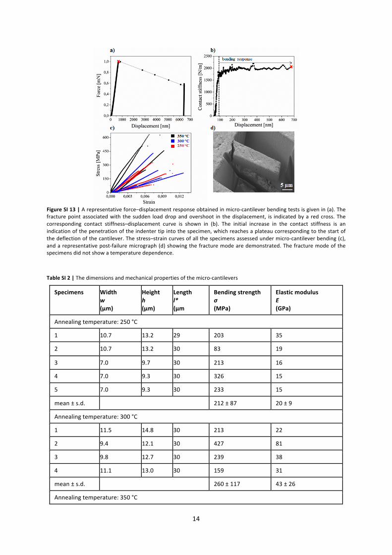
where l* is the loaded length of the cantilever, w is the width and h is the height of the cantilevers18. A typical force–displacement and contact stiffness–displacement curve obtained from the micro-‐cantilever bending tests are illustrated in Figure SI 13a and 13b. The measured displacement includes both the indentation displacement and deflection of the cantilever. During the indentation of the tip into the specimen the contact stiffness increases steadily up to the displacement point, where deflection of the cantilever starts. For the evaluation of the elastic modulus E, the stiffness is estimated by averaging the contact stiffness values between the start of the deflection and the fracture point as shown in Figure SI 13b, and inserted into the equation given below:
E = 12S(l*)2
wh3 (23)
The resultant stress–strain curves of the micro-‐cantilever tested are plotted up to the fracture point and shown in Figure SI 13c with a representative post-‐failure micrograph illustrated in Figure SI 13d. The mechanical properties such as fracture strength and elastic modulus are listed in Table SI 2.
14
Figure SI 13 | A representative force–displacement response obtained in micro-‐cantilever bending tests is given in (a). The fracture point associated with the sudden load drop and overshoot in the displacement, is indicated by a red cross. The corresponding contact stiffness–displacement curve is shown in (b). The initial increase in the contact stiffness is an indication of the penetration of the indenter tip into the specimen, which reaches a plateau corresponding to the start of the deflection of the cantilever. The stress–strain curves of all the specimens assessed under micro-‐cantilever bending (c), and a representative post-‐failure micrograph (d) showing the fracture mode are demonstrated. The fracture mode of the specimens did not show a temperature dependence. Table SI 2 | The dimensions and mechanical properties of the micro-‐cantilevers
Specimens Width w (µm)
Height h (µm)
Length l* (µm
Bending strength σ (MPa)
Elastic modulus E (GPa)
Annealing temperature: 250 °C
1 10.7 13.2 29 203 35
2 10.7 13.2 30 83 19
3 7.0 9.7 30 213 16
4 7.0 9.3 30 326 15
5 7.0 9.3 30 233 15
mean ± s.d. 212 ± 87 20 ± 9
Annealing temperature: 300 °C
1 11.5 14.8 30 213 22
2 9.4 12.1 30 427 81
3 9.8 12.7 30 239 38
4 11.1 13.0 30 159 31
mean ± s.d. 260 ± 117 43 ± 26
Annealing temperature: 350 °C

15
1 7.5 7.9 28 508 102
2 7.2 8.6 28 630 114
3 9.4 12.1 30 246 50
4 9.4 12.1 30 457 61
mean ± s.d 460 ± 160 82 ± 31
The estimated measurement errors for w and h is 0.1µm, whereas for l* it is 1µm. This leads to a 5 % error in bending strength and 11 % error in elastic modulus using Gaussian error propagation. 11.2 Micro-‐pillar compression
The micro-‐pillar compression tests were performed in an Agilent Nano Indenter G200 system equipped with a flat-‐ended punch. The diameter of the punch was 10 µm. The nanoindenter punch was positioned at the micro-‐pillar`s top surfaces using the optical microscope of the system and the specimens were loaded in CSM-‐mode with a constant strain target of 0.05 s-‐1 until fracture. Stress-‐strain curves are evaluated from the load-‐displacement data with the formulae:
σ =4Fπd1
2 (24)
ε =δh (25)
However, the measured contact stiffness reflects the combined effect of the compression of the micro-‐pillar and the indentation of the micro-‐pillar into the underlying bulk material. Applying Sneddon`s solution for a perfectly rigid cylindrical punch pressed into an elastic half-‐space, the latter should be corrected in the elastic modulus calculation19. The formula to calculate the corrected elastic modulus for a slightly tapered micro-‐pillar is adopted from20:
E = 4Shπd1d2
+(1−ν 2 )S
d2 (26)
where ν is the Possion`s ratio (0.25). S is as the maximum contact stiffness value reached in the micro-‐compression test. A typical force-‐displacement and contact stiffness–displacement curve obtained from the micro-‐pillar compression tests are shown in Figure SI 14a and 14b. The resultant stress–strain curves of the micro-‐pillars specimens are plotted up to the fracture point and shown in Figure SI 14c with a representative post-‐failure micrograph illustrated in Figure SI 14d. The mechanical properties such as fracture strength and elastic modulus are listed in Table SI 3.

16
Figure SI 14 | A representative force–displacement response obtained in micro-‐pillar compression tests is shown in (a). The fracture point associated with a large displacement burst is indicated by a red cross. The corresponding contact stiffness–displacement curve is shown in (b). The initial low stiffness values are a result of the imperfect contact between the punch and pillar surface, which eventually reach a plateau at a displacement of approx. 100 nm. (c) illustrates the stress–strain curves of all specimens assessed under micro-‐pillar compression and a representative post-‐failure micrograph showing the fracture mode is given in (d). Table SI 3 | The dimensions and mechanical properties of the micro-‐pillars
Specimens Top diameter d1 [µm]
Bottom diameter d2 [µm]
Height h [µm]
Fracture strength σ [MPa]
Elastic modulus E [GPa]
Annealing temperature: 250 °C 1 2.82 3.14 6.44 634 47 2 2.82 3.24 7.56 376 44 3 2.82 3.14 6.44 303 31 mean ± s.d. 438 ± 174 41 ± 9 Annealing temperature: 300 °C 1 2.84 3.09 7.47 515 47 2 2.84 3.16 7.47 708 47 3 2.84 3.16 7.20 1016 62 mean ± s.d. 746 ± 253 52 ± 9 Annealing temperature: 350 °C 1 2.77 3.57 5.50 610 55 2 2.77 3.47 7.81 730 69 3 2.77 3.47 7.02 659 62 4 2.77 3.47 7.58 625 62 5 2.77 3.60 7.10 1074 74 mean ± s.d. 740± 193 64 ±7 The estimated error of all length measurements is 0.1µm, which leads to a 7% error in compressive strength and 5% error in elastic modulus using Gaussian error propagation.

17
11.3 Isotropy of the mechanical properties measured by nanoindentation
As stated in Methods: Mechanical Characterization of the manuscript „5x5 arrays of indentations were performed.“ The distance of the indents was 50 µm and an area of 250x250 µm2 was probed by the indents. From SAXS and SEM measurements we can conclude that the supercrystals are randomly oriented and much smaller than 50 µm in size. Hence the nanoindents always hit supercrystals of different orientation. As the size of the nanoindents is of the order of some microns every indent averages over several supercrystalline domains. Therefore we conclude that the measured nanohardness and modulus of 25 indents for the different annealing temperatures (Figure 4a) give an average value of isotropically oriented supercrystals.
12 Strength estimation of literature data using the Weibull analysis for the size effect
In Figure 4e, literature data of the strength of thin foils consisting of layered polymer/nanocomposites measured under tension are compared with micro-‐cantilevers. The materials from Bonderer et al.21 show a pronounced plastic behaviour and a significant size effect is not expected. Nanocomposites of Podsiadlo et al.22, on the other hand, show brittle fraction and the nanocomposites of Walther et al.23 show an almost brittle fracture. A thorough comparison of their reported strengths with our data thus requires a size effect analysis with the Weibull theory as follows. As the publications of Podsiadlo et al.22 and Walther et al.23 only show the standard deviation of the strength stσ , we use the following equation relating the Weibull modulus and the standard deviation24:
2/12
01121 ⎥⎦
⎤⎢⎣
⎡⎟⎠
⎞⎜⎝
⎛+Γ−⎟
⎠
⎞⎜⎝
⎛+Γ=
mmst σσ . (27)
Γ is the Gamma-‐function, m denotes the Weibull modulus and σ0 is related to the average strength
σ by 24:
⎟⎠
⎞⎜⎝
⎛+Γ=m110σσ . (28)
To simplify our analysis we approximate σ 0 with σ because the difference is less than 13 % for all Weibull moduli. With the given tensile strengths and standard deviations from the literature we determine m using equ. (27) as shown in Table SI 4. To extrapolate the strength for a micro-‐cantilever we proceed as follows. As the thickness of the foils is in the micrometre range, we assume that surface effects determine their average tensile strength. Applying the Weibull theory for the size effect the average tensile strength, tensileσ can be
extrapolated to the bending strength of the micro-‐cantilever σ microbend by24:
m
effmicrobend
tensiletensilemicrobend S
S/1
,⎟⎟⎠
⎞⎜⎜⎝
⎛=σσ (29)

18
where Stensile is the surface area (both sides) of the tensile foils. As the micro-‐cantilever is not loaded under tension but bent, the effective surface must be used. The tensile stress along the upper surface of the cantilever is18:
⎟⎟⎠
⎞⎜⎜⎝
⎛ −= *
*
lxl
microbendσσ , (30)
where σ microbend is obtained from equ. (21). x is the coordinate along the cantilever, being 0 at the edge. l* is the loaded length of the cantilever by the nanoindenter as given in chap. 9.2.1. The effective surface area of the micro-‐cantelever is 24:
1
*
0*
*
,
*
+=∫ ⎟⎟
⎠
⎞⎜⎜⎝
⎛ −=
microbend
ml
effmicrobend mwldx
lxlwS
microbend
(31)
We use a typical surface area wl*=300µm2 for our cantilevers (see Table SI 2). With the standard deviations and average values given in table SI 2 and applying equ. (27) and (28), a very small Weibull modulus of mmicrobend =2 is determined for all annealing temperatures, which indicates again the very high scatter of our strength. Introducing this result in equ. (31) leads to an effective surface area of Smicrobend,eff=100µm2. The precision of the evaluation of m depends on the number of samples tested. The ASTM-‐C1239-‐0025 describes how to determine the 90 % confidence interval upper and lower bounds of m as a function of the number of samples, [mlow,mup], yielding the values presented in Table SI 4. Taking these bounds and equ. 29, we obtain the 90% confidence interval for the predicted bending strength. The predicted cantilever strength ranges (last column of Table SI 4) show that the given literature data allow only for a very rough estimate. The data set for PVA/MTM samples, for example, is not sufficient because their predicted strength is calculated to be even higher than that of the same nanocomposite with a grafted polymer having a more than twice as high strength in tension. Most of the measured micro-‐cantilever strength data of our iron oxid/oleic acid nanocomposite (Table SI 2) fall within the ranges of the predicted strength of layered nanocomposites. We conclude that, when measured as micro-‐cantilevers, the layered composites would probably fall in the same strength range as the presented iron oxid/oleic acid nanocomposites.

19
Table SI 4 | Prediction of the micro-‐cantilever strength of thin nanocomposite foils measured under tension using equ. (29). The Weibull moduli are calculated numerically from equ. (27) and combined with the sample number to calculate an upper and lower bound of the Weibull moulus for a 90 % confidence interval. The upper and lower bound for the 90 % confidence interval of the predicted micro-‐cantilver strength can then be calculated using equ. (29). Material Number
of samples
Elastic modulus (GPa)
σ tensile ±σ tensile,St
(MPa)
σ tensile,St
σ tensile
m 90% confidence interval for m [mlow,mup]
90% confidence interval for σ microbend,low,σ microbend,up!"
#$
Walther et al. 2010 Nacre-‐paper: PVA/MTM -‐ hot pressed GA X-‐linked Borate X-‐linked
5 7 7 7
27.1±2.8 26.6±6.3 26.7±5.5 45.6±3.9
165±8.9 147±8.5 169±18 248±19
0.054 0.058 0.106 0.077
22 21 11 15
[8,32] [11,30] [6,16] [8,21]
[256,949] [234,525] [405,1742] [359,1427]
Doctor bladed 4 21.3±3.9 105±12 0.114 10 * 408 PVA/MTM 5 34.2±3.4 141±16 0.113 10 [4,15] [358,4667] Podsiadlo et al. 2007 PDDA-‐MTM ≥5 11±2 100 ± 10 0.1 12 [4,18] [190,1778] PVA/MTM ≥5 13±2 150 ± 40 0.266 4 [1,6] [1021, 1.5x10⁷] PVA/MTM with GA ≥5 106±11 400 ± 40 0.1 12 [4,18] [758,7113] The surface area for nanocomposites given by Walther et al.23 is: Stensile=1.2 10
8 µm2 The surface area for nanocomposites given by Podsiadlo et al22 is estimated to be: Stensile=10
7 µm2 * There are no tabulated values in the ASTM C123925 for only 4 samples 13 Intermolecular forces between the oleic acid molecules The non-‐retarded van der Waals interaction free energy between two alkane molecules is26:
5208
3ra
CLW π−= , (32)
with C=50 10-‐79 Jm3 for hydrocarbons. a0 is the distance between CH2-‐groups within the same chain and L is the length of the molecule and r the distance between the two molecules. If we assume a hexagonal array of alkane molecules the molar cohesive energy is:
2
68
3 520
ANra
CLU ⎟⎠
⎞⎜⎝
⎛−= π , (33)
where NA is Avogadro’s constant. The distance a0 between CH2-‐groups is equals to 0.127 nm. Applying equ. (33) to a straight alkane molecule with 17 CH2-‐groups and r=0.41 nm gives a value which differs from the experimental result19 of U=125.9 kJ/mol by only 1 %.
0leic&acid&molecule&Iron&oxide&
L&
L0&Iron&oxide&Iron&oxide&
Figure SI 15 | Sketch of the interdigitally penetrating alkane molecules, which are used as a model for the oleic acid molecules.

20
In our nanomechanical model we assume that the chains are interpenetrating interdigitally as shown in Figure SI 15. With the geometrical dimensions given in the same figure, the interaction energy between two molecules is
520
0
8)2(3
raLLCW −
−= π , for 0LL ≥ . (34)
If we pull two parallel-‐aligned alkane molecules apart in the direction of their long axis, the corresponding force is:
5208
3raC
LWFvdW π−=∂∂
−= . (35)
With the surface density ρOA the density of the interpenetrating molecules is 2 ρOA. Consequently the
average distance r between interpenetrating molecules is OA
r ρ21= . For the densities given in
Table 3 of the main text, we obtain r between 0.6 and 0.85 nm. Introducing these values into equ. (34) and (35) gives intermolecular interaction energies below 0.2 eV and forces of 0.004-‐0.016 nN assuming the presence of 4 nearest neighbours. These forces are negligible in comparison to the covalent backbone C-‐C-‐bond energy of 3.6 eV and breaking forces of the alkane chains of up to 4 nN. The main reason why intermolecular forces are so small stems from the fact that the molecule density in our nanocomposite is significantly lower than in an oleic acid or PE crystal and therefore the distance of the molecules is at least 50 % greater. Consequently, the interaction energy and the forces drop by more than a factor of 10 as they scale with r-‐5. 14. References 1. Yu, W. W. Falkner, J. C. Yavuz, C. T. & Colvin, V. L. Synthesis of monodisperse iron oxide
nanocrystals by thermal decomposition of iron carboxylate salts. Chemical Communications, 2306–2307 (2004).
2. Förster, S. Apostol, L. & Bras, W. Scatter. Software for the analysis of nano-‐ and mesoscale small-‐angle scattering. Journal of Applied Crystallography 43, 639–646 (2010).
3. Förster, S. et al. Scattering Curves of Ordered Mesoscopic Materials. Journal Physical Chemistry B 109, 1347–1360 (2005).
4. R. C. Weast (ed.). Handbook of Chemistry and Physics (CRC Press, Boca Raton Florida, USA, 1985).
5. Habenschaden, E. & Küppers, J. Evaluation of Flash Desorption Spectra. Surface Science, L147-‐L150 (1984).
6. Redhead, P. A. Thermal desorption of gases. Vacuum 12, 203–211 (1962).
7. Xu, M. et al. Dissociation of formic acid on anatase TiO2(101) probed by vibrational spectroscopy. Catalysis Today, 12–15 (2012).
8. Buchholz, M. et al. The Interaction of Formic Acid with Zinc Oxide. A Combined Experimental and Theoretical Study on Single Crystal and Powder Samples. Top. Catal. 174–183 (2015).
9. Snyder, R. G. Maroncelli, M. Strauss, H. L. & Hallmark, V. M. Temperature and phase behavior of infrared intensities. the poly (methylene) chain. Journal of Physical Chemistry A 90, 5623–5630 (1986).
10. Snyder, R. G. Strauss, H. L. & Elliger, C. A. Carbon-‐hydrogen stretching modes and structure of n-‐alkyl chains 1. Long, disordered chains. Journal of Physical Chemistry A 86, 5145–5150 (1982).

21
11. Templeton, A. C. Hostetler, M. J. Kraft, C. T. & Murray, R. W. Reactivity of Monolayer-‐Protected Gold Cluster Molecules. Steric Effects. Journal of American Chemical Society 120, 1906–1911 (1998).
12. Tandon, P. Förster, G. Neubert, R. & Wartewig, S. Phase transitions in oleic acid as studied by X-‐ray diffraction FT-‐Raman spectroscopy. Journal of Molecular Structure 524, 201–215 (2000).
13. Hayden, B. E. King, A. & Newton, M. A. Fourier transform relection-‐adsorption IR spectroscopy study of formate adsorption on TiO2(110). Journal Physical Chemistry B 103, 203–208 (1999).
14. Nakatsuji, H. Yoshimoto, M. Umemura, Y. Takagi, S. & Hada, M. Theoretical study of the chemisoption and surface reaction of HCOOH on a ZnO(1010) surface. Journal Physical Chemistry B 100, 694–700 (1996).
15. Yanase, A. & Hamada, N. Electronic structure in high temperature phase of Fe3O4. Journal of the Physical Society of Japan 68, 1607–1613 (1999).
16. Z. L. Wang (ed.). Handbook of Nanophase and Nanostructured Materials-‐Characterization (Kluwer Academic Plenum Publishers, New York, 2002).
17. Wandelt, K. Photoemission studies of adsorbed oxygen and oxide layers. Surface Science Reports 2, 1–121 (1982).
18. Dubbel, H. Grote, K. H. & Feldhusen, J. Taschenbuch für den Maschinenbau. 22nd ed. (Springer, Berlin, 2007).
19. Sneddon, I. N. The relation between load and penetration in the axisymmetric boussinesq problem for a punch of arbitrary profile. International Journal of Engineering Science 3, 47–57 (1965).
20. Han, L. Wang, L. Song, J. Boyce, M. C. & Ortiz, C. Direct Quantification of the Mechnaical Anisotropy and Fracture of an Individual Exoskeleton Layer via Uniaxial Compression of Micropillars. Nano Letters 11, 3868–3874 (2011).
21. Bonderer, L. J. Studart, A. R. & Gauckler, L. J. Bioinspired Design and Assembly of Platelet Reinforced Polymer Films. Science, 1069–1073 (2008).
22. Podsiadlo, P. et al. Ultrastrong and Stiff Layered Polymer Nanocomposites. Science 318, 80–83 (2007).
23. Walther, A. et al. Large-‐area, lightweight and thick biomimetric composites with superior material properties via fast, economic and green pathways. Nano Letters, 2742–2748 (2010).
24. Munz, D. & Fett, T. Ceramics. Mechanical Properties, Failure Behaviour, Materials Selection. 2nd ed. (Springer, Berlin, 2001).
25. ASTM. Standard Practice for Reporting Uniaxial Strength Data and Estimating Weibull Distribution Parameters for Advanced Ceramics.
26. Israelachvili, J. Intermolecular and Surface Forces (Academic Press, Amsterdam, 2006).