optimization of electromembrane extraction with a
TRANSCRIPT

I
Optimization of electromembrane
extraction with a prototype commercial
device
Milena Drobnjak
Master thesis in Pharmacy
45 credits
Section for Pharmaceutical Chemistry
Department of Pharmacy
Faculty of Mathematics and Natural Sciences
UNIVERSITY OF OSLO
March 2020

II

III
Master thesis in pharmacy
Optimization of electromembrane
extraction with a prototype commercial
device
Student: Milena Drobnjak
Supervisors:
Professor Stig Pedersen-Bjergaard
Associate professor Elisabeth Leere Øiestad
Doctoral Research Fellow Frederik André Hansen
University of Oslo,
March 6, 2020

IV
© Milena Drobnjak
2020
Optimization of electromembrane extraction with a prototype commercial device
Milena Drobnjak
http://www.duo.uio.no/
Print: Reprosentralen, Universitetet i Oslo

V
Abstract
Electromembrane extraction (EME) is a principle for sample preparation, evolved from the
principle of liquid-liquid extraction. In EME an electrical field facilitates the extraction of
target analytes from an aqueous sample, through a supported liquid membrane (SLM), and into
an acceptor solution [1]. The SLM typically comprises approximately 10 µL of organic solvent
(immiscible with water) immobilized in the pores of a polypropylene membrane. EME of basic
analytes, as protonated species, occurs from neutral or acidified samples and using neutral or
acidified aqueous buffer as acceptor solution. In such cases, the negative electrode is located
in the acceptor solution and the SLM is typically 2-nitrophenyl octyl ether. EME of acidic
analytes occur under neutral or alkaline conditions in the sample and acceptor solution, and
with the positive electrode located in the acceptor solution (reversed polarity). EME is a highly
selective method, due to the chemical composition of the SLM, and due to direction and
magnitude of the electrical field. In addition, EME can provide pre-concentration of target
analytes.
EME is under commercial development, and the equipment is very close to the market. In the
current work, we have tested a new prototype device based on EME. This device comprises
electrically conducting vials for housing sample and acceptor solutions. Thus, unlike traditional
EME, with platinum electrodes inserted in the sample and acceptor solution, the prototype
relies on coupling the electrical field through the conducting containers. In this thesis, we
demonstrate optimization for pethidine, haloperidol, nortriptyline, methadone, and loperamide
with the prototype device. These substances are basic drugs selected as model compounds. The
following factors had an impact on recovery, and were optimized in this work: extraction time,
volume of sample and acceptor solution, voltage, shaking and volume of SLM. The model
analytes were extracted with the use of the prototype device. Separation, detection, and
quantification of analytes from acceptor solution were performed using HPLC-UV.
Using a “Design of experiment” approach, optimization was carried out through several steps
including factor screening with fractional factorial design, the path of steepest ascent, and
response surface methodology. The last step included testing the robustness of the statistical
model.
The prototype set-up provided a very stable extraction system. It responded to changes in
operational parameters according to theory while providing excellent repeatability (RSD <
15%). Average recovery of 88% for five analyte molecules was achieved under the following

VI
conditions: voltage - 158 V, shaking rate 1500 rpm, volumes of donor and acceptor 905 µl,
volume of SLM 13 µl and extraction time of 24 minutes.

VII
Preface
First of all, I would like to express gratitude to my mentors – Stig Pedersen-Bjergaard and
Elisabeth Leere Øiestad. Thank you for giving me the opportunity to work on this interesting
project. It was pleasure being part of it. I really appreciate all the support and that your office
doors were always open. Thank you for always being full of understanding during this
challenging period for me.
Special thanks to my third mentor Fredrik – thank you for always having time, patience and
willingness to answer my questions. You were generously sharing your knowledge and thank
you for all the guidance and constructive feedback I got from you during the writing of this
thesis.
I would also like to thank my fellow master students. Work on the master thesis was much
easier, funnier and brighter with you. I will miss the fun we had at our office.
Huge gratitude to my family for all the support and motivation; to Alex, Zoe and Viktor - you
are my driving force.

VIII

IX
Table of contents
Abbreviations ............................................................................................................................. 1
1 Introduction ........................................................................................................................ 2
1.1 Background ................................................................................................................ 2
1.2 Aim of the study......................................................................................................... 3
2 Theory ................................................................................................................................ 4
2.1 Electromembrane extraction ...................................................................................... 4
2.1.1 EME formats previously used ................................................................................ 8
2.2 Liquid chromatography ............................................................................................ 11
2.2.1 UV detector .......................................................................................................... 13
2.3 Statistical method used for data analysis ................................................................. 13
3 Experimental .................................................................................................................... 18
3.1 Model analytes ......................................................................................................... 18
3.2 Chemicals ................................................................................................................. 19
3.3 Solutions .................................................................................................................. 19
3.4 EME set-up .............................................................................................................. 20
3.4.1 Procedure for EME .............................................................................................. 21
3.5 HPLC-UV ................................................................................................................ 22
3.6 Calculations.............................................................................................................. 23
3.7 Data analysis ............................................................................................................ 24
4 Results and discussion ..................................................................................................... 25
4.1 Initial experience with the device ............................................................................ 25
4.2 Stage 0 - Preliminary testing .................................................................................... 28
4.3 Stage 1 - Screening of parameter and factor settings ............................................... 31
4.4 Stage 2 - Search of optimal region by method of steepest ascent ............................ 35
4.5 Stage 3 - Response surface model optimization ...................................................... 37
5 Conclusion ....................................................................................................................... 47
Bibliography ............................................................................................................................ 48
Appendix .................................................................................................................................. 51

1
Abbreviations
DOE Design of Experiment
µl Microliter
EME Electromembrane extraction
HPLC High Performance Liquid Chromatography
LC Liquid Chromatography
M Molar
mg Milligram
min Minute
ml Milliliter
mM Millimolar
mm Millimeter
NPOE 2-nitrophenyl octyl ether
OFAT One factor at a time
Pa-EME Parallel electromembrane extraction
PALME Parallel artificial liquid membrane extraction
Rpm Rounds per minute
RSD Relative Standard Deviation
RSM Response surface model
SLM Supported liquid membrane
UHPLC Ultra High Performance Liquid Chromatography
UV Ultraviolet
V Volt
µ-EME Micro electromembrane extraction

2
1 Introduction
1.1 Background
The purpose of bioanalysis, within analytical chemistry, is to determine the presence and
concentration of various analytes in samples of biological origin. Sample preparation is
accordingly one of the key steps in the analytical workflow. Biological samples used in modern
laboratories are mainly whole blood, plasma, serum, urine and saliva. A common characteristic
for these samples is that they contain a variety of different molecules other than the analyte(s)
of interest, called matrix components. These matrix components can often interfere with the
instrumental analysis. Another issue can be the concentration of analytes, which sometimes
can be below the limit of quantification. The aim of the sample preparation is, therefore, to
extract our desired analytes, while removing matrix components, and transfer the analytes to a
solution, which could be easily injected to HPLC, as well as to preconcentrate the analyte to
improve sensitivity.
Sample preparation of biological matrices is usually performed by protein precipitation (PPT),
solid phase extraction (SPE) or liquid-liquid extraction (LLE). These techniques are well-
established, well-optimized and reproducible. However, they are time consuming and involve
the usage of large quantities of toxic and expensive organic solvents. During recent
years/decades, much effort has been put into developing new or improving existing sample
preparation techniques, particularly towards miniaturization (microextraction). Much of these
efforts have been based on the LLE principle.
EME was for the first time mentioned in a research article in 2006 [1]. Electromembrane
extraction is an analytical microextraction technique which was developed on the principle of
hollow-fibre liquid-phase microextraction (HF-LPME). The principle behind HF-LPME is
based on passive diffusion of analytes of interest, through a thin layer of organic solvent
immobilized within the pores of a porous hollow fibre, creating a supported liquid membrane
– SLM [2]. The driving force in HF-LPME is passive diffusion promoted by a pH gradient
sustained across an SLM. This method was further improved, and EME was introduced as a
faster method for performing the extraction [1]. The extraction principle of EME is based on

3
electrokinetic migration of charged analytes. Basic or acidic analytes are extracted in their
ionized form from an aqueous sample, through an organic supported liquid membrane (SLM),
and into an aqueous acceptor solution. The driving force for mass transfer is a dc electrical
potential sustained across the SLM by an external power supply. For extraction of basic
analytes, pH conditions in the sample and acceptor solution are neutral or acidic to support
analyte protonation, and the cathode (negative electrode) is located in the acceptor solution.
For extraction of acidic analytes, pH conditions are neutral or alkaline, and the direction of the
electrical potential is reversed. Samples for EME have to be aqueous, so biological fluids
(blood, urine, saliva) and environmental water samples are suitable [3].
Since the introduction of the method in 2006, more than 250 original research articles have
been published (Scopus search, February 2020), showing both considerable interest and the
large variety of possibilities for this extraction method. However, EME is still not widely used
as an extraction technique, and there is potential for further development and application in
laboratories. One major obstacle is the fact that equipment for EME is not yet commercially
available. However, commercial equipment is currently in development and is expected to be
available for purchase soon.
1.2 Aim of the study
The aim of this study was to characterize operational parameters of a completely new prototype
for performing EME. This device is currently in the final stages of development before
commercialization. The prototype consisted of two electrically conducting vials for housing
sample and acceptor solutions. Thus, unlike traditional EME, where electrical contact is usually
achieved with platinum electrodes inserted in the sample and acceptor solution, this prototype
relies on coupling the electrical field through the conducting containers.
Experiments were performed on solution of five model compounds: pethidine, nortriptyline,
methadone, haloperidol and loperamide. These molecules were used because they previously
have been extracted with high recovery and low variability [1, 4, 5]. The aim was to optimize
operational parameters of the new prototype device and to investigate performance under
optimal conditions.

4
2 Theory
2.1 Electromembrane extraction
Electromembrane extraction (EME) is one type of a liquid-phase microextraction that can be
used for selective extraction and pre-concentration of target analytes from aqueous samples. It
is mainly used for extraction of drug substances, and aqueous samples are typically whole
blood, plasma or urine [6]. The principle of EME is illustrated in Figure 1. Target analytes are
extracted from the sample, through a supported liquid membrane (SLM), and into an acceptor
solution. Mass transfer across the membrane is enabled by an external electrical field sustained
across the SLM.
Figure 1. Principle of electromembrane extraction (EME) for basic (BH+) analyte. A- acidic
compound, N neutral compound.
The SLM consists of an organic solvent (5–25 μL) immobilized by capillary forces in the pores
of a porous polymeric membrane. This porous polymeric support can be in different forms,
such as a flat sheet or a hollow fiber membrane [6].
There are several criteria for successful extraction. Firstly, pH has to be set to promote
ionization of target analytes. Extraction of cationic analytes (basic drugs) is performed in
neutral or acidic solution. As a result, they are prone to electrokinetic migration in the presence
of an electric field. In this example, the cathode has to be located in the acceptor solution, while
the anode is in the donor solution. On the other hand, anionic analytes (acidic drugs) are
extracted by the same principle, but pH in the sample and acceptor solution is neutral or
5
alkaline, keeping analytes negatively charged. Also, direction of the electric field is reversed,
compared to extraction of cationic analytes [7].
SLM extraction is a selective extraction method, characterized by a high degree of sample
cleanup. The principle of extraction promotes easy extraction of non-polar analytes, while polar
ions and proteins remain in donor solution, since they are not able to partition into and migrate
across an organic SLM. Composition of SLM determines the extraction selectivity of EME,
i.e. the ability to transfer target analytes from donor into acceptor solution and to retain bulk
components in donor solution.
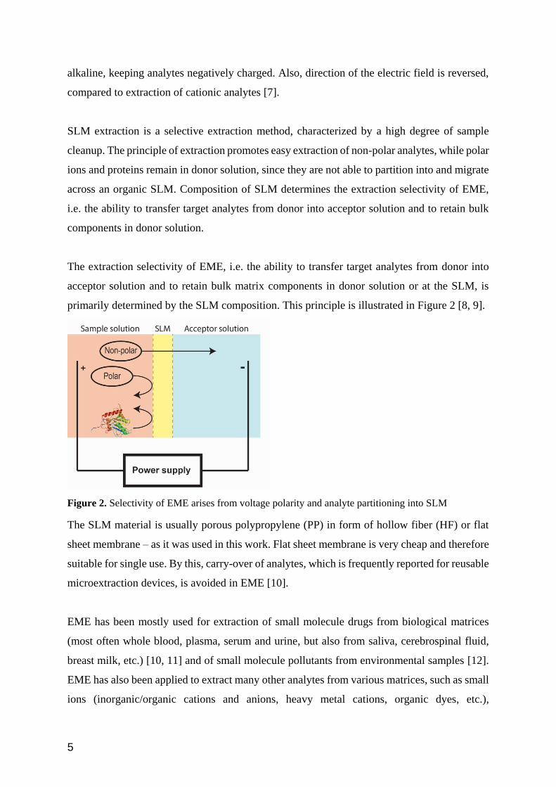
The extraction selectivity of EME, i.e. the ability to transfer target analytes from donor into
acceptor solution and to retain bulk matrix components in donor solution or at the SLM, is
primarily determined by the SLM composition. This principle is illustrated in Figure 2 [8, 9].
Figure 2. Selectivity of EME arises from voltage polarity and analyte partitioning into SLM
The SLM material is usually porous polypropylene (PP) in form of hollow fiber (HF) or flat
sheet membrane – as it was used in this work. Flat sheet membrane is very cheap and therefore
suitable for single use. By this, carry-over of analytes, which is frequently reported for reusable
microextraction devices, is avoided in EME [10].
EME has been mostly used for extraction of small molecule drugs from biological matrices
(most often whole blood, plasma, serum and urine, but also from saliva, cerebrospinal fluid,
breast milk, etc.) [10, 11] and of small molecule pollutants from environmental samples [12].
EME has also been applied to extract many other analytes from various matrices, such as small
ions (inorganic/organic cations and anions, heavy metal cations, organic dyes, etc.),

6
biochemically active compounds (amines, amino acid, peptides, hormones etc.) and different
drug metabolites [10].
Mass transfer in EME, theory
EME can be considered as a hybrid process involving both electrophoresis and distribution.
The mass transfer is principally based on electrokinetic migration, meaning that it is voltage
dependent. Efficient extraction also requires efficient distribution into the organic SLM based
on the analyte`s ability to partition into the organic phase [10].
The electrical voltage and resistance of the electrical circuit controls the amount of current in
the system. Assuming the temperature is constant, Ohms law can explain the amount of current:
I =U
R
where I is the electrical current, U is voltage and R is resistance.
In EME, the resistance of the system is mainly determined by the organic solvent used to form
the SLM, and the thickness of the membrane. To ensure adequate conductivity and penetration
of the electric field, a solvent of a certain polarity must be selected. If the conductivity becomes
too high, this can give rise to electrolysis. Considering the fact that both the artificial liquid
membrane and the model analytes are inert to electrode reactions, electrolysis will occur in the
sample and acceptor solutions, respectively[1]:
Sample solution: H2O (l) 2H+ (aq) + 1
2 O2 (g) + 2e-
Acceptor solution: 2H+ (aq) + 2e- H2 (g)
O2 and H2 are generated at the two electrodes, and the creation of bubbles increases with the
increase in current flow in the system. The pH in the sample and acceptor phase may also
change. In the acceptor phase, this can cause analytes to lose their charge, which may lead to
back-extraction, as they no longer are influenced by the electric field. To avoid pH changes,
buffer has to be used in both sample and acceptor compartments [6, 10].

7
In order to suppress bubble formation and pH changes, the electrical conductance of the
artificial liquid membrane should not be too high, but rather a compromise between the
transport efficiency and the controlled amount of electrolysis [1].
The composition of SLM is one of the crucial parameters in EME and an ideal solvent should
have the following characteristics:
1. No or very low solubility in aqueous solutions - the solvent should be immiscible with
water to avoid leakage of SLM during extraction. Therefore, solvents with water
solubility higher than 1 g/L (solubility of 1-octanol) are not recommended
2. low vapor pressure - solvent should be non-volatile to avoid evaporation of SLM during
EME
3. low viscosity - viscosity should be as low as possible to maintain high permeability
4. low but not zero conductivity - the distribution and permeation of background
electrolyte ions and sample matrix ions should be as low as possible to avoid excessive
current in the system
5. high purity - purity of SLM solvents plays important role, since solvents of lower purity
can contaminate acceptor solution during EME, therefore are solvents of higher purity
preferable [10].
One of the most used solvents in EME is 2-Nitrophenyl octyl ether (NPOE). It fulfills all the
above-mentioned criteria and was shown to be very efficient for the extraction of non-polar
basic substances (log P > 1.5) [1, 10]. However, for more polar substances (log P < 1.5), it is
necessary to add an ion-pairing reagent. Di (2-ethylhexyl) phosphate (DEHP) is typically used,
as a result, analyte partitioning now involves ionic interactions[10]. For acidic analytes,
aliphatic alcohols, such as 1-octanol have been used. However, it is reported that aliphatic
alcohols are less stable than NPOE in contact with biological fluids [6].

8
2.1.1 EME formats previously used
In order to improve enrichment, recovery and throughput, several different EME set-ups have
been developed in recent years. EME devices may be classified according to the organic layer
configuration, as illustrated in Figure 3. The first category includes devices with SLMs
consisting of polymeric membranes impregnated with organic solvent, while the second
category includes devices, which do not use any physical support for the organic layer. These
membranes are known as free liquid membranes (FLM) [10].
Figure 3. Classification of EME formats[10]
EME evolved from HF-LPME. In HF-LPME, the SLM is made of an organic phase
immobilized in the wall of a porous hollow fibre. The chemical principle is based on SLM,
however the technical set-up differs considerably. The HF-LPME system is stagnant. Set-up is
illustrated in Figure 4. The donor solution is filled into a sample vial, and acceptor solution is
placed inside the lumen of a hollow fiber impregnated with organic solvent [13, 14]. Despite
many advantages, some of the main disadvantages of using HF-LPME in bioanalysis are poor
reproducibility, due to manual cutting and sealing of the hollow fibre [15], and long extraction
time. In HF-LPME equilibrium is usually reached after 45 min [2, 14].

9
Figure 4. HF-LPME can be two phase system (A) or three phase system (B). In the two-phase system
both the SLM and acceptor compartment are filled with an organic solvent, on contrary in the three
phase system, the acceptor solution is an aqueous solution[16].
First EME set-ups used microporous HF membranes made of PP [1]. This inert hydrophobic
polymer allows impregnation with organic solvents and excellent chemical resistance against
a wide range of solvents. The acceptor container, constituted by the fiber lumen, is usually a
hollow tube with volume between 10 and 25 μL, which depends on the fiber's length and inner
diameter [17-19]. A thin platinum wire is inserted in the HF lumen and used as acceptor
electrode. Thanks to advantageous ratio of the volume of sample and acceptor compartment, a
high enrichment (up to several hundred-fold) as well as a high recovery (up to 100%) in the
traditional HF-EME configuration can be achieved in a short time [20], [21].
Parallel-EME (Pa-EME) was introduced in 2014 [22], [23]. In Pa-EME, devices with flat
membranes and multiple extractions are implemented using a 96 well-plate format. The system
consists of two well-plates, the first plate with a conductive bottom and the other one with a
polymeric membrane bottom (i.e. 96-well filter plates). Main advantages of Pa-EME compared
to previous formats are higher throughput, and use of smaller sample volumes.
Adding electrodes in both donor and acceptor solution improved reproducibility and recovery
of set-up. In this case, pH has to be adjusted so that analytes are charged in both donor and
acceptor solution. Driving force is an electric potential, thus the extraction is much faster
compared to HF-LPME [1].
Micro-EME (μ-EME) uses a sandwich approach in a horizontal configuration. Chemically inert
tube is filled successively with acceptor solution, organic layer and donor solution. Both donor

10
and acceptor solution are aqueous, and organic solution acts like free liquid membrane (FLM)
[24]. With this device, lower amount of organic phase is required. This EME format is able to
handle very low volume of samples (down to ≤ 1 μl) [25].
On-chip EME is another set-up, based on voltage-controlled extraction. Analysis can be
performed with very small sample volumes, low chemical consumption, high efficiency and
rapid extraction due to a very short diffusion path. The device consists of two poly methyl
methacrylate (PMMA) parts each with channel structure, and porous polypropylene membrane
bonded between these two substrates. The sample solution is pumped into the channel on the
sample side of the chip. From the channel, analytes are extracted through the SLM and into an
acceptor reservoir in the chip located on the other side of the SLM. The system is stagnant, and
after extraction, the acceptor solution is collected by a pipette and analyzed. A direct current
(DC) is a driving force for extraction, electrodes are placed on the bottom of the channels. On-
chip EME can be coupled directly to an analytical instrument [12].
Another format worth mentioning, which is not based on EME, but as modification of HF-
LPME is Parallel artificial liquid membrane extraction (PALME) [5]. The extraction principle
in PALME is the same as in HF-LPME. PALME consists of donor plate, acceptor plate, and a
lid. Analytes are extracted through a SLM and into an acceptor solution. Extraction occurs
during convection of the equipment on a shaker. Modification is also made on the membrane,
in PALME it is a flat membrane instead of hollow fibre, with relatively small contact area ( 0.3
cm2 ) compared to HF-LPME (1.5 cm2) [26]. In the PALME set-up the driving force is a pH
gradient. pH is adjusted so that analytes are uncharged in the sample, and charged in the
acceptor solution. [5, 27]
The device that was used in this work combines the best characteristics of different principles
– it is user-friendly with simple workflow. Consumption of organic solvent is significantly
reduced compared to traditional LLE. The characteristic that makes it unique is usage of vials
made of conducting polymers, and in theory, it could be possible to put these conducting vials
directly into the HPLC auto sampler, without having to transfer the volumes.

11
2.2 Liquid chromatography
Liquid chromatography is a method used to separate a sample into its individual components.
Separation is based on the interaction between the sample on one side, and the mobile and
stationary phases on the other side. Since many stationary / mobile phase combinations can be
used in mixture separation, different types of chromatography are classified according to the
physical states of the phases [8].
The basic physicochemical principle of chromatography is the partitioning of analytes between
two immiscible phases. The two phases move relative to each other, and in most cases, one
phase moves (the mobile phase) while the other is stationary (the stationary phase). Sample
molecules will be exposed to different interactions in the two phases simultaneously, based on
their molecule structure and nature [8].
In liquid chromatography (LC), the mobile phase is a liquid, forced through the stationary
phase of a column. Depending on the pressure of the system used, the technique is either termed
HPLC (high performance liquid chromatography) or UHPLC (ultra high performance liquid
chromatography) [28].
The main components of a chromatography system are illustrated in Figure 5.
Figure 5. Main components of LC system (retrieved from www.waters.com, February 2020)
First, the sample will mix with the mobile phase, before entering the column. This mixture will
pass through the column and further pass on to the detector and will be collected in the waste
bin. The composition of the mobile phase can be constant (isocratic elution) or varied (gradient
elution). Gradient elution is used to separate analytes with very different ability to be retained

12
on the stationary phase. The pump has a function of delivering mobile phase flow rate through
the column, thus mobile phase rate is controlled with the pump. Higher flow-rate will result in
shorter analysis time, but this also gives increased pressure in the system, and therefore requires
a lot more robust and expensive HPLC instrumentation. To ensure lower back pressure, low
viscosity mobile phase should be used, and column temperature can be increased [28].
Polarity of mobile and stationary phase determines the type of chromatography – normal phase
chromatography and reversed phase chromatography [8, 29].
In reversed phase chromatography, which is the most used separation principle in HPLC
nowadays, the mobile phase is more polar than the stationary phase. Reversed phase materials
received this name since the elution order is approximately reversed, compared to normal phase
chromatography, which was introduced first. The stationary phase comprises porous particles
(usually silica) with nonpolar groups on the surface. Most often used nonpolar groups are
different structures of hydrocarbons, with varying lengths, such as C2, C8, C18, C30, phenyl
and CN. Non-polar groups have the ability to retain the analytes by hydrophobic interaction.
Retention increases with the use of longer hydrocarbon chains, such as C18 versus C8. C18 is
the most widely used stationary phase material in reverse phase chromatography. Silica-based
stationary phases are usually stable in the range of pH 2 - 8. The mobile phase is a mixture of
an organic solvent and an aqueous phase. Important characteristic of mobile phase is elution
strength, and it is determined by the amount of organic solvent. Using a relatively higher
proportion of water than organic solvent, promotes hydrophobic interactions between the
analytes and the stationary phase. That gives better retention of analyte molecules on the
surface of the stationary phase. In contrast, an increase in the amount of organic solvent will
cause weaker interactions between the analytes and the stationary phase, hydrophobic
interactions with stationary phase will be suppressed and the affinity for the mobile phase will
be stronger. Methanol and acetonitrile are among the most commonly used organic solvents
due to their low UV cut off (190nm and 205nm respectively), relatively low cost and toxicity,
as well as their good miscibility with water. For neutral analytes, pH does not affect retention,
while it plays an important role in retention of ionic analytes [8, 29].
The columns for HPLC are commonly made from stainless steel, with the exception of
capillary and nanoflow columns that are usually made of fused silica tubing. The stationary
phase particles are held in place by frits at each end of the column. The column consists of

13
packed porous particles where pore size may vary. The standard particle size in HPLC is 5 µm
and 3 µm. The particle size have considerable importance in HPLC. A reduction in particle
size gives higher efficiency with a high number of theoretical plates, and hence narrower peaks.
This means that shorter columns can be used. Smaller particles give higher pressure. If we
decrease the size of the particles to their half, that will give four times higher pressure. At the
same time using columns with a smaller internal diameter, the peaks will be even higher and
narrower, resulting in lower mobile phase usage [8, 29].
2.2.1 UV detector
The UV detection is based on the analytes’ absorption of UV light. This requires the analyte to
contain a chromophore – functional groups that can absorb UV light. The wavelength range is
from 190 to 400 nm [8].
In the conventional UV detectors, light from a source is sent through a slit and split into
radiation of different wavelengths in a monochromator. With a filter or a grating, selected
wavelengths are passed through the sample. A signal will be obtained for all compounds that
absorb light of the appropriate wavelength.
According to Beer’s law, absorbance A is expressed by:
A = ɛ ·b·c
Where ɛ is the molar absorptivity, b is path length, and c is the concentration [29].
UV detectors can give us information about concentration of analytes, with detection limit of
0.1-1 ng [29].
2.3 Statistical method used for data analysis
Statistical design of experiments (DOE) is the process of planning and designing an experiment
in order to collect and analyze appropriate data, resulting in valid and objective conclusions
[30].

14
In DOE, factors are defined as the variables, that are controlled during an experiment by the
ones performing experiment (independent variables) in order to determine their effect on the
response variable. Response variables are also known as dependent variables, y-variables, and
outcome variables. The settings of a factor is usually referred to as the factor level. A typical
aim of DOE is to determine whether changes in the independent variables correlates with the
changes in the response. [31]
The one-factor-at-a-time method (OFAT) is a very common experimental technique and
consists of choosing the starting point for each factor and then varying each factor over its
range while having all the other factors constant. Varying one at a time instead of multiple
factors simultaneously. A major limitation of the OFAT approach is that the study of all factors
possibly involves huge number of tests, and it excludes potential interaction between the
factors. Interaction between factors often occur, and failing to account for these in decision-
making may result in poor/unexpected outcomes [30].
The factor effect is defined as the response change created by a change in the factor level. This
is called main effect. In some experiments, we may notice that the difference in response
between the levels of one factor is not the same at all levels of the other factors, this is called
interaction between the factors [30].
An often more suitable strategy for dealing with multiple factors is performing a factorial
experiment, which means that variables are varied together rather than one at a time. Generally,
if there is k number of factors, the factorial design would require 2k runs, assuming that each
factor has 2 levels. This is called a full factorial design. However, the number of experiments
will also be high, as long as we have many factors. Fortunately, it is usually not necessary to
run all possible combinations of factor levels. A fractional factorial experiment is a
modification of the basic design, in which only a small number of rounds are used [30].
There are several main advantages of factorial experiments over one-factor-at-a-time (OFAT):
- OFAT cannot predict interactions
- Factorial designs are more efficient than OFAT experiments – in terms of cost and time.
More information is provided at similar or lower cost. Optimal conditions can be found
faster than OFAT studies.
- With factorial design it is possible to investigate additional factors at no additional cost

15
- Factorial designs enable estimation of the effects of one factor to various levels of the
other factor, resulting in conclusions applicable over a range of experimental conditions
[32].
The simplest design in the 2k series is one with lowest number of factors and levels. For
instance, two factors, say A and B, each run at two levels. This design is called a 2-2 factorial
design. The levels of the factors may be called “low” and “high.” These two levels may be
quantitative, or they may be qualitative. In most studies the factors and their levels are
quantitative.
All of the factors and levels perform factorial experiments. For example, in a 2 x 2 (“two-by-
two) factorial design, we have two factors with two levels for each factor. A 2k full factorial
design has k factors, each with 2 levels, and n = 2k runs consisting of all level combinations of
the k factors.
After obtaining results, the factorial experiment can be analyzed using analysis of variance
(ANOVA) or regression analysis. ANOVA tests the hypothesis that the mean values of two or
more populations are equal. Through comparing the response variable means at the various
factor levels, ANOVA determines the importance of one or several factors. The null hypothesis
assumes that all population means (factor level means) are equal, while the alternative
hypothesis says that at least one is different.
ANOVA requires continuous response variable and at least one independent factor with two or
more levels. It is also necessary that data originate from approximately normally distributed
populations with equal variances between factor levels. However, even when the normality
principle has been compromised, ANOVA procedures are working quite well, except when
one or more distributions are highly distorted or if the variances are quite large. This can be
fixed with transformation of the original dataset.
The p-value is the probability of achieving the observed test results, given the null hypothesis
is correct. A lower p-value means that the alternative hypothesis provides stronger evidence.
P-values are calculated using p-value tables or spreadsheets/statistical software [30].
16
As mentioned above – as the number of factors in 2k factorial design increases, so does the
number of runs, often exceeding available time and resources. Assuming that some of high-
order interactions (interactions of 2 or more factors) are insignificant, it is possible to obtain
information regarding main effects and low-order interactions only by using a fraction of the
entire factorial experiment, i.e. fractional factorial designs. They are among the most
commonly used types of designs for product development and process design, process
improvement and industrial/business experimentation [30].
In practical work, it means that we only perform for example ½ or ¼ of the experiment runs,
for ½ and ¼ fraction respectively. Even though we are decreasing the number of runs, data
obtained are significant because we give up estimation of some high-order interaction terms
[31].
For example, if we have a 26 factorial design – meaning that we have 6 factors with two levels
for each factor, total number of runs would be 64 in a full factorial design. In fractional
factorials, we can give up 6-factors interaction ABCDEF (high-order interaction), assuming
that A = A + ABCDEF. So, we estimate these two factors combined, this is called aliasing.
However, if interaction ABCDEF does not exist then we are estimating only A. When we do
these designs, it is determined which factors are aliased. In general, we try to have main effects
(1 letter factor – A or B) aliased with the highest possible interaction order (ABCDEF for 6-
factor design).
The presumption of linearity in the factor effects is a potential concern for the two-level
factorial design. Perfect linearity is unnecessary, and the 2k system will work well even when
the linearity assumption holds only approximately. A solution to detect deviation from linearity
is addition of center points.
Center points are added to experimental setting runs for two purposes:
- To provide a measure of process stability or if our model is reliable – center points are
spread evenly through the list of experiments, so that we can monitor process stability
- They are useful for finding and estimating curvature.
For quantitative factors, center points have value in the middle of the level scale. If the low
value is 1, and the high level is 3, then the center point is 2. [30]
17
More complex design than simple 2-level factorial is a response surface model (RSM). It is a
collection of mathematical and statistical techniques useful for the modeling and analysis of
problems in which a response of interest is influenced by several variables and the objective is
to optimize the response [30]. For this, we use both factorial points (-1 and +1), center points
(denoted “0”) and “star” points. Star points (= axial points) are outside the factorial points. This
can be at “-2” or “+2”. Level of the star point will vary from the number of factors and from
what is practical. One factor’s star points are found outside the factorial points for that factor,
while all other factor are set to their center point value. Star points help estimating curvature
and (like center points) provide more data to make model more valid.
A regular 2-level factorial can also tell us if a factor has effect on the response, and if the effect
is positive or negative. It is not good for predicting the exact magnitude of the effect. An RSM
model can do this.
An RSM model can also allow us to find the optimum factor settings, and it can describe how
the system behaves over the whole range of all factors, not just the optimum. With the RSM
model, we can thus predict how the transition from one factor setting to another, will have an
effect on the response. [31].

18
3 Experimental
3.1 Model analytes
Model analytes, in this work, were prepared in stock as 1 mg/ml solution of five drugs –
pethidine, nortriptyline, methadone, haloperidol and loperamide, in ethanol. For extractions,
stock solution was diluted to 5 μg/ml in 10 mM HCl. All five drugs are basic lipophilic
molecules (Table 1).
Table 1. Molecular structure (downloaded from www.chemspider.com), pKa and log P (retrieved
from www.chemicalize.com ) of model analytes
Analyte Structure pKa Log P
Pethidine
8.16 2.14
Haloperidol
8.05 3.66
Nortryptilin
10.47 4.43
Methadone
9.12 5.01
Loperamide
9.41 4.77

19
3.2 Chemicals
All chemicals used in this work are listed in Table 2.
Table 2. List of chemicals with purity grade and producer
Chemical Purity Producer
Water Ion-exchange, Milli Q Millipore (Oslo, Norway)
Acetonitrile (C2H3N) 99.9% Merck KGaA (Darmstadt,
Germany)
Formic acid (HCOOH) 98% Fluka Chemie GmbH (Buchs,
Switzerland)
2-Nitrophenyloctyleter
(O2NC6H4O(CH2)7CH3)
≥ 99 % Sigma-Aldrich GmbH
(Steinhem, Germany)
Hydrochloric acid (HCl) 37% Merck KGaA (Darmstadt,
Germany)
Ethanol (C2H5OH) 96% Arcus (Nittedal, Norway)
3.3 Solutions
Stock solutions
For the experiments, stock solutions of the model analytes were made and used for further
experiments.
1 mg/ml 5 bases
5 bases: 20 mg of pethidine, haloperidol, nortriptyline, methadone and loperamide,
respectively, were weighed and dissolved in 20 ml of ethanol, to a final concentration of
1 mg/ml.
Standard solution
The standard solutions of 5 µg/ml concentration were prepared by pipetting out 50 µl stock
solution in 10 a ml volumetric flask and further diluted with 10 mM HCl to 10 ml. All the
solutions were stored in refrigerator when not in use.
10 mM HCl
83 μl of 37 % hydrochloric acid was dissolved up to 100 ml of deionized water

20
3.4 EME set-up
The equipment used for EME was obtained from G&T Septech AS, Ski, Norway and is
illustrated in Figure 6.
Union
Figure 6. EME set-up. Electro-conducting vials separated with union. SLM membrane is placed
inside the union.
The EME set up consisted of two vials, made of conducting materials. Vials are separated with
a non-conducting plastic SLM membrane holder, called the union. This union can be either
with or without lip. In the case when the union without lip was used, two teflon rings were put
on both sides of the polypropylene membrane, while union with lip demands addition of just
one teflon ring. The SLM supporting membrane is polypropylene membrane and it was made
using a 9 mm hole pipe, i.e. membrane diameter was 9 mm. Unlike traditional EME, with
platinum electrodes inserted in the sample and acceptor solution, ring electrodes placed around
conducting vials were used for electric contact.
The EME set was placed on a mechanical laboratory agitator. The electrodes were coupled to
a DC power supply (model ES 0300-0,45, Delta Elektronika V.B, Zierikzee, Netherland). A
Fluke 287 multimeter (Everett, Washington, USA) at an acquisition rate of 8 Hz, was
connected with the power supply in order to monitor current (Figure 7).
Figure 7. EME set-up placed on mechanical laboratory agitator, connected to DC power supply (left),
conducting vials with ring electrodes (right)
Vials made of electro-
conducting materials

21
3.4.1 Procedure for EME
Primarily, the polypropylene membrane was placed inside the union. In the majority of
experiments, a union with lip was used, meaning that one teflon ring was added. Secondly,
acceptor solution (10mM HCl), was added in acceptor vial, followed by assembling acceptor
vial to the treaded top part (union + membrane + teflon ring). After this step, NPOE was
pipetted to the membrane from the donor/sample side. The donor solution was pipetted to the
donor vial and assembled to the second treaded top part (Figure 8) The ring electrodes were
put on the vials. The assembly was placed on a mechanical laboratory agitator. Finally, the
electrical field was coupled by connecting ring electrodes to the power supply, paying attention
that donor/sample vial has to have positive potential and acceptor vial negative potential. After
extraction, 100 μl of solution from acceptor vial was pipetted into vials with inserts for HPLC-
UV analysis.
Figure 8. Procedure for EME – simplified schematic figure of first steps in EME

22
In all the experiments, different parameters – including extraction time, volume of sample
and acceptor solution, volume of NPOE, voltage and shaking rate were used.
3.5 HPLC-UV
After EME, separation of model analytes was performed using an Agilent 1200 Series HPLC
(Agilent Technologies, Santa Clara, CA, USA). The column was Gemini C18 reverse-phase
column (Phenomex, Torrance, CA, USA), length was 150 mm, particle size was 5 µm and
inner diameter was 2.0 mm. For the detection, a UV-DAD detector with Agilent ChemStation
for LC 3D Systems as software was used. Model analytes were separated using HPLC
parameters described in Table 3, and gradient elution as shown in Table 4.
Table 3. HPLC parameters
Parameter Value
Flow rate 0.400 ml/min
Mobile phase A 95:5 20 mM Formic acid:ACN
Mobile phase B 95:5 ACN:20 mM Formic acid
Run time 25 min
Column temperature 60 oC
Mobile phase A was prepared by dissolving 50 ml of ACN in 950 ml 20 mM formic acid, and
mobile phase B was made dissolving 50 ml of 20 mM formic acid solution in 950 ml ACN.
Table 4. HPLC gradient

23
Time
(min)
Mobil phase A Mobil phase B
0 100% 0%
15.00 60% 40%
17.00 60% 40%
17.10 0% 100%
21.00 0% 100%
21.10 100% 0%
25.00 100% 0%
UV-detection was performed at 235 nm.
3.6 Calculations
The concentration of each analyte in the acceptor solution after EME was calculated using the
formula:
𝐶𝑎 =𝑊𝑝
𝑊𝑠𝑡𝑑∙ 𝐶𝑠𝑡𝑑
where Ca is the concentration of analyte in the acceptor solution, Wp is the peak area of the
analyte from the acceptor phase, Wstd is the peak area for the analyte from the standard solution,
and Cstd is concentration of the standard solution.
The recovery of each analyte after extraction was calculated by formula:
𝑅 =𝑛𝑎
𝑛𝑝∙ 100% =
𝑉𝑎 ∙ 𝐶𝑎
𝑉𝑝 ∙ 𝐶𝑝∙ 100%
where R is the recovery of analyte in %, na is the number of moles of analyte in the acceptor
phase after extraction, while np is the number of moles of analyte in the sample before the
extraction. Va and Vp are volumes of respectively the acceptor solution and sample, Ca and Cp

24
are the concentration of analyte in the acceptor solution after extraction, and in the sample
before extraction.
3.7 Data analysis
The designed experiments were generated and analyzed using Design-Expert V12 trial version
(Stat-Ease Inc., MN, USA).

25
4 Results and discussion
The overall aim of the study was optimization of the new prototype design. The term
optimization has been commonly used in analytical chemistry as a means of discovering
conditions at which to apply a procedure that produces the best possible response [33].
All experiments belonged to the following categories:
- Stage 0: experiments where the main goal was to get initial experience with the
device and with operational conditions. Stage 0 included all results before the
designed experiments.
- Stage 1: Screening of parameter and factor settings
- Stage 2: Search of optimal region by method of steepest ascent
- Stage 3: Full optimization with response surface modeling
4.1 Initial experience with the device
In the initial tests of the prototype device, a different configuration than what is described in
Section 3, was used. Instead of ring electrodes around the conducting vials, a compartment box
holder was used to provide the electric contact (Figure 9). This was part of the original
prototype device supplied by the manufacturing company. The set up consisted of two vials
connected via a union, and this set-up was put in the holder compartment connected to
electrodes via crocodile clips (Figure 10). Here, electrodes were connected to the vials in just
one point (Figure 11).
Figure 9. Compartment box units

26
Figure 10. Vials of conducting polymer inside compartment box
Figure 11. Connecting point between vial and compartment box
With this set-up, several parameters related to the extraction were investigated, in order to
obtain high recovery with acceptable standard deviation. Extraction time was varied from 5 to
45 minutes. Volume of both sample and acceptor solution were considered as important factors
since these might affect both extraction kinetics and repeatability. These were thus varied from
500 μl to 1500 μl of both sample/acceptor. The maximum volume each vial could hold was
approximately 1800 μl, and this was therefore the limiting factor. With these parameters
established the volume of SLM, agitation rate and voltage were found to have no or very little
impact on the results.
Connecting point

27
However, several challenges with this prototype device were identified during
experimentation. The first problem that occurred was unstable current during each extraction.
Current fluctuated during each extraction, as well as between succeeding extractions. This was
attributed to inadequate contact between vials and electrodes connected via holder box. The
poor electrical contact resulted in lower extraction recoveries, and higher relative standard
deviation. The best results were obtained using 1500 μl of both donor and acceptor solution,
extraction time was 30 min, voltage was 100 V, volume of NPOE (SLM) was 11μl, and an
agitation rate of 1050 rounds per minute (rpm). The extraction recoveries are shown in Figure
12. As seen, the recovery ranged from 20% to 70% for the five model analytes, with relative
standard deviation (RSD) of about 20%. Increasing the extraction time to 45 minutes did not
improve the extraction efficiency, indicating the system had reached a steady-state after 30
minutes.
Figure 12. Recovery of model analytes after three subsequent extraction under same conditions –
1500 μl of donor and acceptor solution, 30 min extraction time, voltage 100 V, agitation was 1050
rpm and 11μl of SLM, using holder box as connection point between the vials and electrodes
Figure 13. Relative standard deviation (RSD %) of area under curve after three subsequent
extractions under same condition (see Figure 12)
70%63%
68%
51%
23%
41% 41% 40%45%
13%
58%
35% 35%40%
23%
0%
10%
20%
30%
40%
50%
60%
70%
80%
Petidin Haloperidol Nortryptilin Metadon Loperamid
Recovery %
EME 1 EME 2 EME 3
0 5 10 15 20 25 30
Petidin
Haloperidol
Nortryptilin
Metadon
Loperamid
RSD %

28
As seen from the graphs, the extraction recoveries obtained in the best case were only up to
70%, and the relative standard deviation was somewhat higher than what has previously been
reported for these compounds [1, 4, 5, 34]. The poor extraction performance and unstable
current lead us to the conclusion that the main issue with set-up was inhomogeneous
conductivity of the vials. Upon further investigation, the problem was located at the connecting
point between the vials and the holder box. Because this connecting point provided poor
electric contact, the system was vulnerable to variation between extractions, and the actual
electric field that drives the extraction was too low to give high extraction efficiency.
After identifying the problem, changes in the set-up were considered necessary in order to get
stabile current during extraction. One of the solutions tested was to put ring electrodes around
the conducting vials. By this, better contact between electrodes and the vials was achieved.
This produced a stable current during repeated extraction. All further experiments were thus
performed on the new set-up, consisting of ring electrodes around conducting vials.
4.2 Stage 0 - Preliminary testing
The overall aim was to characterize the commercial device and to identify the optimal
operational parameters. Five main independent variables were expected to have a major effect
on the recovery. These factors were:
1. Volume of donor and acceptor solution
2. Voltage
3. Volume of SLM
4. Shaking speed
5. Shaking time
For performing further experiments, the following standard conditions were used (Table 5).
In the next step, stage 0, the aim was to find a general frame of parameters that affected the
device’s performance – i.e. which factor levels could be used, how high recovery could be
obtained, and the variability of recovery for these settings. The extraction performance was
considered satisfactory for %RSD < 20, which was required before subsequent designed
experiments could be performed.

29
Table 5. Standard conditions for optimization of the device
Membrane Polypropylene PP2E
Sample/Donor 1500 μl 5 μg/ml model analytes in 10 mM HCl
SLM 11 μl NPOE
Agitation 1050 rpm
Time 15 min
Voltage 100 V
Replicates x 3
Analysis HPLC-UV
Several experiments with variation of standard conditions were conducted, in order to get a
general understanding of the system. Volumes of sample and acceptor solution were the same.
In all the experiments, NPOE was used as SLM. In this stage of analysis, both union with or
without lip was used. The extraction results obtained by varying different parameters are shown
in Table 6.

30
Table 6. Recovery and %RSD of preliminary testing with two replicates for each set of conditions
Pethidine Haloperidol Nortriptyline Methadone Loperamid
700μl donor and acceptor, 11μl
NPOE, 1400 rpm, 15min, 100V,
with lip
Recovery 75 % 78 % 83 % 89 % 79 %
RSD% 15 % 5 % 6 % 10 % 9 %
700 μl donor and acceptor, 11μl
NPOE, 1400 rpm, 10 min, 100V
with lip
Recovery 52 % 64 % 63 % 52 % 71 %
RSD% 15 % 8 % 8 % 10 % 6 %
1500 μl donor and acceptor, 11μl
NPOE, 15min, 1400 rpm, 50V,
without lip
Recovery 44 % 43 % 46 % 42 % 49 %
RSD% 20 % 17 % 13 % 8 % 21 %
1500 μl donor and acceptor, 11μl
NPOE, 15min, 1400 rpm, 50V with
lip
Recovery 53 % 44 % 50 % 36 % 41 %
RSD% 35 % 7 % 5 % 21 % 22 %
1500μl donor and acceptor, 11μl
NPOE, 1400 rpm 15 min, 100V,
without lip
Recovery 45 % 47 % 51 % 54 % 41 %
RSD% 12 % 12 % 12 % 10 % 3 %
1500μl donor and acceptor, 11μl
NPOE, 15 min, 1400 rpm, 100V
with lip
Recovery 44 % 42 % 48 % 62 % 38 %
RSD% 8 % 4 % 5 % 2 % 4 %
1000 μl donor and acceptor, 11μl
NPOE, 15 min, 1400 rpm, 100V
with lip
Recovery 52 % 52 % 56 % 57 % 45 %
RSD% 8 % 7 % 7 % 10 % 8 %
1500 μl donor and acceptor, 9μl
NPOE, 15min, 1400 rpm, 100V
with lip
Recovery 47 % 46 % 49 % 50 % 43 %
RSD% 8 % 6 % 6 % 10 % 9 %
1500 μl donor and acceptor, 12 μl
NPOE, 1400 rpm, 15 min, 100 V,
with lip
Recovery 41 % 41 % 46 % 38 % 35 %
RSD% 5 % 4 % 9 % 8 % 5 %
As shown in Table 6, higher recoveries were achieved with lower volume of both sample and
acceptor solution – an average recovery higher than 75% was, as such obtained using 700 μl
of sample and acceptor solution. On the other side, increasing volume of sample and acceptor
solution to 1500 μl, gave recovery of around 50%. RSD values were generally lower than 20%
and the system was therefore considered stable enough to proceed with designed experiments.
31
4.3 Stage 1 - Screening of parameter and factor
settings
Results after preliminary testing were used as starting point for further optimization. For
screening and optimization of factors relevant to the extraction, a design-of-experiments
methodology based on factorial designs was used.
In stage 1, a screening design augmented with center points was used. A screening design such
as this is able to identify if factors are significant and if they affect the response positively or
negatively. The use of center points additionally allowed detecting curvature in the system,
indicating that one or multiple factors had an optimal setting within the tested factor range,
however, the screening design contained too few experimental points to estimate which factors
had an optimum. The purpose was thus to evaluate the relative importance of the factors
included.
The average recovery of the five model analytes was used as the response variable, and the
results were analyzed with ANOVA. Practically, the factor settings for the five parameters
(extraction time, volumes of donor/acceptor solution, voltage, shaking and SLM volume) was
determined ‘’low’’, ‘’high’’ and center point (mean of both ‘’low’’ and ‘’high’’ value). The
design included 20 runs, divided into two blocks. The point with division into the blocks was
to exclude parameters that could have effect on our response variable, without having
possibility to control them, such as running the experiments during two days. By dividing
experimental runs into homogeneous blocks, the sensitivity of DOE increases. A detailed
description of experiment and results are illustrated in Table I (Appendix).
The primary aim was to determine whether these five parameters have effect and whether it is
positive or negative effect on recovery. The ANOVA data after the statistical analysis are
shown in Table 7.

32
Table 7. ANOVA table for factors found to be significant
Source Sum of Squares Df Mean Square F-value p-value
Model 12401.0 13 953.9 32.4 < 0.0001 Significant
Blocks 6.2 1 6.25 0.21 0.661 not significant
A-Time 4425.2 1 4425.2 150.1 < 0.0001
B-Voltage 688.3 1 688.3 23.3 0.0013
C-Shaking 1848.0 1 1848.0 62.7 < 0.0001
D-Volumes 1863.3 1 1863.3 63.2 < 0.0001
E-SLM volume 417.1 1 417.1 14.2 0.009
AC 192.7 1 192.7 6.5 0.043
AD 524.3 1 524.3 17.8 0.006
AE 240.6 1 240.6 8.2 0.029
BD 337.8 1 337.8 11.5 0.015
CD 645.0 1 645.0 21.9 0.003
DE 402.0 1 402.0 13.3 0.010
Curvature 810.6 1 810.6 27.5 0.002
Residuals 176.9 6 29.5
Lack of Fit 130.3 4 32.6 1.4 0.458 not significant
Pure Error 46.6 2 23.3
Cor Total 12577.9 19
Based on average recovery as response variable, data analysis showed which main effects and
interactions were significant. The Model F-value of 40.24 implies the model is significant.
There is only a 0.01% chance that an F-value this large could occur due to noise.
P-values less than 0.05 indicated that model terms were significant. In this case A, B, C, D, E,
AC, AD, AE, BD, CD, DE were significant model terms. Values greater than 0.05 indicated
the model terms were not significant and these were thus excluded from the model. As seen,
the block was found not significant and the results were therefore not affected by running the
experiments over two days.

33
A model can be considered well fitted to the experimental data if it presents a significant
regression and a non-significant lack of fit. In other words, the major part of variation
observation must be described by the equation of regression, and the remainder of the variation
will be due to the residuals. Most variation related to residuals is due to pure error (random
fluctuation of measurements) and not to the lack of fit, which is directly related to the model
quality. In our example, the lack of fit F-value of 1.4 implies the Lack of Fit is not significant
relative to the pure error. There is a 45.8% chance that a Lack of Fit F-value this large could
occur due to noise. This means that as long as we get non-significant lack of fit – one of the
conditions that the model fits is fulfilled.
Two-level factorial designs assume there is a linear relationship between each X and Y.
Therefore, if the relationship between any X and Y exhibits curvature, a two-level factorial
design should not be used because the results may be misleading. However, by using center
points we can statistically determine if the relationship is linear or nor. If the curvature p-value
is significant, we can conclude that curvature exists. In this case, the experimental design can
be expanded to perform response surface modeling—such as with a central composite design,
which can enable estimation of curvature of individual factors. Classical two-level factorial
designs can thus detect curvature, while response surface designs can model (build an equation
for) the curvature.
Examining residuals is a key part of all statistical modeling, including DOE's. Looking at
residuals can tell us whether our assumptions are reasonable and our choice of model is
appropriate. Residuals can be thought of as elements of variation unexplained by the fitted
model. Since this is a form of error, the same general assumptions apply to the group of
residuals that we typically use for errors in general: one expects them to be (roughly) normal
and (approximately) independently distributed with a mean of 0 and constant variance.
The normal probability plot indicates whether the residuals follow a normal distribution, in
which case the points will follow a straight line (Figure 14). The visual inspection of the
residual graphs can also generate valuable information about the model suitability. Thus, if the
mathematical model is well fitted, its graph of residuals presents behavior that suggests a
normal distribution. The normal probability plot should produce an approximately straight line

34
if the points come from a normal distribution. Underlying assumption of normally distributed
residuals is met in our data.
Figure 14. Normal Plot of Residuals – approximately straight line means that residuals follow normal
distribution
Another valuable set of information gained from this stage of experiments is effects graphs for
all five factors. They are used in order to visualize the magnitude, direction, and the importance
of the effects. Figure 15 shows the effect plots of the five factors included in the model. All
factors, except for volume of donor/acceptor, had a positive effect on the extraction recovery.
While there were many significant two-factor interactions, these only affected the magnitude
of the difference from low to high factor setting, not the direction of the effect. With visual
inspection we can see that the center points are higher than the linear lines from low to high,
showing curvature in the system.

35
Figure 15. Model graphs for all factors presented as response to recovery
4.4 Stage 2 - Search of optimal region by method of
steepest ascent
In the next step, stage 2 or Path of steepest ascent, data gained through previous set of
experiments, showed in which direction parameters should be adjusted in order to get the best
possible recovery. Region of optimal parameter settings could potentially be found outside the
factor ranges of the screening design. Once this region was located, the final optimization could
be performed.
The method of steepest ascent provides experimental moves in a specific direction to explore
a new area of potentially improved method performance.[35]
Stage 2 set of experiments were performed according to parameters illustrated in Table 8, 2
replicates of each, following the path of steepest ascent for each factor. The first experiment
level was equal to the center points of the screening design.
36
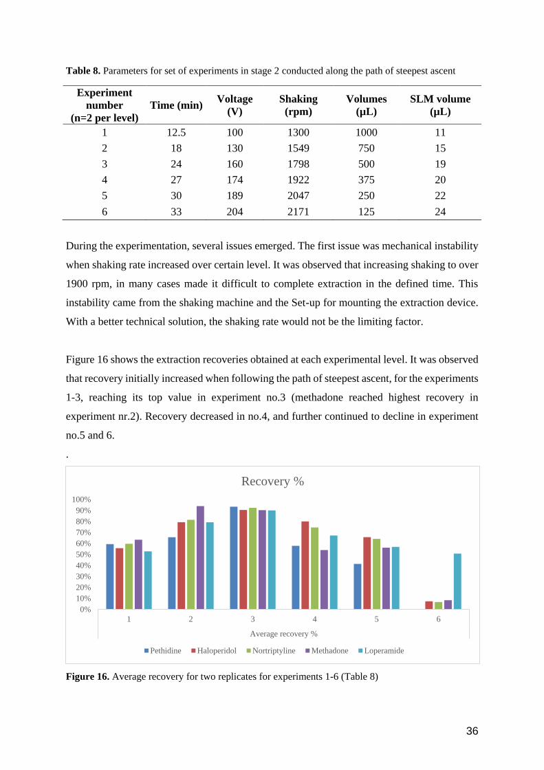
Table 8. Parameters for set of experiments in stage 2 conducted along the path of steepest ascent
Experiment
number
(n=2 per level)
Time (min) Voltage
(V)
Shaking
(rpm)
Volumes
(µL)
SLM volume
(µL)
1 12.5 100 1300 1000 11
2 18 130 1549 750 15
3 24 160 1798 500 19
4 27 174 1922 375 20
5 30 189 2047 250 22
6 33 204 2171 125 24
During the experimentation, several issues emerged. The first issue was mechanical instability
when shaking rate increased over certain level. It was observed that increasing shaking to over
1900 rpm, in many cases made it difficult to complete extraction in the defined time. This
instability came from the shaking machine and the Set-up for mounting the extraction device.
With a better technical solution, the shaking rate would not be the limiting factor.
Figure 16 shows the extraction recoveries obtained at each experimental level. It was observed
that recovery initially increased when following the path of steepest ascent, for the experiments
1-3, reaching its top value in experiment no.3 (methadone reached highest recovery in
experiment nr.2). Recovery decreased in no.4, and further continued to decline in experiment
no.5 and 6.
.
Figure 16. Average recovery for two replicates for experiments 1-6 (Table 8)
0%
10%
20%
30%
40%
50%
60%
70%
80%
90%
100%
1 2 3 4 5 6
Average recovery %
Recovery %
Pethidine Haloperidol Nortriptyline Methadone Loperamide

37
It is worth mentioning that under ideal circumstances, an additional screening experiment with
factor levels set around experiment no.3, would be performed to evaluate if all factors had in
fact an optimum near this level. However, due to time constraints this was not performed.
4.5 Stage 3 - Response surface model optimization
The factor settings, identified as approximately optimal in stage 2, were then used as the
starting point for stage 3, the final optimization by response surface modeling (RSM).
Determining the response surface for each factor has the additional advantage, besides enabling
optimization, that the behavior of the device may be better understood. Additionally, if one or
more factors are constrained (e.g. short extraction time) the response surfaces allow
identification of changes to other factors that provide new optimal conditions.
For optimization of extraction conditions, a five factor central composite design (CCD) that
included factorial-, center-, and star-points was chosen.
The central composite design consists of the following parts:
(1) A full factorial or fractional factorial design;
(2) An additional design, often a star design in which experimental points are at a distance from
its center. This distance, termed 𝛼, is ideally the square root of the number of factors. However,
if this results in extreme factor setting outside what is practically possible, a “practical” 𝛼 value
of 1.5 may be used
(3) center points [33].
In our model following points were used (Figure 17)
Factorial: High/low factor level (+1/-1),
Center points: Estimate variance, curved response, check stability
Star points: Help estimate curvature but are not part of prediction range. The coded
factor levels for the star points were set as±1.5.

38
Figure 17. Factorial points, center and star points
To minimize the required number of experiments the factorial points were run as ½ fractional
factorial, giving a total of 32 runs. All factors were studied in five levels. The average extraction
recovery of the replicates was used as response factor. Response variable was average recovery
for all molecule analytes.
After set of experiments performed according to parameters shown in Table II in Appendix,
the results gained were analyzed with ANOVA (Table 9).
Factorial points
Center points
Star points
39
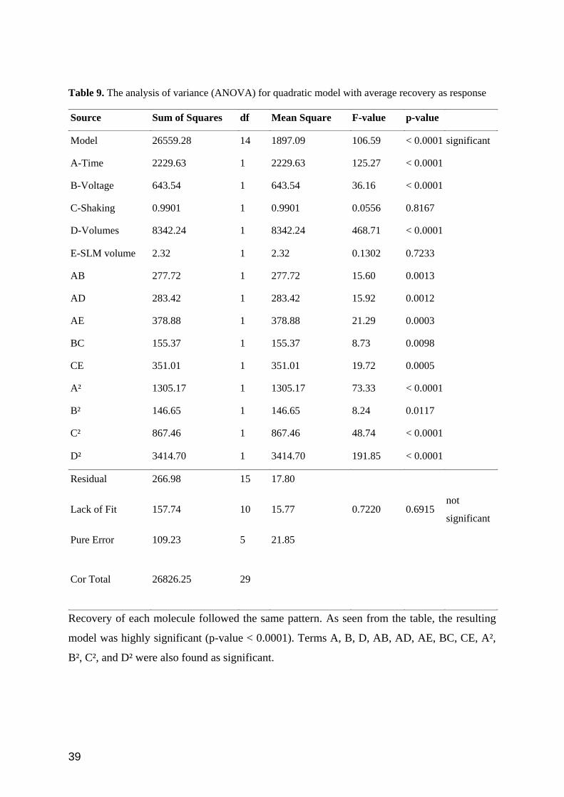
Table 9. The analysis of variance (ANOVA) for quadratic model with average recovery as response
Source Sum of Squares df Mean Square F-value p-value
Model 26559.28 14 1897.09 106.59 < 0.0001 significant
A-Time 2229.63 1 2229.63 125.27 < 0.0001
B-Voltage 643.54 1 643.54 36.16 < 0.0001
C-Shaking 0.9901 1 0.9901 0.0556 0.8167
D-Volumes 8342.24 1 8342.24 468.71 < 0.0001
E-SLM volume 2.32 1 2.32 0.1302 0.7233
AB 277.72 1 277.72 15.60 0.0013
AD 283.42 1 283.42 15.92 0.0012
AE 378.88 1 378.88 21.29 0.0003
BC 155.37 1 155.37 8.73 0.0098
CE 351.01 1 351.01 19.72 0.0005
A² 1305.17 1 1305.17 73.33 < 0.0001
B² 146.65 1 146.65 8.24 0.0117
C² 867.46 1 867.46 48.74 < 0.0001
D² 3414.70 1 3414.70 191.85 < 0.0001
Residual 266.98 15 17.80
Lack of Fit 157.74 10 15.77 0.7220 0.6915 not
significant
Pure Error 109.23 5 21.85
Cor Total 26826.25 29
Recovery of each molecule followed the same pattern. As seen from the table, the resulting
model was highly significant (p-value < 0.0001). Terms A, B, D, AB, AD, AE, BC, CE, A²,
B², C², and D² were also found as significant.
40
As can be seen from Table 9, main effect of shaking and SLM volume were not significant,
considering the fact that their p-value is greater than 0.05. Both factors are however involved
in significant interactions, and can therefore not be excluded from the model.
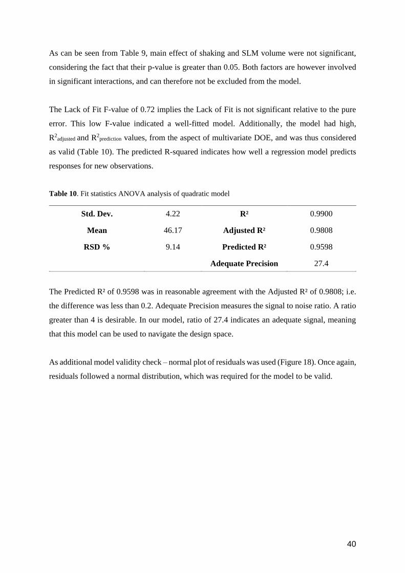
The Lack of Fit F-value of 0.72 implies the Lack of Fit is not significant relative to the pure
error. This low F-value indicated a well-fitted model. Additionally, the model had high,
R2adjusted and R2
prediction values, from the aspect of multivariate DOE, and was thus considered
as valid (Table 10). The predicted R-squared indicates how well a regression model predicts
responses for new observations.
Table 10. Fit statistics ANOVA analysis of quadratic model
Std. Dev. 4.22 R² 0.9900
Mean 46.17 Adjusted R² 0.9808
RSD % 9.14 Predicted R² 0.9598
Adequate Precision 27.4
The Predicted R² of 0.9598 was in reasonable agreement with the Adjusted R² of 0.9808; i.e.
the difference was less than 0.2. Adequate Precision measures the signal to noise ratio. A ratio
greater than 4 is desirable. In our model, ratio of 27.4 indicates an adequate signal, meaning
that this model can be used to navigate the design space.
As additional model validity check – normal plot of residuals was used (Figure 18). Once again,
residuals followed a normal distribution, which was required for the model to be valid.

41
Figure 18. Normal plot of residuals model fitted to average extraction recovery
To further visualize the model fit, a plot of predicted vs actual values was made (Figure 19).
Even distribution of points around the diagonal indicates better correlation between predicted
and observed responses. This further elucidates the aptness of the model for optimization.
Figure 19. Comparison between the actual values and the predicted values of RSM model. Two
cross-out points were considered outliers and therefore not included in the data interpretation

42
RSM experiments result in a model that describes a response as a function of the varied factors
and levels. The figures below show surface plots with different parameters and main effects.
Figure 20 shows the surface of time and voltage. As seen, some improvement at higher voltage
could be achieved. However, increasing time yielded higher recovery until a certain level
where a minor decrease was observed. To verify the importance of voltage, a few extractions
were performed at 0 V (data not shown). Here, no extraction occurred. When voltage was
increased from 0 to 80 V, recoveries however increased significantly. This trend is consistent
with many previous reports on EME [1].
Figure 20. Response surface plot in 3D, average recovery in % as function of time and voltage
Figure 21 shows the surface plot of volumes and shaking rate. Viewing these factors together
is relevant, as the optimal settings may be dependent upon each other. As seen, the settings that
resulted in the highest average recovery was approximately 850 µl and 1400 rpm. However,
previous experiments (Figure 16) indicated 500 µl at high shaking rate is also efficient. In the
present sequence of experiments, the lowest level of sample/acceptor volume was set to 250
µl. However, this was too low as most experiments with this volume resulted in approximately
0 % recovery (Table II). This is expected to have affected the estimated model for lower
volumes.
43
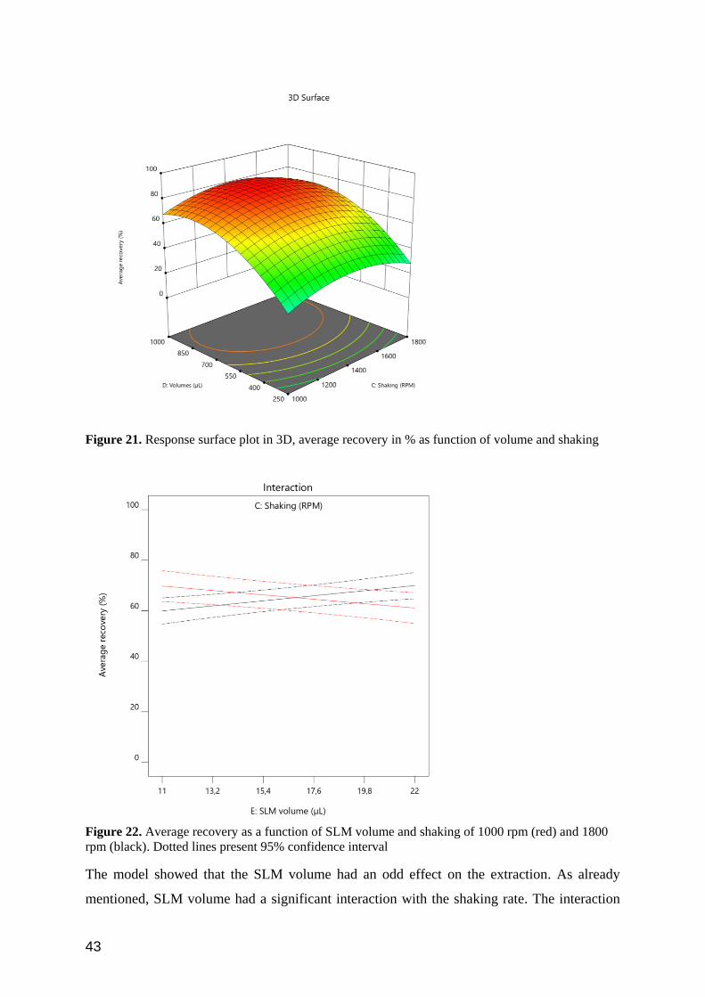
Figure 21. Response surface plot in 3D, average recovery in % as function of volume and shaking
Figure 22. Average recovery as a function of SLM volume and shaking of 1000 rpm (red) and 1800
rpm (black). Dotted lines present 95% confidence interval
The model showed that the SLM volume had an odd effect on the extraction. As already
mentioned, SLM volume had a significant interaction with the shaking rate. The interaction

44
meant that the recovery will be higher if we use lower volume of SLM at 1800 rpm. However,
decreasing the shaking rate to 1000 rpm would require higher volume of SLM in order to get
recovery over 60% (Figure 22). One of possible explanation for this occurrences is that excess
of NPOE is maybe shaken into solution at high shaking rate, which could have affected the
extraction. However, this effect was not very statistically significant, as seen from the
overlapping confidence intervals in Figure 22, and the SLM volume is therefore not expected
to be of practical importance.
After establishing the response surface model, we could navigate through the design space,
meaning it was possible to predict new extraction data from experimental settings. Using a
software solution, it was possible to outline optimal values for all five factors. The last phase
of optimization included set of experiments according to these optimal values. The software
suggested the following values (Table 11):
Table 11. Optimal parameters according to the model
Time 23.7 minutes
Voltage 157.6 volts
Shaking 1503 rpm
Volumes 905 µl
SLM volume 12.8 µl
The model states, with 95% accuracy, that average recovery after 3 replicates should be
inside the interval, as shown in Table 12.
Table 12. Model confirmation data, associated 95 % prediction interval
Response Predicted Mean 95% Prediction interval
Average recovery 88.3 82.1 - 94.6
Pethidine 94.7 81.4 - 108.4
Haloperidol 87.6 81.3 - 93.8
Nortriptyline 91.8 84.3 - 99.1
Methadone 103.4 78.9 - 129.5
Loperamide 92.7 79.9 - 105.5

45
An additional set of experiments were performed using optimal factors settings for extraction
time of 10 minutes. The potential commercial use of the device was the main reason for
reducing extraction time. Thereby 10 minutes extraction was found to be more convenient than
the longer one. The software gave us the following values for parameters that should give best
recovery:
Table 13. Optimal parameters for 10 min extraction
Time 10.00 min
Voltage 169 V
Shaking 1579 rpm
Volumes 812 μl
SLM volume 11 μl
Following these parameters, the model suggests that moderate recoveries could be obtained
within 10 minutes (Table 14)
Table 14. Model confirmation data, associated 95 % prediction interval for extraction time of 10 min
Response Mean % recovery 95% prediction interval
Average recovery 59.4 51.8 – 66.9
Pethidine 58.4 46.2-71.7
Haloperidol 60.4 53.0-67.8
Nortriptyline 63.5 54.8-72.1
Methadone 61.7 39.9-86.5
Loperamide 57.1 42.4-71.8
With these proposed optimal parameter settings, an additional comparison was included. So
far, all experiments were performed using one type of conducting vials, named EC-5.
Respecting copyrights of the manufacturer, material and composition of vials will not be stated
in this work.
The manufacturer provided another type of conducting vials, which differ from EC-5 vials in
material composition. These were named EC-4. The goal was to compare these two types of
vials and to investigate whether there is significant difference in the average recovery using

46
different vials. In addition, we wanted to investigate whether there is advantage of using union
without lip, compared to the one with lip.
The set of experiments were divided into several groups – by extraction time (10 min or 23
minutes), type of vials used (EC-4 or EC-5) and type of union (with or without lip), with 3
replicates of each.
Figure 23. Average recovery in % with extraction time of 23 min. Comparison of expected recovery
and recovery achieved using both vials EC-5 and EC-4, and union with or without lip
As can be seen from Figure 23, difference in achieved recovery compared to the predicted was
present. Moreover, deviation was not equally distributed between the different analytes. Higher
aberration occurred in recovery of methadone, while recovery of haloperidol followed
predicted recovery. Without further data analysis, we can roughly conclude that EC-4 vials
showed slightly better performance. However, using EC-5 vials, we got recovery for pethidine,
haloperidol and nortriptyline inside the predicted interval, while extraction of methadone and
loperamide was not according to expected. Data showed that using union without lip could be
advantageous comparing to the union with lip.
0%
20%
40%
60%
80%
100%
120%
Pethidine Haloperidol Nortriptyline Methadone Loperamide
Average recovery in %
Predicted recovery EC-5 with lip 23min 905 mcl Achieved
EC-5 without lip 23 min 905 mcl Achieved EC-4 with lip 23 min 905 mcl Achieved
EC-4 without lip 23 min 905 mcl Achieved

47
5 Conclusion
The present work was a study of the optimization of a commercial device for EME, using a
design-of-experiment methodology for multivariate characterization and optimization. This
device consists of two vials made of electro conducting materials, connected via a union.
Optimization for this type of device has not been previously performed, neither described in
the literature.
We were able to demonstrate and confirm that:
- The prototype device for EME using electrically conducting vials has proved to be a
stable and solid extraction system.
- Response to changes in operational parameters were according to theory
- The prototype provided excellent repeatability (RSD<15%) and recovery of above 80%
- The prototype provided exhaustive/near exhaustive extraction of basic drugs
Compared to other EME configurations, this commercial device is easy to use with simple
workflow. It is expected to be an important sample preparation tool for biomedical applications
in the future.
Our findings suggest that further experiments are required. Focus should be on identifying the
problem that occurred in the very last set of experiments – model validation. More precisely,
specifying parameters for optimal recovery, since certain deviation in expected recovery was
detected. Another point of focus should be extraction from biological matrices. Such findings
are required before wider commercialization of the device.

48
Bibliography
1. Pedersen-Bjergaard, S. and K.E. Rasmussen, Electrokinetic migration across artificial liquid membranes: New concept for rapid sample preparation of biological fluids. Journal of Chromatography A, 2006. 1109(2): p. 183-190.
2. Gjelstad, A., et al., Kinetic aspects of hollow fiber liquid-phase microextraction and electromembrane extraction. Analytica Chimica Acta, 2012. 742: p. 10-16.
3. Pedersen-Bjergaard, S. and K.E. Rasmussen, Extraction across supported liquid membranes by use of electrical fields. Analytical and Bioanalytical Chemistry, 2007. 388(3): p. 521-523.
4. Gjelstad, A., K.E. Rasmussen, and S. Pedersen-Bjergaard, Electromembrane extraction of basic drugs from untreated human plasma and whole blood under physiological pH conditions. Analytical and Bioanalytical Chemistry, 2009. 393(3): p. 921-928.
5. Gjelstad, A., Parallel artificial liquid membrane extraction: micro-scale liquid–liquid–liquid extraction in the 96-well format. Bioanalysis, 2013. 5(11): p. 1377-1385.
6. Pedersen-Bjergaard, S., C. Huang, and A. Gjelstad, Electromembrane extraction–Recent trends and where to go. Journal of Pharmaceutical Analysis, 2017. 7(3): p. 141-147.
7. Gjelstad, A., K.E. Rasmussen, and S. Pedersen-Bjergaard, Electrokinetic migration across artificial liquid membranes: Tuning the membrane chemistry to different types of drug substances. Journal of Chromatography A, 2006. 1124(1–2): p. 29-34.
8. Hansen, S.H. and S. Pedersen-Bjergaard, Bioanalysis of pharmaceuticals : sample preparation, separation techniques and mass spectrometry. 2015, Chichester: Wiley.
9. Šlampová, A., P. Kubáň, and P. Boček, Fine‐tuning of electromembrane extraction
selectivity using 18‐crown‐6 ethers as supported liquid membrane modifiers. ELECTROPHORESIS, 2014. 35(23): p. 3317-3320.
10. Drouin, N., et al., Electromembrane extraction: overview of the last decade. TrAC Trends in Analytical Chemistry, 2018.
11. Gjelstad, A., S. Pedersen-Bjergaard, and K.F. Seip, Electromembrane extraction as a rapid and selective miniaturized sample preparation technique for biological fluids. Bioanalysis, 2015. 7(17): p. 2203-2209.
12. Krishna Marothu, V., M. Gorrepati, and R. Vusa, Electromembrane Extraction—A Novel Extraction Technique for Pharmaceutical, Chemical, Clinical and Environmental Analysis. Journal of Chromatographic Science, 2013. 51(7): p. 619-631.
13. Pedersen-Bjergaard, S. and K.E. Rasmussen, Liquid-phase microextraction with porous hollow fibers, a miniaturized and highly flexible format for liquid–liquid extraction. Journal of Chromatography A, 2008. 1184(1-2): p. 132-142.
14. Rasmussen, K. and S. Pedersen-Biergaard, Developments in hollow fibre-based, liquid-phase microextraction. Trac-Trends Anal. Chem., 2004. 23(1): p. 1-10.
15. Venson, R., A.S. Korb, and G. Cooper, A review of the application of hollow-fiber liquid-phase microextraction in bioanalytical methods – A systematic approach

49
with focus on forensic toxicology. Journal of Chromatography B: Analytical Technologies in the Biomedical and Life Sciences, 2019. 1108: p. 32-53.
16. Namera, A. and T. Saito, Recent advances in unique sample preparation techniques for bioanalysis. Bioanalysis, 2013. 5(8): p. 915-932.
17. Gjelstad, A., et al., Microextraction across supported liquid membranes forced by pH gradients and electrical fields. Journal of Chromatography A, 2007. 1157(1): p. 38-45.
18. Oliveira, A.M., et al., Electromembrane extraction and preconcentration of carbendazim and thiabendazole in water samples before capillary electrophoresis analysis. Journal of Separation Science, 2017. 40(7): p. 1532-1539.
19. Fashi, A., M.R. Yaftian, and A. Zamani, Electromembrane extraction-preconcentration followed by microvolume UV-Vis spectrophotometric determination of mercury in water and fish samples. Food Chemistry, 2017. 221: p. 714-720.
20. Balchen, M., et al., Electrokinetic migration of acidic drugs across a supported liquid membrane. Journal of Chromatography A, 2007. 1152(1): p. 220-225.
21. Huang, C.X., A. Gjelstad, and S. Pedersen-Bjergaard, Exhaustive extraction of peptides by electromembrane extraction. Analytica Chimica Acta, 2015. 853: p. 328-334.
22. Eibak, L.E.E., et al., Parallel electromembrane extraction in a multiwell plate. Analytical and Bioanalytical Chemistry, 2014. 406(2): p. 431-440.
23. Eibak, L.E.E., et al., Parallel electromembrane extraction in the 96-well format. Analytica Chimica Acta, 2014. 828: p. 46-52.
24. Kuban, P. and P. Bocek, Micro-electromembrane extraction across free liquid membranes. Extractions of basic drugs from undiluted biological samples. J Chromatogr A, 2014. 1337: p. 32-9.
25. Slampova, A. and P. Kuban, Direct Analysis of Free Aqueous and Organic Operational Solutions as a Tool for Understanding Fundamental Principles of Electromembrane Extraction. Analytical Chemistry, 2017. 89(23): p. 12960-12967.
26. Ask, K.S., i. Universitetet i Oslo Farmasøytisk, and f. Universitetet i Oslo Det matematisk naturvitenskapelige, Parallel artificial liquid membrane extraction for quantification of small molecule drugs in biological matrices. 2019, University of Oslo, Faculty of Mathematics and Natural Sciences, Department of Pharmacy: Oslo.
27. Gjelstad, A., Three-phase hollow fiber liquid-phase microextraction and parallel artificial liquid membrane extraction. Trends in Analytical Chemistry, 2019. 113: p. 25-31.
28. Steen Hansen, S.P.-B., Knut Rasmussen:, Introduction to pharmaceutical chemical analysis. Analytical and Bioanalytical Chemistry, 2012. 404(6): p. 1617-1618.
29. Lundanes, E., L.o. Reubsaet, and T. Greibrokk, Chromatography : basic principles, sample preparations and related methods. 2014, Wiley-VCH Verlag GmbH & Co. KGaA: Weinheim.
30. Montgomery, D.C., Design and analysis of experiments. 8th ed., International student version. ed. 2013, Singapore: Wiley.
31. Myers, R.H. and D.C. Montgomery, Response surface methodology : process and product optimization using designed experiments. Wiley series in probability and statistics, Applied probability and statistics. 1995, New York: Wiley.

50
32. Box, G.E.P., J.S. Hunter, and W.G. Hunter, Statistics for experimenters : design, innovation, and discovery. 2nd ed. ed. Wiley series in probability and statistics. 2005, Hoboken. N.J: Wiley-Interscience.
33. Bezerra, M.A., et al., Response surface methodology (RSM) as a tool for optimization in analytical chemistry. Talanta, 2008. 76(5): p. 965-977.
34. Middelthon-Bruer, T.M., et al., Parameters affecting electro membrane extraction of basic drugs. Journal of Separation Science, 2008. 31(4): p. 753-759.
35. Joyce, A.P. and S.S. Leung, Use of response surface methods and path of steepest ascent to optimize ligand-binding assay sensitivity. Journal of Immunological Methods, 2013. 392(1-2): p. 12-23.

51
Appendix
Table I Recovery of 5 model analytes after 20 subsequent runs
%Recovery
Std
Ord
er
Ru
n
Cen
terP
t
Blo
cks
Tim
e (m
in)
Volt
ag
e
Sh
ak
ing
Volu
mes
SL
M v
olu
me
Pet
hid
ine
Halo
per
ido
l
Nort
rip
tyli
ne
Met
ha
do
ne
Lop
eram
ide
6 1 1 1 5 150 800 1500 15 0 % 4 % 3 % 0 % 0 %
5 2 1 1 20 50 800 1500 15 20 % 17 % 17 % 27 % 27 %
7 3 1 1 20 50 2000 1500 7 0 % 26 % 26 % 35 % 53 %
2 4 1 1 5 150 800 500 7 0 % 11 % 12 % 15 % 19 %
4 5 1 1 5 150 2000 500 15 36 % 53 % 53 % 58 % 45 %
9 6 0 1 12,5 100 1400 1000 11 48 % 43 % 48 % 46 % 34 %
8 7 1 1 5 150 2000 1500 7 0 % 12 % 13 % 17 % 20 %
3 8 1 1 20 50 2000 500 15 84 % 92 % 91 % 84 % 90 %
10 9 0 1 12,5 100 1400 1000 11 52 % 54 % 55 % 49 % 56 %
1 10 1 1 20 50 800 500 7 0 % 8 % 10 % 21 % 44 %
16 11 1 2 20 150 800 1500 7 31 % 23 % 24 % 25 % 20 %
12 12 1 2 20 150 800 500 15 65 % 64 % 68 % 69 % 65 %
19 13 0 2 12,5 100 1400 1000 11 45 % 36 % 47 % 45 % 34 %
17 14 1 2 5 50 2000 1500 15 0 % 3 % 3 % 9 % 17 %
20 15 0 2 12,5 100 1400 1000 11 46 % 43 % 50 % 47 % 38 %
14 16 1 2 20 150 2000 500 7 84 % 78 % 85 % 73 % 85 %
18 17 1 2 20 150 2000 1500 15 0 % 31 % 39 % 63 % 51 %
11 18 1 2 5 50 800 500 15 0 % 0 % 0 % 0 % 0 %
13 19 1 2 5 50 2000 500 7 0 % 7 % 5 % 16 % 25 %
15 20 1 2 5 50 800 1500 7 14 % 8 % 8 % 12 % 14 %

52
Table II Average recovery for 5 model analytes as part of RSM S
td
Ru
n
A:T
ime
B:V
olt
ag
e
C:S
ha
kin
g
D:V
olu
mes
E:S
LM
vo
lum
e
Recovery
Min
V
RP
M
µL
µL
Pet
hid
ine
Ha
lop
erid
ol
No
rtry
pty
lin
e Met
had
on
e
Lo
per
am
ide
6 1 30 80 1800 250 22 0 2 1 0 0
13 2 10 80 1800 1000 22 0 17 18 34 39
27 3 20 130 1400 625 16,5 69 73 75 79 63
21 4 20 130 800 625 16,5 51 51 53 54 44
17 5 5 130 1400 625 16,5 13 24 26 39 36
5 6 10 80 1800 250 11 0 4 4 10 19
15 7 10 180 1800 1000 11 41 50 54 51 59
30 8 20 130 1400 625 16,5 73 69 72 71 78
7 9 10 180 1800 250 22 0 2 1 0 0
20 10 20 205 1400 625 16,5 71 73 74 76 66
11 11 10 180 1000 1000 22 32 29 32 33 26
1 12 10 80 1000 250 22 0 0 0 0 0
16 13 30 180 1800 1000 22 71 76 77 76 88
32 14 20 130 1400 625 16,5 87 81 84 86 84
10 15 30 80 1000 1000 22 65 72 72 78 60
29 16 20 130 1400 625 16,5 80 78 80 81 80
9 17 10 80 1000 1000 11 33 33 33 43 25
2 18 30 80 1000 250 11 0 2 2 0 0
24 19 20 130 1400 1187,5 16,5 65 66 68 67 65
3 20 10 180 1000 250 11 0 0 0 0 0
23 21 20 130 1400 62,5 16,5 0 6 5 5 17
12 22 30 180 1000 1000 11 65 61 65 71 62
4 23 30 180 1000 250 22 16 22 21 41 82
22 24 20 130 2000 625 16,5 87 93 91 95 84
25 25 20 130 1400 625 8,25 70 83 88 66 79
31 26 20 130 1400 625 16,5 82 81 84 68 69
28 27 20 130 1400 625 16,5 82 82 86 64 74
8 28 30 180 1800 250 11 0 18 20 32 75
19 29 20 55 1400 625 16,5 42 68 73 74 73
18 30 35 130 1400 625 16,5 96 85 88 65 83
26 31 20 130 1400 625 24,75 94 83 87 69 78
14 32 30 80 1800 1000 11 12 51 55 57 78

53
Figure I Poster presentation from 24th Norwegian Symposium in Chromatography, Sandefjord 2020