optimization of a multiple effect evaporator system - ethesis

i

Optimization of a multiple Effect

Evaporator System

A Thesis submitted to the

National Institute of Technology, Rourkela

In partial fulfilment of the requirements

of

Bachelor of Technology (Chemical Engineering)

By

V. Jaishree

Roll No. 10600012

Under the guidance of

Dr. Shabina Khanam

DEPARTMENT OF CHEMICAL ENGINEERING

NATIONAL INSTITUTE OF TECHNOLOGY, ROURKELA

ORISSA -769 008, INDIA

2010

ii

DEPARTMENT OF CHEMICAL ENGINEERING

NATIONAL INSTITUTE OF TECHNOLOGY,

ROURKELA -769 008, INDIA

CERTIFICATE

This is to certify that the thesis entitled “Optimization of a Multiple Effect Evaporator”,

submitted by V.Jaishree for the requirements of bachelor’s degree in Chemical

Engineering Department of National Institute of Technology, Rourkela is an original

work to the best of my knowledge, done under my supervision and guidance.

Date-07/05/10 Dr. Shabina Khanam

Department of Chemical

Engineering

National Institute of Technology,

Rourkela- 769008

iii

ACKNOWLEDGEMENT

In the pursuit of this academic endeavour, I feel I have been singularly fortunate. I should

fail in my duty if I do not record my profound sense of indebtedness and heartfelt

gratitude to my supervisor Dr. Shabina Khanam who inspired and guided me in the

pursuance of this work.

I owe a depth of gratitude to Prof. S.K. Agarwal, H.O.D. of Chemical Engineering

department, National Institute of Technology, Rourkela, and all other faculties for all the

facilities provided during the course of my tenure.

Date-07/05/10 V.Jaishree

iv

CONTENTS

Abstract i

List of figures ii

List of tables

Nomenclature

Chapter 1

INTRODUCTION

1.1 Application of evaporators

1.2 Problems associated with multiple effect evaporators

1.3 Objectives

Chapter 2

LITERATURE REVIEW

2.1 Different types of evaporators

2.1.1 Horizontal tube evaporators

2.1.1.1 Horizontal spray film evaporators

2.1.2 Short tube vertical evaporators

2.1.2.1 Basket type evaporators

2.1.2.2 Inclined tube evaporators

2.1.3 Long tube vertical evaporators

4

5

6

6

6

6

7

7

7

7

1

2

3

3

Page No.

i

ii

iii

iv

v

2.1.3.1 Rising or climbing film evaporators 8

2.1.3.2 Falling film evaporators 8

2.1.3.3 Rising falling film evaporators 8

2.1.4 Forced circulation evaporators 8

2.1.5 Plate evaporators 9

2.1.6 Mechanically aided evaporators 9

2.2 Black liquor 10

2.2.1 Properties of black liquor 10

2.2.2 Composition of black liquor in the current study 11

2.3 Methods of modeling of multiple effect evaporator systems

Chapter 3

PROBLEM STATEMENT

Chapter 4

DEVELOPMENT OF MODEL & SOLUTION TECHNIQUE

4.1 Mathematical model for a particular effect

4.2 Model for liquor flash tank

4.3 Model for condensate flash tank

4.4 Empirical relation for overall heat transfer coefficient

4.5 Representation of flow sequence

4.6 Generalized model of an effect

4.7 Solution technique

12

13

14

15

17

18

20

21

21

22

23

30

31

vi

4.8 Algorithm 33

Chapter 5 34

RESULT & DISCUSSION 35

Chapter 6 41

CONCLUSION 42

REFERENCE 43

i

ABSTRACT

A septuple effect flat falling film evaporator system for the concentration of black

liquor is studied and a generalized cascade algorithm is developed for the different

operating strategies. The amount of live steam consumption in the system is evaluated for

the given base case parameters. Then the amount of auxiliary vapour produced due to the

use of one feed flash tank and seven condensate flash tanks was determined. It was found

that the presence of flash tanks helps in recovering heat from the used vapour and thereby

reduces the overall live steam consumption of the system and improves the overall steam

economy of the system. Thus it helps in making the system more economical.

ii

LIST OF FIGURES

Figure no. Title Page no.

Fig 3.1 Schematic diagram of the system 15

Fig. 4.1 Block Diagram of ith

effect of an evaporator 17

Fig 4.2 Block diagram of a flash tank 19

Fig. 4.3 Block Diagram of a Condensate Flash Tank 20

Fig 4.4 Block diagram of an effect for cascade simulation 22

Fig 4.5 Matrix representation of toal mass balance 23

of n effect evaporator

Fig 5.1 Block diagram representing results 36

iii

LIST OF TABLES

Table no Title Page no.

Table 2.1 Organic constituents of black liquor 10

Table 2.2 Inorganic constituents of black liquor 10

Table 3.1 Base case operating parameters 13

Table 3.2. Geometrical parameters of the evaporator 14

Table 4.1 Values of the constants for equation number 12 21

Table- 4.2 Matrix representation of set of linear algebraic 28

equations given by equation 36 and 37

Table 5.1 Initial pressure difference values of each effect 33

Table 5.2 Specific enthalpy of vapour of each effect 33

Table 5.3 Specific enthalpy of liquor from each effect 34

Table 5.4 Liquor flow rate, concentration and vapour 35

flow rate from each effect

Table 5.5 Vapour generated from flash tanks 37

Table 5.6 Modified values of vapour from each effect 37

Table 5.7 Values of parameters to obtain set of 38

linear equations in table 4.2

Table 5.8 Modified pressure values after first iteration 39

Table 5.9 Amount of vapour required by each effect 39

before flashing and after flashing

iv

NOMENCLATURE

The following nomenclature is used for the development of modeling equations

Symbol used Parameter

L Liquor flow rate (kg/s)

CO Condensate flow rate (kg/s)

V Rate of vapour produced in evaporator (kg/s)

x i Mass fraction of solid in liquor in ith

effect

x f Mass fraction of solid in feed

h Specific enthalpy of liquid phase (J/kg)

H Specific enthalpy of vapour phase(J/kg)

h l Specific enthalpy of liquor (J/kg)

U Overall heat transfer coefficient (W/m2 K)

A Heat transfer area of an effect (m2)

T Vapour body temperature in an effect (K)

T L Liquor temperature in an effect (K)

τ Boiling point rise

n Total number of effects

ns Number of effects supplied with live steam

C1 – C5 Constants in mathematical model

P Pressure of steam in vapour bodies (N/m2)

v

k Iteration number

PI Performance index

a1 – a4 Coefficients of cubic polynomial

CPP Specific heat capacity of black liquor

1

Chapter 1

Introduction

2

Chapter 1

INTRODUCTION

Evaporators are kind of heat transfer equipments where the transfer mechanism is

controlled by natural convection or forced convection. A solution containing a desired

product is fed into the evaporator and it is heated by a heat source like steam. Because of

the applied heat, the water in the solution is converted into vapour and is condensed while

the concentrated solution is either removed or fed into a second evaporator for further

concentration. If a single evaporator is used for the concentration of any solution, it is

called a single effect evaporator system and if more than one evaporator is used for the

concentration of any solution, it is called a multiple effect evaporator system. In a

multiple effect evaporator the vapour from one evaporator is fed into the steam chest of

the other evaporator. In such a system, the heat from the original steam fed into the

system is reused in the successive effects.

1.1 Application of evaporators

Evaporators are integral part of a number of process industries namely Pulp and Paper,

Chlor-alkali, Sugar, pharmaceuticals, Desalination, Dairy and Food processing, etc

(Bhargava et al., 2010). Evaporators find one of their most important applications in the

food and drink industry. In these industries, evaporators are used to convert food like

coffee to a certain consistency in order to make them last for considerable period of time.

Evaporation is also used in laboratories as a drying process where preservation of long

time activity is required. It is also used for the recovery of expensive solvents and

prevents their wastage like hexane. Another important application of evaporation is

cutting down the waste handling cost. If most of the wastes can be vapourized, the

industry can greatly reduce the money spent on waste handling (Bhargava et al., 2010).

The multiple effect evaporator system considered in the present work is used for the

concentration of weak black liquor. It consists of seven effects. The feed flow sequence

considered is backward and the system is supplied with live steam in the first two effects.

3

In the system, feed and condensate flashing is incorporated to generate auxiliary vapour

to be used in vapour bodies in order to improve the overall steam economy of the system.

1.2 Problems associated with multiple effect evaporators

The problems associated with a multiple effect evaporator system are that it is an energy

intensive system and therefore any measure to reduce the energy consumption by

reducing the steam consumption will help in improving the profitability of the plant. In

order to cater to this problem, efforts to propose new operating strategies have been made

by many researchers to minimize the consumption of live steam in a multiple effect

evaporator system in order to improve the steam economy of the system. Some of these

operating strategies are feed-, product- and condensate- flashing, feed- and steam-

splitting and using an optimum feed flow sequence.

One of the earliest works on optimizing a multiple effect evaporator by modifying the

feed flow sequence was by Harper and Tsao in 1972. They developed a model for

optimizing a multiple effect evaporator system by considering forward and backward

feed flow sequence. This work was extended by Nishitani and Kunugita (1979) in which

they considered all possible feed flow sequences to optimize a multiple effect evaporator

system for generating a non inferior feed flow sequence. All these mathematical models

are generally based on a set of linear or non- linear equations and when the operating

strategy was changed, a whole new set of model equations were required for the new

operating strategy. This problem was addressed by Stewart and Beveridge (1977) and

Ayangbile, Okeke and Beveridge (1984). The developed a generalized cascade algorithm

which could be solved again and again for the different operating strategies of a multiple

effect evaporator system.

In the present work, in extension to the modeling technique proposed by Ayangbile et

al,(1984) feed and condensate flashing has also been included and it also considers the

variations in the boiling point elevation and overall heat transfer coefficient.

4

1.3 Objectives

To study the seven effect evaporator system for the concentration of black liquor.

To developed a generalized algorithm which can be used for different operating

strategies.

To incorporate the effect of feed and condensate flashing to enhance the steam

economy of the system.

To compare the results with the published models.

5

Chapter 2

Literature Review

6

Chapter 2

LITERATURE REVIEW

Evaporation is a process of removing water or other liquids from a solution and thereby

concentrating it. The time required for concentrating a solution can be shortened by exposing

the solution to a greater surface area which in turn would result in a longer residence time or by

heating the solution to a higher temperature. But exposing the solution to higher temperatures

and increasing the residence time results in the thermal degradation of many solutions, so in

order to minimize this, the temperature as well as the residence time has to be minimized. This

need has resulted in the development of many different types of evaporators.

2.1 Different types of evaporators

Evaporators are broadly classified to four different categories:

1. Evaporators in which heating medium is separated from the evaporating liquid by

tubular heating surfaces.

2. Evaporators in which heating medium is confined by coils, jackets, double walls etc.

3. Evaporators in which heating medium is brought into direct contact with the

evaporating fluid.

4. Evaporators in which heating is done with solar radiation.

Out of these evaporator designs, evaporators with tubular heating surfaces are the most

common of the different evaporator designs. In these evaporators, the circulation of liquid past

the heating surfaces is induced either by natural circulation (boiling) or by forced circulation

(mechanical methods).

Evaporators may be operated as either once through units or the solution which has to be

concentrated may be recirculated through the heating element again and again. In an once

through evaporator, the feed passes through the heating element only once, it is heated, which

results in vapour formation and then it leaves the evaporator as thick liquor. This results in a

limited ratio of evaporation to feed. Such evaporators are especially useful for heat sensitive

materials.

7

In circulation evaporators, a pool of liquid is held inside the evaporator. The feed that is fed to

the evaporator mixes with this already held pool of liquid and then it is made to pass through

the heating tubes.

The different types of evaporators are

2.1.1 Horizontal tube evaporators

These were the first kind of evaporators that were developed and that came

into application. They have the simplest design of all evaporators. It has a shell

and a horizontal tube such that the tube has the heating fluid and the shell has

the solution that has to be evaporated. It has a very low initial investment and is

suitable for fluids which have low viscosity and which do not cause scaling. The

use of this kind of evaporator in the present day is very less and limited to only

preparation of boiler feedwater.

2.1.1.1 Horizontal spray film evaporators

This evaporator is a modification of horizontal tube evaporator. It is a kind of

horizontal falling film evaporator and in thos evaporator, the liquid is distributed

by a spray system. This sprayed liquid falls from one tube to another tube by

gravity. In such evaporators, the distribution of fluid is easily accomplished and

the precise leveling of fluid is not required.

2.1.2 Short tube vertical evaporators

These evaporators were developed after the horizontal tube evaporators and

they were the first evaporators that came to be widely used. These evaporators

consist of tubes which are 4 to 10 feet long and which are 2 to 3 inches in

diameter. These tubes are enclosed inside a cylindrical shell. In the centre a

downcomer is present. The liquid is circulated in the evaporator by boiling.

Downcomers are required to permit the flow of liquid from the top tubesheet to

the bottom tubesheet.

2.1.2.1 Basket type evaporators

8

These evaporators have construction similar to short tube vertical evaporators.

The only difference between the two is that basket type evaporators have

annular downcomer. This makes the arrangement more economical. These

evaporators have an easily installed deflector which helps in reducing

entrainment.

2.1.2.2 Inclined tube evaporators

These evaporators have tubes that are inclined at an angle of 30 to 45 degrees

from the horizontal.

2.1.3 Long tube vertical evaporators

This kind of evaporator system is seen in more evaporators because it is more

versatile and economical. This kind of evaporator has tubes which have 1 to 2

inch diameter and a length of 12 to 30 feet. When long tube evaporators are

used as once through evaporators, no liquid level is maintained in the vapour

body and the liquor has a residence time of only few seconds. When long tube

vertical evaporators are used as recirculation type evaporators, a particular level

has to be maintained in the vapour body and a deflector plate is provided in the

vapour body. The liquor temperature in the tube is not uniform and is difficult

to predict. Because of the length of the tubes, the effect of hydrostatic head is

very pronounced.

2.1.3.1 Rising or climbing film evaporators

The working principle behind rising or climbing film evaporators is that the

vapour traveling faster than the liquid flows in the core of the tube causing the

liquid to rise up the tube in the form of a film. When such a flow of the liquid

film occurs, the liquid film is highly turbulent. Since in such evaporators, the

residence time is also low, therefore it can be used for heat sensitive substances

too.

2.1.3.2 Falling film evaporators

9

In this kind of evaporator, the liquid is fed at the top of long tubes and allowed

to fall down under the effect of gravity as films. The heating media is present

inside the tubes. The process of evaporation in such evaporators occurs on the

surface of the highly turbulent films. In such an arrangement, vapour and liquid

are usually separated at the bottom of the tubes. In some cases the vapour is

allowed to flow up the tubes, in a direction opposite to the flow of liquor. The

main application of falling film evaporators is for heat sensitive substances since

the residence time in case of falling film evaporators is less. It is also useful in

case of fouling fluids as the evaporation takes place at the surface of the film

and therefore any salt which deposits as a result of vaporization can be easily

removed. These kind of evaporators are suitable for handling viscous fluids since

they can easily flow under the effect of gravity. The main problem associated

with falling film evaporators is that the fluid which has to be concentrated has

to be equally distributed to all the tubes i.e all the tubes should be wetted

uniformly.

2.1.3.3 Rising falling film evaporators

When both rising film evaporator arrangement and falling film evaporator

arrangement is combined in the same unit, it is called a rising falling film

evaporator. Such evaporators have low residence time and high heat transfer

rates.

2.1.4 Forced circulation evaporators

This kind of evaporator is used in those cases when we have to avoid the boiling of the

product on heating surface is to be avoided because of the fouling characteristics of the

liquid. In order to achieve this, the velocity of the liquid in the tubes should be high and

so high capacity pumps are required.

2.1.5 Plate evaporators

These evaporators are constructed of flat plates or corrugated plates. One of the

reasons of using plates is that scales will flake off the plates more readily than they do

so from curved surfaces. In some flat evaporators, plate surfaces are used such that

10

alternately one side can be used as the steam side and liquor side so that when a side is

used as liquor side and scales are deposited on the surface, it can then be used as steam

side in order to dissolve those scales.

2.1.6 Mechanically aided evaporators

These evaporators are primarily used for two reasons

The first reason is to mechanically scrap the fouling products from the heat transfer

surface

The second reason is to help in increasing the heat transfer by inducing turbulence.

They are of different types like

Agitated vessels

Scraped surface evaporators

Mechanically agitated thin film evaporators

2.2 Black liquor

Black liquor is the spent liquor that is left from the Kraft process. It is obtained when pulpwood

is digested to paper pulp and lignin, hemicelluloses and other extractives from the wood is

removed to free the cellulose fibres. The black liquor is an aqueous solution of lignin residues,

hemicelluloses, and the inorganic chemicals used in the process and it contains more than half

of the energy of wood fed to the digester.

One of the most important uses of black liquor is as a liquid alternative fuel derived from

biomass.

2.2.1 Properties of black liquor

Some of the properties of black liquor are as follows ( Ray et al, 1992)

1. Black liquor is distinctly alkaline in nature with its pH varying from 10.5 to 13.5 but it is

not caustic in nature. The reason behind this is that most of the alkali in it is present in

the form of neutral compounds.

11

2. The lignin has an intence black colour and the colour changes to muddish brown, when

it is diluted with water and even when it is diluted to 0.04 % with water, it still retains

yellow colour.

3. Black liquor is foamy at low concentrations and the foaming of black liquor increases

with the increase in resin content in it.

4. The amount of total solids in black liquor depends on the quantity of alkali charged into

the digester and the yield of the pulp. Under average conditions, black liquor contains

14 – 18 % solids.

5. The presence of inorganic compounds in black liquor tend to increase the specific heat,

thermal conductivity, density, specific gravity, viscosity but it has no effect on the

surface tension of the black liquor.

2.2.2 Composition of black liquor in the current study

The composition of weak kraft black liquor that is used in the current study is given in table 2.1

and table 2.2 (Bhargava et al., 2010).

Table 2.1 Organic constituents of black liquor

S.no. Organic constituent

1. Alkali lignin and thiolignins

2. Iso-saccharinic acid

3. Low molecular weight polysaccharides

4. Resins and fatty acid soaps

5. Sugars

12

Table 2.2 Inorganic constituents of black liquor

S.no. Inorganic compound Gpl

1. Sodium hydroxide 4-8

2. Sodium sulphide 6-12

3. Sodium carbonate 6-15

4. Sodium thiosulphate 1-2

5. Sodium polysulphides Small

6. Sodium sulphate 0.5-1

7. Elemental sulpher Small

8. Sodium sulphite Small

2.3 Methods of modeling of multiple effect evaporator systems

Multiple effect evaporator systems can be modeled in 2 ways

1. In equation based model, equations are written for each effect separately and for each

operating condition separately and it is solved. On changing the operating conditions

13

like the feed flow sequence, or incorporating additional flash tanks, the original

equations fail to hold true.

For a mathematical model of a five effect evaporator system, the following equations

are written for each evaporator ( Radovic et al, 1979)

i. The enthalpy balance equation

ii. The heat transfer rate

iii. The phase equilibrium relationship

iv. The mass balance equation

Other such equation based models were developed by Itahara and Stiel in 1966 which

used dynamic programming for the optimization of stagewise processes. It was used for

the optimal design of chemical reactors, cross current extractors and mass transfer

separation processes.

Lambert, Joye and Koko in 1987 presented a model which was based on boiling point

rise and the non linear enthalpy relationships. These relationships were obtained by

curve fitting and interpolation.

Other similar equation based models were developed by Holland (1975), Mathur (1992),

Bremford and Muller-Steinhagen (1994), El-Dessouky, Alatiqi, Bingulac,

and Ettouney (1998), El-Dessouky, Ettouney, and Al-Juwayhel (2000) and Bhargava

(2004).

2. In cascade algorithm model, generalized equations for each effect is written in which

the liquor flow rate into each effect is taken as the sum of the fraction of feed entering

into that effect and the fraction of feed entering from the previous effect to that effect.

So on changing the operating condition like introduction of vapour bleeding or addition

of flash tanks or changing the feed flow sequence will not require a change in the

algorithm and the same program can be used for all operating conditions. (Bhargava et

al, 2010)

Another generalized model has been proposed by Stewart and Beveridge which

attempts to incorporate the best available information on pressure drop and heat

transfer in two-phase flow and on the physical and thermodynamic properties of the

14

evaporating mixture. This model was intended to provide a realistic low level effect

model for use in general simulation approach.( Stewart and Beveridge, 1977)

Similar generalized model was also developed by Ayangbile, Okeke and Beveridge in

1984.

15

Chapter 3

Problem Statement

16

Chapter 3

PROBLEM STATEMENT

The multiple effect evaporator system that has been considered in the work is a septuple effect

flat falling film evaporator operating in an Indian Kraft pulp and paper mill (Bhargava et al.,

2010). The system is used in the mill for concentrating non wood (straw) black liquor which is a

mixture of organic and inorganic chemicals. The schematic diagram of the system is shown in Fig

3.1. The feed flow sequence followed in the multiple effect evaporator system is backward that

is the feed is initially fed to the seventh effect, from there it goes to the sixth effect and so on

and finally the concentrated product is obtained from the first effect. Live steam is fed to the

first and second effect. Feed and condensate flashing is employed in the system to generate

auxiliary vapour which is then used to enhance the overall steam economy of the system. The

base case operating parameters of the system are as given in Table 3.1. The geometrical data

are presented in Table 3.2.

Table 3.1 Base case operating parameters

S. no. Parameter(s) Value(s)

1. Total number of effects 7

2. Number of effects supplied with live steam 2

3. Live steam temperature in effect 1 140˚C

4. Live steam temperature in effect 2 147˚C

5. Inlet concentration of black liquor 0.118

6. Inlet temperature of black liquor 64.7˚C

7. Feed flow rate of black liquor 56,200 kg/hr

8. Vapour temperature of last effect 52˚C

9. Feed flow sequence Backward

17

10. Position of feed and condensate flash tanks As shown in fig 1

The parameters given in Table 3.1 are considered as base case parameters. From these values it

is observed that the live steam fed to the second effect is at a temperature of 7 ˚C higher than

that fed to the first effect. Since the problem statement considered is an actual scenario,

therefore the base case parameters have been considered as it is for simulation. The reason for

unequal steam temperature in both the effects could be attributed to the unequal distribution

of steam from the header to these effects and thereby resulting in two different pressures in

these effects.

Table 3.2.Geometrical parameters of the evaporator

S.No. Parameter Value

1. Area of first effect 540 m2

2. Area of second effect 540 m2

3. Area of third effect 660 m2

4. Area of fourth effect 660 m2

5. Area of fifth effect 660 m2

6. Area of sixth effect 660 m2

7. Area of seventh effect 690 m2

8. Size of lamella 1.5m (W) x 1.0m (L)

18

Fig 3.1 Schematic diagram of the system

The schematic diagram of the system shows that it has seven effects. Live steam is supplies to

the first and the second effect and the black liquor flows in the backward direction. The feed

initially enters the feed flash tank (FFT) and after undergoing flashing, it enters the seventh

Effe

ct N

o 1

2

3

4

5

6

Effe

ct N

o 7

FFT

CF

V1

CF

V2

CF

V3

CF

V4

CF

V5

CF

V7

CF

V6

V6

Steam

Product

feed Condensate

Black liquor

Condensat

e Vapour

19

effect. Seven condensate flash tanks are present. Out of these, first, second and third flash tanks

are primary condensate flash tanks and the fourth, fifth, sixth and seventh flash tanks are

secondary flash tanks. The final concentrated product comes out of the seventh effect.

20

Chapter 4

Development of a Model & Solution

Technique

21

Chapter 4

DEVELOPMENT OF A MODEL AND SOLUTION TECHNIQUE

4.1 Mathematical model for a particular effect

The block diagram, shown in Fig. 4.1, indicates the schematic representation of ith effect of the

evaporator. In the steam section, inlet vapour flow rate is given by Vi-1 and the outlet

condensate flow rate is given by Ci-1. In the evaporation section, the inlet liquor flow rate is given

by Li+1 having a concentration of xi+1 and a temperature of TLi+1 and the outlet liquor flow rate is

given by Li, having a concentration of xi. The vapour flow rate coming out of the evaporation

section is given by Vi.

If we consider mass and energy balance over the ith effect, the following equations can be

obtained

The overall mass balance equation over the evaporation section

L i+1 = L i + V i (4.1)

Steam/vapour inlet Vapour

outlet

Vi

Ti

Black liquor inlet

L i+1

x i+1

TL i+1

Vi-1

Ti-1

L i, xi

TLi

Ci-1

Ti-1

Condensate outlet Black liquor outlet

Fig. 4.1 Block Diagram of ith effect of an evaporator

ith effect

22

The overall mass balance equation over the steam chest

V i-1 = CO i-1 (4.2)

Component mass balance

L i+1 x i+1 = L i x i = L F x F (4.3)

Overall energy balance

L i+1 h i+1 = L i h Li + V i H vi + ∆H i (4.4)

Here,

∆H i = U i A i (T i-1 – T Li) (4.5)

Energy balance on steam side

V i-1 = ∆H i / ( H vi-1 – h Li-1) (4.6)

In order to determine the enthalpy of the black liquor being used, the following correlation is

used

h L = C PP (T L – C 5) J/kg (4.7)

here,

C PP = C1 ( 1- C4 x)

T L = T + τ

The values of the coefficients used are given by

C1 = 4187

C4 = 0.54

C5 = 273

To determine the boiling point rise, the functional relation is taken from TAPPI correlation ( Ray

et al, 1992)

23

τ i = C 3 ( C2 + x i )2 (4.8)

the values of the coefficients are taken from Ray et al, (1992)

C2 = 0.1

C3 = 20

The following cubic polynomial is used to determine the outlet liquor flow rate from each effect

a1Li3 + a2Li

2 + a3Li + a4 = 0 (4.9)

Here, the empirical relations of the coefficients is given by

a1 = HVi – C1Ti – C1C22C3 + C1C5 (4.9a)

a2 = L i+1 h i+1 + U iA i ( T i-1 – T i – C3C22 ) + L i+1 x i+1 ( C1C4Ti – 2C1C2C3 + C1C3C2

2C4 – C1C4C5 ) – L i+1 H Vi

(4.9b)

a3 = ( L i+1 x i+1 )2 ( 2C1C2C3C4 - C1C3 ) – 2 C2C3UiAi L i+1 x i+1 (4.9c)

a4 = ( C1C3C4 L i+1 x i+1 – C3UiAi ) (L i+1 x i+1 )2 (4.9d)

4.2 Model for liquor flash tank

The block diagram show in fig 4.2 is a schematic representation of a liquor flash tank. In this,

liquor having an inlet flow rate of Li, composition of xi and an inlet temperature of TLi enter the

flash tank. It is then flashed to a temperature of TLe. The outlet liquor has a flow rate of Le and an

outlet concentration of xe. The flow rate of vapour generated in the process is given by Ve.

Ve

Vapour

L1, x1, TL1

Le, xe, TLe

Liquor Flash

Tank

Fig 4.2 Block diagram of a flash tank

24

For calculating the outlet liquor flow rate from a liquor flash tank for a given inlet inlet liquor

flow rate, similar cubic equation is used to determine. The modified values of the coefficients

are given as under:

a1 = HVout – C1 T out – C1C22C3 + C1C5

a2 = Lin h in + Lin x in ( C1C4Tout – 2C1C2C3 + C1C22C3C4 – C1C4C5 ) – Lin Hvout

a3 = ( Lin xin )2 (2C1C2C3C4 – C1C3 )

a4 = ( Lin xin )2 C1C3C4

Equation number 4.9 is solved for each effect to get the outlet liquor flow rate. Out of the three

values obtained, that value is selected which has a value less than or equal to the feed flow rate.

This value is then used to determine the vapour outlet flow rate and the outlet feed

concentration using mass balance and component balance respectively.

For example for ith effect,

L i+1 – L i = V i (mass balance equation )

L i+1 x i+1 = L i x i (component balance equation )

4.3 Model for condensate flash tank

In order to determine the outlet condensate flow rate from a condensate flash tank for an inlet

condensate flow rate, mass and energy balance is performed over condensate flash tank.

Considering a condensate flash tank in which the flow rate of condensate entering the tank is

given by COi, entering at a temperature of Ti and having a specific enthalpy of hi, being flashed

to a temperature Tj, with the condensate flowing out of the flash tank at a rate of COj and

producing Vj amount of vapour

25

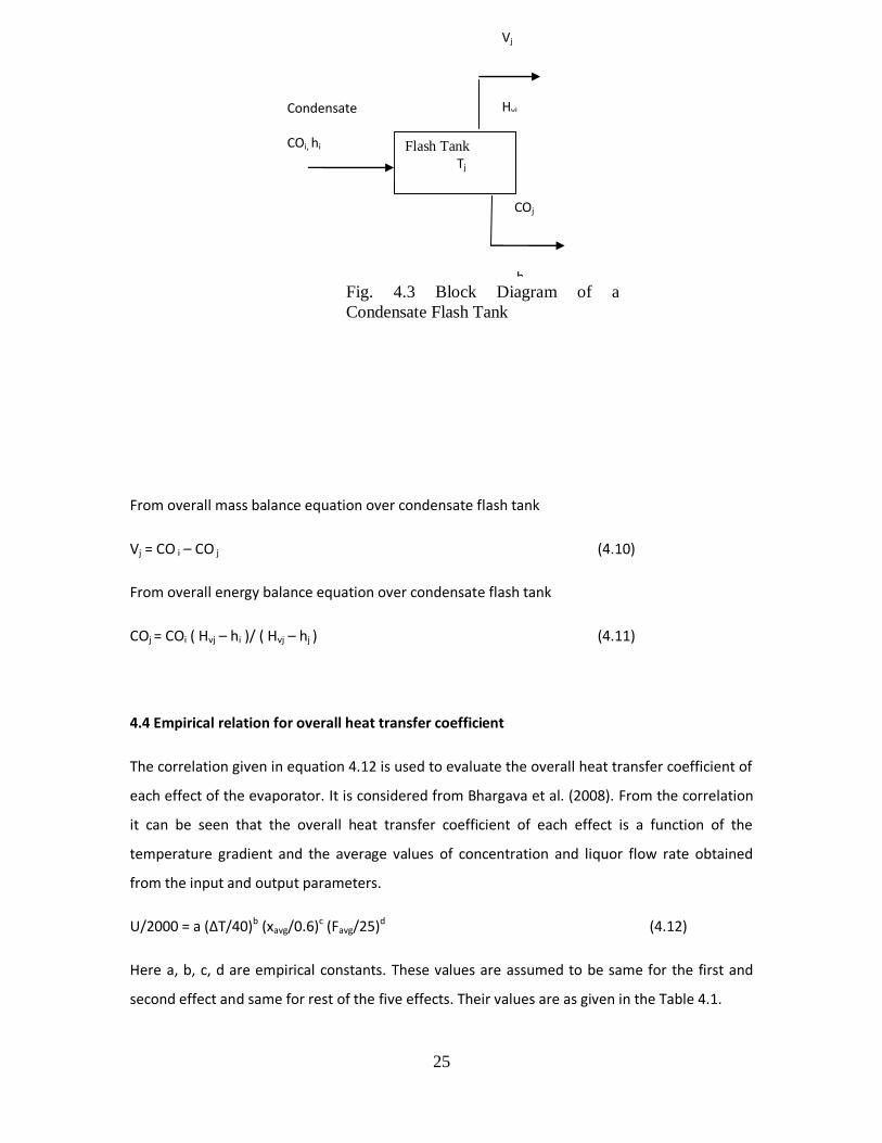
From overall mass balance equation over condensate flash tank

Vj = CO i – CO j (4.10)

From overall energy balance equation over condensate flash tank

COj = COi ( Hvj – hi )/ ( Hvj – hj ) (4.11)

4.4 Empirical relation for overall heat transfer coefficient

The correlation given in equation 4.12 is used to evaluate the overall heat transfer coefficient of

each effect of the evaporator. It is considered from Bhargava et al. (2008). From the correlation

it can be seen that the overall heat transfer coefficient of each effect is a function of the

temperature gradient and the average values of concentration and liquor flow rate obtained

from the input and output parameters.

U/2000 = a (∆T/40)b (xavg/0.6)c (Favg/25)d (4.12)

Here a, b, c, d are empirical constants. These values are assumed to be same for the first and

second effect and same for rest of the five effects. Their values are as given in the Table 4.1.

Flash Tank

Tj

Vj

Hvj Condensate

COi, hi

COj

hj

Fig. 4.3 Block Diagram of a

Condensate Flash Tank

26

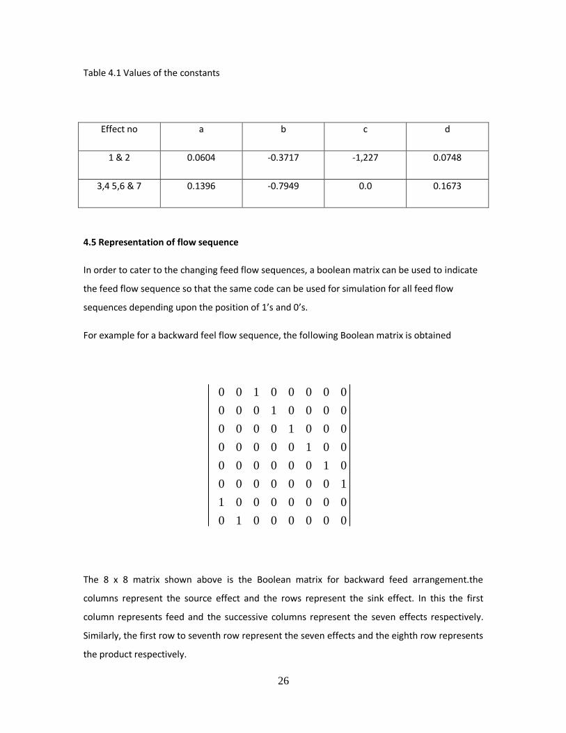
Table 4.1 Values of the constants

Effect no a b c d

1 & 2 0.0604 -0.3717 -1,227 0.0748

3,4 5,6 & 7 0.1396 -0.7949 0.0 0.1673

4.5 Representation of flow sequence

In order to cater to the changing feed flow sequences, a boolean matrix can be used to indicate

the feed flow sequence so that the same code can be used for simulation for all feed flow

sequences depending upon the position of 1’s and 0’s.

For example for a backward feel flow sequence, the following Boolean matrix is obtained

00000010

00000001

10000000

01000000

00100000

00010000

00001000

00000100

The 8 x 8 matrix shown above is the Boolean matrix for backward feed arrangement.the

columns represent the source effect and the rows represent the sink effect. In this the first

column represents feed and the successive columns represent the seven effects respectively.

Similarly, the first row to seventh row represent the seven effects and the eighth row represents

the product respectively.

27

In order to construct the matrix, first the position where the feed is fed is identified, in case of a

backward flow, the feed is fed into the last effect. So for the case considered, the feed is fed to

the seventh effect. Therefore 1 appears in the matrix in the position corresponding to feed

column and seventh effect row. From the seventh effect, the feed goes to the sixth effect,

therefore 1 is written in the matrix in a position corresponding to seventh effect in the column

and sixth effect in the row. Similarly the rest on the Boolean matrix is constructed.

A matlab code is written with the given base case parameters for the given system to find out

the amount of live steam required. The feed and condensate flash tanks are also incorporated

and the amount of auxiliary steam produced by them is calculated to find out the reduction in

steam consumption by the use of flash tanks.

4.6 Generalized model of an effect

In order to simplify the calculation, a generalized model is developed which can be applied for

different operating parameters, for different feed flow sequences and feed, product and

condensate flashing. Fig 4.4 shows the block diagram of ith effect for cascade simulation.(

Bhargava et al. ,2008 )

Fig 4.4 Block diagram of an effect for cascade simulation

ith effect

Vi-1 , T i-1

C i-1

T i-1

Vi

Ti

L i

x i

T Li

L F, x F, y oi (fresh feed)

L j, x j, y ji

Liquor from jth

effect for

J=1,2,…n & j ≠

i

28

The block diagram shown if fig 4.4 shows the generalized diagram of an effect and it can

accommodate any feed flow sequence and can also accommodate the effect of liquor splitting.

Accommodating the effect of flow sequencing and feed splitting the feed flow rate, the black

liquor feed rate to the ith effect can be expressed by the relation given in equation number 4.13

yoi LF + Ljyji (4.13)

In this correlation,

yoi refers to the fraction of feed after feed flashing which enters into the ith effect.

yji refers to fraction of black liquor which comes out from the jth effect and enters into the ith

effect.

Taking these parameters into account, the total mass balance around ith effect can be

represented by equation number 4.14

iijj,i

1j

Fo,i VLLy Lyn

(4.14)

Extending the equation developed for ith effect (equation number 4.14) to an evaporator of n

effects, the matrix representation is as given in fig 4.5

Fig 4.5 Matrix representation of toal mass balance of n effect evaporator

Fonn

Fo33

Fo22

Fo11

n

3

2

1

nn3n2n1n

n3332313

n2322212

n1312111

LyV

:

LyV

LyV

LyV

L

:

L

L

L

1y...yyy

:...:::

y...1yyy

y...y1yy

y...yy1y

This can be represented by

YL = VLF (4.15)

or L = Y-1 VLF = AVLF (4.16)

Here Y matrix is called flow fraction matrix and the matrix A is the inverse of this matrix.

29

From equation number 4.16 the exit liquor flow rate from the ith effect can be expresses as given

in equation number 4.17

ijoj

n

1j

Fjij

n

1j

i ayLVaL (4.17)

The solid mass balance around an effect I can be represented bt the relation given in equation

number 4.18

iijjji

n

1j

FFoi xLxLyxLy (4.18)

Rearranging this equation we get

xLyxLxLy FFoiiijjji

n

1j

Y LX = - Y0 LF xF

Simplifying this the following relation can be obtained

LX = Y-1

(- Y0 LFxF) = - A(- Y0 LFxF)

So, the expression for the total solids coming out of ith

effect can be represented by

equation number 4.19

xL ayxL FFijoj

n

1j

ii (4.19)

Combining equation 4.18 and equation 4.19, an expression for the concentration of liquor

coming out of the ith effect can be determined as given in equation 4.20

i = 2

jij

n

ij

Fijoj

n

1j

ij

n

ij

FFijoj

n

ij

Va)La(y

ax)La(y

(4.20)

We rename the theoretical vapour requirement of each effect Vi-1 as Vbi and then modify

the vapour produced by each effect ( Vi-1 ) by adding to it the vapour produced by feed

30

and condensate flashing. In order to arrive at the exact solution, we have to iterate Vi-1

and Vbi till their values become equal. In order to satisfy this condition we define an

index called Performance Index which can be defined by the equation 4.21 which is a

measure of the difference between Vi-1 and Vbi

PI = ((Vi-1 – Vbi) / Vbi)2 (4.21)

The summation is done for the effects in which live steam is not fed, that is for the given

case from third to seventh effect.

The various parameters of an effect like Ti , TLi , Vi , xi of an effect change with the

pressure (Pi) of the effect bt the change in these parameters is not linear. But assuming

the range of the parameters to be linear, we can approximate these changes to be linear.

As proposed by Stewart and Beveridge (1977) and Ayangbile, Okeke and Beveridge

(1984), it is assumed that vapour produced in a effect Vi is a function of temperature

difference ( i) across the film where i is given by equation number 4.22

Ti = Ti-1 - TLi (4.22)

So writing the relation for the change in Vi with the change in temperature difference we

get,

)Tδ()T(

VδV i

i

ii (4.23)

In this equation, assuming a new variable α such that the expression for α is given by

i)T(

V

i

i

Equation number 4.23 can be rewritten as equation number 4.24

)Tδ( αδV iii )TδT( Li1-ii (4.24)

To determine the relation between the change in Ti with the change in Pi

i

i

ii δP

P

TδT (4.25)

Here defining a variable γ such that the expression for γ is given by

31

γi = i

i

P

T

we can rewrite equation 4.25 as equation 4.26

iii PT (4.26)

From the knowledge that the temperature of the black liquor is a function of the pressure

and the concentration of solids the change in temperature of black liquor can be

expressed as equation 4.27.

iii xδ

x

TδP

P

TδT

i

Li

i

LLi

LiT = i’ Pi + i” xi (4.27)

from equation 4.20, we can get

xi j

n

1j

i δV θ (4.28)

where, i = 2

jij

n

ij

Fijoj

n

1j

ij

n

ij

FFijoj

n

ij

Va)La(y

ax)La(y

Combining equation number 4.27 and 4.28, we get

j

n

ij

iiiLi V δ θδP γδT (4.29)

Defining Vi = Vi-1 - Vbi for i = n, n-1,…,n-ns (4.30)

The changes in Vi-1 and Vbi for the kth iteration can be given by equation 4.31 and 4.32

1-k

1-i

k

1-i1-i VVδV (4.31)

2

jij

n

ij

Fijoj

n

1j

jij

n

ij

FFijoj

n

ij

i

Va)La(y

δVax)La(y

δx

32

1-k

bi

k

bibi VVδV (4.32)

In order to arrive at the solution of the flat falling film evaporator system, the vapour

required for heating by an effect should be equal to the sum of vapour coming out of the

previous effect and the auxiliary vapour added to it from condensate flashing.

bi1-i VV (4.33)

From equation 4.30, 4.31, 4.32 and 4.33 we can obtain

1-ibii δVδVV (4.34)

The vapour required for heating in an effect is a function of vapour produced in that

effect, so on linearization we get relation represented by equation 4.35

i

i

bibi δV

V

VδV

biV ii δV β (4.35)

Combining equations 4.24, 4.26, 4.29, 4.34 and 4.35 and rearranging equation number

4.36 and equation number 4.37 are obtained

s1i1i1ii n-n1,2,..., i re, wheVδV δV (4.36)

0δP γαδP γαδV aθαδV aθα)δaθα(1 iii1-iiijij

n

1ij

iijij

1-i

1j

iiiiiii V

where, i = 1,2,…,n-ns +1 (4.37)

From equation 4.36 and equation 4.37,a set of (2(n-ns) +1) linear algebraic equations with

the same number of unknowns, namely, Vi, where, i = 1,2,…, n-ns+1 and Pi where, i=

1,2,…, n-ns is obtained.

The matrix representation of equation 4.36 and 4.37 can be represented by table 4.2

33

Table- 4.2 Matrix representation of set of linear algebraic equations given by equation 36 and 37

1 - 2 0 0 0 0 0 0 0 0 0 V1 = -

V2

0 1 - 3 0 0 0 0 0 0 0 0 V2 -

V3

0 0 1 - 4 0 0 0 0 0 0 0 V3 -

V4

0 0 0 1 - 5 0 0 0 0 0 0 V4 -

V5

0 0 0 0 1 - 6 0 0 0 0 0 V5 -

V6

1+b11 b12 b13 b13 b15 b16 1 1 0 0 0 0 V6 0

b21 1+ b22 b23 2a24 2 2a25 2 2a26 2 -

2 2

2 2 0 0 0 P1 0

3a31 3 3a32 3 1+ 3a33 3 3a34 3 3a35 3 3a36 3 0 -

3 3 3 3 0 0 P2 0

4a41 4 4a42 4 4a43 4 1+ 4a44 4 4a45 4 4a46 4 0 0 -

4 4 4 4 0 P3 0

5a51 5 5a52 5 5a53 5 5a54 5 1+ 5a55 5 5a56 5 0 0 0 -

5 5

5 5 P4 0

6a61 6 6a62 6 6a63 6 6a64 6 6a65 6 1+ 6a66 6 0 0 0 0 -

6 6

P5 0

40

34

The values for i, i, i and i’ for the different iteration number, denoted by k, are

defined as

For the first iteration, k=1

iii T /V

For the successive iterations, k=2,3…..

αi )T T /()VV( 1k

i

k

i

1k

i

k

i

For the first iteration,k=1

ibii V /V

For the successive iterations, k=2,3…..

βi )V V /()VV( 1k

i

k

i

1k

bi

k

bi

The values of γ and γ’ are given by

i

i

i

ii

i

Li

iP

T

P

)BPR(T

P

T

1-i

1ii

P

T

These values can be obtained from the following correlation

P=0.206-9.89*10-3*T+2.304*10-4*T2-2.03*10-6*T3+1.521*10-8*T4

4.7 Solution technique

Considering the steam pressure in the first and seventh effect and assuming equal pressure drop

across all effects, we will find the pressure in the individual effects. Based on this pressure, we

will calculate the steam and condensate properties for each effect. Using cubic equation 4.9

and finding out its coefficients from equations 4.9a, 4.9b, 4.9c and 4.9d, the liquor outlet from

each effect is found out and from that the concentration of liquor from each effect and the

steam requirement of each effect is also evaluated by material balance and mass balance

35

respectively. After this the auxiliary vapour produced due to condensate flashing is evaluated

and the modified values of vapour produced from each effect is found out which is the sum of

the vapour produced in the effect and the addition vapour produced due to flashing. A

parameter known as performance index is evaluated, which is the difference between the steam

requirement of each effect and the vapour supplied by the preceding effect ( including the flash

vapour). The entire process is iterated till these two values become equal.

4.8 Algorithm

The following algorithm is followed for the matlab code

1. First the following data are read.

Total number of effects.

Number of effects in which live steam is supplied

Inlet concentration of feed

Feed flow rate

Temperature of live steam in the first and second effects

Pressure of steam in the first and last effect

Boolean for the feed flow sequence

Geometrical parameters of the evaporators

2. Assuming equal pressure drop across each effect, the vapour pressure of each

effect is computed from the pressure values of the first and the seventh effect.

These pressure values are used for the initial computation of physical properties of

steam and condensate in each effect.

3. The effect of feed flashing is then evaluated from the inlet concentration and the

feed flow rate. The cubic equation is generated, the coefficients are evaluated and

the outlet liquor flow rate from the feed flash tank is obtained. The outlet liquor

concentration is obtained from component balance. We will set the value of k at 1.

4. Enthalpy of liquor in each effect is evaluated from the empirical relation.

5. The flow rate of liquor from each effect is then evaluated from the cubic equation

and from that the vapour generated from each effect and the outlet concentration

of liquor from each effect is evaluated by mass balance and component balance

36

respectively. Here the vapour generated due to condensate flashing is not taken

into account.

6. New values of xavg and Favg is determined for each effect based on the input and

output parameters of each effect.

7. Then ∆xavg and ∆Favg values are determined.

∆xavg = xavg,new – xavg

∆Favg = Favg,new – Favg

8. If the value of ∆xavg & ∆Favg ≤ 0.0005, we will proceed to next step. If the inequality

is not satisfied, the concentration values of each effect is replaced by the xavg values

and the entire algorithm from step 2 to step 8 is repeated till the inequality is

satisfied.

9. The modified values of overall heat transfer coefficient are found from the

empirical relation given in equation 4.12.

10. The effect of the three primary condensate flash tanks and the four secondary flsh

tanks is evaluated from equations 4.10 & 4.11 and the auxiliary vapour generated

from them is found out. The vapour requirement of each effect is termed as Vbi and

the sum of vapour generated from previous effect and the flash vapour together is

designated as Vi-1 .

11. The performance index of each effect is evaluated which is given by

P ((Vi-1 – Vbi) / Vbi)2

If the PI > 0.001, we will calculate the modified pressure values and repeat steps 2

to 11. If PI < 0.001 , we will end the program.

37

Chapter 5

Results & Discussion

38

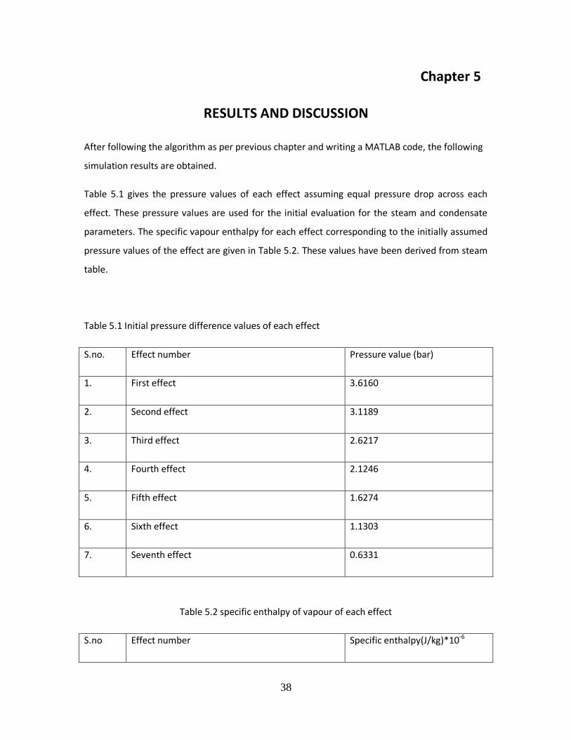
Chapter 5

RESULTS AND DISCUSSION

After following the algorithm as per previous chapter and writing a MATLAB code, the following

simulation results are obtained.

Table 5.1 gives the pressure values of each effect assuming equal pressure drop across each

effect. These pressure values are used for the initial evaluation for the steam and condensate

parameters. The specific vapour enthalpy for each effect corresponding to the initially assumed

pressure values of the effect are given in Table 5.2. These values have been derived from steam

table.

Table 5.1 Initial pressure difference values of each effect

S.no. Effect number Pressure value (bar)

1. First effect 3.6160

2. Second effect 3.1189

3. Third effect 2.6217

4. Fourth effect 2.1246

5. Fifth effect 1.6274

6. Sixth effect 1.1303

7. Seventh effect 0.6331

Table 5.2 specific enthalpy of vapour of each effect

S.no Effect number Specific enthalpy(J/kg)*10-6

39








The feed flow rate is considered from Table 3.1 as 15.55 kg/s with an initial composition of

0.118. Applying the feed flashing on this, the modified liquor flow rate and concentration are

evaluated as

Lmod = 15.2766 kg/s

xmod = 0.1201

Temperature of feed after flashing is given by 53.1˚C

For further calculations, these modified values of inlet liquor flow rate and feed concentration

are considered.

Table 5.3 gives the specific enthalpy of vapour in each effect as evaluated from the empirical

relations

h L = C PP (T L – C 5) J/kg

where,

C PP = C1 ( 1- C4 x)

40

T L = T + τ

τ i = C 3 ( C2 + x i )2

Table 5.3 Specific enthalpy of liquor from each effect

S.no. Effect number Specific enthalpy(J/kg)*10-5








Table 5.4 gives the liquor flow rate from each effect as determined from the cubic equation

given by

a1Li3 + a2Li

2 + a3Li + a4 = 0

where the coefficients are given by

a1 = HVi – C1Ti – C1C22C3 + C1C5

a2 = L i+1 h i+1 + U iA i ( T i-1 – T i – C3C22 ) + L i+1 x i+1 ( C1C4Ti – 2C1C2C3 + C1C3C2

2C4 – C1C4C5 ) – L i+1 H Vi

a3 = ( L i+1 x i+1 )2 ( 2C1C2C3C4 - C1C3 ) – 2 C2C3UiAi L i+1 x i+1

a4 = ( C1C3C4 L i+1 x i+1 – C3UiAi ) (L i+1 x i+1 )2

The real root of the cubic equation is given by

L = -a2/(3a1) + ((P13 + Q1

2)1/2 – Q1)1/3 – ((P13 + Q1

2)1/2 + Q1)1/3

41

Where,

P1 = a3/(3a1)-(a2/(3a1)2

Q1 = (a4 – a23/(27a1

2) – a2 P1)

It also gives the liquor composition as obtained from component balance and the outlet vapour

flow rate from each effect as obtained from mass balance. Since the multiple effect evaporator

system considered is of backward flow arrangement, therefore the values are tabulated in

reverse order. After obtaining the initial values, the check condition of ∆xavg & ∆Favg. After

satisfying the condition, the final values obtained are as follows.

Table 5.4 liquor flow rate, concentration and vapour flow rate from each effect

S.no. Effect number Liquor flow rate

(kg/s)

Liquor

Concentration

Vapour flow rate

(kg/s)

1. Seventh effect 14.0884 0.1312 2.3764

2. Sixth effect 11.8993 0.1553 2.0018

3. Fifth effect 10.0289 0.1843 1.7391

4. Fourth effect 8.4401 0.2190 1.4386

5. Third effect 7.1770 0.2571 1.0877

6. Second effect 6.2396 0.2953 0.7871

7. First effect 5.7752 0.3178 0.1416

42

The value of steam from each effect given in table 5.4 does not include the effect on condensate

flashing. After incorporating the effect of three primary flash tanks and four secondary flash

tanks, the modified values of vapour produced from each effect is evaluated. These values are

1

2

3

4

5

6

7

FFT

15.55

0.118

15.27

15.27

0.1201

14.0884

0.1312

11.8993

0.1553

10.0289

0.0289

0.184

3

8.4401

0.2190

7.177

0.2571

0.257

1

6.2396

0.2953

0.2953

5.7752

0.3178

0.1416 0.7871 1.0877 1.4386 1.7391 2.0018 2.3764

43

the sum of the values of vapour produced from the preceding effect and the vapour generated

from the condensate flash tanks.

Table 5.5 gives the amount of vapour generated from each of the condensate flash tanks

Table 5.5 Vapour generated from flash tanks

S.no. Flash tank number Amount of vapour (kg/s)

1. CF V1 0.0063

2. CF V2 0.0103

3. CF V3 0.0153

4. CF V4 0.0029

5. CF V5 0.0083

6. CF V6 0.0182

7. CF V7 0.0369

These values of vapour generated from the condensate flash tanks are added to the respective

streams of vapour generated from each of the effects and the modified values of vapour

generated from each effect is evaluated in table 5.6

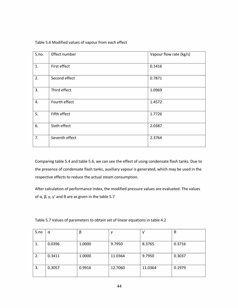
44

Table 5.6 Modified values of vapour from each effect

S.no. Effect number Vapour flow rate (kg/s)








Comparing table 5.4 and table 5.6, we can see the effect of using condensate flash tanks. Due to

the presence of condensate flash tanks, auxiliary vapour is generated, which may be used in the

respective effects to reduce the actual steam consumption.

After calculation of performance index, the modified pressure values are evaluated. The values

of α, β, γ, γ’ and θ are as given in the table 5.7

Table 5.7 Values of parameters to obtain set of linear equations in table 4.2

S.no α β γ γ' θ

1. 0.0396 1.0000 9.7950 8.3765 0.3716

2. 0.3411 1.0000 11.0364 9.7950 0.3037

3. 0.3057 0.9916 12.7060 11.0364 0.1979

45

4. 0.2885 0.9872 15.0803 12.7060 0.1175

5. 0.2578 0.9811 18.7592 15.0803 0.0628

6. 0.2129 0.9819 25.3314 18.7592 0.0296

The matrix A is the inverse of matrix Y

A = -1 -1 -1 -1 -1 -1 -1

0 -1 -1 -1 -1 -1 -1

0 0 -1 -1 -1 -1 -1

0 0 0 -1 -1 -1 -1

0 0 0 0 -1 -1 -1

0 0 0 0 0 -1 -1

0 0 0 0 0 0 -1

The modified pressure values as obtained by solving the set of linear equations given in table

4.2, after the first iteration is as given in table 5.8. These values of pressure are used in the

successive iteration for the calculation of steam and condensate properties.

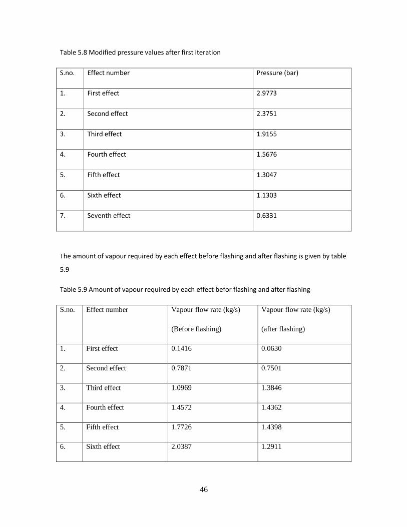
46

Table 5.8 Modified pressure values after first iteration

S.no. Effect number Pressure (bar)








The amount of vapour required by each effect before flashing and after flashing is given by table

5.9

Table 5.9 Amount of vapour required by each effect befor flashing and after flashing

S.no. Effect number Vapour flow rate (kg/s)

(Before flashing)

Vapour flow rate (kg/s)

(after flashing)

1. First effect 0.1416 0.0630

2. Second effect 0.7871 0.7501

3. Third effect 1.0969 1.3846

4. Fourth effect 1.4572 1.4362

5. Fifth effect 1.7726 1.4398

6. Sixth effect 2.0387 1.2911

47

7. Seventh effect 2.3764 2.3061

The final steam consumption for the given system of seven effect evaporators is given by 7056.0

kg/hr after flash tanks are incorporated and the steam consumption before the flash tanks are

incorporated is given by 7488.0 kg/hr.

48

Chapter 6

Conclusion

49

Chapter 6

CONCLUSION

In the present work, cascade simulation of a flat falling film seven effect evaporator system is

done in order to optimize the system in terms of live steam requirement of the system. A

generalized solution technique is used so that the same algorithm and code could be used and

there be no need for a separate code for the different feed flow sequences or when additional

flash tanks are used. Taking the results into account, the conclusions that can be drawn from the

work are that the presence of flash tanks in a multiple effect evaporator system helps in reducing

the live steam requirement of the system by deriving heat from the vapour as well. In the

present work, initially the live steam requirement of the system is evaluated without the

presence of any flash tanks and it is found out to be and the live steam requirement of the

system is evaluated in the presence of seven condensate flash tanks and one feed flash tank.

The live steam requirement of the system without the use of flash tanks is found to be 7488.0

kg/hr

And with the use of flash tanks is found to be 7056.0 kg/hr .

The reduction in the consumption of live steam is because of the derivation of heat from the

vapour coming out of each effect and it is found to be 432 kg/hr. This reduces the live steam

consumption of the multiple effect evaporator system and hence the process is economized in

terms of live steam consumption.

50

REFERENCES

1. R. Bhargava , S. Khanam , B. Mohanty , A.K. Ray, (2008) “Simulation of flat falling film evaporator

system forconcentration of black liquor”, Computers and Chemical Engineering 32 3213–3223.

2. R. Bhargava , S. Khanam, B. Mohanty, A.K. Ray, (2008) " Selection of optimal feed flow sequence

for a multiple effect evaporator system” , Computers and Chemical Engineering 32 2203–2216

3. McCabe Smith Harriot , Unit Operations in Chemical Engineering, Mc Graw Hill.

4. Radovic, L. R., Tasic, A. Z., Grozanic, D. K., Djordjevic, B. D., & Valent, V. J. (1979), Computer

design and analysis of operation of a multiple effect evaporator system in the sugar industry.

Industrial and Engineering Chemistry Process Design and Development, 18318–323.

5. Ray, A. K., Rao, N. J., Bansal, M. C., &Mohanty, B. (1992), Design data and correlations of waste

liquor/black liquor from pulp mills. IPPTA Journal, 4 1–21.

6. Ayangbile, W. O., Okeke, E. O., & Beveridge, G. S. G. (1984). Generalised steady state cascade

simulation algorithm in multiple effect evaporation.Computers & Chemical Engineering, 8, 235–

242.

7. Bhargava, R. (2004). Simulation of flat falling film evaporator network. PhD dissertation,

Department of Chemical Engineering, Indian Institute of Technology Roorkee, India

8. Bremford, D. J., & Muller-Steinhagen, H. (1994). Multiple effect evaporator performance for

black liquor. I. Simulation of steady state operation for different evaporator arrangements.

Appita Journal, 47, 320–326.

9. El-Dessouky, H. T., Alatiqi, I., Bingulac, S., & Ettouney, H. (1998). Steady state analysis of the

multiple effect evaporation desalination process. Chemical Engineering & Technology, 21, 15–29.

10. El-Dessouky, H. T., Ettouney, H. M., & Al-Juwayhel, F. (2000). Multiple effect

evaporation–vapor compression desalination processes. Transactions of the IChemE, 78(Part A),

662–676.

11. Holland, C. D. (1975). Fundamentals and modelling of separation processes. Englewood Cliffs, NJ:

Prentice Hall Inc.

12. Itahara, S.,&Stiel, L. I. (1966). Optimal design of multiple effect evaporators by dynamic

programming. Industrial&Engineering Chemistry Process Design and Development, 5, 309.

13. Lambert, R. N., Joye, D. D., & Koko, F. W. (1987). Design calculations for multiple effect

evaporators. I. Linear methods. Industrial & Engineering Chemistry Research, 26, 100–104.

14. Nishitani, H.,&Kunugita, E. (1979). The optimal flow pattern of multiple effect evaporator

systems. Computers & Chemical Engineering, 3, 261–268.

51

15. Mathur, T. N. S. (1992). Energy conservation studies for the multiple effect evaporator house of

pulp and paper mills. PhD dissertation, Department of Chemical Engineering, University of

Roorkee, India.

optimization of a multiple effect evaporator system - ethesis

Documents