FOXES TEAM Tutorial on Numerical Analysis with Optimiz.xla

Optimization, Nonlinear Fitting

and Equations Solving

Volume

1O

T U T O R I A L O N N U M E R I C A L A N A L Y S I S F O R O P T I M I Z . X L A

Optimization, Nonlinear Fitting and Equations Solving

T U T O R I A L F O R M A T R I X . X L A

2

Index OPTIMIZ.XLA ..........................................................................................................................4 Optimiz.xla installation.............................................................................................................5

How to install ......................................................................................................................................5 How to uninstall ..................................................................................................................................6

Optimization...............................................................................................................................8 Optimization "on site"...............................................................................................................8 Optimization strategy...............................................................................................................9 Optimization algorithms .........................................................................................................10 Algorithms Implemented In This Addin..................................................................................11 The starting point ...................................................................................................................12 Optimization Macros ..............................................................................................................14

Derivatives (Gradient).......................................................................................................................14 Optimization Macros with Derivatives...............................................................................................15 The Input Menu Box: ........................................................................................................................15 Optimization Macros without Derivatives ..........................................................................................16

Examples Of Uni-variate Functions .......................................................................................18 Example 1 (Smooth function) ...........................................................................................................18 Example 2 (Many local minima)........................................................................................................19 Example 3 (The saw-ramp) ..............................................................................................................20 Example 4 (Stiff function)..................................................................................................................20 Example 5 (The orbits) .....................................................................................................................22

Examples of bi-variate functions............................................................................................24 Example 1 (Peak and Pit) .................................................................................................................24 Example 2 (Parabolic surface)..........................................................................................................25 Example 3 (Super parabolic surface) ...............................................................................................26 Example 4 (The trap) ........................................................................................................................27 Example 5 (The eye) ........................................................................................................................30 Example 6 (Four Hill) ........................................................................................................................30 Example 7 (Rosenbrock's parabolic valley) ......................................................................................31 Example 8 (Nonlinear Regression with Absolute Sums)...................................................................33 Example 9 (The ground fault) ...........................................................................................................35 Example 10 (Brown bad scaled function) .........................................................................................35 Example 11 (Beale function).............................................................................................................36

Examples of multivariate functions ........................................................................................37 Example 1 (Splitting function method) ..............................................................................................37 Example 2 (The gradient condition)..................................................................................................38 Example 3 (Production) ....................................................................................................................39 Example 4 (Paraboloid 3D)...............................................................................................................40

LP - Linear programming.......................................................................................................41 LP - Linear programming ..................................................................................................................41

Optimization with Linear Constraints .....................................................................................43 NLP with linear constraints ...............................................................................................................43

Nonlinear Regression .............................................................................................................46 Nonlinear Regression for general functions ..........................................................................48

Levenberg-Marquardt macro ............................................................................................................48 Nonlinear Regression with a predefined model.....................................................................51

T U T O R I A L F O R M A T R I X . X L A

3

Example 1 (Exponential class) .........................................................................................................52 Example 2 (Exponential Class).........................................................................................................54 Example 3 (using derivatives)...........................................................................................................57 Example 4 (Rational class) ...............................................................................................................59 Example 5 (Multi variable regression) ..............................................................................................60

Gaussian regression..............................................................................................................61 Rational regression................................................................................................................63 Exponential regression ..........................................................................................................66

Simple Exponential model ................................................................................................................66 Offset ................................................................................................................................................69 Multi-exponentials model ..................................................................................................................70 Good fitting is good regression ? ......................................................................................................71

Damped cosine regression....................................................................................................72 Power regression...................................................................................................................73 Logarithmic regression ..........................................................................................................74 NIST Certification Test...........................................................................................................75

Nonlinear Equations Systems ...............................................................................................76 Nonlinear Equations Systems ...............................................................................................76 NL Equation macros ..............................................................................................................77

NLE - Newton-Raphson....................................................................................................................78 NLE - Broyden ..................................................................................................................................80 NLE - Brown .....................................................................................................................................82 NLE - Global rootfinder .....................................................................................................................84 Univariate Rootfinding macro ...........................................................................................................90 2D - Zero Contour.............................................................................................................................92 2D Intersection .................................................................................................................................95

Credits ......................................................................................................................................97

References ...............................................................................................................................97

4

About this tutorial OPTIMIZ.XLA OPTIMIZ for Microsoft EXCEL contains macros to perform the optimization of multivariable functions. This add-in contains also several routines for nonlinear regression and nonlinear equation solving, the important tasks, strictly related to the optimization one. Except in linear cases, optimization proceeds by iterations. Starting from an approximate trial solution an algorithm will gradually refine the working estimate until a prefixed precision has been reached. In this add-in you can find a few algorithms covering different kind of optimization problems. All of them are realized by Excel macros and can be activated from the menu: "Tools ⇒ Optimiz ..." They work "on-site". It means that the macros work directly on the cells of your worksheet where you have defined the function to optimize. They have been developed mainly with the aim of teaching the most popular optimization algorithms and their related methods. But, of course, they are also useful in practical real problems of low-moderate dimension. Algorithms covered by this tool are: Nelder-Mead Downhill-Simplex, Newton-Raphson, Levenberg-Marquadt least squared fitting, Conjugate-Gradient, Davidon-Fletcher-Powell, Broyden, Brown, Montecarlo, etc. The main purpose of this document is to show how to work with the Optimiz.xla add-in for solving non-linear regression and optimization problems. Of course this speaks about math, statistic and numeric calculus but this is not a math or a statistic book. Therefore, you will rarely find theorems and demonstrations. You will find, on the contrary, many examples that explain, step by step, how to reach the result that you need, straight and easy. And, of course, we speak about Microsoft Excel but this is not a tutorial on Excel. Tips and tricks for general applications in Excel can be found at many internet sites.

I am grateful to all those who will provide constructive criticisms. Leonardo Volpi

Chapter

1

5

Optimiz.xla installation The OPTIMIZ add-in for Excel 2000/XP is a zip file composed of two files:

• OPTIMIZ.XLA Excel add-in file • OPTIMIZ.HLP Help file

It is available as a download from the website http://digilander.libero.it/foxes/SoftwareDownload.htm,

under the title “Didactic Optimization Tool for EXCEL” as “Optimiz tool.zip” in blue. How to install Unzip and place all the above files in a directory that is accessible by Excel. The best choice is in the Add-ins directory which is in the following sequence

Local Disk (C: or something else)

Documents & Settings

(Your name, which is a directory that comes up on startup)

Application Data

Microsoft

Addins.

When loaded/saved, the add-in is contained entirely in this directory. Your system is not modified in any other way. If you want to uninstall this package, simply delete the designated files - it's as simple as that!.

To install in Excel as a menu item, follow the usual procedure for installing a “*.xla” add-in to the main menu.

1) Open Excel

2) From the Excel menu toolbar select "Tools" and then select "Add-ins".

3) If “optimization tool” does not appear in the list, Optimize.xla has not been linked in, Select the Browse box on the right side of the list, and the above Addins directory will appear. (If you loaded it into some other place, you will have to search for it.) Select optimize.xla.

4) Once in the Add-ins Manager list, look in the list for “optimization tool” and select it

5) Click OK

After the first installation, OPTIMIZ.xla1 will be added to the Add-in list manager as ‘optimization tool’. Your Addin Manager list will appear differently from the one shown below (on the left side). The lists will be different depending on which foreign language version of Excel you are using and what other tools you are using. When Excel starts, all add-ins checked in the Add-ins Manager will be automatically loaded. If you want to stop the automatic loading of OPTIMIZ.xla, simply deselect the check box next to “optimization tool” before closing Excel.

1 This tutorial has been written for users of the English version of Excel The illustrations of the appearance of Excel when Optimize.xla is used are from the Italian version of Excel. These illustrations were not changed, since the version used by the author and the Foxes team is the Italian version.

6

If the installation is correct,, you should see the welcome popup of OPTIMIZ.xla. This appears only when you select "on" the check box of the Addin Manager. When Excel automatically loads OPTIMIZ.xla, this popup remains hidden. How to uninstall This package never alters your system files

If you want to uninstall this package, simply delete the file. Once you have cancelled the OPTIMIZ.xla file, to remove the corresponding entry in the Addin Manager list, follow these steps:

1) Open Excel

2) Select <Addins...> from the <Tools> menu.

3) Once in the Addins Manager, click on ‘optimization tool’.

4) Excel will inform you that the addin is missing and ask you if you want to remove it from the list. Select "yes".

7

WHITE PAGE

8

Optimization Optimization Optimization "on site" Optimiz was developed for performing the optimization task directly on a worksheet. This means that you can define any relationship that you want to optimize, simply by using the standard Excel built-in functions and your equations that relate them. The optimization macros will update directly the cells containing the parameters to be changed and the related variables to be optimized. Object function. For example: if you want to search for the minimum of the bi-dimensional function

( ) ( )2100352

10051),( −+−= yxyxf

, you insert in the cell E4 the formula "=(B4-0.51)^2+(C4-0.35)^2". Here the cells B4 and C4 contain the current values of the variables x and y. By changing the values of B4 or C4, the function value E4 is also consequently changed.

Gradient. Some optimization algorithms require the gradient of the function, which is the derivative with respect to each independent variable. In that case you must insert also the gradient formulas. In our simple case we have for the gradient:

( ) ( )( )10035

10051 2 , 2 , −−=

∂∂

∂∂

=∇ yxyf

xff

Chapter

2

9

Constraints. Usually constrained variables have simple bounding constraints (for example, as follows):

11 , 11 <<−<<− yx On the worksheet these constraints are arranged in a rectangular range (2 x n) where the first row contains the lower limits and the second row the upper limits.

Doing an optimization using worksheet cells and cell equations is slower than by doing it with VBA subroutines that use the worksheet only for the input data and output parameters. The former method gives considerable flexibility, but is prone to errors. The latter method is inflexible, but errors are much reduced Optimization strategy In numerical analysis the optimization of a function is not a trivial task and there is no single algorithm good for all cases. Each time it is to be done, we have to study the problem to establish an optimization strategy by choosing: :

• The most adapt algorithm

• The most adapt starting point

The algorithm depends strongly on the characteristics of the function that we have to optimize. The choosing of the starting point depends on the local behavior near the "optimum" of the function itself.

10

Optimization algorithms The best optimization algorithm, good for every case, is unknown, and this should be obvious. However, there are several good algorithms adapted for large cases of practical common optimization problems, from which one can be selected. Generally speaking we have to choose between algorithms that use derivatives (Gradient) and those that do not. In general, methods that use derivatives are the more powerful and accurate. However, the increase in speed does not always outweigh the extra overhead in computing the derivatives. Sometime, it is also impossible or impractical to calculate exactly the derivatives . There are also cases in which the derivative information is useless. This happens for discontinuous or quasi-discontinuous functions.

here, methods with gradient are better

here, methods without gradient are better

Also, the local behavior near the optimum can favor one type of algorithm instead of others. It happens for example, when there is a narrow extreme point near other local extremes or, at the opposite, when the function has a large flat "valley".

Here, methods with gradients are more efficient.

Here, methods without gradients are able to arrive at a global optimum and not hang-up at a local optimum.

11

Algorithms Implemented In This Addin Downhill-Simplex The Nelder–Mead downhill simplex algorithm is a popular derivative-free optimization method. It is based on the idea of function comparisons among a simplex of N + 1 points. Depending on the function values, the simplex is reflected or shrunk away from the maximum point. Although there are no theoretical results on the convergence of the algorithm, it works very well on a wide range of practical problems. It is a good choice when a one-optimum solution is wanted with minimum programming effort. It can also be used to minimize functions that are not differentiable, or that we cannot differentiate. It shows a very robust behavior and converges over a very large set of starting points. In our experience it is the best general purpose algorithm; solid as a rock. It's a "jack of all trades”.

Random This is another derivative-free algorithm. It simply "shoots" a set of random points and takes the best extreme value (max or min). Usually the accuracy is not comparable with the other algorithms (only about 5%), and it also requires a considerable extra effort and time. On the other hand, it's absolutely insensitive to the presence of unwanted local extremes, and works with smooth and discontinues functions as well. In this implementation, the random algorithm can increase the accuracy (0.01%) by a "resizing" strategy (under particular conditions of the objective function). On the contrary, this algorithm is not adaptable for functions that have a large "flat" region near the extreme, like what happens in the least squared optimization. Convergence problems do not exist because a starting point is not necessary

Divide-Conquer 1D For univariate functions only. It's another very robust, derivative free algorithm. It is simply a modified version of the bisection algorithm. It can be adapted to every function, smooth or discontinuous. It converges over a very large segment of parameter space.

Parabolic 1D For univariate functions only. This algorithm uses a parabolic interpolation to find any local extreme (maximum or minimum). It is very efficient and fast with smooth-derivable functions. The starting point is simply a segment of parameter space bracketing the extreme (local or not) that we want to find. The condition is that the extreme must be within the stated segment.

Conjugate Gradients Also called CG. This is a very popular algorithm that cannot miss. It requires a gradient evaluation at each step which can be approximated internally by the finite difference method or supplied directly by the user as well. The exact gradient information improves the accuracy of the final result, but in many case these differences are not relevant to the extra effort. The starting point should be chosen sufficiently close to the optimized one.

Davidon-Fletcher-Powell Also know as DFP algorithm. This is a sophisticated and efficient method for finding extremes of smooth-regular functions. It requires a gradient evaluation at each step which can be approximated internally by the finite difference method or supplied directly by the user as well. The exact gradient information improves the accuracy of the final result, but in many case these

12

differences are not relevant to the extra effort. The starting point should be chosen sufficiently close to the optimized one, even if the region is larger than the allowable region for a CG solution. Newton-Raphson The most popular algorithm for solving nonlinear equations. It needs the exact gradient for approximating the Hessian matrix. It is extremely fast and accurate but, because of its poor global convergence performance, it is used only for refining the final result from another algorithm.

Levenber-Marquardt Levenberg-Marquardt is a popular alternative to the Gauss-Newton method of finding the minimum of a function that is a sum of squares of nonlinear functions. This algorithm was found to be an efficient, fast and robust method which also has a good global convergence property. For these reasons, It has been incorporated into many good commercial packages performing non-linear regression. Finding this algorithm on public domain is not very easy. .

The starting point Almost all optimization algorithms require a starting point. It is a set of initial values of the independent variables from which the algorithm begins its searching. A "good" starting point is very important to obtain a good optimization result. Sometime the convergence fails; sometime the algorithm converges to a local minimum or a local maximum, which in general, is not the optimum. Many times these traps can be avoided by choosing an "adapt" type of starting point. How can we choose a "good" starting point? We have to say that this is the key of any optimization problem. Before starting the optimization, we have to study the objective function, acquiring as much information as possible about the function itself and, if possible, also about its derivatives. We have to guess how the function grows or decays and where the locations are (if any) of the "valleys" and "mountains" of the function itself. The most solid method for this, is function plotting. For one-dimensional functions f(x) we simply plot the function itself. Choosing an adapt scale factor and a zoom window we are sure to bracket the location of the desired minimum and maximum.

For two-dimensional functions f(x, y) we can plot the contour-lines for several different function values.

13

Example of contour-lines plots

We can also plot a 3D graph but it is less useful, in our opinion, then the contour-lines method. Anyways, there are lots of good programs, also freeware that perform this task. An example of good 3D plots

If you like, with a little patience, you can construct a similar graph also in Excel. Alternatively you can download the freeware workbook Random_Plot.xls from our website that just creates automatically a 3D plot and a contours plot of two-dimensional functions. Example of the graph obtained with Random_Plot.xls

14

This example shows that the starting point for searching the function minimum should be taken in the half triangular domain where the hole is located. On the contrary, it would be inefficient to start with a point located behind the big mountain. Simply, imagine a little ball rolling along the surface. Where from, do you think it can quickly fall into the hole? For functions having more than 2 dimensions, the difficulty increases sharply because we cannot use the plot method as it is. We have to plot the graphs of several function sections. We keep fixed a variable (for example z) to one value (for example 1) and then plot the function f(x, y, 1) as a contour lines plot. This plot is a section (or "slice") at z = 1 of the function f(x, y, z). Repeating for several values of z with can map the behavior of the entire function Optimization Macros According to the didactic intention of this add-in, the macros are named with the algorithm's name instead with the usual scope or action of the macros themselves We could say that the scope is always the same: finding the optimized point of a given function. What mainly differentiates each macro is its action field. For example the Levenberg-Marquardt algorithm is generally the most adapt for the nonlinear least squared fitting; but many times we can see that the Downhill-Simplex algorithm is competitive. The Downhill-Simplex algorithm is sometimes superior, due to its robust global convergence property. In other words: "there is no any fixed situation" and each problem must be always studied before attempting to find the optimum. Derivatives (Gradient) A primary decision is the choice between algorithms using derivatives or algorithms without derivatives. One thinks that the second choice is automatic when the derivative is unknown or too hard to calculate. The second choice is not always a valid choice, because the algorithms could easily approximate internally the derivatives with sufficiently accuracy. The reason why the primary decision about derivatives is deeper comes from the basic nature of the function. When we adopt to algorithm that uses the gradient we should be sure that this information is valid and will remain valid in the working domain of the function. This happens not for all functions. Analytical, smooth, functions like polynomials and exponentials fulfill this rule; and also rational, power and logarithmic functions when the domain does not include singularity. Using derivatives can greatly improve both accuracy and convergence speed. So, in general, algorithms that use derivatives are very fast.

There are cases, on the contrary, where derivative information is not useful or will even hinder the convergence. This happens for discontinuous functions or for discontinuous derivatives. In these cases is better to ignore the derivative information. Another case happens when the function has many local extremes near the optimum one; in this case, following the derivative information, the algorithm might fall into one of the "traps" of local extremes.

15

Optimization Macros with Derivatives Those macros need information about:

1. The cell containing the definition (computed result) of the function to optimize (objective function)

2. The range of the cells containing the values (variables) to be changed (max 9 variables)

3. The range containing the constraints (minimum and maximum limits) on the variables (constraints box)

4. Optionally the range of the values of the computed gradient functions, one for each variable.

The locations of the cells within each of these ranges must be consistent with the specific variables, so that there is a direct, unambiguous link to all the required information about each variable. If the arrangement on the worksheet mixes up the relationships, then the computation may fail or be entirely wrong.

The Input Menu Box:

1. Select ‘Tools’ from the uppermost Excel menu list

2. Select the ‘f(x) optimization’ line

3. Another box will appear. Select the desired method.

4. For the ‘Conjugate-Gradient’ method, the following data entry box will appear. The other methods have similar data input boxes.

16

Maximum or Minimum Selection: The two buttons in the upper right of the menu box switch between the minimization and maximization algorithms Gradient: If the gradient formulas are provided (the range entered) the macro will use them for its internal calculations. Otherwise the derivatives are approximated internally by the finite difference central formulas. Newton-Raphson Option: If checked, the macro will attempt to refine the final result with 2-3 extra iterations of the Newton-Raphson algorithm. This option always requires the gradient formulas, for evaluating the Hessian matrix with sufficient accuracy to obtain a good optimum value. It is a numerical problem, inherent in the loss of accuracies of the differences obtained by numerical subtractions. Stopping Limit. In each panel there is always an input box for setting the maximum number of iterations or the maximum number of evaluation points allowed. The macro stops itself when this limit has been reached. Relative Error Limit: In the "Random" macro there is also an input box for setting the relative error limit. The other algorithms do not use the error criterion, they simply stop when the accuracy does not increase anymore after several iterations. Optimization Macros without Derivatives Those macros need information only about:

1. The cell containing the definition (computed result) of the function to optimize (objective function)

2. The range of the cells containing the values (variables) to be changed (max 9 variables)

3. The range containing the constraints (minimum and maximum limits) on the variables (constraints box)

The locations of the cells within each of these ranges must be consistent with the specific variables, so that there is a direct, unambiguous link to the specific constraint.

17

If the arrangement on the worksheet mixes up the relationships, then the computation may fail or be entirely wrong.

Maximum or Minimum Selection: The two buttons in the upper right of the menu box switch between the minimization and maximization algorithms Stopping Limit. In each panel there is always an input box (Points) for setting the maximum number of iterations or the maximum number of evaluation points allowed. The macro stops itself when this limit has been reached. Relative Error Limit: In the "Random" macro there is also an input box for setting the relative error limit. The other algorithms do not use the error criterion, they simply stop when the accuracy does not increase anymore after several iterations.

18

Examples Of Uni-variate Functions

Example 1 (Smooth function) The search for an extreme in a uni-variate smooth function is quite simple and almost all algorithms usually work. We have only to plot the function to locate immediately the extreme. Assume for example, a problem of finding a local maximum and minimum of the following function in the range 0 < x < 10

21)sin()(xxxf

+=

The plot below shows that there are three local extreme points within the range of 0 to 10.

Interval Extreme 0 < x < 2 local max that is also the absolute max

2 < x < 6 local min that is also the absolute min

6 < x < 10 local max In order to approximate the extreme points we can use the parabolic interpolation macro. This algorithm converges to the extreme within each specified interval, no matter if it is a maximum or a minimum. A possible worksheet arrangement may be the following where the range A3:B3 is the constrain box, the cell C3 is the variable to change, and the cell D3 contains the function

Repeating the search for each interval we find

19

a b x f(x) 0 2 1.109293102 0.5995221642 6 4.503864793 -0.21205764 6 10 7.727383943 0.127312641

If we want to find the absolute maximum or minimum within a given interval we must use the divide-and-conquer algorithm (a variant of the bisection algorithm)

Example 2 (Many local minima) An optimization algorithm may give a wrong result when there are too many local extremes (minimum and maximum) near the desired absolute maximum or minimum. In that case they can be trapped into one of the local extremes. For example assume to have to find the maximum and minimum of the following function within the range, 0 < x < 5

)6cos()( xexxf x ⋅⋅= −

In the range 0 < x < 5 there are many local minimum and maximum points. We could bracket the absolute maximum within a small interval before starting the searching algorithm. But we want to show the evidence that the Divide-and-Conquer algorithm, (thanks to its intrinsically robustness) can escape the local "traps" and give the correct absolute max and min Starting the macro "1D Divide and Conquer"

20

a b x f(x) max 0 5 1.0459 0.367 min 0 5 1.5608 -0.327

As we can see the algorithm ignores the other local extremes and converges to the true absolute maximum. But of course this is a didactic extreme case. Generally speaking, it is always better to isolate the desired extreme within a sufficiently close segment before attempting to find the absolute maximum (minimum). If it's impossible and there are many local extremes, you may increase the number of points limit from 600 (default) to 1000 or 2000. Example 3 (The saw-ramp) This example illustrates a case quite difficult for many optimization algorithms, even if it is quite simple to find the maximum and minimum by inspection of a plot of the function. Assume we have to search the maximum and minimum for a function shown in the plot, in the range 0 < x < 4 Its analytical expression, quite complicated, is:

( ) 1|int|4||)( 21 +−+⋅+= xxxxf

The optimization macro will converge to the point (0, 1) for the minimum and to (3.5, 6.5) for the maximum

Example 4 (Stiff function) This example shows another difficult function. The concept of stiff functions is similar to the differential equation problem: We are speaking of stiff problems when the function evolves smoothly and slowly in a large interval except in one or more small intervals where the evolution is more rapid. Usually this kind of function needs two or more plots with different scales. Given the following function for x ≥ 0 , find the absolute max and min

( )21

sin)(xxxf

+=

For a good study, this function requires two plots

21

One plot covers the wide range 0 < x < 100 and another covers the smaller region 0 < x < 10 where the function shows a narrow maximum. (Note that there are other local extremes within the global interval.) The absolute minimum is located within the interval 10 < x < 30. For finding the maximum and minimum with the best accuracy, we can use the divide-and-conquer algorithm (robust convergence), obtaining the following result:

a b x f(x) rel.error 0 100 18.2845204 -0.049492601 6.97E-09 0 100 0.760360454 0.6094426 2.23E-08

Note that the parabolic algorithm has some convergence difficulty in finding the maximum near 0, if the interval is not sufficiently close to zero. On the contrary, there is no problem for the minimum

a b x f(x) rel.error 0 3 6.869565509 0.07165213 6.11E+00 0 2 -1.668589413 #NUM! -

0.5 1.5 0.760360472 0.6094426 2.72E-10 10 30 18.28452054 -0.04949260 1.00E-09

This behavior for the ranges near zero, can be explained by observing that the function does not have a derivative value at x = 0. The derivative is:

( ) ( ) ( )( )32

32

12

sin2cos1)('xx

xxxxxf+⋅

−+=

which at x=0 is infinite.

22

Example 5 (The orbits) The objective function also can have an indirect link to the parameter that we have to change. This is illustrated in the following example: Two satellites follow two plane elliptic orbits described by the following parametric equations with respect to the earth.

−=+=

≡)cos()sin(4

)sin(3)cos(2SAT1

ttyttx

=+=

≡)sin(

)sin(2)cos(SAT2

tyttx

For time t = 0 the two satellites stay at positions (2, −1), (1, 0) respectively

We want to find when the two satellites have a minimum distance from each other (In order to transmit messages with the lowest noise possible). We want to also find the position of each satellite at the minimum distance. (Note that, in general, this position does not coincide with the static minimum distance between the orbits.) This problem can be regarded as a minimization problem having one parameter (the time "t") and one objective function (the distance "d") The distance on a plane between two points is

( ) ( )2212

21 yyxxd −+−= We can solve this problem directly on a worksheet as shown in this example.

Range B4:C5: The x and y coordinates of the two satellites at a given time. Range E4: Parameter to change (time) Range F4: Distance (objective function to be minimized) Range E7:F7: Constraints on the time parameter t. First of all we note that both orbits are periodic of the same period T = π ≅ 6.28 So we can study the problem for 0 < t < 6.28

23

Note that when you change the parameter "t" , for example giving a set of sequential values (0, 1, 2, 3, 4, 5) we get immediately the orbit coordinates in the range B4:C5 If we plot in Excel these coordinates we have the following interesting pictures that simulate the motion.

We observe that the condition of "minimum distance" happens two times: in the intervals (0, 3) and (3, 6). Starting the macro "1D-divide and Conquer" with the following constrain conditions: (tmin = 0, tmax = 3) and (tmin = 3, tmax = 6.28), returns the following values.

Constraints SAT 1 SAT 2 t min t max time distance x y x y

0 3 0.231824 1.236068 2.635757 -0.05424 1.432755 0.229753

3 6.28 3.373416 1.236068 -2.63576 0.054237 -1.43275 -0.22975 Can we use also the Downhill-Simplex algorithm? Of course yes. Because the Simplex uses the starting point information, we can use it for finding the nearest minimum. Starting the macro "Downhill-Simplex" with the starting points: (t = 0) gives the same values shown in the first line of the above table. Starting with (t = 3), gives the same values shown in the second line. Improving accuracy The optimum values of the parameter "t" was calculated with a good accuracy of about 1E-8. If we want to improve the accuracy we may try to use the parabolic algorithm. However with the parabolic algorithm on this application, we have to pay attention to bracketing the minimum in a narrow interval about the desired minimum point. For example we can use the segment 0 < t < 0.3 for the first minimum and 3 < t < 3.5 for the second one.

24

Constraints t min t max time error

0 0.3 0.231823805 7.074E-12

3 3.5 3.373416458 1.934E-12 The final values are accurate better than 1E-11 Examples of bi-variate functions

Example 1 (Peak and Pit) Assume the minimum of the following function is to be found:

322),( 2424 +−+−

+=

yyxxyxyxf

The 3D plot of is shown on page 14 above under "The starting point" of the previous chapter. In the plot we clearly observe the presence of a maximum and a minimum in the domain

−2.5 < x < 2.5 , −2.5 < y < 2.5 The maximum is located in the area { x, y | x>0 , y>0 } and the minimum is located in the area { x, y | x<0 , y<0 }. The point (0, 0) is at the middle of the maximum and minimum points so we can use it as starting point for both searches. Select the cell D3 of the objective function to minimize and start the Downhill-Simplex algorithm. If you select the "min" bottom the macro will search for the minimum point (-1.055968429 -1.055968361)

If you select the "max" bottom, the macro will find the symmetric point (1.055968429 1.055968361) The accuracy will be about 1E-8 .

If we repeat the same searching with other algorithms we find

Algorithm Accuracy Time Downhill-Simplex 1E-8 1 sec CG (with approximate derivatives) 1E-9 3 sec DFP (with approximate derivatives) 1E-9 4 sec Random 1E-5 11 sec

25

Example 2 (Parabolic surface) Assume the minimum of the following function is to be found:

483612842),( 22 +−−++= yxyxyxyxf The contour-lines plot looks like the following:

We see that the minimum is located in the region 0 < x < 2, 0 < y < 4. Because the gradient is simple, we can also insert the derivative formulas

( )36164 , 1244 −+−+=∇ yxyxf

Repeating the minimum search we find the point (1, 2) with the following accuracy

Algorithm Accuracy Time Downhill-Simplex 2E-8 1 sec CG (with approximate derivatives) 5E-7 4 sec DFP (with approximate derivatives) 2E-8 5 sec CG (with exact derivatives) 5E-7 3 sec DFP (with exact derivatives) 2E-8 4 sec CG + NR (with exact derivatives) 0 3 sec DFP+ NR (with exact derivatives) 0 4 sec Random 2E-5 12 sec

As we can see, for smooth functions like polynomials, the exact derivatives are useful, since with the Newton-Raphson (NR) final step, the global accuracy of the solution can be improved.

26

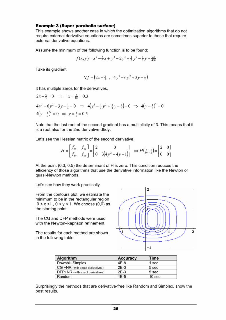
Example 3 (Super parabolic surface) This example shows another case in which the optimization algorithms that do not require external derivative equations are sometimes superior to those that require external derivative equations. Assume the minimum of the following function is to be found:

40061

212

2334

532 2),( +−+−+−= yyyyxxyxf

Take its gradient

( )2123

53 364 , 2 −+−−=∇ yyyxf

It has multiple zeros for the derivatives.

3.0 02 103

53 ==⇒=− xx

( ) ( ) 04 04 0364 321

81

432

233

2123 =−⇒=−+−⇒=−+− yyyyyyy

( ) 5.0 04 213

21 ==⇒=− yy

Note that the last root of the second gradient has a multiplicity of 3. This means that it is a root also for the 2nd derivative df/dy. Let's see the Hessian matrix of the second derivative.

( ) ( )

=⇒

+−

=

=

0002

, 14430

0221

103

2 Hyyff

ffH

yyyx

xyxx

At the point (0.3, 0.5) the determinant of H is zero. This condition reduces the efficiency of those algorithms that use the derivative information like the Newton or quasi-Newton methods. Let's see how they work practically From the contours plot, we estimate the minimum to be in the rectangular region 0 < x <1 , 0 < y < 1. We choose (0,0) as the starting point The CG and DFP methods were used with the Newton-Raphson refinement. The results for each method are shown in the following table.

Algorithm Accuracy Time Downhill-Simplex 4E-8 1 sec CG +NR (with exact derivatives) 2E-3 5 sec DFP+NR (with exact derivatives) 2E-3 5 sec Random 1E-5 10 sec

Surprisingly the methods that are derivative-free like Random and Simplex, show the best results.

27

This happens because they are not affected by the cancellation of the 2nd derivatives On the contrary the other method, also with NR refinement step, cannot reduce the error less then 1E-3. Note that the bigger error happens over the y variable. This is not strange because, as we have demonstrated, the y variable annihilates its 2nd derivatives at the point y = 0.5. Example 4 (The trap) This interesting example shows how to avoid a situation that would trap the most sophisticated algorithms. This happens when there are one or more local extremes near the true absolute minimum. Assume the minimum of the following function is to be found:

( ) ( )22210 2222

5.01),( +−−+−+− −⋅−= yxyxyx eeyxf The contours-plot shows the presence of two extreme points: one in the center (0, 0), called A, and another one in a more narrow region near the point (1, 1), called B

It's interesting to also draw the 3D plot. We note the presence of the larger local minimum at the center point A (0, 0) and the true narrow minimum near the point B. If we choose a starting point like (-1,-1) the algorithm path would likely cross into the point (0, 0) region and will be trapped at this local minimum. On the contrary, if we start from the point (2, 2) it is reasonable to guess that we would find the true minimum. But what will happen if we start from a point like (0, 1) ? Let's see. We try to find the minimum with all the methods, starting from the point (0, 1), in the domains of -2 < x < 2 and -2 < y < 2.

Algorithm x y Accuracy Time

28

Downhill-Simplex 8.38E-08 2.04E-08 - 2 sec

CG 4.03E-08 4.06E-08 - 5 sec

DFP 4.23E-08 4.22E-08 - 6 sec

Random 0.993075 0.993094 1.00E-05 12 sec

As we can see, all algorithms, except one, fail to converge at the true minimum. They all fall into the false central minimum. Only the random algorithm has escaped from the "trap", giving the true minimum with a good accuracy (1E-5). Random algorithms are in general, suitable for finding a narrow global optimum where there are surrounding local optimums.. Convergence region It's reasonable that for the other algorithms there will be some starting points, from which the algorithm will converge to the true minimum B. There will be other starting points that the algorithm will end up at the false minimum (0,0). The set of "good" starting points constitutes the convergence region. A larger convergence region means a robust algorithm. We want to investigate the convergence regions for each of these algorithms. We repeat the above minimum searching with many starting points inside the domain -2 < x < 2 and -2 < y < 2. For each trial we note if the algorithm has failed or not. The results are shown as 2D graphs with the following regions color coded as indicated.

Legend

True minimum False minimum Convergence OK Convergence failed

29

Downhill-Simplex

Conjugate-Gradient and Davidon-Flatcher-Powell

The random algorithm, of course has a convergence region coincident with the black square As we can see, from the point of view of convergence, the most robust algorithm is the Random, followed by the Downhill-Simplex and then by the CG and DFP The Downhill-Simplex has a sufficiently large convergence region and is considered a robust algorithm. The CG, DFP and the NR algorithms have, on the contrary a poor global convergence characteristic. Mixed Method But of course we could use a "mix of algorithms" to reach the best results For example if we start with the random method, we can find a sufficiently accurate starting point for the DFP algorithm. Following this mixed method, we can find the optimum with a very high accuracy (2E-9), no matter what the starting point was.

Algorithm x y Accuracy Time Random+DFP 0.993086 0.993086 1.83E-09 20 sec

30

Example 5 (The eye) Derivative discontinuity in general can give problems to those algorithms using gradient information. But this not always true. Assume the minimum of the following function is to be found:

|1||2| ),( 2 −+−= yxyxf The contour-plot takes on an "eye" pattern for the individual contours. The plot shows that the minimum is clearly the point (2, 1). Note from the 3D plot that the gradient in the minimum is not continuous.

Let's see how the algorithms works, in the domain box 0 < x < 4 and 0 < y < 2 , starting from the point (0, 0)

Algorithm x y error Simplex 2 1 2.34E-13 CG 2.007159289 1 3.58E-03 DFP 2 1 0.00E+00 Random 1.99990227 0.999999965 4.89E-05

A good result. Only the CG algorithm has had some difficulty, but the other algorithms have worked fine. Example 6 (Four Hill) Many times the function to be optimized is symmetric to one or both axes. Assume the maximum of the following function is to be found:

3221),( 2244 +−−+

=yxyx

yxf

Both variables appear only with even powers. So the function is symmetric to both x and y axes. This means that if the function has a maximum in the 1st region {x, y | x>0 , y>0 }, it will have also three other maximum extremes in all other regions. The optimization macros cannot give in one pass, all four maximum points (within the designated region) so one of them is chosen randomly. To avoid this little indecision we must give the initial starting point nearer one of these points or, resizing the convergence region. No too clear? Never mind. Let's see the following plot in the symmetric region

−2 < x < 2 , −2 < y < 2

31

Contours plot

3D plot

It's clear that the function has four symmetric maximums in every region of the selected interval. We can restrict our study to the 1st region 0 < x < 2 , 0 < y < 2. In this region, starting from a point like (2, 2) all algorithms work fine in reaching the true maximum extreme (1, 1) with good accuracy.

Algorithm x y error Simplex 0.999999993 1.000000045 2.59E-08 CG 1.000000005 1.000000005 5.27E-09 DFP 1.000000005 1.000000005 5.27E-09 Random 1.000020331 0.999983443 1.84E-05

More accurate values can be obtained only with the aid of the gradient and the Newton-Raphson extra-step.

( )( )

( )( )

+−−+

−

+−−+

−=∇ 22244

2

22244

2

32214,

32214

yxyxyy

yxyxxxf

Example 7 (Rosenbrock's parabolic valley) This family of test functions is well know to be a minimization problem of high difficulty.

( ) ( )222 1),( xxymyxf −+−⋅= The parameter "m" changes the level of difficulty. A high m value means high difficulty in searching for a minimum. The reason is that the minimum is located in a large flat region with a very low slope. The following plots are obtained for m = 10 Rosenbrock's parabolic valley for m = 10

32

The function is always positive except at the point (1, 1) where it's 0. Taking the gradient it's simple to demonstrate this.

( )( )

=−

=−⋅−+⋅⇒=∇

02022124

02

3

xymymxxm

f

From the second equation, we get:

( ) 22 02 xyxym =⇒=− Substituting in the first equation, we have:

( ) 1 022 022124 23 =⇒=−⇒=−⋅−+⋅ xxxmxxm So the only extreme is at the point (1, 1), which is the absolute minimum of the function. Starting from the point (0, 0) we obtain the following results

Algorithm x y error time Simplex 1 1 2.16E-13 2 sec CG 0.999651904 0.999345232 5.01E-04 50 sec DFP 1.000000003 1.000000005 4.43E-09 55 sec Random 0.999964535 1.000057478 4.65E-05 25 sec

Note that some algorithms may reach the limit in the number of iterations in this example. If we repeat the test with m = 100, we have the following result:

Algorithm x y error time Simplex 1 1 4.19E-13 2 sec CG 0.63263162 0.39851848 4.84E-01 50 sec DFP 0.999906486 0.999732595 1.80E-04 55 sec Random 0.983902616 0.976456954 1.98E-02 25 sec

We note a general loss of accuracy, because all algorithms seem to have difficulty in locating the exact minimum. They seem to get "stuck in the mud" of the valley. Also the random algorithm seems to have a greater difficulty in finding the minimum. The

33

reason is that, when the random algorithm samples a quasi-flat area, all points have similar heights so it has difficulty in discovering where the true minimum is located. The only exception is the Downhill-Simplex algorithm. Its path, rolling into the valley, is both fast and accurate. Why? I have to admit that we cannot explain it... but it works! Rosenbrock's parabolic valley for m = 100

Example 8 (Nonlinear Regression with Absolute Sums) This example explains how to perform a nonlinear regression with objective function different from the Least Squared. In this example we adopt the Absolutes Sum We choose the exponential model:

xkeakaxf ⋅−⋅=),,( The goal of the regression is to find the best couple of parameters values (a, k) that minimize the sum of the absolute value of the difference between the regression model and the given data set.

∑ −= |),,(| kaxfyAS ii The objective function AS depends only on the parameters a and k. By minimizing AS, with our optimization algorithms, we hope to solve the regression problem. A possible arrangement of the worksheet may be:

34

We hope that by changing parameters "a" and "k" in the cells E3 and F3, the objective function in G3 goes to its minimum value. Note that the objective cell G3, being the sum of the range D3:D13, depends indirectly on the cells E3 and F3. Start the Downhill-Simplex and insert the appropriate range as shown in the input box.

Starting from the point (1, 0) you will see the cells changing quickly until the macro stops itself, leaving the following "best" fitting parameter values of the regression y* Best fitting parameters

a k 1 -2

The plot of the y* function and the samples of data set y are shown in the right graph. As we can see the regression fits perfectly the dataset.

35

Example 9 (The ground fault) Assume the minimum of the following function is to be found:

22 )3(11

)1(112),(

−++−

−−+−=

yxyxyxf

The contours and 3D plots of this function are shown in the following graphs

contours-plot

3D plot

Both plots indicate clearly a narrow minimum near the point (2, 1). Nevertheless this function may create some difficulty because the narrow minimum is hidden at the cross of two long valleys (like a ground fault). In order to increase the difficulty, choose a large domain box:

-10 < x < 10 and -10 < y < 10 and (0, 0) as starting point. The results are in the following table

Algorithm x y error time Simplex 1.999999996 1.000000004 7.93E-09 1 sec Random 1.999870157 1.000341845 4.72E-04 9 sec CG 2.000000021 1.00000002 4.08E-08 11 sec DFP 2.00000001 1.000000028 3.80E-08 13 sec

Example 10 (Brown bad scaled function) This function is often used as a benchmark for testing the scaling ability of algorithms

( ) ( ) ( )22626 21010),( −+−+−= − xyyxyxf This function is always positive and it is zero only at the point (106 , 2 10−6 ). At this point, the abscissa is very high and the ordinate is very low. It is hard to generate good plots of this function. We also have no idea where the extremes are located. This situation, is not very common indeed, but if this happens, the only thing that we can do is to run the Downhill-Simplex algorithm trusting in its intrinsically robustness.

36

Algorithm x y rel. errorSimplex 1000000 2.00E-06 1.61E-13

Fortunately, in this case, the algorithm converges quickly to the exact minimun with a very high accuracy Example 11 (Beale function) Another test function that is very difficult to study:

( )[ ] ( )[ ] ( )[ ]23222 1625.2125.215.1),( yxyxyxyxf −−+−−+−−= It is always positive, being a sum of three square terms. So the minimum, if exists, must be positive or 0. Let's try to draw the 3D (see right) The 3D plot, in the range:

−4 < x < 4, −4 < y < 4

shows an extremely flat valley, bordered at the corners with high walls. This plot is quite useless for locating the minimum Let's try with the contours-plot. Maybe we will get some more information.

Contours-plot of the Beale function The plot locates the minimum in the region 0 < x < 5 and 0 < y < 1 We could use (2, 0). as starting point With this initial condition all algorithms work fine.

Algorithm x y error Simplex 3 0.5 3.4E-13 Random 3.000097478 0.5000228382 1.56E-04 CG 3 0.5000000001 1.45E-10 DFP 3 0.5 9.7E-14

Note that the convergence is highly influenced by the starting point. We can verify it simply by starting the CG algorithm from the point (0, 0). The result, after two steps, will be

37

Algorithm x y error iteration CG (1st step) 2.933979062 0.482383744 0.083637 2020 CG (2nd step) 2.999966486 0.499991634 4.19E-05 810

As we can see, the final accuracy is a thousand times less then the previous one. Clearly the time spent for choosing a suitable starting point is useful (This is in general true, when it's possible). Examples of multivariate functions The searching of extremes of a multivariable function, apart from elementary examples, can be very difficult, This is because, in general, we cannot use the graphic method illustrated in the previous examples with one and two variable functions. Sometimes graphic methods may still be applied for particular kinds of functions. Example 1 (Splitting function method) Sometime the function can be split into parts, each having a separate set of variables. If each part contains no more than two variables, we can apply the graphic method for each part.. This example explain this concept. Assume the maximum and the minimum of the following function is to be found:

zxyxzyxzyxf ++⋅+++= 21

23

||||24),,( 22

First of all, we observe that the function has no maximum; so it could have only the minimum. This function can be split into two new functions. One of 2 variables (g(x,y)) and the other of 1 variable h(z).

( ) ( )zzxyxyxzhyxgzyxf +++⋅+=+= 23

21

||2||4)(),(),,( 22

We can plot and study each sub-function separately Contours of g(x,y)

Plot of h(z)

From the first contours-plot we deduce that the minimum is located in the region of −2 < x < 0 and −1 < y < 1. From the second plot we have the region −0.2 < z < 0. Now we have a constraints box for searching for the minimum of f(x,y,z).

38

Let's begin the search with the aid of the random macro. The approximate values obtained by this algorithm will be used for the starting point of all other macros For clarity we have rounded (by it’s not necessary) the values obtained by the random macro give the following approximate starting point

x y z -0.6 0.02 -0.1

The final result is:

Algorithm x y z error time Simplex -0.673971092 0.121063763 -0.111111097 1.10E-08 1 sec CG -0.673969032 0.121061596 -0.11107768 1.83E-05 8 sec DFP -0.673971099 0.12106377 -0.111111112 1.74E-09 10 sec Random -0.674388891 0.019641604 -0.113652504 2.68E-02 5 sec

Example 2 (The gradient condition) Assume the maximum and the minimum of the following function is to be found:

( ) ( ) 22),,( zxyyzxzyxf +−+−= This function is top-unlimited being

+∞===∞→∞→∞→fff

zyxlimlimlim

So we have to study the minimum (if any). The gradient condition is:

=−=−

=−−⇒=∇⇒

−−

−−=∇

02402

022 0

242

22

xzxy

zyxf

xzxy

zyxf

We see that the only point for the minimum is (0, 0, 0). Starting from any point around the origin, every algorithm will converge to the origin.

39

An example of a variation of this function We have seen that this function has no upper limit. This is true if the variables are unconstrained. But surely the maximum exists if the variables are limited by a specific range. Assume now that each variable must be limited in the range [−2, 2]. In this way the maximum surely will belong to the surface of the square box centered around the origin and having length of 4. But where in this box will the maximum be located? It may lie on a face, or on edge, or even at a corner of the box. Let's discover it We can restart the macro "random" searching for the max in the given box or we can also use the CG macro starting from any internal point like for example (1, 1, 1) Here are the results

Algorithm f x y z Random 30.378 -2.057 2.148 2.073 CG 28 -2 2 2

We see that the max, f = 28, is located in the corner (−2, 2, 2) We have to observe that the function is symmetric with respect to the origin.

),,(),,( zyxfzyxf −−−= So there must be another maximum point at the symmetrical point (2, −2, −2). To test for it, simply restart the CG macro, this time choosing the starting point (2, −1, −1). It will converge exactly to the second maximum point. Example 3 (Production) This example shows how to tune the production of several products to maximize profit. The function model here is the Cobb-Douglas production function for three products.

3.03

2.02

1.01 xxxp ⋅⋅=

Where x1, x2, x3 are the quantities of each product (input) and "p" an arbitrary unit-less measure of value of the ouput products. The production cost function can be expressed as

0332211 cxcxcxcc +++= where c1, c2, c3 are the production costs of each item and c0 is a fixed cost. The total profit (our objective function) can then be expressed as g = s·p - c , where s converts the Cobb-Douglas production function "p" value to the same units of cost.

Now let's find the best solution in the Excel worksheet given the following constant values

c1 c2 c3 c0 s 0.3 0.1 0.2 2 2

with the constraints x i > 0 , and with the following maximum limits:

max x1 max x2 max x3 10 50 50

40

A possible arrangement could be

The cost for each item plus the fixed cost and the sale cost factor are in the upper area (grey) The independent quantity and the production quantity are in the middle Finally the quantity constraints are in the bottom area The objective function is in E10 (yellow area)

For a starting point we can use the middle point of each range (5, 25, 25) We then try several algorithms, obtaining the following results

Algorithm x1 x2 x3 rel. error Simplex 2.7463564 16.478137 12.358603 4.92E-08

CG2 2.7463607 16.478145 12.358610 1.77E-06 DFP 2.7463601 16.478219 12.358624 1.01E-05 Random 2.7465324 16.478903 12.359436 1.69E-04

Example 4 (Paraboloid 3D) This is a classical but also a very common surface test

621464265102),( 222 +−−−+−+++= zyxyzxzxyzyxyxf Finding the extremes is easy by solving the following linear system of gradients.

=−++−=−++

=−−+⇒=

⇒=∇021042

014420606264

0 0zyxzyxzyx

fff

f

z

y

x

The solution is (1.4, 0.2, 0.4) Let's see how the algorithms work with this function. Assume a starting point of (0, 0, 0) and a large constraint box:

−10 < x < 10 , −10 < y < 10 and −10 < z < 10

Algorithm x y z error time Simplex 1.400000002 0.199999985 0.400000006 7.89E-09 3 sec Random 1.391827903 0.207765553 0.395835393 6.70E-03 20 sec CG 1.400000021 0.200000017 0.400000008 1.53E-08 8 sec DFP 1.399999897 0.200000048 0.39999996 6.38E-08 4 sec CG+NR 1.4 0.2 0.4 1.00E-16 12 sec DFP+NR 1.4 0.2 0.4 1.00E-16 6 sec

2 the CG algorithm was restarted 2 consecutive times

41

LP - Linear programming A Linear program represent a problem in which we have to find the optima value (maximum or minimum) of a linear function of certain variables (objective function) subject to linear constraints on them. LP - Linear programming This macro solves a linear programming problem by the Simplex algorithm Its input parameters are:

• The coefficients vector of the linear objective function to optimize • The coefficients matrix of the linear constraints

The constraints x i ≥ 0 are implicit. The constraint symbols accepted are "<", ">", "=" "<=", ">=" Let's see how it works with a simple example. Find the maximum of the function

4321 5.03 xxxxF −++= with the following constraints

=+++≥+−

≤−≤+

95.02

072102

4321

432

41

31

xxxxxxx

xxxx

and with

0 , 0 , 0 , 0 4321 ≥≥≥≥ xxxx The following worksheet shows a possible simple arrangement

The range B2:E2 contains the coefficients of the linear objective function The range B4:G7 contains the coefficients matrix of the linear constraints Note: the symbols "<" and "<=" or ">" and ">=" are numerically equivalent for this macro. Now select the objective function range B2:E2 and start the macro Linear Programming from the menu Optimiz... > Optimization Check the input box and click "Run"

42

The solution found, in the range B9:E9 is

x1 = 0 , x2 = 3.375 , x3 = 4.725 , x4 = 0.95 The macro returns "inf" if the feasible region is unbounded; returns "?" if the feasible region is bounded but no solution exist. Observe that this macro does not work on site, therefore it is very fast and can solve more large problems. Example. Find the solution of the following LP problem

{ }54321 42max xxxxx +−+− The matrix constraints is

75 -88 -93 -21 132 ≤ 205-137 -115 75 111 -49 ≤ 146

64 -6 107 -161 -8 ≤ 204-91 -124 -86 154 -74 ≤ 81

-153 -97 9 -152 -79 ≤ -162-135 165 67 185 220 ≤ 1164

90 22 5 138 -111 ≤ 34520 -40 107 -12 -162 ≤ 113

-97 -88 147 86 31 ≤ 31459 -3 142 55 -116 ≤ 335

A possible worksheet arrangement is the following

The solution found by the Simplex algotihm is

x1 x2 x3 x4 x5 3.011 1.539 3.235 1.852 3.442

Note that the value of the function, calculated in the cell L9, is about f ≅ 19.9

43

Optimization with Linear Constraints The Linear Programming seen in the previous chapter is the mostly commonly applied form of constrained optimization. Constrained optimization is much difficult then unconstrained optimization: we have to find the best point of the function respecting all the constraints that may be equalities or inequalities. The solution (the optimum point), in fact, may not occur at the top of a peak or at the bottom of a valley. The main elements of any constrained optimization problem are: the objective function, the variables, the constraints and sometime the variable bounds. When the objective function is not linear (example a quadratic function) and the constraints are linear we have a so called NLP with linear constraints. NLP with linear constraints This macro solves a non-linear programming problem having linear constraints It uses the CG+MC algorithm. This algorithm works fine with quadratic functions but it can also work with other non linear smooth functions It needs information about

1. The cell containing the the function to optimize (objective function)

2. The range of the cells containing the variables to be changed (max 9 variables)

3. The range containing the variable bounds (minimum and maximum limits)

4. The range containing the linear constraints coefficients . The constraint accepted are "<", ">", "<=", ">=" Note that, for this macro, the symbols "<" and "<=" or ">" and ">=" are equivalent. Example: Find the minimum of the function

9822),( 22 +−−+= yxyxyxF with the following constraints

≤≤≤≤

3020

yx

and

≤−≤+12

623yxyx

The following graph shows the contour lines (blue) of the function F(x, y) and the linear constraints (red).

We observe that the "free" minimum of the function is located outside of the feasible region. The constraint minimum lies on the line 3x+2y = 6 .

Now let's see how to compute numerically the constrained optimum point The following worksheet shows a possible arrangement The cell D2 contains the function definition =B2^2+2*C2^2-2*B2-8*C2+9

44

The range B4:C5 is the constraints box and the range B7:E8 contains the two linear constraints.

Note: symbols "<=" and "<" are equivalent for this macro Select the cell D2 and start the macro Linear Constraints from the menu Optimiz... > Optimization

Because this macro works "on site", the solution appears directly in the variables cells B2:C2.

x = 0.727272727272713, y = 1.90909090909093

Compare with the exact solution (8/11, 21/11) Other settings Maximum or Minimum Selection: The two buttons in the upper right of the menu box switch between the minimization and maximization algorithms Stopping Limit. In each panel there is always an input box for setting the maximum number of iterations or the maximum number of evaluation points allowed. The macro stops itself when this limit has been reached. Relative Error Limit: input box for setting the relative error limit. Rnd: this check-box activates/deactivates the random starting algorithm. If selected, the starting point is chosen randomly inside the given constraints box. Otherwise the algorithm starts with the initial variables value (cell B2:C2 of the example). This feature may be useful when we already know a sufficiently close solution or when there are many local optima points. Example: Find the minimum and the maximum of the function

45

11),( 22 +−−−+

=yxxyyx

yxF

with the following constraints

≤≤≤≤

2030

yx

and

−≥−≤−

12

yxyx

The following graph shows the contour lines (blue) of the function F(x, y) , the linear constraints (red) and the box constraints (green).

We observe that the "free" maximum of the function is located inside of the feasible region. The constraint minimum is locate at the corner between the line x-y = 2 and x = 3

Arrange a worksheet as the following inserting the function definition in the cell D3 =1/(B3^2 -B3*C3 -B3 +C3^2 -C3 +2)

If you select the "max" option the algorithm will find the point (1, 1) while if you select the "min" option the algorithm will approach to the point (3, 2) Observe that if you have selected the "Rnd" option, the starting point (0, 0) will be ignored by the macro. On the contrary if you deselect it, you must provide an adapt initial point. In this case we will see that the point (0,0) may be good for the finding the maximum point but with (0, 0) the algorithm fails to reach the minimum point. For the minimum searching we should start, for example, from the point (2, 1)

46

Nonlinear Regression Nonlinear Regression Nonlinear regression is a general fitting procedure that will estimate any kind of relationship between a dependent (or response variable), and a set of independent variables. In this document we focus our attention on unvariate relationships (one response variable "y", one independent variable "x")

)...,,( 21 npppxfy = Where the parameters p1, p2, ...pn are the unknowns to be determined for the best fit. When we investigate the relationship between two variables, we have some steps to follow:

1) Sampling. We take experimental observations of the system in order to get a dataset of n samples (xi, yi) , i =1, ...n. The dimension n varies from few points to thousand of samples.

2) Modelling. At the second step we have to choose a function that should best explain the response variable of the system.

a. This task is dependent on the theoretical aspects of the problem, prior information on the source of the data, what the resulting function will be used for, your imagination or your experience.

b. It would be useful to first plot the points of the dataset in a scatter x-y graph. By a simple inspection we can "smell" which model could be a fit.

c. We have to recognize that the data set has errors of measurement, and that we should not over-fit the model to fit these errors. A knowledge of statistics is important here. We have to recognize that the data is a sample, and that there are sampling errors involved.

d. Actually, we should performs several trials before finally choosing the best model.

3) Prediction. We try to estimate a set of parameter (p1, p2, ...pn)(0) that should approximate the given experimental dataset. These parameter may have some theoretical basis, other than just “fitting” parameters.

4) Starting the fitting process. We try at first with some set of reasonable parameter values as a starting point. We should try several starting points to see if there is a dependency on the results due to different starting points. This is common in scientific problems involving complex functions where the surfaces may have many local minimums, at unknown parameter combinations.

Chapter

3

47

5) Error measurement. Now, by using the fitted model function, we calculate the response values yi* at the same point xi of the sampling. Of course the predicted values will not exactly match the yi values obtained from the sampling, and the differences are the residuals (yi* − yi ). We can take the sum of the square of the residuals RSS = ∑(yi* − yi )2 as a measure of the distance between the experimental data and our model. In other words the RSS measures the goodness of our fit. Low RSS means a more accurate regression fit and vice versa. The error measurement function is also called a loss function.

6) Correction. The initial set of parameter values is changed in order to reduce the RSS function. This is the heart of the non-linear regression process. This task is usually performed with minimization algorithms. We could use any algorithm that we like, but by experience we have observed that some algorithms work better then others. Because the function model is known, and then we also know its derivatives, we could choose an algorithm that exploits the derivative information in order to gain more accuracy.

(a) There is one very efficient algorithm, so called the quasi-Newton, which approximates the second-order derivatives of the loss function to guide the search for the minimum.

(b) The Levenberg-Marquardt is a popular alternative to the Gauss-Newton method of finding the minimum of a function that is a sum of squares of nonlinear functions The Optimiz.xla non-linear fitting process uses just this algorithm for minimizing the residuals squared sum

The set of parameters found at step 5 can now be used for repeating step 3 and, if the process is convergent, after some iterations we'll get the "best" set of parameters (p1, p2, ...pn)(0) . That is the set of parameters best fitting the given dataset, in the sense of the least squared residuals criteria..

48

Nonlinear Regression for general functions Levenberg-Marquardt macro Optmiz.xla has a macro for performing least squares fitting of nonlinear functions directly on the worksheet with the Levenberg-Marquardt algorithm3. It uses the derivatives information (if available) or approximates them internally by the finite difference method. It needs also the function definition cell (=f(x, p1, p2,...), the parameter starting values (p1, p2,...), and of course the dataset (xi, yi). The Levenberg-Marquardt method uses a search direction that is a cross between the Gauss-Newton direction and the steepest descent. It is an heuristic method that works extremely well in practice. It has become a virtual standard for optimization of medium sized nonlinear models.4

The range of (n x m+1) contains the given dataset (x1, x2..xm, y)

Sets the maximun iterations allowed

The range of (n x 1) contains the function definition f(x, a, b, c..) of the regression model

The range of p cells contains the parameters of the regression model. The cells must match the parameters number

The range (n x p) contains the derivatives definition (df/da, df/db, df/dc,...).If empty, the algorithm approximates the derivatives by the finite difference formulas

The check boxes at the right activate/deactivate different elaboration tasks

NLR. Switches on/off the Nonlinear regression

ESD. Calculates the Standard Deviation of the Estimates

RSD. Calculates the Residual Standard Deviation

Layout. In order to automatically fill in the input box, the macro assumes a typical layout: first the x-column, then the y-column at the right, and then the function column. But this is not obligatory at all. You can arrange the sheet as you like Example: Assume that you have the following data set (xi,yi) of 7 observations and you have to perform a least squares fit with the following exponential model having 2 parameters (a, k).

xkeay * ⋅=

3 The Levenberg-Marquardt subroutine used in Optimiz.xla was developed by Luis Isaac Ramos Garcia. Thanks to its kindly contribution we have the chance to publish this nice, efficient -and rare - VB routine in the public domain.

4 The implementation details of how this works are reviewed in Numerical Recipes in C, 2nd Edition, pages 683-685.

49

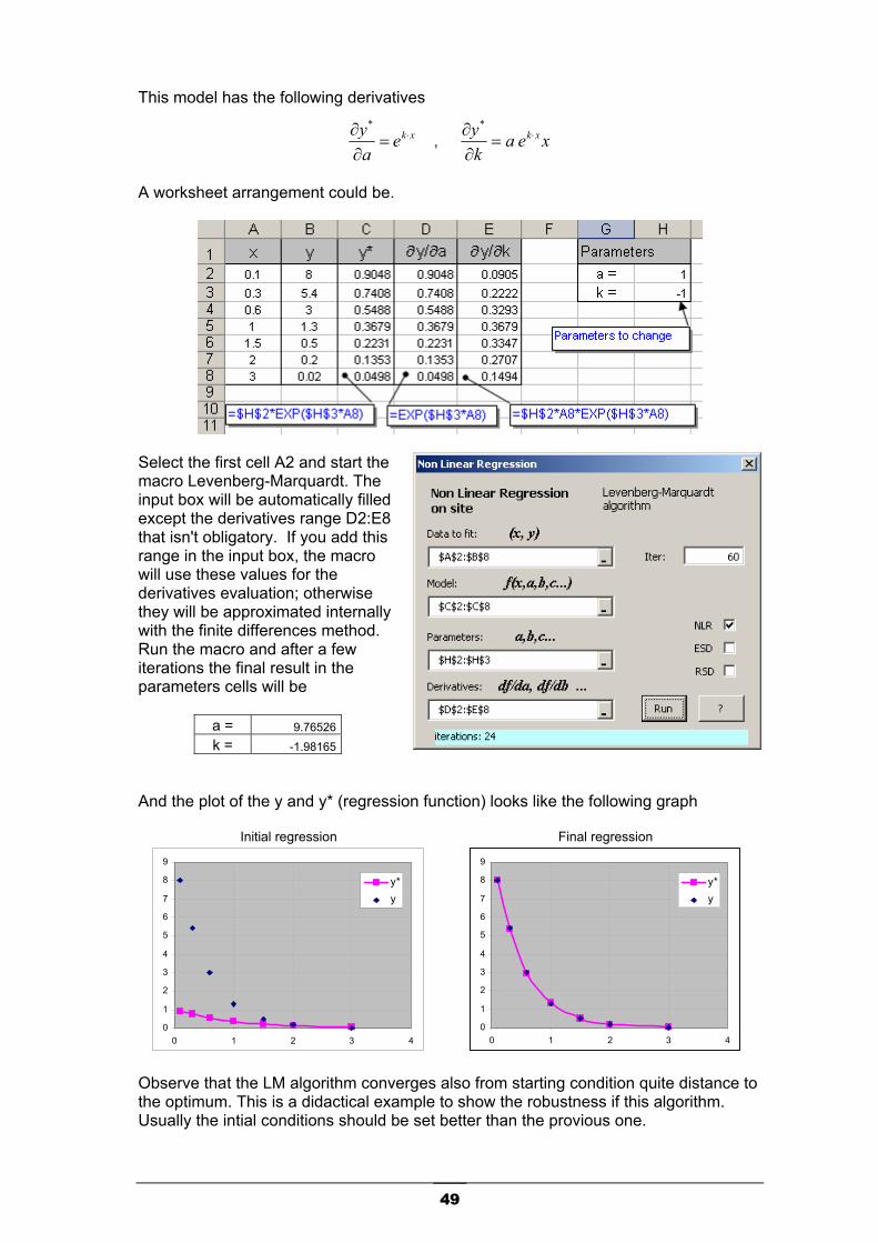
This model has the following derivatives

xkeay ⋅=∂∂

*

, xeaky xk ⋅=∂∂

*

A worksheet arrangement could be.

Select the first cell A2 and start the macro Levenberg-Marquardt. The input box will be automatically filled except the derivatives range D2:E8 that isn't obligatory. If you add this range in the input box, the macro will use these values for the derivatives evaluation; otherwise they will be approximated internally with the finite differences method. Run the macro and after a few iterations the final result in the parameters cells will be

a = 9.76526 k = -1.98165

And the plot of the y and y* (regression function) looks like the following graph

Initial regression Final regression

0

1

2

3

4

5

6

7

8

9

0 1 2 3 4

y*y

0

1

2

3

4

5

6

7

8

9

0 1 2 3 4

y*y

Observe that the LM algorithm converges also from starting condition quite distance to the optimum. This is a didactical example to show the robustness if this algorithm. Usually the intial conditions should be set better than the provious one.

50

Re-try without derivatives. The LM will converge to the same optimal solution. From our experimentation, we have observed that derivatives usually increase the final accuracy of 1-2 order. This macro can manage also multivariable regression. Example. Assume that you have a bidimensional data set (x1, x2, y) and you have to find the best fit with the following rational model having 3 parameters (a, b, c).

2221

21

*

1

xcxxbxay

++=

A worksheet arrangement could be as the following.

The dataset is in the range A2:C12. The cells G2, G3, G4 contains respectively the parameters a, b, c. Each cells of the range C2:C12 contains the model definition. For example the cell D2 contains the formula: =1/($G$2*A2^2+$G$3*A2*B2+$G$4*B2). Choose a compatible starting point - for example a = 1, b = 1, c =1, select the range A2:C12 and start the macro. If you have followed the above disposition all the input box will be correctly filled. Mark the check box "ESD" and "RSD" in order to calculate also the standard deviation of the estimates and the regression. Press "Run"

After a few seconds the macro will converge to the optima solution and will output the standard deviation

The Standard Deviations of the Estimates are always placed adjacent to their parameters. The Residual Standard Error is always output just two rows below the last parameter. So be sure that these cells are empty before starting the macro with the options ESD and RSD active.

51

Nonlinear Regression with a predefined model This set of macros comes in handy when we have to perform a nonlinear regression using a predefined model. They are much faster that the general nonlinear regression macro and, in addition, you do not have to build the formula model and its derivatives. The predefined models added in this version are:

Rational .we can set the degree for numerator and denominator (max degree: 4)

32210

2210

210

10

0

0 , , xxbxbb

xaxaaxxbbxaa

xba

+++++

+++

+

Exponential (from 2 to 6 parameters.)

xkea 1

1⋅ , xkeaa 10

1⋅+ , xkxk eaea 2

1

21 ⋅+⋅ xkxk eaeaa

2

1021 ⋅+⋅+ , xkxkxk eaeaea

3

2

1321 ⋅+⋅+⋅

Damped cosine ( )θω +⋅+ teaa xk cos 10

Power k

k

xaxa , ⋅

Logarithmic bxa +⋅ )log(

Gauss 2

−

−⋅ σ

µx

ea Logistic

xkeababa

)( −+

Input/Output information

All those macros need in input only the data (xi, yi) to fit that must be an array of N rows and 2 columns Output parameters field contains the starting cell where you want to write the unknown parameters. Make sure that the cells below are empty, because the macros will begin to write from the starting cells to the cell below for each parameter to output. Output regression (optional) is the range of cells that you want to fill with the regression values y*. Usually is the column (n x 1) near to the y values column If you check "add formula" the macros will insert the model formula directly into your worksheet instead of the simply

Example

52

The data to fit is the range A2:B8 The output parameter cell is E2. Because the selected model has 3 parameters, the area automatically filled in will be the range E2:F4 The output regression range is C2:C9 Example 1 (Exponential class) To explain how to perform a Nonlinear Least Squares Regression with the aid of Excel and the addin Optimiz.xla we take the example of the standard dataset Misra1a.dat of the NIST/ITL StRD (1978) This dataset contains 14 observations, 1 response variable (y = volume), 1 predictor variable (x = pressure) The model belongs to the "Exponential" class with 2 parameters (b1, b2) to determine y = b1*(1-exp[-b2*x]) Data: y x -------------------------- 10.07E0 77.6E0 14.73E0 114.9E0 17.94E0 141.1E0 23.93E0 190.8E0 29.61E0 239.9E0 35.18E0 289.0E0 40.02E0 332.8E0 44.82E0 378.4E0 50.76E0 434.8E0 55.05E0 477.3E0 61.01E0 536.8E0 66.40E0 593.1E0 75.47E0 689.1E0 81.78E0 760.0E0 We can prepare the worksheet as follows: In the range A2:A15, we insert the x-data. In the next right column B2:B15 the y-data is inserted and in the next column C2:C15, we insert the regression formula, = b1*(1-EXP(−b2*x)) in each cell. The consecutive columns of data x, y and function model y* make up the layout standard for the macro. The parameters b1, b2 are inserted in the cells F5, and F6. For the macro this would be sufficient, but we have inserted other useful functions; (a) calculating the residual squared sum =SUMXMY; (b) computing the relative errors between the certified values and the approximated values =ABS((F6-F10)/F10) , =ABS((F5-F9)/F9); and (c) the Log Relative Error (LRE) = −Log(G5) and = -Log(G6)

NIST-STRD Certified Values b1 = 2.3894212918E+02 b2 = 5.5015643181E-04 Residual Sum of Squares: 1.2455138894E-01

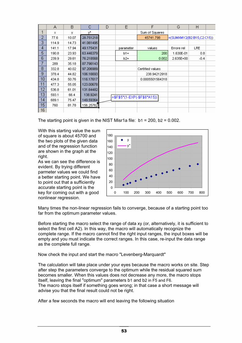
53

The starting point is given in the NIST Misr1a file: b1 = 200, b2 = 0.002. With this starting value the sum of square is about 45700 and the two plots of the given data and of the regression function are shown in the graph at the right. As we can see the difference is evident. By trying different parmeter values we could find a better starting point. We have to point out that a sufficiently accurate starting point is the key for coming out with a good nonlinear regression.

0

20

40

60

80

100

120

140

160

180

0 100 200 300 400 500 600 700 800

y

y*

Many times the non-linear regression fails to converge, because of a starting point too far from the optimum parameter values. Before starting the macro select the range of data xy (or, alternatively, it is sufficient to select the first cell A2). In this way, the macro will automatically recognize the complete range. If the macro cannot find the right input ranges, the input boxes will be empty and you must indicate the correct ranges. In this case, re-input the data range as the complete full range. Now check the input and start the macro "Levenberg-Marquardt" The calculation will take place under your eyes because the macro works on site. Step after step the parameters converge to the optimum while the residual squared sum becomes smaller. When this values does not decrease any more, the macro stops itself, leaving the final "optimum" parameters b1 and b2 in F5 and F6. The macro stops itself if something goes wrong; in that case a short message will advise you that the final result could not be right. After a few seconds the macro will end leaving the following situation

54

0

102030405060708090

0 100 200 300 400 500 600 700 800

y

y*

As we can see the parameters found are different from the certified values by less then 1E-9. The algorithm has caught 8 exact digits out of 10 total digits! Clearly this accuracy is superfluous for a normal fitting, but it is a good example that shows what the Levenberg-Marquardt algorithm can do. We have to point out that sometimes the process cannot give such accurate results. However, by restarting the process with new starting values corresponding to the last set of calculated parameter values, we can see if the values will change to achieve a better fit Remember that your guide for judging a result is always the magnitude of the residuals squared sum (orange cell). Try for example a start with the following parameters b1 = 100, b2= 0.01 (this starting situation is worse that the previous one as you can see from the plot) In this case the macro found new parameters. Even if they seem accurate, these parameter are less accurate then from the previous pass.

parameter values Errore rel LRE b1= 238.94210968 8.161E-08 7.1b2= 0.0005501564842 9.523E-08 7.0

Using this parameters as a new starting point, start again the macro.

parameter values Errore rel LRE b1= 238.94212918 2.934E-12 11.0b2= 0.0005501564318 3.925E-11 10.4

Certified values 238.94212918 0.0005501564318

What happens? The macro has reached the best possible accuracy catching all 10 digits exactly. Clearly this a lucky case but it summarizes a strategy that we should adopt in searching for the best fitting model. Try and.. re-try Example 2 (Exponential Class) Let’s see another example with the standard dataset. Chwirut.dat of the NIST/ITL StRD (197?)) This dataset contains 54 Observations, with one response (y = ultrasonic response) and one predictor (x = metal distance). The model belongs to the "Exponential" class with 3 parameters (b1, b2, b3) and is:

55

xbbey

xb

32

1

+=

−

The dataset is too long to report here, but you can download it from the NIST StRD site. A summary of the NIST certified results are: y = exp(-b1*x)/(b2+b3*x) b1 = 1.6657666537E-01 b2 = 5.1653291286E-03 b3 = 1.2150007096E-02 Residual Sum of Squares: 5.1304802941E+02 Again, in order to choose the starting point, we plot a scatter graph of the dataset. Note that there are multiple y values for a single x. This fact is a very common occurrence with real measurements. We can estimate the exponential dampening factor with the rule of 1/3 decay time. That is: we take the time t* where the y values have decayed to about 1/3 of the initial value. Here the initial value is ymax ≅ 90 and the 1/3 point is about 1.8. From this we estimate b1 = 1/t* ≅ 0.57

0

10

20

30

40

50

60

70

80

90

100

0 1 2 3 4 5 6 7

Another drastic assumption is b1 = 1/100 and b2 = 0. This means that we are beginning with a pure exponential profile, and the starting regression looks like as in the graph (pink-line) The worksheet arrangement could be like the following

Now let's to begin with the regression. Select the cell A2 and start the macro "Levenberg-Marquardt". If you have made the same set-up, you will see the entire input box fill with the correct ranges. Select "Run" and after a few seconds the macro ends leaving the following results

Parameters evaluated certified Rel. error b1 0.16657462110 0.16657666537 1.2272E-05 b2 0.0051652931015 0.0051653291286 6.9748E-06 b3 0.012150093436 0.012150007096 7.1062E-06

res. squared 513.048029438 513.048029410

This is a very accurate result, being that the average relative error is less then 1E-5 and the residual error is close to the expected one.

56

Can we improve the results? Let' see. We restart the algorithm from these values and get a new set of parameter values:

Parameters evaluated certified Rel. error b1 0.16657666491 0.16657666537 2.7602E-09 b2 0.0051653291213 0.0051653291286 1.4206E-09 b3 0.012150007114 0.012150007096 1.4781E-09

As we can see the extra iterations have taken the global relative error to the level of about 1E-9, which is about the minimum that we can get from this data set with the given model. Every other iteration that we could add does not increase the precision any more so we decide to stop the regression. The final result is shown in the right plot. We have to point out that there are other starting points that do not converge to the optimum solution. For example if we start with the parameters: b1 = 1, b2 = 0.01, b3 = 0

0

10

20

30

40

50

60

70

80

90

100

0 1 2 3 4 5 6 7

The result will not converge to the right solution, even if the final fit is not so bad. This is a typical behaviour of the exponential class models

57

Example 3 (using derivatives) This example explains how to use the derivatives with the Levenberg-Marquardt algorithm. This algorithm needs one derivative for each parameter of the model. For example if the model has three parameters, we must provides the information for three partial derivatives:

Model Derivatives

),,,( 321 pppxfy = 321

, , py

py

py

∂∂

∂∂

∂∂

This information is provided indirectly, by an internal subroutine that approximates the derivatives with the finite-difference formula, or directly by writing the derivative formulas into the specific worksheet cells. In this example we performs the regression for the following function model

( ) ( )22

21 arctanarctan xaxay −=

which have the partial derivative

1 ,

1 422

2

242

1

2

1 +−=

∂∂

+=

∂∂

xax

ay

xax

ay

The dataset to fit and its plot is shown below. We have also plot the function (pink-line) having the starting parameters a1 = 0.1 and a2 = 0

x y 0 0

0.1 0.00499970835 0.2 0.01998135315 0.3 0.04478851234 0.4 0.07882527647 0.5 0.12062366858 0.6 0.16746264235 0.7 0.21534838043 0.8 0.25961024656 0.9 0.29599955237

1 0.32175055440 1.1 0.33604846902 1.2 0.33978560977 1.3 0.33490615246

0

0.05

0.1

0.15

0.2

0.25

0.3

0.35

0.4

0 0.2 0.4 0.6 0.8 1 1.2 1.4

In our worksheet, also at the usually information, we have to insert the derivatives functions. A possible arrangement could be the following. The formulas of function and its derivatives must be filled into all cells below the first cell (by dragging)

58

Now we are ready to begin the regression. Let's elect the cell A2 and start the macro. All input boxes will be filled except the derivatives one. Insert the range D2:E15

After few iterations the parameters will converge to the optimum values: a1 = 1 and a2 = 0.5

0

0.05

0.1

0.15

0.2

0.25

0.3

0.35

0.4

0 0.2 0.4 0.6 0.8 1 1.2 1.4

arctan(x2)-arctan(x2 /2)

59

Example 4 (Rational class) The dataset. MGH09.dat from the NIST/ITL StRD (1981) data sets, belongs to the rational equation class of non-linear Least Squares regression. The problem of fitting parameter values was found to be difficult for some very good algorithms. This dataset contains 11 observations, 1 response , 1 predictor and 4 parameters (b1 to b4) to be determined. The equation to be fitted is:

( )43

22

21

bxbxxbxby

+++

=

A summary of the certified NIST results and the data are: y = b1*(x^2+x*b2) / (x^2+x*b3+b4) b1 = 1.9280693458E-01 b2 = 1.9128232873E-01 b3 = 1.2305650693E-01 b4 = 1.3606233068E-01 Residual Sum of Squares: 3.0750560385E-04 Data: y x 1.957000E-01 4.000000E+00 1.947000E-01 2.000000E+00 1.735000E-01 1.000000E+00 1.600000E-01 5.000000E-01 8.440000E-02 2.500000E-01 6.270000E-02 1.670000E-01 4.560000E-02 1.250000E-01 3.420000E-02 1.000000E-01 3.230000E-02 8.330000E-02 2.350000E-02 7.140000E-02 2.460000E-02 6.250000E-02 In order to choose the starting point, we plot a scatter graph of the dataset. We can observe that for x>>1 the intercept is about 0.2, from which we can estimate the parameter b1

2.0lim 1 ≅=∞→

byx We cannot say anything about the other parameters, so they are assumed equal to 1: ( b1= 0.2, b2 = b3 = b4 = 1 ) and the starting function looks like as in the graph (pink-line)

0

0.05

0.1

0.15

0.2

0.25

0 1 2 3 4 5

After 22 iterations we get

Parameter estimated certified rel. error b1 0.19244996595 0.19280693458 1.85E-03 b2 0.19897040739 0.19128232873 4.02E-02 b3 0.12439228242 0.12305650693 1.09E-02 b4 0.13968006879 0.13606233068 2.66E-02

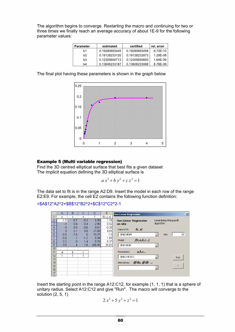
60

The algorithm begins to converge. Restarting the macro and continuing for two or three times we finally reach an average accuracy of about 1E-9 for the following parameter values:

Parameter estimated certified rel. error b1 0.19280693445 0.19280693458 6.73E-10 b2 0.19128233120 0.19128232873 1.29E-08 b3 0.12305650713 0.12305650693 1.64E-09 b4 0.13606233187 0.13606233068 8.78E-09

The final plot having these parameters is shown in the graph below

0

0.05

0.1

0.15

0.2

0.25

0 1 2 3 4 5

Example 5 (Multi variable regression) Find the 3D centred elliptical surface that best fits a given dataset The implicit equation defining the 3D elliptical surface is

1 222 =++ zcybxa The data set to fit is in the range A2:D9. Insert the model in each row of the range E2:E9. For example, the cell E2 contains the following function definition:

=$A$12*A2^2+$B$12*B2^2+$C$12*C2^2-1

Insert the starting point in the range A12:C12, for example (1, 1, 1) that is a sphere of unitary radius. Select A12:C12 and give "Run". The macro will converge to the solution (2, 5, 1)

1 5 2 222 =++ zyx

61

Gaussian regression Gaussian regression is a symmetrical exponential model useful for many applications.

2

−

−⋅= c

bx

eay Three parameters determine completely the Gaussian function a = amplitude b = axis of symmetry c = deviation or spread By inspection of the plot, it is quite easy to recognize and evaluate these parameters:

The axis of symmetry "b" is the abscissa where the function has its maximum amplitude of "a". The deviation "c" is the length where the function is at 37 % of its maximum value. Usually the data are affected by several errors that "mask" the original Gaussian distribution. In that case we can use the regression method to measure how the row data fit the Gaussian model and to evaluate its parameters. Example. Let's see a hypothetical data set (x, y) where the x values of the data are distributed between 98 and 102 The characteristic "bell" distribution is still evident. Near the point x = 100 the distribution has its maximum of about ymax ≅ 1 Deviation is less easy to interpret because of the error, but a rough estimation gives us the value of 0.75

0

0.2

0.4

0.6

0.8

1

1.2

97.5 98 98.5 99 99.5 100 100.5 101 101.5 102 102.5

Now performing the Gauss regression with the Optmiz.xla addin.

62

Select the range of data (x, y) or simply select the first cell A6 of x data and start the macro >Gaussian< of the menu >Non-linear regression< Select the first cell E6 where you want to output the parameters, and press Run

The parameter found will be.

If we plot the Gaussian model with those parameters over the above scattering plot we can observe a good fit.

a = 1.00263 b = 100.0006 c = 0.69677

0

0.2

0.4

0.6

0.8

1

1.2

97.5 98 98.5 99 99.5 100 100.5 101 101.5 102 102.5

63

Rational regression Rational formulas could be used to approximate a wide variety of functions. But the mainly profit happens when we want to interpolate a function near a "pole". Large, sharply oscillations of the system responce could be followed better using a rational model instead other models like polynomials or exponentials. A rational model is a fraction of two polynomials. The max degree of one polynomial gives the degree of the rational model. Usually, in modelling of real stable systems, the denominator degree is always greater then the numerator. The following models have respectively 1, 2 and 3 degree.

xbay+

=0

0

2

10

10

xxbbxaay++

+=

32

210

2210

xxbxbbxaxaay+++

++=

The macro Rational from the menu NL- Regression allows to set separately the numerator and denominator degree. Exanple

In the previous example we have set the numerator degree = 1 and he denominato degree = 2 The macro outputs the coefficients:

Numerator: a0 = 2, a1 = 0 Denominator: b0 = 2, b1 = 0 , b2 = 1 So, the best fitting rational regression model is

222x+

0

0.2

0.4

0.6

0.8

1

1.2

0 1 2 3 4 5

64

When using the rational model The rational model is more complicate then polynomial model. For example a 3 degree rational model has 6 parameters, while the polynomial model of the same degree has 4 parameters. Far from the "pole", the rational model takes no advantage over the polynomial model. Therefore they should be used only when it is truly necessary. The scatter plot of the dataset can helps us in choosing the adapt model. A typical plot that increase or decrease sharply often detects the presence of a "pole" and a 1st degree rational model could be sufficient; on the other hand, if the plot shows a narrow "peak" probably the better choice would be a 2nd degree rational model.

0

1

2

3

4

5

6

7

8

0 0.5 1 1.5 2 2.5 30

0.2

0.4

0.6

0.8

1

1.2

0.5 0.7 0.9 1.1 1.3 1.5

Usually also the inquiry of the system characteristic from witch the samples are given could be help us to choose a suitable rational model degree. Example. The following data was derived from a frequency response of a one-pole system. Find the best fitting model and estimate the pole.

x y 0.5 0.4877814 0.6 0.5978195 0.7 0.4539886 0.8 0.4725799 0.9 0.5267415

1 0.53705 1.1 0.7518795 1.2 0.6314435 1.3 0.8182817 1.4 0.804856 1.5 0.8759378 1.6 1.0459817 1.7 1.1395459 1.8 1.1503947 1.9 1.4471687

2 1.752384 2.1 2.0726757 2.2 2.4904918 2.3 3.3956681 2.4 5.0324014 2.5 10.056427

y = 5.975x4 - 31.287x3 + 57.945x2 - 43.833x + 11.813

0

2

4

6

8

10

12

0 0.5 1 1.5 2 2.5 3

6.21

−−

=x

y

The given data set are interpolated with a 1st degree rational function. The fitting appears good. The pole is the root of the denominator:

x −2.6 = 0 ⇒ x = 2.6

Compare the accuracy and the simplicity of this rational model respect to the one obtained by fitting with a 4th degree polynomial (dotted line)

65

Frequency response of 2nd degree systems often shows a "peak" due to a resonance condition. In this situation rational regression is the only accurate way to fit the data. Compare the regression below obtained with a 2nd degree model (pink line) with the polynomial regression of 6th degree (dotted line) The superiority is evident

-0.2

0

0.2

0.4

0.6

0.8

1

1.2

0.4 0.6 0.8 1 1.2 1.4 1.6

qxxqy

++−=

122

005.0=q

Rational regression gives good results also when same poles is located inside the dataset range. In the following example the dataset is sampled from the function

21)( 2 −

+=xxxf

There is a poles near x = 1.414 but the regression fits very well the same.

-8

-6

-4

-2

0

2

4

6

8

0 1 2 3 4 5

66

Exponential regression Exponential relations are very common in the real world. Usually they appear together with oscillating circular function sine, cosine. In this chapter we investigate the regression of a simple exponential and sum of exponentials. Simple Exponential model The simplest exponential model is

y = A e k x Many books at this point suggest to transform this nonlinear function into a "linearized" one and then apply the linear regression to this new model. The linearization can be made taking the logarithm of sample yi Linearization of the exponential model

ixki eAy ⋅⋅=

Taking the logarithm for each side, we have:

( ) ( ) ( ) ( ) ( ) ( ) ( ) iixk

ixk

i xkAyeAyeAy ii ⋅+=⇒+=⇒⋅= ⋅⋅ loglog logloglog loglog So we obtain the linear function

ii xbbz ⋅+= 10

Where: ( ) ( ) kbAbyz ii === 10 , log , log Performing the linear regression for this model we get the parameters (b0 , b1 ) and finally the original parameter of the nonlinear function (A , k) by these simple formulas

1 , 0 bkeA b ==

This method is quite popular but we have to put in evidence that this method could fail. In fact this is not a true "least squares nonlinear" regression, but a sort of quick method to obtain an approximation of the true "least squares nonlinear" regression. Sometime the parameters obtained by the linearization method are sufficiently close to those of the NL-LS (Non-Linear Least Squares) method; but sometime not and sometime could gives values completely different. So a good technique, always valid to check the result, is to calculate the residuals of the regression. If the least squares of the residual are too high the linearized regression must be rejected. Sometime, the parameters obtained by the linearized method could be used as starting point for the optimization algorithms performing the true NL-LS regression, like the Levenberg-Marqaudt macro of the addin Optimiz.xla Now let' see this example of exponential regression.

x y

0.1 7.9

0.2 7.1

0.3 5.5

0.5 4.1

1 1.3

1.5 0.6

3 0.3

We have to fit the given data point with an exponential model We perform the regression using the linearized method and the NL-LS Exponential method. In Excel we can use the function LOGEST for the first method and use the macro "Exponential Regression" of Optimiz.xla addin for the second method

A possible arrangement in an Excel sheet could be the following

67

the parameter obtained are k1 = −1.1945 a1= 6.9527 giving the following exponential fitting function

xkeay 11=

The column y^ contains the values obtained by the above model

Now perform the regression of the same data with a true NL-exponential regression. Insert the data (x,y) in range A4:B10 and the parameter a1 , k1 in the range F4:F5. Assume the starting point the value given by the above regression k1 = -1.19 a1 = 6.95. Select the range A4:B10 and start the macro "Exponential" of the menu "NL Regression"

Fill the input box with the range F4:F5 and select 2 in the parameters input box. This means that we have chosen the following 2-parameters model

xkeay 11=

We can also choose to output the regression values in the column C4:C10. If we check the "add formula" the macro inserts directly the regression formula into the output cells.

After a while the macro finds the two new optima values a1 = 9.75 , k1 = -1.83 that are quite different form those obtained by the linearized method Now let's to compare the two regressions obtained

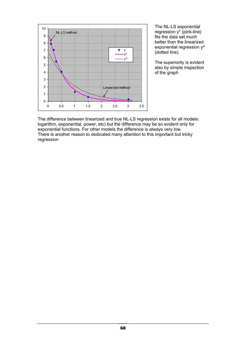
68

The NL-LS exponential regression y* (pink-line) fits the data set much better than the linearized exponential regression y^ (dotted line). The superiority is evident also by simple inspection of the graph

The difference between linearized and true NL-LS regression exists for all models: logarithm, exponential, power, etc) but the difference may be so evident only for exponential functions. For other models the difference is always very low. There is another reason to dedicated many attention to this important but tricky regression

69

Offset Curiously the presence of the simple offset vanish completely the linearization method. When the offset increase respect to the amplitude parameter, the linearized regression becomes much more inaccurate. The only way in this case is the NL-LS regression method with the model

xkeaay ⋅⋅+= 10 Let's see the following example where the data set are generated from the function 10 e-x adding the offset 30 and a bit of random noise

y = 33.043e-0.0213x

29

29.5

30

30.5

31

31.5

32

32.5

33

33.5

34

0 1 2 3 4 5 6

y = 30+10 e-x

The regression function obtained by the linearization method is completely wrong (dotted line). The parameters obtained are k = −0.023 and a = 33 On the contrary the parameters obtained by the true NL exponential regression are: a0 = 30.03, a1 = 10.23, k1 = -1.02, giving a fitting (pink line) much more accettable.

70

Multi-exponentials model The effort for finding a good fitting with a model having two or more exponentials grows sharply. the key of the success is a good starting parameter set. Let's try with the following general two exponential model having 5 parameters

xkxk eaeaay ⋅⋅ ⋅+⋅+= 21210

The scatter plot of the data set (xi,yi) is showed in the dotted line (blue) in the following graph. A reasonable starting point may be taken with the following observation:

0

0.2

0.4

0.6

0.8

1

1.2

1.4

0 1 2 3 4

1) for x >> 0, the curve tends to the value y -> 0.4; therefore we set a0 = 0.4 2) for x = 0, is y(0) = a0 + a1 + a2 . Therefore a2 = y(0) -a0 -a1 Taking a1 = 1 , we get a2 = -1.4 Assume the exponential constants k1 and k2 negative and very different each other: for example take: k1 = -1 , k2 = -10.

With this (rather drastic) assumptions we take the following starting parameters

a0 = 0.4, a1 = 1 , k1 = -1, a2 = -1.4, k2 = -10

which the relative regression function is plotted in the above graph (pink continue line). Start the macro exponential regression, fill correctly the input-box and set the 5th parameters model. We get the final parameters of the exponential regression.

0

0.2

0.4

0.6

0.8

1

1.2

1.4

0 1 2 3 4

a0 = 0.35, a1 = 4.65 , k1 = -1.5,

a2 = -5, k2 = -2.6

71

Good fitting is good regression ? It is the object of the regression to condense and summarize the behaviour of a system by a set of measurements. Usually this is done by a mathematical function- also called "model" - that depends on adjustable parameters. The number of parameters depends by the model complexity; examples of parameters are: growth-rate, concentration, time-decay, pollution, frequency response, etc. When the model parameters are close to the "true" unknown parameters of the system, the experimental data are much close to those extrapolate from the model. This good fitting represents a good agreement between the data and the model. It is also reasonable to think that a good fitting also represent a good estimation of the unknown parameters. It seems reasonable but unfortunately this is not always true, and it happens overall in exponential model. In other words we may have a good fitting without having a good regression model. This means that we could use the model for predicting the values but not for investigating the internal parameter of the system. This simple example shows the concept. Assume to have an electric system that can be modelled with a 2nd order linear-differential equation. This induces us to model its response as a sum of 2 exponentials. Assume to have obtained by three different methods the following three models

xkxk eaeaay ⋅⋅ ⋅+⋅+= 21

210

a0 a1 k1 a2 k2 3 -4 -0.2 10 -1

1.9 -33 -0.66 40 -0.77 0.22 0.25 0.33 8.5 -1.1

At the first sight they are completely different: not only in the exponential amplitudes ( a1 changes from −33 to 0.25 , and a2 from 8.5 to 40) but also in the constant decay factors (k1 changes from −4 to 0.33 becoming positive) But if we plot all these curves we surprisingly observe that they fit each others so good that we cannot distinguee their plots! We can use one of the models to interpolate the points with good accuracy but we could get completely wrong information if we try to make same consideration of the system itself. For example we could predict a potential instability observing the positive exponential of the 3rd model

0123456789

10

0 1 2 3 4 5

On the other hand, if we take good the 1st model, we would believe in a good stability being the damping factor about -1 and -4. But where is the true? As we can see, the consideration about the original system, that is the main goal of the regression, in that case, could be completely wrong.

72

Damped cosine regression That is a very common behaviour of a 2nd order real system. The responce oscillates around a final value with amplitude decreasing with the time.

( )θω ++= teaay t cosk 10

This model has 5 parameters

a0 offset or final value a1 amplitude. k damping factor. ω pulsation (2π f ) θ phase

Related to this model is the following one, called "damped-sine-cosine"

( ) ( )( )tbtbeay scxk sin cos0 ωω ++= ⋅

where : sin , cos 11 θθ abab sc −==

0

0.5

1

1.5

2

2.5

0 0.5 1 1.5 2 2.5 3

The parameters found are: offset 1 amp. 1 damp. -1 puls. 6.283 phase 0

0

0.5

1

1.5

2

2.5

0 0.5 1 1.5 2 2.5 3

Usually the noise mask the original function. In this case we have added 20% of random noise The values found are still very closed to the original parameters and the fitting looks also good: offset 0.997 amp. 1.032 damp. -0.974 puls. 6.259 phase 0.054

73

Power regression The simple model of this regression is

kxay ⋅= with x ≥ 0 and k >0, a >0. When k < 0 the model becames

kxay −=

with x > 0 and a > 0 (x must be strictly positive) Usually this model is used to estimate the growth-rate or decay-rate of a population. We distingue the followinh cases of the exponent parameter k: Case k > 1 The power fitting is very closed to the polynomial fitting when the exponent is positive and greater than 1 ( k > 1) In the right example we can see the polynomial fitting (dotted-line)

y = 0.3 x2 + 0.5 x

and the power function fitting (pink-line)

y = 0.7 x 1.65

They are very closed each others.

y = 0.2992x2 + 0.5118x

0

2

4

6

8

10

12

0 1 2 3 4 5 6

y = 0.7x1.65

Case 0 < k < 1 When the exponent k is positive and lower then 1 , the polynomial model is unsuitable and the power model should be used. In the right example we can see the polynomial fitting (dotted-line)

y = -0.073 x2 + 0.63 x

and the power function fitting (pink-line)

y = 0.7 x 0.45

Only the power function can fit correctly the given data points.

y = -0.0731x2 + 0.6294x

0

0.4

0.8

1.2

1.6

0 1 2 3 4 5 6

y = 0.7 x 0.45

The difficult of the polynomial regression is located near the origin where the derivative grows sharply, becaming infinite for x = 0. Any polynomials, having no singular point, cannot follow the curve near this point. If we would have a dataset far from the singular point x = 0 , also polynomial regression would be better.

74

Case k < 0 When the exponent k is negative the power fitting should be used. Also a logarithmic regression could be used. In the right example we can see the logarithmic fitting (dotted-line)

y = -0.27 log(x) + 0.74

and the power function fitting (pink-line)

y = 0.7 x −0.33

y = -0.2789Ln(x) + 0.7422

0

0.4

0.8

1.2

1.6

0 0.5 1 1.5 2 2.5 3

y = 0.7 x - 0.33

Logarithmic regression Strictly related to the power fitting is the logarithmic regression.

bxay += )log( Where "a" and "b" are parameters to determine. We performs this kind of regression when we have dataset sampled over a wide interval range For example the following dataset cames from the armonic analysis of a system. The vibration amplitude, was measured at 10 different frequencies, from 0.1 KHz to about 2000 KHz We usually plot this dataset with the help of a half-logarithm chart, and thus, it is reasonable to assume also a logarithm regression

x (KHz) y (dB) 0.1 5.334 0.3 3.791 0.9 2.233 2.7 -0.286 8.1 -1.088

24.3 -1.868 72.9 -4.821

218.7 -5.127 656.1 -8.074

1968.3 -10.027 -12

-10-8

-6

-4-2

0

2

46

8

0.1 1 10 100 1000 10000

y = -1.5 Log(x)+2

75

NIST Certification Test The Levenberg-Marquardt macro was recently tested completely with the non-linear NIST StRD dataset. In this test we have used the approximate derivative. For same dataset we have restarted the macro 2 times. When the macro fails the convergence from the 1st starting point, we have started the macro using the 2nd starting point provided by NIST. The test result - the minimum LRE for all regressors - is reported in the following graph, compared with the the Solver of Excel 97

Equation Class NIST Num.

NIST Name

NIST Level

Excel Solver

Optimiz 2.0

Simple Exponential 38 Misrala Lower 4.8 11.1 Simple Exponential 39 Chwirut2 Lower 4.6 10.4 Simple Exponential 40 Chwirut1 Lower 4.9 10.5 Complex Exponentials 41 Lanczos3 Lower 0 8.4 Complex Exponentials 42 Gauss1 Lower 0 10.4 Complex Exponentials 43 Gauss2 Lower 0 9.8 Algebraic 44 DanWood Lower 5.5 11.1 Algebraic 45 Misralb Lower 4.4 12.1 (+) Algebraic 46 Kirby2 Average 1.1 11.4 Algebraic 47 Hahn1 Average 0 9.8 (+) Simple Exponential 48 Nelson Average 1.3 8.7 (*) Simple Exponential 49 MGH17 Average 0 10.2 (*) (+) Complex Exponentials 50 Lanczos1 Average 0 10.6 Complex Exponentials 51 Lanczos2 Average 0 10.0 Complex Exponentials 52 Gauss3 Average 0 10.4 Algebraic 53 Misralc Average 4.6 10.9 Algebraic 54 Misrald Average 5.3 12.5 Trig Function 55 Roszmzn1 Average 3.7 10.0 Algebraic 57 MGH09 Higher 0 9.5 Algebraic 58 Thurber Higher 1.8 9.3 (+) Simple Exponential 59 BoxBOD Higher 0 11.5 (*) Simple Exponential 60 Rat42 Higher 5.3 11.4 Simple Exponential 61 MGH10 Higher 0 9.6 (*) Simple Exponential 62 Eckere4 Higher 0 9.3 (*) Simple Exponential 63 Rat43 Higher 0 9.7 (*) Algebraic 64 Bennett5 Higher 0 8.2

(*) start from 2nd NIST point, (+) 2nd restarting

02468

101214

Mis

rala

Chw

irut2

Chw

irut1

Lanc

zos3

Gau

ss1

Gau

ss2

Dan

Woo

dM

isra

lbKi

rby2

Hah

n1N

elso

nM

GH

17

Lanc

zos1

Lanc

zos2

Gau

ss3

Mis

ralc

Mis

rald

Ros

zmzn

1M

GH

09

Thur

ber

BoxB

OD

Rat

42

MG

H10

Ecke

re4

Rat

43

Benn

ett5

Excel Solver Optimiz

76

Nonlinear Equations Systems Nonlinear Equations Systems Nonlinear Equations Systems Optimiz has a set of macros called rootfinding algorithms concerning the numerical solution of systems of Non-Linear Equations (NLEs).

=

==

0)...,(....

0)...,(0)...,(

21

212

211

nn

n

n

xxxf

xxxfxxxf

0F(x) =⇔

Minimizing versus Rootfinding Strategy We observe that this problem can be reformulated as the minimization of the function

∑=

=n

iin fxxx

1

221 )...,(φ

If we are interested in pursuing this solution strategy, we can adopt all the minimization algorithms contained in this addin but be aware that it is as likely to fail as often as it works, for the following reason. While every root of the system F(x) = 0 is a global minimum of the function φ , there also exist local minima which are not roots of the system. A minimization algorithm is as likely to converge to a local minimum as to a global one, so an abundance these local minima may render such an algorithm practically useless for finding the roots of F(x) . In addition there is another good reason that suggest to use a dedicated rootfinding algorithm for solving the system F(x) = 0; its solution is generally more accurate than the solution obtained by minimization algorithms. On the other hand the minimization algorithms usually shows better convergence performance, therefore, often, the two strategies are used together

Chapter

4

77

NL Equation macros The rootfinding algorithms contained in this addin are: Newton-Raphson This algorithm is the prototype for nearly all NLE solvers. The method works quite well. In the general case, the method converges rapidly (quadratically) towards a solution. The drawbacks of the method are that the Jacobian is expensive to calculate, and there is no guarantee that a root will ever be found unless your starting value is close to the root. This version adopts a relaxation strategy to improve the convergence stability

Working on site.

Broyden This is a so called Quasi-Newton (Variable Metric) method .It avoids the expense of calculating the Jacobian providing a more fast and cheap approximation by generalization of the one-dimensional secant approximation.

Working on site.

Brown The algorithm is based on an iterative method which is a variation of Newton's method using Gaussian elimination in a manner similar to the Gauss-Seidel process. Convergence is roughly quadratic. All partial derivatives required by the algorithm are approximated by first difference quotients. The convergence behavior is affected by the ordering of the equations, and it is advantageous to place linear and mildly nonlinear equations first in the ordering.

Working on site.

Global This macro attempts to find all the solutions in a given range by an hybrid process of 2 algorithms: random sampling and Newton- Maehly method for zeros suppression. Differently from other the macros It does not work on site and It does not need any starting point. It outputs the list of the roots found (if any)

List of roots

1D Rootfinder miscellanea 17 popular algorithms for finding roots of univariate equation

Working on site

78

NLE - Newton-Raphson Solves a system of nonlinear equations using the Newton-Raphson relaxed method Example assume the root of the following system is to be found

=+=⋅⋅−− −

0/10102)840/( 56

yxyyx

In order to locate the root in the plane we use the contour method. The contour plots of the two equations are show in the following graph

The intersection is located in the range: 0 < x < 0.005 and 200 < y < 400

We can arrange the problem in a worksheet. Insert the starting variable values (x0, y0) in the cells B3 and B4 (for example 0, 300) and insert the functions: =B3 -(B4/840)^6 -B4/200000 in the cell E3 and =B3-1/B4 in E4 respectively.

Select the range E3:E4 containing the system to solve and start the macro Newton-Raphson from the menu Optimiz... > NL Equation

If you have followed this procedure the fields will be already filled correctly and you have only to press "run". After few iterations the solution will appear in the cells B3 and B4. Other setting are: Iteration Limit. In the panel there is always an input box for setting the maximum number of iterations allowed. The macro stops itself when this limit has been reached.

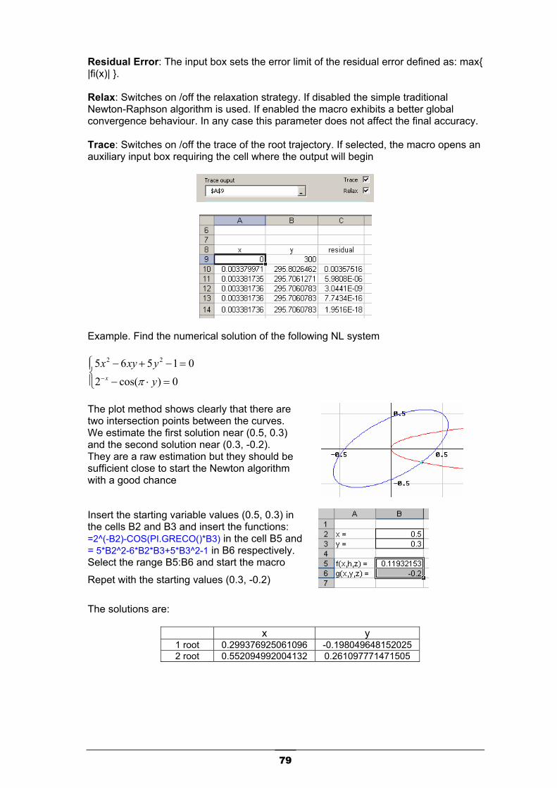
79

Residual Error: The input box sets the error limit of the residual error defined as: max{ |fi(x)| }. Relax: Switches on /off the relaxation strategy. If disabled the simple traditional Newton-Raphson algorithm is used. If enabled the macro exhibits a better global convergence behaviour. In any case this parameter does not affect the final accuracy. Trace: Switches on /off the trace of the root trajectory. If selected, the macro opens an auxiliary input box requiring the cell where the output will begin

Example. Find the numerical solution of the following NL system

=⋅−

=−+−− 0)cos(2

01565 22

yyxyx

x π

The plot method shows clearly that there are two intersection points between the curves. We estimate the first solution near (0.5, 0.3) and the second solution near (0.3, -0.2). They are a raw estimation but they should be sufficient close to start the Newton algorithm with a good chance

Insert the starting variable values (0.5, 0.3) in the cells B2 and B3 and insert the functions: =2^(-B2)-COS(PI.GRECO()*B3) in the cell B5 and = 5*B2^2-6*B2*B3+5*B3^2-1 in B6 respectively. Select the range B5:B6 and start the macro

Repet with the starting values (0.3, -0.2)

The solutions are:

x y 1 root 0.299376925061096 -0.198049648152025 2 root 0.552094992004132 0.261097771471505

80

NLE - Broyden Solves a system of nonlinear equations using the Broyden method Example assume the root of the following system is to be found

=−+

=−+

040162

22

44

yxyx

The contour plots of the two equations are show in the following graph

The 4 intersections are symmetric respect to the origin. One of these is located in the range: 1 < x < 2 and 1 < y < 2

We can arrange the problem in a worksheet. Insert the starting variable values (x0, y0) in the cells A5 and B5 (for example 1, 2) and insert the functions: = A5^4+2*B5^4-16 in the cell C5 and = A5^2+B5^2-4 in D5 respectively. Select the range C5:D5 containing the system to solve and start the macro Broyden from the menu Optimiz... > NL Equation

If you have followed this procedure the fields will be already filled correctly and you have only to press "run". After few iterations the solution will appear in the cells A5 and B5. Other settings

81

Iteration Limit. In the panel there is always an input box for setting the maximum number of iterations allowed. The macro stops itself when this limit has been reached. Residual Error: The input box sets the error limit of the residual error defined as: max{ |fi(x)| }. Trace: Switches on /off the trace of the root trajectory. If selected, the macro opens an auxiliary input box requiring the cell where the output will begin Example. Find the numerical solution of the following NL system

=−+

=−++− 01

012

5.02.1

yexyyx

x

The plot method shows clearly that there are only one intersection point between the curves. We estimate the solution near (0.5, 0.5). It should be sufficient close to start the Broyden algorithm with a good chance.

Insert the starting variable values(0.5, 0.5) in the cells B2 and B3 and insert the functions: = B2*B3+B2^1.2+B3^0.5-1 in the cell B5 and = EXP(-2*B2)+B3-1 in B6 respectively. Select the range B5:B6 and start the macro

The solution is:

x y 1 root 0.283157364898325 0.432386602268468

82

NLE - Brown Solves a system of nonlinear equations using the Brown method Example assume the root of the following system is to be found

=++−−+

=−+−+

0591283033283

223

24

xxxyyxyxyx

The contour plots of the two equations are show in the following graph

There are 4 intersections. One of these is located in the range: 1 < x < 3 and 2 < y < 4 and we may choose the starting point x0= 2, y0 = 4

We can arrange the problem in a worksheet. Insert the starting variable values (x0, y0) in the cells B3 and B4 (for example 1, 4) and insert the functions: = B3^4 + 3*B4^2 - 8*B3 + 2*B4 - 33 in the cell E3 and = B3^3 + 3*B4^2 - 8*B3*B4 - 12*B3^2 + B3 + 59 in E4. Select the range E3:E4 containing the system to solve and start the macro Brown from the menu Optimiz... > NL Equation

If you have followed this procedure the fields will be already filled correctly and you have only to press "run". After few iterations the solution will appear in the cells B3 and B4. Repeating with the starting points (x0,y0) = (3, 0), (x0,y0) = (-2, 0.1), (x0,y0) = (-2, -2) we get all the system solutions

83

Other settings Iteration Limit. In the panel there is always an input box for setting the maximum number of iterations allowed. The macro stops itself when this limit has been reached. Residual Error: The input box sets the error limit of the residual error defined as: max{ |fi(x)| }. Trace: Switches on /off the trace of the root trajectory. If selected, the macro opens an auxiliary input box requiring the cell where the output will begin Example. Find the numerical solution of the following NL system

=−+=−+

012)cos(02)cos(2

yxyx

The plot method shows clearly that there are only one intersection point between the curves. We estimate the solution near (0.5, 0.1). It should be sufficient close to start the Brown algorithm with a good chance.

Insert the starting variable values (0.5. 0.1) in the cells B2 and B3 and insert the functions: = 2*B2+COS(B3)-2 in the cell B5 and = COS(B2)+2*B3-1 in B6 respectively. Select the range B5:B6 and start the macro

The solution is:

x y 1 root 0.5009432689266 0.0614350278365069

84

NLE - Global rootfinder This macro attempts to finds all roots of a nonlinear system in a given space range using the random searching method + the Newton- Maehly formula for zeros suppression. This macro works inside a specific box range and does not need any starting point. It is quite time expensive and, like other rootfinder algorithms, there is no guarantee that the process succeeds. If the macro takes too long try to reduce the searching area. Example assume the root of the following system is to be found

=−++

=−+−

016201

24

22

xyyxxyyx

The contour plots of the two equations are show in the following graph

There are 4 intersections located in the box range

44 ; 44 ≤≤−≤≤− yx

We can arrange the problem in a worksheet. In order to speed up the input filling , this macro assumes the following simple schema:

Insert the functions: = B3^2 - C3^2 + B3*C3 - 1 in the cell D3 = B3^4 + 2*C3^4 + B3*C3 - 16 in E3.

Select the range D3:E3 containing the system to solve and start the macro Global from the menu Optimiz... > NL Equation

85

If you have followed this procedure the fields will be already filled correctly and you have only to press "run" . The macro begins to search for the roots and lists each root found in the cell starting from B8. Because the algorithm proceeds randomly, the roots may appear in any order. The macro stops when it cannot find anymore roots. Other settings Trials. sets the maximum number of random trials allowed for the global searching. For example if the number is 100 (default) then the algorithm samples a random starting point inside the given range at the most for 100 times. This means that, at the most, the macro could find 100 different roots (of course if any trial succeeds) Iteration Limit. sets the maximum number of iterations allowed for each root. When the algorithm overcomes this limit the trial fails and another starting point is sampled. Fails: sets the limit for the stopping criteria. The number 10 (default) means that the macro stops itself when it fails consecutively more than 10% of the total trials. Data Output The macro output the roots and also other interesting data related to each root

err = residual max. error at the current root iter = number of iterations used for finding the current root trial = number of the trial when the current root was found In the above example we see that the the first tow roots were found consecutively at the 1st and 2nd trial, the the algorithm fails the 3rd trial and found the 3rd root at the 4th trial using 24 iterations. After that it fails the trials 5, 6 and 7. Finally it found the last 4th roots at the 8th trial using no more than 7 iterations. Single equation Of course this macro can be used for finding all the root of a single equation Let's see. Find all the roots (if any) of the following equation

04

)cos( =+⋅xxπ

Plotting the equation we note that the roots are located in the range 55 ≤≤− x

86

The number of the roots should be 8, at the least We can arrange the problem in the following way

The function =COS(PI.GREEK()*A3)+1/4*A3 is inserted in the cell D3 Select the cell D4 and start the macro Global

The macro lists 9 roots. The two roots x7 = -4 and x9 = -3.949 are realy very hidden but they can be evidenced by zooming around the point x = 4. As we can see the two distinct roots are confirmed Solving problem "on site", thus directly on the worksheet cells, is more slow then solving by VBA program but, on the other hand, is more flexible because we can use practically all the Excel and user functions that we have. Let's see the following equation Example. Find all the roots of the following equation with the Bessel functions of 1st and 2nd kind

0)4(Y)(J)(Y)4(J 1001 =− xxxx By the graph we observe that the roots are infinite; the first 10 roots are located in the range 100 << x . Note also that the equation is not defined for 0≤x

-0.4

-0.3

-0.2

-0.1

0

0.1

0.2

0.3

0.4

0 1 2 3 4 5 6 7 8 9 10

87

We can arrange the problem in the following way

The function

=BESSEL.J(4*B5;1)*BESSEL.Y(B5;0)-BESSEL.J(B5;0)*BESSEL.Y(4*B5;1)

is inserted in the cell E5. Now select this cell and start the macro Global Set a reasonable number of trial (for example 200) and give "start"

In a few seconds the algorithm has found all the ten roots. Note that the most difficult root to find has been the root 8 = 0.3934562. The algorithm has made 9 trials (24-15 = 9) before finding it. It usually happens when a root is near to same singular point (in that case is x = 0). More variables Solving equations with 3 or more variables may be very difficult because generally we cannot use the graph method. As we have seen it is necessary to locate the space region where the roots are with sufficiently precision. Or, at the least, have an idea of the limits where the variables can move. This is necessary for setting the constraints box. The variable bounding can be often discover by examining the equations of the system itself. Example. Find the solution of the following system

=−++=−++=−++

07.12coscos08.1cos2cos09.1coscos2

zyxzyxzyx

Let's try to find the variable range. For this, we explicit the variable x from the 1st

equation, y from the 2nd and z from the last equation. We have:

88

−−=−−=−−=

2/)coscos7.1(2/)coscos8.1(2/)coscos9.1(

yxzzxyzyx

Because the function cosine is bounded between -1 and 1 the lower and upper bounds for each variable will be

−=−=−=

15.01.005.0

zyx

===

85.19.195.1

zyx

⇒

≤≤−≤≤−≤≤−

313131

zyx

Of course the bounding could be more tight, for example -0.2 ≤ x ≤ 2. But, from our experimentation, the global searching algorithm works better if the constraints box is a bit larger than the one strictly necessary. We can arrange the problem in the following way. Insert in the cells: cell F2 = 2*B2+COS(B3)+COS(B4)-1.9 cell F3 = COS(B2)+2*B3+COS(B4)-1.8 cell F4 = COS(B2)+COS(B3)+2*B4-1.7 The variables x, y, z are the cell B2, B3, B4; the constraints box is inserted in the range C2:D4. Select the range F2:F4 and start the macro Global

In a few second, the macro list the only solution

Variables Solution x -0.0423690502771721 y -0.0941340004413468 z -0.147337615888545

Try to restart several times the macro by the "start" buttom. The algorithm will output the same solution. The same root will also confirmed by other rootfinder algorithms (Newton or Broyden, for example) starting from the point (0, 0, 0) Example. Find the solution of the following system

=−++−

=−+

=+−−

0622

0423

0

22

22

3

xzzxx

zy

yxye x

Let's try to find the variable range. We observe that the equations are "weakly" coupled. That is each equation ties only two variables and, thus, defines an implicit curves that we can plot in order to estimate the limit range of the variables. For convenience we plot the zero contour of the 2nd and 3rd equation

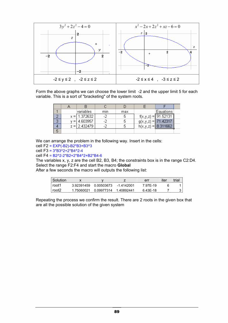
89

0423 22 =−+ zy 0622 22 =−++− xzzxx

-2 ≤ y ≤ 2 , -2 ≤ z ≤ 2 -2 ≤ x ≤ 4 , -3 ≤ z ≤ 2

Form the above graphs we can choose the lower limit -2 and the upper limit 5 for each variable. This is a sort of "bracketing" of the system roots.

We can arrange the problem in the following way. Insert in the cells: cell F2 = EXP(-B2)-B2*B3+B3^3 cell F3 = 3*B3^2+2*B4^2-4 cell F4 = B2^2-2*B2+2*B4^2+B2*B4-6 The variables x, y, z are the cell B2, B3, B4; the constraints box is in the range C2:D4. Select the range F2:F4 and start the macro Global After a few seconds the macro will outputs the following list:

Solution x y z err iter trial root1 3.92391459 0.00503673 -1.4142001 7.97E-19 6 1 root2 1.75060021 0.09977314 1.40892441 6.43E-18 7 3

Repeating the process we confirm the result. There are 2 roots in the given box that are all the possible solution of the given system

90

Univariate Rootfinding macro This macro solves a single nonlinear equation. The user can choose the method among a miscellanea of the most popular rootfinding algorithms. Example. Find the solution of the following equation

01)sin(5.0 =−− xx From the plot we see that the only root lies surely between 0 and 4.

The problem can be arranged as in the following schema. Insert the formula =A3^0.5-SIN(A3)-1 in the cell D3 Select the cell D3 containing the equation to solve and start the macro 1D-Zerofinder misc. from the menu Optimiz... > NL Equation

In this example, we have obtained the numerical solution by the Pegasus algorithm in about 8 iterations with an accuracy better then 1E-15. But we may also try several other algorithms. Other settings Iteration Limit. In the panel there is always an input box for setting the maximum number of iterations allowed. The macro stops itself when this limit has been reached. Residual Error: The input box sets the error limit of the residual error defined as: max{ |fi(x)| }. Trace: Switches on /off the trace of the root trajectory. If selected, the macro opens an auxiliary input box requiring the cell where the output will begin. The first column contains the root value; the second column, the residual error | F(x) |. Algorithm: By this combo-box the user can choose the rootfinding algorithm5 that he like among the following list

5 For further details about these methods see "Nonlinear Equations - Iterative Methods" L. Volpi, 2006, Foxes Team

91

1 "Bisection" Bisection method 2 "Pegasus" Pegasus (Dowell-Jarratt) 3 "Brent" Brent hybrid method (Wijngaardern- Dekker-Brent) 4 "Secant" Secant method 5 "Halley" Halley method 6 "Halley FD" Halley method with finite differences 7 "Secant-back" Secant back-step method 8 "Star E21" Star method (Traub E21) 9 "Parabola" Parabola method

10 "Parabola inv." Inverse parabola method 11 "Fraction" Fraction interpolation method 12 "Newton" Newton-Raphson method 13 "Regula falsi" False position method 14 "Chebychev FD" Chebychev-Householder method with finite differences 15 "Muller" Muller method 16 "Rheinboldt 2" Rheinboldt hybrid method 17 "Steffenson" Steffenson method

Algorithms 5, 12, 17 takes the starting value from the cell "x". The other algorithms start using the points "xmin" and "xmax" of the constraints range. They can be useful for studying and comparing the behavior of several algorithms Example: compare the error trajectories of the Secant, Newton and Halley algorithms applied to the equation

06)3(4 =−+ +−− xee xx

The one-point algorithms "Newton" and "Halley" start from the point inserted in the cell "x" (in that case is 0) The "Secant" algorithm starts using the limits xmin and xmax (in that case 0 and 1) The 2nd column of the each trace is the error |f(x)|. We can compare the trajectories of each algorithm in the following graph.

error trajectories

1E-16

1E-141E-12

1E-10

1E-08

1E-060.0001

0.01

1

1 2 3 4 5 6 7 8 9

SecantNew tonHalley

92

2D - Zero Contour This macro solves the bivariate equation in a plane region x-y

0),( =yxf

As know the solutions form a curve called "zero-contour" or "zero-path" of the function f(x, y). Plotting these curves in a scatter graph we have many useful information about invertibility, intersections with other curves, etc. This macro search for all the points Pi (xi, yi) satisfying the given equation inside a given rectangular region. The points are distant from each other of a given step h in order to form a sort of equispaced path

h

The macro outputs the list of the consecutive points [xi, yi] in two columns A zero contour may be formed by several trees. The macro outputs all the trees separated by an empty row. For example: find the zero-contour of the following equation

1)110(),( 22 −⋅+= yxyxf Because we have no idea where the function has its zeros, we begin with a large searching region and we restrict successively the area in order to have a good positioning of the plot. Here we choose the rectangular range:

11 ; 22 ≤≤−≤≤− yx

Arrange the worksheet like the following and insert the function =(10*B4^2 + 1)^2 *C4^2 - 1 in the cell D4. Then select the cell D4 and start the macro 2D-Zero Path from the menu Optimiz... > NL Equation If you have followed the schema, all the input box will be correctly filled and you have to click "Start" for beginning the path finder. We can also stop the process if it takes too long.

In this case the macro has found a path of by about 200 points in about 7 sec. Observe that each point is an high accurate numerical solution of the equation

0),( =yxf

93

Plotting the data of the range B9:C223 in a scatter x-y graph we get the folloging image

-1

-0.5

0

0.5

1

-2 -1.5 -1 -0.5 0 0.5 1 1.5 2

Note the there are two different trees, simmetrical respect to the x-axis (note also that the range B9:C223 is composed by two separated dataset: the first one in B9:C115 and the second one in B116:C223. They are just the two paths of the zero-contour Other settings Trials. sets the maximum number of random trials allowed. For example if the number is 16 (default) then the algorithm samples a random starting point inside the given range for 16 times. This means that the macro could find at the most 16 different trees of the zero contour. Points: The input box sets the maximum number of the points allowed for all the contour, Increase this value if the contour is very long or has many trees. Step: Sets the space between two consecutive points of the path. Reduce the step only for very detailed paths but remember that the elaboration time will increase sharply. A simple row rule is taking about 1% of the maximum rectangular dimension.

94

Other curves Let's try to plot the zero path of the following equations:

01|||| 3/23/2 =−+ yx

0333 =−+ xyyx

-1

-0.5

0

0.5

1

-1 -0.5 0 0.5 1

-2

-1.5

-1

-0.5

0

0.5

1

1.5

2

-2 -1.5 -1 -0.5 0 0.5 1 1.5 2

02223 =+−+ yxxyx

025166 2224 =+−− yxyxx

-1

-0.5

0

0.5

1

-1 -0.5 0 0.5 1

-1

0

1

2

3

4

5

-5 -4 -3 -2 -1 0 1 2 3 4 5

95

2D Intersection This useful macro extrapolates the intersection between two contours

0),( =yxf , 0),( =yxg

given as two sets of consecutive points (see the macro 2D - Zero Contour)

This algorithm uses the linear interpolation to approximate the intersection. This task may be useful for finding an initial estimation of a nonlinear system solution

==

0),(0),(

yxgyxf

Example: Find a numerical approximation of the solution of the following system

=−++

=−−

0252202222

22

yxyxyx

First of all, we get the zero-contour of each equation by the macro 2D zero contour.

The data set of each path are in the range B10:C167 and D10:E104 respectively. This schema is not obligatory but help in filling the input box of the macro Select the first cell B10 and start the macro 2D Intersection from the menu Optimiz... > NL Equation If you have followed the above schema, all the input box will be correctly filled and you have only to click "Run"

96

The macro has found 4 intersection points

xi yi -0.73892 -0.30292 -0.81216 0.56474 0.73898 0.30312 0.81233 -0.56521

Each value satisfies the given system with an accuracy of about 1E-3 (0.1%), sufficient for graphical representation or as starting point for other, more power, rootfinding algorithms (Newton, Broyden, Brown, etc.)

-2

-1

0

1

2

-2 -1 0 1 2

97

Credits Same of the VB routines contained in this addin was developed with the contribution of the following authors who kindly gave us the permission to release them in the free public domain. Many thanks for this great contributions. "Levenberg-Marquardt nonlinear fitting", "Nelder-Mead Downhill-Simplex" and "linear system routine" have been developed by Luis I. Ramos Garcia. "Broyden nonlinear system solver" has been developed by J.L. Martinez. Many thanks also to D. A. Heiser for his kind contribution in testing, debugging and documentation revision

References Software Sub LMNoLinearFit "Rutina para calcular los valores de ajuste por minimos cuadrados a un modelo Fun(x) mediante el algoritmo de Lebenberg-Marquart", Oct. 2004, by Luis Isaac Ramos Garcia Sub NMSimplex " Rutina para buscar el minimo de una funcion segun el algoritmo de Nelder Mead" Oct. 2004, by Luis Isaac Ramos Garcia Sub SolveLS "Solving Linear System with scaled pivot" Oct. 2004, by Luis Isaac Ramos Garcia and Foxes Team NLE_Broyden "Metodo de Broyden para resolver sistemas de ecuaciones no lineales" by J.L. Martinez and Foxes Team Documents "Numerical Recipes in FORTRAN 77- The Art of Scientific Computing - 1986-1992 by Cambridge University Press. Programs Copyright (C) 1986-1992 by Numerical Recipes Software "Nonlinear regression", Gordon K. Smyth Vol. 3, pp 1405/1411, in Encyclopedia of Environmetrics (ISBN 0471 899976), Edited by John Wiley & Sons, Ltd, Chichester, 2002 "Optimization", Gordon K. Smyth Vol. 3, pp 1481/1487, in Encyclopedia of Environmetrics (ISBN 0471 899976), Edited by John Wiley & Sons, Ltd, Chichester, 2002 "Nonlinear regression", Gordon K. Smyth Vol. 3, pp 1405/1411, in Encyclopedia of Environmetrics (ISBN 0471 899976), Edited by John Wiley & Sons, Ltd, Chichester, 2002 "Process Modeling", The National Institute of Standards and Technology (NIST) website for Statistical Reference Datasets, (http://www.itl.nist.gov/div898/handbook/pmd/pmd) "Metodos Numericos" Sergio R. De Freitas, 2000 "Numerical Mathematics in Scientific Computation", G. Dahlquist, Å. Björck, vol II.

98

"Metodos numericos con Matlab"; J. M Mathewss et al.; Prentice Hall "Numerical Methods that usually work", F. S. Acton, The Mathematica Association of America, 1990 "Analysis Nunerical Methods", E. Isaacson, H. B. Keller, Wiles & Sons, 1966 "Genetic and Nelder-Mead", E. Chelouan, et al, EJOR 148(2003) 335-348 "Convergence properties", J.C. Lagarias, et al, SIAM J Optim. 9(1), 112-147 "The Conjugate Gradient Method", Jim Burke, (http://www.math.washington.edu/ burke) "An Introduction to the Conjugate Gradient Method Without the Agonizing Pain", Jonathan Richard Shewchuk, Edition 114, August 4, 1994, School of Computer Science, Carnegie Mellon University, Pittsburgh "AutoRegression Analysis (AR)", by Paul Bourke, November 1998, (http://astronomy.swin.edu.au/~pbourke/analysis) "Nonlinear Estimation" StatSoft, Inc., 1984-2003 (http://www.statsoftinc.com/textbook/stnonlin) "Optimization for Engineering Systems", Ralph W. Pike, 2001, Louisiana State University (http://www.mpri.lsu.edu/bookindex) "Nonlinear Equations - Iterative Methods" L. Volpi, 2006, Foxes Team (http://digilander.libero.it/foxes) “Advanced Excel for scientific data analysis", Robert de Levie, 2004, Oxford University Press "Microsoft Excel 2000 and 2003 Faults, Problems, Workarounds and Fixes", David A. Heiser, web site http://www.daheiser.info/excel/frontpage.html "NIST/SEMATECH e-Handbook of Statistical Methods", January 26, 2005 (http://www.itl.nist.gov/div898/handbook)

99

WHITE PAGE

100

Analytical Index

A

algorithm; 11

C

CG; 11 Conjugate Gradients; 11 Constraints; 9

D

Davidon-Fletcher-Powell; 11 DFP; 11 Divide-Conquer; 11 Downhill-Simplex; 11

G

Gradient; 8

L

Levenber-Marquaurdt; 12

N

Newton-Raphson; 12 Nonlinear regression; 47

O

Object function; 8

P

Parabolic; 11

R

Random; 11

101

2006, by Foxes Team ITALY

leovlp@libero.it

2. Edition May 2006