optimization in economics and financ ekhuongnguyen.free.fr/ebooks/springer- dynamic modeling...
TRANSCRIPT
OPTIMIZATION IN ECONOMICS AND FINANCE
Dynamic Modeling and Econometrics in Economicsand FinanceVOLUME 7
Series Editors
Stefan Mittnik, University of Kiel, GermanyWilli Semmler, University of Bielefeld, Germany and
New School for Social Research, U.S.A.
The titles published in this series are listed at the end of this volume.
Optimization in Economicsand Finance
Some Advances in Non-Linear, Dynamic,Multi-Criteria and Stochastic Models
by
BRUCE D. CRAVENUniversity of Melbourne, VIC, Australia
and
SARDAR M. N. ISLAMVictoria University, Melbourne, VIC, Australia
A C.I.P. Catalogue record for this book is available from the Library of Congress.
ISBN 0-387-24279-1 (HB)
ISBN 0-387-24280-5 (e-book)
Published by Springer,
P.O. Box 17, 3300 AA Dordrecht, The Netherlands.
Sold and distributed in North, Central and South America
by Springer,
101 Philip Drive, Norwell, MA 02061, U.S.A.
In all other countries, sold and distributed
by Springer,
P.O. Box 322, 3300 AH Dordrecht, The Netherlands.
Printed on acid-free paper
All Rights Reserved
© 2005 Springer
No part of this work may be reproduced, stored in a retrieval system, or transmitted
in any form or by any means, electronic, mechanical, photocopying, microfilming, recording
or otherwise, without written permission from the Publisher, with the exception
of any material supplied specifically for the purpose of being entered
and executed on a computer system, for exclusive use by the purchaser of the work.
Printed in the Netherlands.
v
Table of Contents
Preface ix
Acknowledgements and Sources of Materials xi
Chapter One: Introduction :Optimal Models for Economics and Finance 1
1.1 Introduction 11.2 Welfare economics and social choice: modelling and applications 21.3 The objectives of this book 51.4 An example of an optimal control model 61.5 The structure of the book 7
Chapter Two: Mathematics of Optimal Control 92.1 Optimization and optimal control models 92.2 Outline of the Pontryagin Theory 122.3 When is an optimum reached? 142.4 Relaxing the convex assumptions 162.5 Can there be several optima? 182.6 Jump behaviour with a pseudoconcave objective 202.7 Generalized duality 242.8 Multiobjective (Pareto) optimization 292.9 Multiobjective optimal control 302.10 Multiobjective Pontryagin conditions 32
Chapter Three: Computing Optimal Control:The SCOM package 35
3.1 Formulation and computational approach 353.2 Computational requirements 373.3 Using the SCOM package 403.4 Detailed account of the SCOM package 413.4.1 Preamble 413.4.2 Format of problem 413.4.3 The SCOM codes: The user does not alter them 42
3.5 Functions for the first test problem 463.6 The second test problem 473.7 The third test problem 49
Chapter Four: Computing Optimal Growthand Development Models 55
4.1 Introduction 55

vi
4.2 The Kendrick-Taylor growth model 564.3 The Kendrick-Taylor model implementation 574.4 Mathematical and economic properties of the results 604.5 Computation by other computer programs 644.6 Conclusions 64
Chapter Five: Modelling Financial Investmentwith Growth 66
5.1 Introduction 665.2 Some related literature 665.3 Some approaches 695.4 A proposed model for interaction between investment and physical
capital 705.5 A computed model with small stochastic term 725.6 Multiple steady states in a dynamic financial model 755.7 Sensitivity questions concerning infinite horizons 805.8 Some conclusions 815.9 The MATLAB codes 825.10 The continuity required for stability 83
Chapter Six: Modelling Sustainable Development 846.1 Introduction 846.2 Welfare measures and models for sustainability 846.3 Modelling sustainability 876.3.1 Description by objective function with parameters 876.3.2 Modified discounting for long-term modelling 896.3.3 Infinite horizon model 90
6.4 Approaches that might be computed 926.4.1 Computing for a large time horizon 926.4.2 The Chichilnisky compared with penalty term model 926.4.3 Chichilnisky model compared with penalty model 946.4.4 Pareto optimum and intergenerational equality 956.4.5 Computing with a modified discount factor 95
6.5 Computation of the Kendrick-Taylor model 966.5.1 The Kendrick-Taylor model 966.5.2 Extending the Kendrick-Taylor model to include a long time
horizon 976.5.3 Chichilnisky variant of Kendrick-Taylor model 986.5.4 Transformation of the Kendrick-Taylor model 98
6.6 Computer packages and results of computation of models 996.6.1 Packages used 996.6.2 Results: comparison of the basic model solution with results for
modified discount factor 996.6.3 Results: effect of increasing the horizon T 101

vii
6.6.4 Results: Effect of omitting the growth term in the dynamicequation 103
6.6.5 Results: parametric approach 1036.6.6 Results: the modified Chichilnisky approach 105
6.7 Existence, uniqueness and global optimization 1086.8 Conclusions 1096.9 User programs for transformed Kendrick-Taylor model for
sustainable growth 110
Chapter Seven : Modelling and Computing a StochasticGrowth Model 111
7.1 Introduction 1127.2 Modelling stochastic growth 1127.3 Calculating mean and variance 1137.4 Computed results for stochastic growth 1147.5 Requirements for RIOTS 95 as M-files 116
Chapter Eight: Optimization in Welfare Economics 1238.1 Static and dynamic optimization 1238.2 Some static welfare models 1238.3 Perturbations and stability 1258.4 Some multiobjective optimal control models 1268.5 Computing multiobjective optima 1288.6 Some conditions for invexity 1298.7 Discussion 130
Chapter 9: Transversality Conditions for InfiniteHorizon Models 131
9.1 Introduction 1319.2 Critical literature survey and extensions 1319.3 Standard optimal control model 1359.4. Gradient conditions for transversality 1369.5 The model with infinite horizon 1399.6 Normalizing a growth model with infinite horizon models 1399.7 Shadow prices 1419.8 Sufficiency conditions 1429.9 Computational approaches for infinite horizon 1439.10 Optimal control models in finance: special considerations 1469.11 Conclusions 146
Chapter 10: Conclusions 147
Bibliography 149

viii
Index 158
ix
PrefaceMany optimization questions arise in economics and finance; an important
example of this is the society’s choice of the optimum state of the economy(which we call a social choice problem). This book,
Optimization in Economics and Finance,
extends and improves the usual optimization techniques, in a form that maybe adopted for modelling optimal social choice problems, and other relatedapplicastions discussed in section 1.2, concerning new3 economics. These typesof optimization models, based on welfare economics, are appropriate, since theyallow an explicit incorporation of social value judgments and the characteristicsof the underlying socio-economic organization in economic and finance models,and provide realistic welfare maximizing optimal resource allocation and socialchoices, and decisions consistent with the reality of the economy under study.The methodological questions discussed include:
• when is an optimum reached, and when is it unique?• relaxation of the conventional convex (or concave) assumptions on aneconomic or financial model,• associated mathematical concepts such as invex (relaxing convex) andquasimax (relaxing maximum),• multiobjective optimal control models, and• related computational methods and programs.These techniques are applied to models of economic gropwth and develop-
ment, including• small stochastic perturbations,• finance and financial investment models (and the interaction betweenfinancial and production variables),• modelling sustainability over long time horizons,• boundary (transversality) conditions, and• models with several conflicting objectives.
Although the applications are general and illustrative, the models in thisbook provide examples of possible models for a society’s social choice for anallocation that maximizes welfare and utilization of resources. As well as us-ing existing computer programs for optimization of models, a new computerprogram, named SCOM, is presented in this book for computing social choicemodels by optimal control.
This book contains material both unpuhlished and previously publishedby the authors, now rearranged in a unified framework, to show the relationsbetween the topics and methods, and their applicability to questions of socialchnoice and decision making.
This book provides a rigorous study on the interfaces between mathemat-ics, computer programming, finance and economics. The book is suitable as a
x
reference book for researchers, academics, and doctoral students in the area ofmathematics, finance, and economics.
The models and methods presented in this book will have academic andprofesional application to a wide range of areas in economics, finance, andapplied mathematics, including optimal social choice and policy planning, useof optimal models for forecasting, market simulation, developmenjt planning,and sensitivity analysis.
Since this is an interdisciplinary study involving mathematics, economics,finance and computer programming, readers of this book are expected to havesome familiarity with the following subjects: Mathematical Analysis, OptimalControl, Mathematical Finance, Mathematical Economics, Mathematical Pro-gramming, Growth Economics, Economic Planning, Environmental Economics,Economics of Uncertainty, Welfare Economics, and Computational Economics.
The various SCOM computer programs listed in this book may also bedownloaded from the web site: http://bdc.customer.netspace.net.au .
The authors thank Margarita Kumnick for valuable proof-reading andchecking. The authors also thank the Publishing Editor of Kluwer, Mrs Cathe-lijne van Herwaarden, and a referee, for their cooperation and support in thecompletion of this book.
B. D. Craven S. M. N. Islam 1 September 2004Dept. of Mathematics Centre for Strategic& Statistics Economic StudiesUniversity of Melbourne Victoria University, MelbourneAustralia Australia
The authors
Dr. B. D. Craven was (until retirement) a Reader in Math-ematics at University of Melbourne, Australia, where he taught Mathematicsand various topics in Operations Research for over 35 years. He holds a D.Sc.degree from University of Melbourne. His research interests include continuousoptimization, nonlinear and multiobjective optimization, and optimal controland their applications. He has published five books, including two on mathe-matical programming and optimal control, and many papers in internationaljournals. He is a member of Australian Society for Operations Research andINFORMS.
Prof. Sardar M. N. Islam is Professor of Welfareand Environmental Economics at Victoria University, Australia. He is also as-sociated with the Financial Modelling Program, and the Law and EconomicsProgram there. He has published 11 books and monographs and more than 150technical papers in Economics (Mathematical Economics, Applied Welfare Eco-nomics, Optimal Growth), Corporate Governance, Finance, and E-Commerce.

xi
Acknowledgements and Sources of MaterialsThe authors acknowledge permission given by the following publishers to
reproduce in this book some material based on their published articles andchapters:
Chapter 3 is based (with some additional material) on Computing OptimalControl on MATLAB - The SCOM Package and Economic Growth Models,Chapter 5 in Optimisation and Related Topics, Eds, A. Rubinov et al. Vol-ume 47 in the Series Applied Optimization, Kluwer Academic Publishers, 2001.Kluwer has given permission to reproduce this article.
Chapter 4 is (with minor changes) the paper Computation of Non-LinearContinuous Optimal Growth Models: Experiments with Optimal Control Algo-rithms and Computer Programs, 2001, Economic Modelling: The InternationalJournal of Theoretical and Applied Papers on Economic Modelling, Vol. 18,pp. 551-586, North Holland Publishing Co.
Chapter 6 is (with minor modifications) the paper Measuring Sustain-able Growth and Welfare: Computational Models, Methods, Editors: ThomasFetherston and Jonathan Batten, “Governance and Social Responsibility”,Elsevier-North Holland, 2003.
Chapter 9 is the paper Transversality Conditions for Infinite Horizon Op-timal Control Models in Economics and Finance, submitted to Journal of Eco-nomic Dynamcs and Control, an Elsevier publication.
Elsevier have stated that an Elsevier author retains the right to use anarticle in a printed compilation of works of the authors.
The book also includes excerpts from other papers by the authors, oftenrearranged to show relevance and relation to other topics; these items are ac-knowledged where they occur. The material in this book is now presented ina unified manner, with a focus on applicability to economic issues of socialchoice.

Chapter 1Introduction :
Optimal Models forEconomics and Finance
1.1. IntroductionThis book is concerned with applied quantitative welfare economics, and
describes methods for specification, analysis, optimization and computation foreconomic and financial models, capable of addressing normative social choiceand policy formulation problems. Here social choice refers to the optimal in-tertemporal allocation of aggregate and disaggregate resources. The institu-tional and organizational aspects of achieving such allocation in a society arenot discussed here. Zahedi (2001) has surveyed other methods for social choice.The book aims to provide some extensions and improvements to the traditionalmethods of optimization, as applied to economics and finance, which could beadopted for social decision making (social choice) and related applications.The mathematical techniques include nonlinear programming, optimal control,stochastic modelling, and multicriteria optimization.
Many questions of optimization and optimal control arise in economics andfinance. An optimum (maximum or minimum) is sought for some objectivefunction, subject to constraints (equalities or inequalities) on the values of thevariables. The functions describing the system are often nonlinear. For a time-dependent system, the variables become functions of time, and this leads toan optimal control problem. A control function describes a quantity (such asconsumption, or investment) that can be controlled, within some bounds. Astate function (such as capital accumulation) takes values determined by thecontrol function(s) and the dynamic equation(s) of the system.
Some recent developments in the mathematics of optimization, includingthe concepts of invexity and quasimax, have not previously been applied tomodels of economic growth, and to finance and investment. Their applicationsto these areas are shown in this book. Some results are presented concerningwhen an optimal control model has a unique optimum, what happens whenthe usual convexity assumptions are weakened or absent, and stability to smalldisturbances of the model or its parameters. A new computational packagecalled SCOM, for solving optimal control problems on MATLAB, is introduced.It facilitates computational experiments, in which there are changes to modelfeatures or parameters.
These developments are applied, in particular, to:• models of optimal (welfare maximizing) intertemporal allocation ofresources.
2 Chapter 1
• economic growth models with a small stochastic perturbation.• models for finance and investment, including some stochastic elements,and especially considering the interaction between financial and productionvariables.• modelling sustainability over a long (perhaps infinite) time horizon.• models with several conflicting objectives.• boundary (transversality) conditions.These extended results can be usefully applied to various questions in
economics and finance, including social decision making and policy analysis,forecasting, market simulation, sensitivity analysis, comparative static and dy-namic analysis, planning, mechanism design, and empirical investigations. Ifan economic system behaves so as to optimize some objective, then a computedoptimum of a model may be used for forecasting some way into the future. How-ever, the book is focussed on optimal social decision making (social choice).
1.2. Welfare economics and social choice: Modelling and Applica-tions
A central issue in economics and finance, concerning welfare economics,is to find a normative framework and methodology for social decision-making,so as to choose the socially desirable (multi-agent or even aggregate) state ofthe economy, a task popularly known as ”social choice”. Optimisation methodsbased on welfare economics can aid such social decision making ((Islam 2001a).
The optimisation models of economics and finance can, therefore, be in-terpreted as models for normative social choice which specify optimal socialwelfare in the economy and financial sector satisfying the static and dynamicconstraints of the economy since these models can generate a set of aggregativeand disaggregstive optimal decisions. choices or allocation of resources for thesociety. This approach is in the line of arguments advanced in the paradigmof new3 welfare economics (Islam 2001b; Clarke and Islam, 2004). It has thefollowing main elements: 1) the possibility perspective of social choice theory;2) measurability of social welfare based on subjective or objective measures;3) the extended welfare criteria; 4) operationalisation of welfare economicsand social choice (which was the original motivation of classical economists fordeveloping the discipline of welfare economics), and 5) a multi-disciplinary sys-tem approach incorporating welfaristic and non-welfaristic elements of socialwelfare.
Any welfare economic analysis of issues in economics and financial policiesinvolves the application of the following multidisciplinary criteria of moral phi-losophy and welfare economics: efficiency, rationality, equity, liberty, freedom,capabilities and functioning (see Hausman and McPherson, 1996) for a surveyof these criteria). This framework of new3 welfare economies provides the scopefor evaluating economic outcomes in terms of social welfare (and efficiency, util-ity) as well as other criteria of welfare economics and moral philosophy such asrights, liberty, morality, etc. (see Hausman and McPherson, 1996 for a surveyof the concepts and issues and their economic implications).
Optimal Models Economics Finance 3
The incorporation of this approach in optimisation modelling is possiblethrough the choice of the social discount rate, the objective function (extendedwelfare criteria incorporating welfaristic and non-welfaristic elements of socialwelfare), terminal conditions, time horizon, and the modelling structure.
In making such an application of optimisation models, several conceptualand methodological issues in social choice theory and welfare economics (whichhave dominated the controversy about the possibility of social choice) needs tobe resolved including the following (Islam 2001b):
• The nature value judgment about the nature of individual well-being orwelfare (such as in utilitarianism or welfarism, capability,) etc.• Possibilities for measurability of utility and welfare (cardinality orordinality).• Interpersonal comparability of utility and welfare.• The nature of marginal utility of income (constancy or variability).• The role of distributional concerns in welfare judgment (the intensity ofpreferences).• The choice of a measurement and accounting method (nature ofpreference indexing, numerical calculations, etc.).• The extent of informational requirements for decision making.These issues can be considered from the impossibility (Arrow, 1951) or
possibility perspectives (Sen, 1970). The possibility perspective approach re-quires a set of axioms including cardinality, intertemporal comparability, andthe relevance of the intensity of preferences. In this possibility approach (seeSen 1999), there is an urge for the need for, amongst others, finding a suit-able method and information broadening for developing an optimistic socialchoice theory for useful social welfare analysis and judgment. This can be ac-complished by developing an operational approach to social choice. This isan especially immediate task in applied welfare economics, although work inthis area has not progressed far. In Islam (2001a, 2001b) and Clarke and Is-lam (2004), a paradigm has been developed for new3 welfare economics, fornormative operational social choices based on the possibility perspective.
The choice of the elements for a social norm is controversial, since eachspecification relates to some form of value judgment in a welfare economicschoice model, and a choice significantly affects the pattern and level of socialwelfare. A specification of the the elements of a social choice should be basedwithin the framework of some paradigm of welfare economics. The new3 welfareeconomics paradigm adopts the following set of assumptions and elements ofan operational approach to social choice aqnd decision making:
• Definition of well-being and welfare: the social welfaristic approach(Islam 2001a and 2001b) - economic activities, which improve net socialwelfare, are justified.• The possibility of the specification of aggregate social welfare criteriaand index: the possibility theorem perspective.• Time preference: different discounting approaches for intertemporal
4 Chapter 1
equity - depending on the preference of the society.• Units of measurement; market and shadow prices of goods and services• Methods for modelling: efficient allocation or optimisation modelling.• Institutions: various alternative institutions can be assumed such ascompetitive market economy, mixed economy, or planning - depending onthe underlying social organization.The main argument of this book is that mathematical models can be de-
veloped, incorporating the above elements of new3 welfare economics; they canprovide useful information to understand social choice in relevant economic, so-cial, environmental and financial issues, and formulating appropriate policies.
The general structure of an optimisation model in economics and finance,containing the above elements, and suitable for normative social choice or de-cision making (see Craven 1995; Islam 2001a; Laffont, 1988) is as follows:
W = f(y) subject to g(y) ∈ S,
where: I = [a, b];W is an indicator of social welfare;V is the space of functions;f(y) is a scalar or vector valued social welfare functional of society.y is a vector of variables or functions of economic and financialsub-systems;g(y) is a constraint function (including economic and financialfactors);S is a convex cone, describing a feasible set of the economy; andRn is Euclidian space of n dimensions.In the above social welfare model, a social welfare function of the Bergson-
Samuelson form is specified to embed social welfare judgments about alterna-tive states of resource allocation in the economy. (For further details, see Islam,2001a.) Social welfare, and factors affecting it, are assumed to be measurableand quantifiable. The problem of normative social choice in decision making isrepresented by the optimization model, based on the possibility perspective ofsocial choice. It is operational, since it may be applied to real life conditions,for finding optimal decisions in society. The model can represent the economicorganization of a competitive market or planning system (the selection of asystem of social organization depends on the social preferences assumed in themodel). A model, containing an objective function, constraints and boundaryconditions, can represent the socio-economic factors relevant for decision mak-ing. These general assumptions are made for the various models in this book;specific assumptions for each model are discussed in the relevant cases.
The optimal solution to the welfare optimisation social choice problemexists (i.e., an optimal decision, choice, or policy exits) if the problem satisfiesthe Weierstrass theorem; and if the objective function is convex, x* is a globalsolution.
Optimal Models Economics Finance 5
The set S represents the static or dynamic economic and financial sys-tems. The objective function f(x) is the social welfare functional embeddingsocial choice criteria. Different value judgements and different theories of wel-fare economics and social choice, and various sub-systems of the economy canbe incorporated in this social choice program by making different assumptionsabout different functions, parameters and the structure of the above model.The above control model can embed and address the issues of welfare eco-nomics and social choice discussed above if it is based on a proper specificationof the method for aggregation of individual welfare, welfare criteria, cost benefitconsideration, and institutional mechanisms assumed for society. The resultsof the model can specify the optimal choices regarding optimal dynamic welfareand resource allocation and price structure, the optimal rate and valuation ofconsumption, capital accumulation, and other economic activities, and optimalinstitutional and mechanism design. Further discussion on construction of wel-fare economic modelling is given in Islam (2001a), Heal (1973), Chakravarty(1969), and Fox, Sengupta and Thorbecke (1973).
The above social choice model is a finite horizon free terminal time con-tinuous optimisation problem and it is deterministic, and open loop with socialwelfare maximization criteria. Other possible forms of social choice modelsinclude dynamic game models and with other types of end points and transver-sality conditions; overtaking, catching up and Rawlsian optimality criteria; withdifferent types of constraints, discontinuities and jumps; and with uncertainty.These social choice models may also represent equilibrium and disequilibriumeconomic systems, adaptive dynamics, social learning, chaotic behaviour, arti-ficial intelligence and genetic algorithm.
In such an optimisation model of social choice, the following set of elementsshould be specified:
• an economic model (including social, financial, and environmentalconstraints;• the length of the planning horizon;• the choice of an optimality criterion or an intertemporal utility function;• the discount rate, representing the rate of time preference; and• the terminal or transversality conditions.The specification of the elements is a political economic exercise involving
substantial value judgment on the part of the modeller. Depending on the valuejudgment of the modeller, a particular form of each element can be specified.
1.3. The objectivesThe objective of this book is to provide extensions to the existing methods
for optimisation in economics and finance which can be appropriately used fornormative social choice, based on the possibility perspective of social choiceand the other elements of new3 welfare economics discussed above, as well asfor other exercises such as sensitivity analysis, simulation of market behaviour,forecasting, and comparative static and dynamic analysis. The focus of thebook is on the methods for optimisation, not on the social choice issues in
6 Chapter 1
optimisation models, in economics and finance. This book has not taken anyparticular perspective in social value judgments, and therefore the details ofthe choice of the elements are not provided here. We have left the specificationof various elements of welfare economics and optimisation modelling in a pos-sible general form. A modeller can choose a set of specific elements accordingto his/her value judgment (see also Islam, 2001a), to develop a model for aparticular economy.
Although a variety of models and computation approaches are developedand implemented in this book, they may all describe social choices, concerningthe maximization of social welfare, intertemporal allocation, and utilization ofresources, in relation to the social value judgement expressed in the models.
1.4. An example of an optimal control modelA large part of this book is concerned with optimal control models for
economic questions. Such models are generally of the form:
MAXx(.),u(.) F 0(x, u) :=∫ 1
0
∫∫f(x(t), u(t), t)dt + Φ(x(1))
subject to x(0) = a, x(r) = m(x(t), u(t), t), q(t) ≤ u(t) ≤ r(t) 0 ≤ t ≤ 1).
Here the state function x(t) could describe capital, the control function u(t)could describe consumption; an objective (an integral over a time period, plusan endpoint term) describes a utility to be maximized, subject to a dynamicequation, a differential equation determining the state.
A special case is a model for economic growth and development, of whichthe following is an example. The well known Kendrick-Taylor model for eco-nomic growth (Kendrick and Taylor, 1971) describes the change of capital stockk(t) and consumption c(t) with time t by a dynamic differential equation forthe time derivative k(t), and seeks to maximize a discounted utility function ofconsumption, integrated over a time period [0, T ]. The model is expressed as:
MAX∫ T
0
∫∫e−ρtc(t)τdt subject to k(0) = k0,
k(t) = ζeqtk(t)β − σk(t) − c(t), k(T ) = kT .
No explicit bounds are stated for k(t) and c(t). However, both the formu-las and their interpretation requires that both k(t) and c(t) remain positive.However, with some values of u(t), the differential equation for k(t) can bringk(t) down to zero. The capital is the state function of this optimal controlformulation, and the consumption is the control function. In general the con-trol function is to be varied, subject to any stated bounds, in order to achievethe maximum. This model includes the standard features, namely an optimal-ity criterion contained in an objective function which consists of the discountedsums of the utilities provided by consumption at every period, a finite planning
Optimal Models Economics Finance 7
horizon T , a positive discount rate, boundary conditions, namely initial valuesof the variables, and parameters and the terminal conditions on the state.
1.5. The structure of the bookChapter 2 presents the relevant mathematics of optimization, and espe-
cially optimal control, including the formulation of dynamic economic and fi-nance models as optimal control problems. Questions discussed include thefollowing:
• When is an optimum reached, and when is it unique?• Relaxing of convex assumptions, and of maximum to quasimax.• Multiobjective optimal control, and the Pontryagin conditions foroptimality for single-objective and multiobjective problems.Some qualitatively different effects may occur with nonconvex models, such
as non-unique optima, and jumps in the consumption function, which haveeconomic significance.
In Chapter 3, algorithms for computing optimal control are discussed,with reasons for preferring a direct optimization approach, and step- functionapproximations. A computer package SCOM is described, developed by thepresent authors, for solving a class of optimal control problems in continuoustime, using the MATLAB system, but in a different way from the RIOTS 95package (Schwartz, 1996), which also uses MATLAB. As in the MISER (Jen-nings et al., 1998) and OCIM (Craven et al., 1998) packages, the control isparametrised as a step-function, and MATLAB’s constr package for constrainedoptimization is used as a subroutine. End-point conditions are simply handledusing penalty terms. Much programming is made unnecessary by the matrixfeatures built into MATLAB. Some economic models present computationaldifficulties because of implicit constraints, and there is some advantage usingfinite difference approximations for gradients. The Kendrick-Taylor model ofeconomic growth is computed as an example.
Chapter 4 discusses the use of optimal control methods for computingsome non-linear continuous optimal welfare, development, and growth mod-els. Results are reported for computing the Kendrick-Taylor optimal-growthmodel using RIOTS 95 and SCOM programs based on the discretisation ap-proach. Comparisons are made to the computational experiments with OCIM,and MISER. The results are used to compare and evaluate mathematical andeconomic properties, and computing criteria. While several computer packagesare available for optimal control problems, they are not always suitable for par-ticular classes of control problems, including some economic growth models.
Chapter 5 presents some proposed extensions for dynamic optimizationmodelling in finance, for characterizing optimal intertemporal allocation offinancial and physical resources, adapted from developments in other areasof economics and mathematics. The extensions discussed concern (a) the el-ements of a dynamic optimization model, (b) an improved model includingphysical capital, (c) some computational experiments. It is sought to model,

8 Chapter 1
although approximately, the interaction between financial and production vari-ables. Some computed results from simulations are presented and discussed;much more remains to be done.
Chapter 6 develops mathematical models and computational methods forformulating sustainable development and social welfare programs, and discussesapproaches to computing the models. Computer experiments on modifica-tions of the Kendrick-Taylor growth model, using the optimal control packagesSCOM (Craven & Islam, 2001) and RIOTS 95 (Schwartz 1989), analyse theeffects of changing the discount factor, time scale, and growth factor. Thesepackages enable an economist to experiment, using his own computer, on theresults of changing parameters and model details.
Chapter 7 presents a non-linear optimal welfare, development, and growthmodel under uncertainty, when the stochastic elements are not too large. Meth-ods of describing the stochastic aspect of a growth model are reviewed, and com-putational and growth implications are analysed. The Kendrick-Taylor modelis modified to a stochastic optimal control problem, and results are computedwith various parameters. The model results have implications concerning thestructure of optimal growth, resource allocation, and welfare under uncertainty.They show that the stochastic growth can be modelled fairly simply, if the vari-ance is small enough not to dominate the deterministic terms.
Chapter 8 discusses a number of welfare models, both for static models(not time-dependent) and for dynamic models (evolving in time). The modelsinclude welfare models where each user gives some weight to the welfare of otherusers, cooperative game models, and several multiobjective optimal controlmodels, for resource allocation, development, growth, and planning. Questionsof stability to perturbation are discussed, also computational approaches.
Chapter 9 extends the existing literature on transversality conditions forinfinite-horizon optimal control models of social choice in economics and fi-nance. In optimal control models with infinite horizon in economics and fi-nance, the role and validity of the boundary condition for the costate function(called the transversality condition) has been much discussed. This chapterderives such conditions, and proves their validity, under various assumptions,including the cases: (i) where the state and control functions tend to limits(“steady state”), and some gradient conditions hold, (ii) when the state andcontrol tend sufficiently rapidly to limits, and (iii) where there is no steadystate, but the model may be normalized to allow for a growth rate. Shadowprice interpretations are discussed, also sufficient conditions for optimality. Anonlinear time transformation, and a normalization of the state and controlfunctions, are used to convert the problem to a standard optimal control prob-lem on a finite time interval. As well as establishing transversality conditions,this approach gives a computational method for infinite-horizon models of op-timal social choice and decision making n economics and finance.
Chapter 10 presents the conclusions and findings of this research project.

Chapter 2Mathematics of Optimal Control2.1. Optimization and optimal control models1
This chapter discusses mathematical ideas and techniques relevant to op-timization questions in economics and related areas, and particularly relevantfor construction and application of social choice models, based on the assump-tions of new3 economics discussed in chapter 1. First considered is a staticmodel, optimising over a vector variable z, typically with a finite number ofcomponents. When the variable z is not static, but describes some variationover time, an optimal control model may be required, where the objective istypically an integral over a time horizon, say [0, T ]), with perhaps an additionalterm at the final time T, and the evolution over time is described by a dynamicequation, typically a differential equation. This leads to an optimal controlmodel, where z becomes a function of time t. In each case, a minimum maybe described by necessary Karush-Kuhn-Tucker (KKT) conditions, involvingLagrange multipliers. When the time t is a continuous variable, a related setof necessary Pontryagin conditions often apply (see section 2.2).
There are also discrete-time models, where the integration is replaced bysummation over a discrete time variable, say t = 0, 1, 2, ..., T, and the dynamicequation is a difference equation. For discrete time, the KKT conditions apply,but not all the Pontryagin theory.
Questions arise of existence (thus, when is a maximum or minimumreached?), uniqueness (when is there exactly one optimum?), relaxation of theusual assumption of convex functions, and what happens to a dual problem(in which the variables are the Lagrange multipliers) in the absence of con-vex assumptions? These are discussed in sections 2.3 through 2.7. Furtherissues arise when there are several conflicting objectives; these are discussed insections 2.8 through 2.14.
Consider first a mathematical programming model (e.g a model for a nor-mative social choice problem in economics and finance):
MIN f(z) subject to g(x) ≤ 0, k(z) = 0,
in which an objective function f(·) is maximized, with the state variable zconstrained by inequality and equality constraints. The functions f, g and hare assumed differentiable. Note that a maximization problem, MAX f(z), maybe considered as minimization by MIN −f(z). Assume that a local minimumis reached at a point z = p (local means that f(z) reaches a minimum insome region around p, but not necessarily over all values of z satisfying the
1 See also sections 4.2, 4.5, 6.3, 9.4.
10 Chapter 2
constraints.) Assume that z has n components, g(z) has m components, andk(z) has r components. The gradients f ′(p), g′(p), k′(p) are respectively 1 ×n, m × n, r × n matrices.
Define the Lagrangian L(z) := f(a) + ρg(z) + σk(z). The Karush-Kuhn-Tucker necessary conditions (KKT):T
L′(p) = 0, ρ ≥ 0, ρg(p) = 0
then hold at the minimum point p, for some Lagrange multipliers ρ and σ, pro-vided that some constraint qualification holds, to ensure that the boundary ofthe feasible region (satisfying the constraints) does not behave too badly). Themultipliers are written as row vectors, with respectively m and r components.These necessary KKT conditions are not generally sufficient for a minimum.In order for (KKT) at a feasible point p to imply a minimum, some further re-quirement on the functions must be fulfilled. It is enough if f and g are convexfunctions, and k is linear. Less restrictively, invex functions may be assumed -see section 2.4.
Consider now an optimal control problem, of the form:
MINx(.),u(.) F 0(x, u) :=∫ 1
0
∫∫f(x(t), u(t), t)dt + Φ(x(1))
subject to x(0) = a, x(r) = m(x(t), u(t), t), q(t) ≤ u(t) ≤ r(t) 0 ≤ t ≤ 1).
(This problem can represent the problem of optimizimg the intertemporal wel-fare in an economics or finance model.) Here the state function x(.), assumedpiecewise smooth, and the control function u(.), assumed piecewise continuous,are, in general, vector-valued; the inequalities are pointwise. A substantialclass of optimal control problems can (see Craven, 199/5); Craven, de Haasand Wettenhall, 1998) be put into this form; and, in many cases, the controlfunction can be sufficiently approximated by a step-function. A terminal con-straint σ(x(1)) = b can be handled by replacing it by a penalty term added toF 0(x, u); thus the objective becomes:
F (x, u) := F 0(x, u) + 12µ‖σ(x(1)) − b∗‖2,
where µ is a positive parameter, and k approximates to b. In the augmentedLagrangian algorithm (see e.g. Craven, 1978), constraints are thus replaced bypenalty terms; µ is finite, and typically need not be large; here b∗ = b + θ/µ,where θ is a Lagrange multiplier. If there are few constraints (or one, as here),the problem may be considered as one of parametric optimization, varying b∗,without computing the multipliers. Here T is finite and fixed; the endpointconstraint q(x(T )) = 0 is not always present; constraints on the control u(t)are not always explicitly stated, although an implicit constraint u(t) ≥ 0 iscommonly assumed. If q(.) or Φ(.) are absent from the model, they are replacedby zero.
Mathematics of Optimal Control 11
In a model for some economic or financial question of maximizing welfare,the state x(.) commonly describes capital accumulation, and the control u(.)commonly describes consumption. Both are often vector functions.
The differential equation, with initial condition, determines x(.) from u(.);denote this by x(t) = Q(u)(t); then the objective becomes:
J(u) = F 0(Q(u), u) + 12µ‖σ(Q(u)(1)) − b∗‖2,
Necessary Pontryagin conditions for a minimum of this model have beenderived in many ways. In Craven (1995), the control problem is reformulatedin mathematical programming form, in terms of a Lagrangian:
∫ T
0
∫∫[e−δtf(x(t), u(t)) + λ(t)m(x(t), u(t), t) − λ(t)x(t) + α(t)(q(t) − u(t))
+β(t)(u(t) − r(t) +12µ[Φ(x(t) − µ−1ρ]2+ +
12µ[q(x(T ) − µ−1ν]δ(t − T )] dt.
with the costate λ(t), and also α(t) and β(t), representing Lagrange multipliers,µ a weighting constant, ρ and ν are Lagrange multipliers, and δ(t−T ) is a Diracdelta-function. Here, the terminal constraint on the state, and the endpointterm Φ(x(T )) in the objective, have been replaced by penalty cost terms inthe integrand; the multipliers ρ and ν have meanings as shadow costs. (Thishas also computational significance − see section 3.1. The solution of a two-point boundary value problem, when x(T ) is constrained, has been replaced bya minimization.) The state and control functions must be in suitable spacesof functions. Often u(.) is assumed piecewise continuous (thus, continuous,except for a finite number of jumps), and x(.) is assumed piecewise smooth(the integral of a piecewise continuous function.)
The adjoint differential equation is obtained in the form:
−λ(t) = e−δtfxff (x(t), u(t)) + λ(t)mx(x(t), u(t), t),
where fxff and mx denote partial derivatives with respect to x(t), together witha boundary condition (see Craven, 1995):
λ(T ) = Φx(x(T )) + κqx(x(T )),
in which Φx and qx denote derivatives with respect to x(T ), and κ is a Lagrangemultiplier, representing a shadow cost attached to the constraint q(x(T )) = 0.The value of κ is determined by the constraint that q(x(T ) = 0. If x(T ) is free,thus with no terminal condition, and Φ is absent, then the boundary conditionis λ(T ) = 0 . Note that x(T ) may be partly specified, e.g. by a linear constraintσT x(T ) = b (or ≥ b), describing perhaps an aggregated requirement for severalkinds of capital. In that case, the terminal constraint differs from λ(T ) = 0.
12 Chapter 2
A diversity of terminal conditions for λ(T ) have been given in the eco-nomics literature (e.g. Sethi and Thompson, 2000); they are particular cases ofthe formula given above. For the constraint q(x(T )) ≥ 0, the multiplier κ ≥ 0.
From the standard theory, the gradient J ′(u) is given by:
J ′(u)z =∫ 1
0
∫∫(f + λ(t)m)u(x(t), u(t), t)dt,
where the costate λ(.) satisfies the adjoint differential equation:
−λ(t) = (f + λ(t)m)x(x(t), u(t), t), λ(1) = µ(σ(x(1)) − b∗) + Φ′(x(1));
(.)x denotes partial derivative. A constraint such as∫ 1
0
∫∫θ(u(t))dt ≤ 0, which
involves controls at different times, can be handled by adjoining an additionalstate component y0(.), satisfying y0(0) = 0, y0(t) = θ(u(t)), and imposing thestate constraint y0(1) ≤ 0.The latter generates a penalty term 1
2µ‖y0(1))−c‖2+,
where c ≈ 0 and [.]+ replaces negative components by zeros. (See an exampleof such a model in section 1.4).
2.2. Outline of the Pontryagin theory2
This section gives an outline derivation of the Pontryagin necessary con-ditions for an optimal control problem in continuous time, with a finite timehorizon T . In particular, it is indicated how the boundary conditions for thecostate arise; they are critical in applications. Comments at the end of this sec-tion i indicate what may happen with there is an infinite time horizon (T = ∞).That discussion is continued in Chapter 9.
Consider now an optimal control problem:
MIN F (z, u) :=∫ T
0
∫∫f(x(t), u(t), t)dt subject to
x(t) = m(x(t), u(t), t), x(0) = x0, g(u(t), t) ≤ 0 (0 ≤ t ≤ T ).
Here the vector variable z is replaced by a pair of functions, the state function(or trajectory) x(·) and the control function u(·). This problem can be writtenformally as:
MIN F (x, u) subject to Dx = M(x, u), G(u) ≤ 0.
Here D maps the trajectory x(.) onto its gradient (thus the whole graph ofx(t) (0 ≤ t ≤ T ). Consider the Lagrangian function :
L(x, u; θ, ζ) := F + θ(−Dx + M) + ζG =
2 See also sections 4.2, 5.7, 6.3.3, 6.5.2.
Mathematics of Optimal Control 13
∫ T
0
∫∫(f + λm)dt −
∫ T
0
∫∫λ(t)x(t)dt +
∫ T
0
∫∫µ(t)g(u(t), t)dt,
in which the multiplier θ is represented by a costate function λ(t), describedby θw =
∫ T
0
∫∫λ(t)w(t)dt for each continuous function w, and ζ is similarly rep-
resented by a function µ(.). Note that the Hamiltonian function:
h(x(t), u(t), t, λ(t)) := f(x(t), u(t), t) + λ(t)m(x(t)u(t), t)
occurs in the integrand. An integration by parts replaces the second integralby:
λ(T )x(T ) − λ(0)x(0) +∫ T
0
∫∫λ(t)x(t),
in which λ(0)x(0) may be disregarded, because of the initial condition on thestate, x(0) = x0.
If the control problem reaches a minimum, and certain regularity restric-tions are satisfied, then necessary KKT conditions also hold for this problem,namely:
Lx = 0, Lu = 0, ζ ≥ 0, ζG = 0,
where suffixes x and u denote partial derivatives. The following is an outlineof how the Pontryagin theory can be deduced, using (KKT). For a detailed ac-count of this approach, especially including the (serious) assumptions requiredfor its validity, see e.g. Craven (1995).
From Lx = 0 in (KKT), the adjoint differential equation:
−λ(t) = hx(x(t), λ(T )x(T ) = 0
may be deduced, using the endpoint boundary condition λ(T )x(T ) = 0 toeliminate the integrated part. The rest of (KKT) gives necessary conditionsfor minimization of the Hamiltonian with respect to the control only, subject tothe constraints on the control. While they do not generally imply a minimum,they do in restrictive circumstances, leading to Pontryagin’s principle, whichstates that the optimal control minimizes the Hamiltonian with respect to thecontrol u(t), subject to the given constraints on the control, while holding thestate x(t) and costate λ(t) at their optimal values. The restrictions include thefollowing:
• The control problem reaches a local minimum, with respect to the norm
‖u‖1 :=∫ T
0
∫∫|u(t)|dt.
• The constraints on the control hold for each time t separately (so thatconstraints involving a combination of two or more times are excluded).• Existence and boundedness of first and second derivatives of f and m.
14 Chapter 2
The necessary Pontryagin conditions for a minimum of the control problemhence comprise:
• The dynamic equation for the state, with initial condition.• The adjoint equation for the costate, with terminal condition.• The Pontryagin principle.If a terminal condition is omitted, then the system is not definitely defined,
and generally uniqueness is lost. If the state has r components, then r terminalconditions are required. If xi(T ) is not specified, then λi(T ) = 0; if, however,xi(T ) is fixed, then λi(T ) is free (not specified.)
This discussion has assumed a fixed finite time horizon T . If an infinitehorizon is required, as in some economic models, then serious difficulties arise.It is not obvious that any minimum is reached. The objective F (x, u) may beinfinite, unless the function f includes a discount factor, such as e−δt. The con-ditions on derivatives are not generally satisfied, over an infinite time domain,unless the state and control are assumed to converge sufficiently fast to limitsas t → ∞. The conjectured boundary condition limt→∞λ(t)x(t) = 0 does notnecessarily hold. Some circumstances where this boundary condition does holdare analysed in Chapter 9, with assumptions on convergence rates.
If the control problem is truncated to a finite planning interval [0, T ], witha terminal condition fixing x(T ) at the assumed optimal value for the infinite-horizon problem, then this gives the necessary conditions for the infinite-horizonproblem, except that the terminal condition for the costate is omitted. So thesystem of conditions is not definitely defined, and often allows some additional,though spurious, solution. Various authors have adjoined a boundary condition(called transversality condition arbitrarily, to exclude the additional solutions.But it is preferable to obtain the correct boundary condition from a completeset of necessary conditions for a minimum (see Craven (2003) and Chapter 9.)
2.3. When is an optimum reached?Questions arise of (i) existence of a maximum point x*, (ii) necessary con-
ditions for a minimum, (iii) sufficient conditions for a maximum, (iv) unique-ness, (v) descriptions by dual variables (which interpret Lagrange multipliersas prices).
Consider first the maximization of an objective f(x) over x ∈ Rn. Con-cerning existence, if x is in Rn, f and each gi are continuous functions, andif the feasible set E of those x satisfying the constraints gi(x) ≥ 0 is compact,then at least one maximum point x* exists.
However, in an optimal control model in continuous time, the compactnessproperty is usually not available. (If there are only a finite number of variables,then a set is compact if it is closed and bounded; but that does not hold for aninfinite number of variables, as for example for a continuous state function.)Sometimes convex, or invex, assumptions can be used to show that an optimumis reached - see section 2.4.
Assuming that a maximum is reached for f(x), subject to the inequal-
Mathematics of Optimal Control 15
ity constraint g(x) ≥ 0, then necessary conditions for p to be a minimumare that a Lagrange multiplier vector ρ∗ ≥ 0 exists, so that the LagrangianL(x, µ) := f(x)+ρg(x) satisfies the Karush-Kuhn-Tucker conditions (KKT) orthe saddlepoint condition (SP):
(KKT): Lx(p, ρ∗) = 0, ρ∗ ≥ 0, ρ∗g(p) = 0, g(p) ≥ 0;
(SP): L(p, ρ) ≥ L(p, µ∗) ≥ L(x, ρ∗) for all x, and all ρ ≥ 0.
The conditions often assumed for (KKT) are that f and each componentgi are differentiable functions. If there is also an equality constraint k(x) = 0,then a term σk(x) is added to the Lagrangian, and a regularity assumptionis required, e.g. that the gradients of the active constraints (those g′i(p) forwhich gip) = 0 , together with all the h′
j(p)) are linearly independent vectors.The conditions often assumed for (SP) (with k absent) are that f and each gi
are convex functions (which need not be differentiable), together with Slater’scondition, that g(z) > 0 for some feasible point z. Then (SP) is a sufficientcondition for a minimum (even without assuming convexity). However, (KKT)is not sufficient for a maximum; (KKT) implies a maximum if also f and eachgi are convex functions; this maximum point is unique if f is strictly convex.
If the functions f, g, k also contain a parameter q, then the optimal valueof f(p) also depends on q; denote this function by V (q). Under some regularityconditions (see e.g. Fiacco and McCormick, 1968; Craven, 1995), the gradientV ′(0) equals the gradient Lq(p, ρ∗, σ∗).
For a maximization problem, the inequalities for L in (SP) are reversed,and convexity applies to −f and −g.
For the problem with f and g convex functions, and k a linear function,there is associated a dual problem:
MAX f(y) + vg(y) + wk(y) subject to v ≥ 0, f ′(y) + vg′(y) + wk′(y) = 0.
Assume that the given problem reaches a minimum at p, and that KKT holdswith Lagrange multipliers ρ and σ. Then two properties relate the given primalproblem and the dual problem:
• Weak Duality If x satisfies the constraints of the primal problem, andy, v, w satisfy the constraints of the dual problem, then:
f(x) ≥ f(y) + vg(y) + wh(y);
• Zero Duality Gap (ZDG) The dual problem reaches a maximum when(y, v, w) = (p, ρ, σ). Thus, the Lagrange multipliers are themselves thesolutions of an optimization problem.These duality properties are well known for convex problems. However,
they also hold (see Craven, 1995) when (f, g, k) satisfies a weaker, invex prop-erty, described in section 2.4. This property holds for some economic andfinance models, which are not convex.
16 Chapter 2
2.4. Relaxing the convex assumptions3
Convex assumptions are often not satisfied in real-world economic models(see Arrow and Intriligator, 1985). It can happen, however, that a globalmaximum is known to exist, and there is a unique KKT point; then that KKTpoint must be the maximum. This happens for a considerable class of economicmodels − see section 2.5. Otherwise, the necessary KKT conditions imply amaximum under some weaker conditions than convexity. It suffices if f ispseudoconvex, and each gj is pseudoconcave, or less restrictively if the vector−(f, g1, . . . , gm ) is invex . (Here k is assumed absent or linear).
A vector function h is invex at the point p (see Hanson, 1980; Craven,1995) if, for some scale function η :
h(x) − h(p) ≥ h′(p)η(x, p).
(The ≥ is replaced by = for a component of k corresponding to an equalityconstraint.) Note that h is convex at p if η(x, p) = x − p; but invex occurs inother cases as well.
From Hanson (1980), a KKT point p is a minimum, provided that(f, g1, . . . , gm ) is invex at p.
If inactive constraints are omitted then (Craven, 2002) this invex propertyholds exactly when the Lagrangian L(x, µ) = f(x) + µT g(x) satisfies the sad-dlepoint condition L(p, µ) ≥ L(p, µ∗) ≥ L(z, µ∗) for all z and all µ ≥ 0. If theproblem is transformed by x = ϕ(y), where ϕ is invertible and differentiable,then h is invex exactly when h0ϕ is invex (with a different scale function).(Thus, the invex property is invariant to such transformations ϕ; then nameinvex derives from invariant convex . ) If a ϕ can be found such that h0ϕ is con-vex, then it follows that h is invex. (This happens e.g, for the Kendrick-Taylorgrowth model - see Islam and Craven, 2001a).
For the problem: MAX f(x) subject to g(x) ≥ 0, where the vector func-tion (−f,−g) is assumed invex, a local minimum is a global minimum; if thereare several local minima, they have the same values of f(x). Under the furtherassumption of strict invexity for f at a minimum point p where (KKT) holds(with multiplier µ∗), namely that f(x) − f(p) > f ′(p)η(x, p) whenever x = p,a minimum point p is unique. For, with L(x) = f(x) + µ∗g(x), L(.) is thenstrictly invex, hence:
f(x) − f(p) ≥ L(x) − L(p) > L′(p)η(x, p) = 0.
For optimal control, as in section 2.2, the spaces are infinite dimensional;however KKT conditions (equivalent to Pontryagin, conditions), quasimax (seesection 2.7), invexity, and related results apply without change. However, in-vexity may be difficult to verify for a control model, because the dynamicequation for x(t) is an equality constraint; thus convexity assumptions wouldrequire the dynamic equation to be linear.
3 See also sections 4.4 and 8.6.
Mathematics of Optimal Control 17
Invexity can sometimes be established for a control problem by a suit-able transformation of the functions, assuming however that constraints on thecontrol function are not active. Consider a model for optimal growth, (see In-triligator, 1971; Chiang, 1992), in which u(t) = c(t) is consumption, x(t) = k(t)is capital, f(x(t), u(t)) = U(c(t)) where the social welfare function U(.) is pos-itive increasing concave, and:
m(x(t), u(t), t) = ϕ(k(t)) − c(t) − rk(t).
Consider now a dynamic equation k(t) = b(t)θ(k(t)) − c(t), where b(t) > 0 isgiven . The transformation x(t) = ψ(k(t)) leads to the differential equation:
x(t) = ψ′(ψ−1(x(t))[bϕ(ψ−1(x(t)) − c(t))].
This assumes that the function ψ(.) is strictly increasing, hence invertible,as well as differentiable. If ψ can be chosen so that ψ′(.)ϕ(.) = 1, then thedifferential equation becomes: x(t) = b(t)−u(t), where u(t) := ψ′(ψ−1(x(t))c(t)is a new control function. Then one may ask whether the integrand:
−e−rtU(u(t)/ψ′(ψ−1(x(t))
happens to be a convex function of (x(t), u(t)) ? If it is, then the problem wasinvex, since it could be transformed into a convex problem.
A similar approach was followed by Islam and Craven (2001a) for theKendrick-Taylor model, defined in section 1.4. Here x(t) = ζeqtk(t)β −σk(t)−c(t) and the integrand is c(t)τ , with β = 0.6 and τ = 0.1. The transformationx(t) = (k(t)eσt)1−β , followed by c(t) = x(t)θu(t) for suitable θ, reduces thedynamic equation to the form:
x(t) = (1 − β)ζert − (1 − β)eσtu(t).
The integrand of the objective function becomes a function of (x(t), u(t)), whichis concave if its matrix of second derivatives is negative definite. This holds forthe given values of β and τ.
The approach of the previous paragraph seems to work a little more gen-erally. However, there are difficulties if x(t) has more than one component;and it must be assumed that any constraints on the control, such the con-straint 0 ≤ c(t) ≤ ϕ(k(t)) in Chiang (1992), are not active, since these will nottransform to anything tractable.
The invex property can sometimes be used to establish existence.
MIN f(x) subject to g(x) ≤ 0, k(x) = 0,
satisfies convex, or invex, assumptions on the functions f, g, h. Without assum-ing that a minimum is reached, suppose that the necessary KKT conditions at apoint p satisfying the constraints, with some Lagrange multipliers ρ and σ, can
18 Chapter 2
be solved for p, ρ, and σ. Define the Lagrangian: L(x) := f(x)+ρg(x)+σk(x).If x satisfies the constraints, then:
f(x) − f(p) ≥ L(x) − L(p ≥ L′(p)η(x,p) = 0.
Thus the problem reaches a global minimum at p. This approach is not re-stricted to a finite number of variables, so it may be applied to optimal control.
It is well known (Mangasarian, 1969) that KKT conditions remain suffi-cient for an optimum if the convexity assumptions are weakened to −f pseu-doconvex x and each −gi quasiconvex. The definitions are as follows. Thefunction f is quasiconcave at p if f(x) ≥ f(p) => f ′(p)(x − p) ≥ 0, pseudon-cave at p if f(x) > f(p) => f ′(p)(x − p) > 0. If f is pseudoconcave, and eachgi is quasiconcave, then a KKT point is a maximum. If the function n(.) isconcave and positive, and d(.) is convex and positive, then the ratio n(.)/d(.)is pseudoconcave. Apart from this case (fractional programming), quasi- andpseudo-concave are more often assumed than verified. These assumptions canbe further weakened as follows. The function h is quasiinvex at p if h(x) ≥h(p) => h′(p)η(x, p) ≥ 0, pseudoinvex at p if h(x) > h(p) => h′(p)η(x, p) > 0.As above, the scale function η must be the same for all the functions describ-ing the problem. Then −f pseudoinvex and each −gi quasiinvex also make aKKT point a maximum. If n(.) > 0 is concave, and d(.) > 0 is convex, then atransformed function −n◦ϕ(.)/d◦ϕ(.) is pseudoinvex, when ϕ is differentiableand invertible.
2.5. Can there be several optima?4
Many nonlinear programs have local optima that are not global. Theevolution in time, in an optimal control model, puts some restrictions on whatmay happen with such a problem. The following discussion, from Islam andCraven (2004), gives conditions when an optimum is unique, or otherwise. Twoclasses of control problem often occur:
(a) When f and m are linear in u(.), then bang-bang control often occurs,with u(.) switching between its bounds, plus perhaps a singular arc. Theoptimum is essentially defined by the switching times; and the bounds on u(.)are needed, for an optimum to be reached. Some such problems have severallocal optima, with different numbers of switching times.
(b) When f and m are nonlinear, and the controls on the constraints areinactive, then the Pontryagin necessary conditions for an optimum requiresthat:
(i) As well as the dynamic equation, the costate λ (.) satisfies the differ-ential equation :
−λ(t) = e−ρtfxff (x(t), u(t)) + λ(t)mx(x(t), u(t), t), λ(T ) = −Φ′(x(T )),
4 See also section 5.6.
Mathematics of Optimal Control 19
or, for the Kendrick-Taylor example (see section 2.4):
−λ(t) = e−ρtU ′(c(t)) + λ(t)b(t)θ′(k(t)), λ(T ) = −Φ′(k(T ));
setting z(t) = (k(t), λ(t)), the two differential equations combine into one ofthe form:
z(t) = ζ(z(t), u(t), t), z(0) = z0;
(the λ part of z0 is a parameter, varied to satisfy the λ(T ) condition ).(ii) From Pontryagin’s principle,
e−ρtf(x(t), u(t)) + λ(t)Pm(x(t), u(t), t)
is maximized over u(t); or, for the example, e−ρtU(c(t))−λ(t)c(t) is maximizedover c(t) at the optimal c(t) ; for this (in the absence of constraints on c(t)) itis necessary (but not sufficient) that the gradient e−ρtU ′(c(t)) − λ(t) = 0.
If (I) the gradient equation in (ii) can be solved uniquely, and globally, foru(t), say as
u(t) = p(λ(t), t),
then substitution into the z(t) equation gives n
z(t) = Z(z(t), t) ≡ ζ(z(t), p(λ(t), t), t), z(0) = z0.
Assume additionally (II) that Z(., t) satisfies a Lipschitz condition, uniformlyin t. Then the differential equation has a unique solution z(t). In these circum-stances, the control problem has a unique optimum. (Note that (I) excludesany jumps in u(.).)
Assumption (I) holds if the utility U.) is concave and strictly increasing. Inother cases, there may be several solutions for u(t). In Figures 1 and 2, U(.) isquasiconcave , and if U ′(u) lies in a certain range there are three solutions for u.However, the optimum control u(t) may still be unique. A simple example, for apseudoconcave objective (which implies quasiconcave) and a linear differentialequation, is given in section 2.8.
In Kurz (1968), a class of optimal control models for economic growth areanalysed using the Pontryagin theory. There is a unique optimum if certainconcavity conditions are fulfilled. If they are not, then multiple optima mayoccur. Kurz gives numerical examples of multiple optima when the welfarefunction U(.) depends on the state k(.) as well as the control u(.).

20 Chapter 2
Figure 1
Figure 2
2.6. Jump behaviour with a pseudoconcave objective
An optimal control problem whose objective is pseudoconcave, but not con-cave, may show jump behaviour in the control, not associated with a boundaryof a feasible region. A simple example is proposed in Islam and Craven (2004);it is given here, with numerical results.
Mathematics of Optimal Control 21
Consider the simple example:
MAX∫ T
0
∫∫U(u(t))dt subject to:
x(0) = x0 , x(t) = γx(t) − u(t) (0 ≤ t ≤ T ), x(T ) = xT .
The control u(.) may be unconstrained, or there may be a lower bound
(∀t)u(t) ≥ ulb.
The horizon T is taken as 10, and the growth factor γ = 1. The quasiconcave(not concave) utility function U(.) is given by:
U(u) = u − 0.5u2(0 < u < a),
U(u) = p + (1 − a)(u − a) + 0.5d(u − a)2(a < u < b),
U(u) = q + (1 + c)(u − b) 0.5(u2 − b2 ) (u > b) ,
with parameters chosen to display the jump effect:
a = 0.30, b = 0.35, c = 0.10, p = a − 0.5a2, d = −1 + c/(b − a),
q = p + (1 − a)(b − a) + 0.5d(b − a)2.
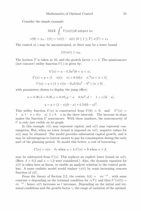
This utility function U(u) is constructed from U(0) = 0, and U ′(u) =1 − u, 1 − a + d(u − a), 1 + b − u in the three intervals. The increase in slopemakes the function U nonconcave. With these numbers, the nonconcavity ofU is only just visible on its graph.
In this example x(t) may represent capital, and u(t) may represent con-sumption, But, when no lower bound is imposed on u(t), negative values foru(t) may be obtained. The model provides substantial capital growth, and itmay be advantageous to borrow money to pay for consumption during the earlypart of the planning period. To model this better, a cost of borrowing :
C(u) = κ(u − δ) when u < δ, C(u) = 0 when u ≥ δ,
may be subtracted from U(u). This replaces an explicit lower bound on u(t).(Here, δ = 0.2 and κ = 1.3 were considered.) Also, the dynamic equation forx(t) is taken here as linear, to enable an analytic solution to the control prob-lem. A more realistic model would replace γx(t) by some increasing concavefunction of x(t).
From the theory of Section 2.2, the costate λ(t) = −σe−γt , with someconstant σ depending on the terminal condition for x(T ); and then U ′(u(t)) =σe−γt ; hence u(t) increases as t increases. Depending on the initial and ter-minal conditions and the growth factor γ, the range of variation of the optimal
22 Chapter 2
Figure 3 Utility function U(u)
Figure 4 Control in jump regime
Mathematics of Optimal Control 23
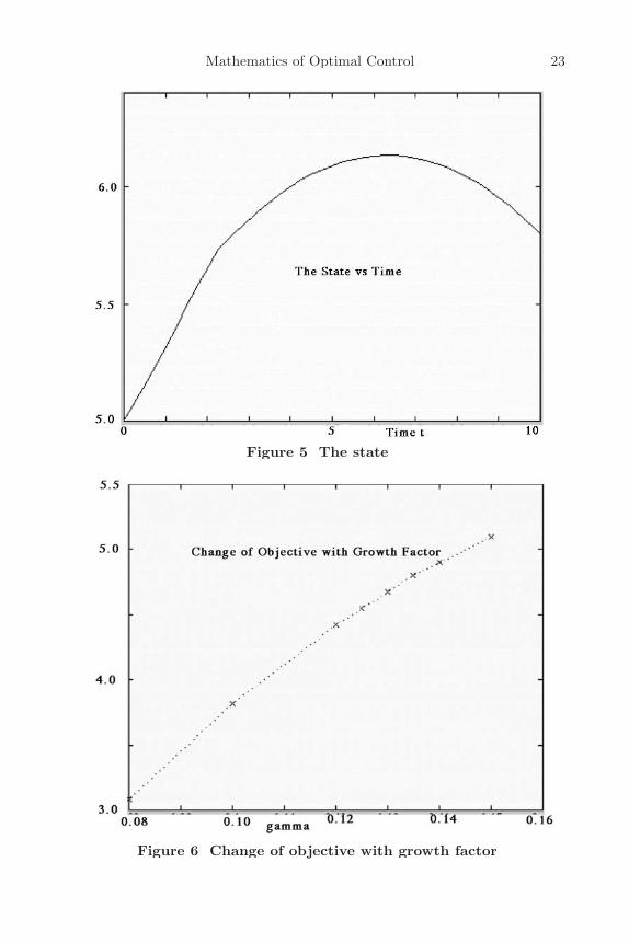
Figure 5 The state
Figure 6 Change of objective with growth factor
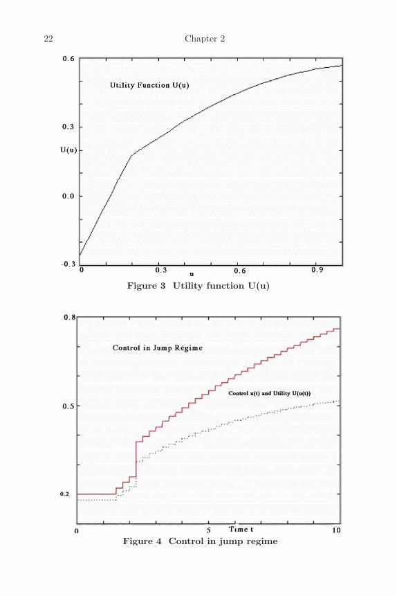
24 Chapter 2
u(t) may include the region where there are three possible solutions for u(t).Thus, there are two possible solution regimes, one where this region is notentered, so u(t) varies smoothly, and the second where u(t) jumps from theleftmost part of the U ′(t) curve to the rightmost part, at some level of u(t)depending on the parameters mentioned.
Computations with the SCOM optimal control package, described in chap-ter 3 (also Craven and Islam, 2001) confirm this conclusion. Figure 3 showsthe utility function, including the borrowing term. Figure 4 shows the optimalcontrol u(t), and the value of the utility U(u(t)), for one set of parameters(γ = 0.10, x0 = 5.0, xT = 5.80). In the computation, uj(t) was approximatedby a step-function with 40 subintervals; the theoretical solution would be asmooth curve, except for the jump at t = 2.3.
Figure 5 shows the state x(t); note the change in slope at t = 2, 3, whereu(t) jumps.
Figure 6 shows the change in the optimal objective as the growth factor γchanges, other parameters being the same. Note that the control u(t) changessmoothly when γ ≤ 0.13, whereas u(t) has a jump when γ > 0.13; the graphin Figure 6 changes slope at this level of γ.
2.7. Generalized dualityWhile duality requires convexity, or some weaker property such as invex,
there are relaxed versions of maximum for which quasiduality holds, giving ananalog of ZDG, but not weak duality. A point p is a quasimax of f(x), subjectto g(x) ≤ 0, if (Craven, 1977)
f(x) − f(p) ≤ o(‖x − p‖) whenever g(x) ≤ 0.
Here a function q(x) = o(‖x − p‖) when q(x)/‖x − p‖ → 0 when‖x − p‖ → 0.A function f has a quasimin at p if −f has a quasimax at p. If f and gare differentiable functions, and a constraint qualification holds, then (Craven,1997) p is a KKT point exactly when p is a quasimax.
Attach to the problem:
QUASIMAXxf(x) subject to g(x) ≤ 0
the quasidual problem:
QUASIMINu,vf(u) + vg(u) subject to v ≥ 0, f ′(u) + vg′(u) = 0.
Then (Craven, 1977, 1995) there hold the properties:• ZDG If x∗ is a quasimax of the primal (quasimax) problem, thenthere is a quasimin point (u∗, v∗) of the quasidual problem for whichf(x∗) = f(u∗) + v∗gf(u∗), thus the objective functions are equal.• perturbations if V (b) = QUASIMAXf(x) subject to g(x) ≥ 0,with the quasimax for b = 0 occurring at x = x∗, and if (u∗, v∗) are the

Mathematics of Optimal Control 25
optimal quasidual variables for which ZDG hold with f(x∗), then thequasi-shadow price vector V ′(0) = v∗.
There are several quasimax points with related quasimin points, and theycorrespond in pairs. These quasi properties reduce to the usual ones if −fand −g are invex with respect to the same scale function η(·). However, for anequality constraint k(x) = 0, the required invex property has = instead of ≥.
Simple examples of quasimax and quasidual are as follows.Example 1: (Craven, 1977) The quasidual of the problem:
QUASIMAXx − x +12x2 subject to x ≥ 0,
is:
QUASIMINu,v − u +12u2 + vu subject to − 1 + u + v = 0, v ≥ 0,
which reduces to the quasidual : QUASIMINu − 12u2 subject to u ≤ 1. The
primal problem has a quasimax at x = 0, with objective value 0, and a quasiminat x = 1, with objective value − 1
2 . The quasidual has a quasimin at u = 0with objective value 0, and a quasimin at u = 1 with objective value − 1
2 .
Example 2: Here, the quadratic objective may be a utility function forsocial welfare, not necessarily concave, to be maximized, subject to linear con-straints. The quasidual vectors are shadow prices. For given vectors c and s,and matrices A and R, suppose that the problem:
QUASIMAXz∈Rn F (z) := −cT z + (1/2)zT Az subject to z ≥ 0, Rz ≥ s,
reaches a quasimax at a point p where the constraint z ≥ 0 is inactive, and theconstraint Rz ≤ s is active. Then KKT conditions give Ap+RT λ = c, Rp = s,with multiplier λ ≥ 0. Setting z = p + v, F (z)− F (p) = −λT Rv − (1/2)vT Avwith Rv ≥ 0. So −λT Rv ≤ 0, and F (z)−F (p) may take either sign, dependingon the matrix A, so p is generally a quasimax, not a maximum. The associatedquasidual problem is:
QUASIMINu,v − cT u + (1/2)uT Au − vT (Tu − s) subject to
c − Au − RT v = 0, v ≥ 0.
However, the main applicability of quasimax is when the primal maxi-mization problem has several local maxima, as is likely to happen when theobjective function is far from concave. To each local maximum correspondsa quasimin of the quasidual, with the ZDG property, and quasidual variables,giving shadow prices. Thus the shadow price, for each local maximum, is anoptimum point of a quasimin problem.
26 Chapter 2
When there are equality constraints, the invex property takes a differentform. In general, a vector function F is invex with respect to a convex cone Qat a point p if:
(∀x) F (x) − F (p) ∈ F ′(p)η(x, p)
holds for some scale function η(., .). If some component h(x) of F (x) belongsto an equality constraint h(x) = 0, then the related part of Q is the zero point{0}; hence invex requires an equality:
(∀x) h(x) − h(p) = h′(p)η(x, p).
2.8. Multiobjective (Pareto) optimization5
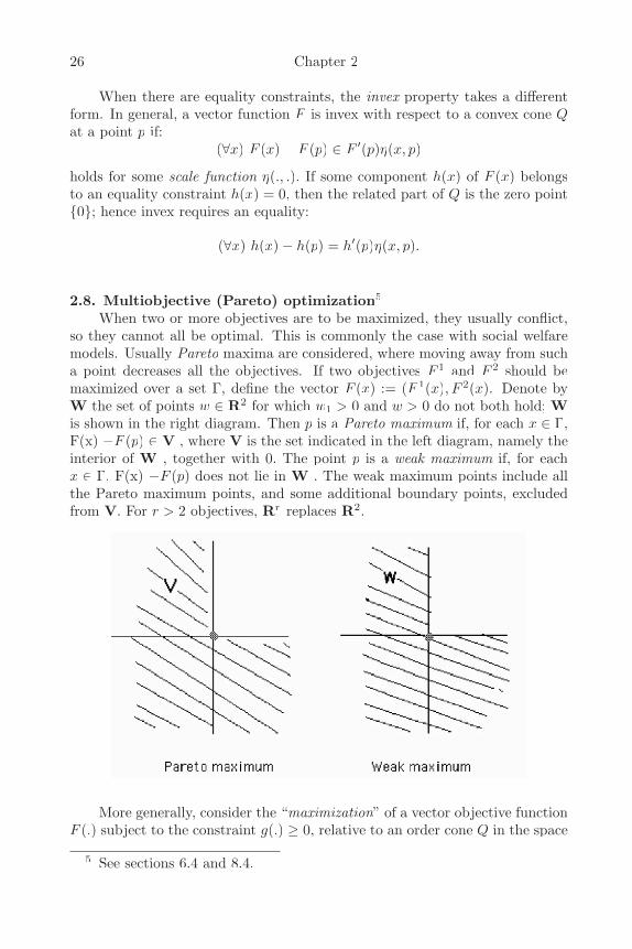
When two or more objectives are to be maximized, they usually conflict,so they cannot all be optimal. This is commonly the case with social welfaremodels. Usually Pareto maxima are considered, where moving away from sucha point decreases all the objectives. If two objectives F 1 and F 2 should bemaximized over a set Γ, define the vector F (x) := (F 1(x), F 2(x). Denote byW the set of points w ∈ R2 for which w1 > 0 and w > 0 do not both hold; Wis shown in the right diagram. Then p is a Pareto maximum if, for each x ∈ Γ,F(x) −F (p) ∈ V , where V is the set indicated in the left diagram, namely theinterior of W , together with 0. The point p is a weak maximum if, for eachx ∈ Γ, F(x) −F (p) does not lie in W . The weak maximum points include allthe Pareto maximum points, and some additional boundary points, excludedfrom V. For r > 2 objectives, Rr replaces R2.
More generally, consider the “maximization” of a vector objective functionF (.) subject to the constraint g(.) ≥ 0, relative to an order cone Q in the space
5 See sections 6.4 and 8.4.

Mathematics of Optimal Control 27
into which F maps. Denote by U the complement of the interior of Q. Apoint p is a weak quasimax of F (.), subject to g(.) ≥ 0, if for some functionq(x) = o(||x − p||), there holds:
F (x) − F (p) − q(x) ∈ U whenever g(x) ≥ 0.
(Note that weak maximum is the special case q(.) = 0.) Replacing U by theunion of 0 with the interior of U gives the slightly more restrictive Paretomaximum; a weak maximum may include a few additional boundary points.A weak quasimin of a vector function H is a weak quasimax of -H . If Fhas r components, then usually Q is taken as the orthant Rr.
+ The followingdiagram (see Craven, 1981) illustrates the definition, for the case when F hastwo components, so that the order cone Q is a sector, but not always the non-negative orthant R2
+. Such an ordering is appropriate when the consumers arenot isolated, as is discussed in section 8.2.
From Craven (1995), a (maximizing) weak Karush-Kuhn-Tucker point(WKKT) p satisfies:
τF ′(p) + λg′(p) = 0, λg(p) = 0, λ ≥ 0 τ ≥ 0, τe = 1.
Here τ is a row vector, e is a column vector of ones. The statement τ ≥ 0means, more precisely, that τ lies in the dual cone Q∗ of Q, defined by q∗(q) ≥ 0whenever q∗ ∈ Q∗ and q ∈ Q, If Q = Rr
+ then each component of τ is non-negative. There are many WKKT points, corresponding to different values ofτ.
Analogously to section 2.7 (and see Craven, 1990), the weak quasidual tothe (primal) problem:
WEAK QUASIMAXxF (x) subject to g(x) ≥ 0
has the form:
WEAK QUASIMINu,V F (u) + V g(u) subject to
28 Chapter 2
V (Rm+ ) ⊂ Q, (F ′(u) + V g′(u))(X) ⊂ U,
where the space X = Rn is the domain of F and g, and V is a r × m matrixvariable. The linearized problem about the point p:
QUASIMAX F ′(p)(x − p) subject to g(p) + g′(p)(x − p) ≥ 0
If a constraint qualification holds, and without any convex or invex as-sumption, there hold (Craven, 1989, 1990):
• p is a WKKT point exactly when p is a weak quasimin.• ZDG If x∗ is a weak quasimax point of the primal, with multipliersτ, λ, then there there is a weak quasimax point (u, V ) = (x∗, V ∗) of theweak quasidual problem, with τV ∗ = λ, and equal optimal objectives:
F (x∗) = F (u∗) + V ∗g(u∗).
Proof Let x and u, V be feasible for the respective problems. Then (usingquasidual constraints):
[F (u) + V g(u)] − [F (x∗) + V ∗g(x∗)) ∈ Q + [F (u) + V ∗g(u)]
−[F (x∗) + V ∗g(x∗) + (V − V ∗)(g(u) − g(x∗)}= Q + (F + V g)′(x∗)(u − x∗) + o(‖u − x∗‖) + (o(‖u − x∗‖) + o(‖V − V ∗‖)),
⊂ U + o(‖u − x∗‖ + ‖V − V ∗‖).• Linearization The linearized problem about p reaches a weak maximumat p.• Shadow prices If x∗ is a weak quasimax of the primal, then x∗ is alsoa quasimax of τ∗F (x); so the shadow prices for τ∗F are optimal for:
QUASIMAX F ′(p)(x − p) subject to g(p) + g′(p)(x − p) ≥ 0
• Multilinear problem (Bolinteanu and Craven, 1992) If F is linear, andg is linear (plus a constant), then p is stable to small perturbations, andthere is a shadow price for F for perturbations that do not change thelist of active constraints.
Example 3 - Vector quasimax and quasidual
WEAK QUASIMAXz∈Rn {FiFF (z)}ri=1 := {−cT
i z + (1/2)zT Aiiz}ri=1,
subject to Rz ≥ s,
for given vectors ci, d, s and matrices Ai, R; here {FiFF (z)}ri=1 specifies a vector
objective by its components. For each multiplier τ ≥ 0, with eT τ = 1, where eis a vector of ones, there corresponds a quasimax z = z(τ), with:
AT z(τ) + RT0 λ(τ) = c, R0z(τ) = s0,
Mathematics of Optimal Control 29
in which Roz ≥ s0 describes the constraints active at z(τ), c =∑
τiττ ci, A =∑τiττ Ai, As in example 2, this quasimax becomes a maximum if the matrix A is
restricted, e.g. to be negative definite in feasible directions. This problem maydescribe e.g. conflicting objectives of output and envoronmental quality forsustainable development, and requiring nonlinear functions to describe them.The vector quasidual is then:
WEAK QUASIMAXu,V {−ci + uT Ai}ri=1 + V R)(Rn) ⊂ U, V ≥ 0,
where U = Rr\ int Rr+; each component of V is ≥ 0.
While a quasimax is not generally a maximum, the quasi properties reduceto the standard properties if an additional assumption, such as convex or invex,is made. Consider the problem of weak maximization of F (x) < with respectto the order cone Q, subject to constraints g(x) ≥ 0 and k(x) = 0. In weakKKT, a term σk′(p) is added to λg′(p), where the multiplier σ is not restrictedin sign. The invex property stated in section 3.2 (see Hanson, 1980; Craven,1981; Craven, 1995) now takes the form:
−F (x) + F (p) + F ′(p)η(x, p) ∈ Q,
g(x) − g(p) ≤ g′(p)η(x, p),
k(x) − k(p) = k′(p)η(x, p),
for the same scale function η(x, p) in each case. (The inequalities derive froma cone-invex property H(x)−H(p)−H ′(p)η(x, p) ∈ Q×Rm
+ ×{0} for a vectorfunction H = −(F, g, k) (see Craven 1995).
In particular, if all components of F and g are concave, and all compo-nents of k are affine (constant plus linear), then invexity holds with η (x, p)= x−p, and the necessary conditions weak KKT, or equivalentlyTT weak quasimax,become also sufficient for a maximum. But these assumptions are often not ful-filled in applications. Some conditions when invexity holds are given in Craven(1995, 2000). A transformation x = ϕ (y) of the domain, where ϕ is invertible,with both ϕ and ϕ−1 differentiable, preserves the invex property, although thescale function is changed. The name invex derives (Craven, 1981) from invari-ant convex ; thus if a function H is convex, then the transformed function H◦ϕis invex (though not every invex function is of this form). However, for anequality constraint k( x ) = 0, k(.) is invex at p if k(x) − k(p) = k′(p)η (x, p),For KKT to be sufficient for an optimum, this invex property is only requiredfor those x where k(x) = 0. So the requirement reduces to the reduced invex(rinvex) property: k(x) = 0 = k′(p)η(x, p).
A multiobjective analog of saddlepoint was given in Craven (1990), andthe results are summarized here. The point p is a weak saddlepoint (WSP) (seeCraven, 1990) if:
τT F (p) + vT g(p) ≥ τT F (p) + λT g(p) ≥ τT F (x) + λT g(x)
30 Chapter 2
holds for all x, and all v ≥ 0. The multiplier τ (where 0 = τ ≥ 0) depends onp. The point p is a weak quasisaddlepoint if (given τ ):
(∀x,∀µ ≥ 0)τF (p) + µg(p) ≥ τF (p) + λg(p) ≥ τF (x) + λg(x) + o(‖x − p‖).
The following relations hold (Craven, 1995) for the vector function F on E andp ∈ E:
p is a Pareto maximum ⇒ p is a weak maximum
⇒ p is a weak quasimax
⇔ p is a weak KKT point (assuming regularity of the constraint)
⇔ p is a weak quasisaddlepoint .
Weak maximum (and weak quasimax) points may include some boundarypoints which lack a desired stability property. The statement that 0 = τ =(τ1, . . . , τrττ ) ≥ 0 means that all components τiττ ≥ 0, and they are not all zero. Ifτ > 0, namely if all τiττ > 0, then (Craven, 1990): weak KKT & τ > 0 ⇔ locallyproper weak quasimax , where locally proper means that ratios of deviations ofthe different Fi from Fip) are bounded (inequalities of Geoffrion, 1968) whenx is near p. These ratios represent tradeoffs between the objective components.They are approximated by the corresponding ratios of the τiττ . Thus a properquasimax occurs exactly when all the multipliers τiττ for the objectives are strictlypositive. This property does not require the Lagrange multipliers to be stated.As motivation, note that the stationary points of a real function f are the pointp where the gradient f ′(p) = 0; and maximum points are sought among thestationary points, If there are constraints, then constrained maximum pointsare among the KKT points instead of stationary points, A quasimax point pis a maximum point of the linear program, obtained by linearizing the givenproblem about the point p.
2.9. Multiobjective optimal controlFor an optimal control problem with a single objective, the KKT condi-
tions are essentially equivalent to an adjoint differential equation for a costatefunction, together with Pontryagin’s principle. This extends to multiobjectivecontrol problems.
Consider an optimal control problem, to find Pareto maximum points ofa vector objective F (x, u), subject to a dynamic equation that determines thestate x in terms of the control u, and other constraints. By substituting for xin terms of u, the problem takes the form:
PMAX J(u) subject to u ∈ U,
where PMAX denotes Pareto maximum, and the feasible set U is a closedbounded subset of some vector space V . Suppose that u ∈ U ⇔ G(u) ≤ 0,

Mathematics of Optimal Control 31
for some function G. If a Pareto maximum point u is reached, then (underrestrictions usually satisfied), multipliers τ and ρ exist such that Karush-Kuhn-Tucker (KKT) conditions hold:
τJ′(u) + ρG′(u) = 0, 0 = τ ≥ 0, ρ ≥ 0, ρG(u) = 0.
If −J and G satisfy some relaxed version of convexity, such as invexity (seeCraven, 1995), then the KKT conditions, in turn, imply a Pareto maximum,and also that τJ(u) is maximized, subject to G(u) ≤ 0, at u. Then each τcorresponds to one or more Pareto maximum points, and each Pareto max-imum point corresponds to one or more multipliers τ. If minimum points ofτJ(.), subject to G(u) ≤ 0, exist for each τ ≥ 0, then the existence of Paretomaximum points is established.
For an optimal control problem in continuous time, the vector space V isinfinite dimensional, so compactness properties of U are not generally available,so a Pareto maximum of a continuous vector function is not always reached.For each given τ, assume that J(u) := τJ(u) has a finite lower bound over U .If J(u) has the form
∫ T
0
∫∫f(x(t), u(t), t)dt, with a coercivity assumption on the
integrand f, that:
(∀x, u, t)f(x, u, t) ≥ g(u) , where g(u)/|u| → ∞ as |u| → ∞,
together with convexity of a set: ∪u∈U{ (z, y) : z = m(x, u, t)y ≥ f(x, u, t),where U is the closed set of values allowed to u(t), then a maximum for J(u)exists (see Fleming and Rishel, 1975, Theorem 4.1). But these assumptions areoften not satisfied for an economic growth model.
Suppose, however, that u = p is a solution of the KKT necessary con-ditions for a maximum of J(u) (or equivalently of the Pontryagin conditions− see section 2.2). Additional assumptions are needed, to ensure that p is amaximum. Suppose that S1 ⊂ S2 ⊂ . . . ⊂ Sn ⊂ . . . is an increasing sequence offinite-dimensional subspaces of V , and that p is a limit point of their union.Suppose also that each Sn ∩ U is bounded (in a finite dimension); then J(u)reaches a maximum, say at u = pn , over Sn ∩ U . Then J(pn) → J(p), andp is a maximum point for J. (See Craven (1999b) for an example for a controlmodel where bang-bang control is optimal.)
Otherwise, if u = p satisfies the Pontryagin conditions, and if the functionsof the problem satisfy invex conditions (see Craven 1995), then p is a maximum.In particular, it suffices if the integrand f of the objective is concave, andthe dynamic differential equation for the state is linear. Less restrictively, afunction ϕ is invex at p if :
ϕ(u) − ϕ(p) ≥ ϕ′(p)η(u, p),
where the scale function η must be the same for the several functions (-f andconstraint functions) describing the problem. But this is often not the case for
32 Chapter 2
a given dynamic equation. However, the control problem has a local maximumat p if −f is invex, under lesser restrictions on the differential equation (seesection 8.6.)
The maximum point p for J(u) is unique if the Pontryagin conditionshave a unique solution. This may happen, in particular (see Islam and Craven,2001b) when there are no control constraints, so that the Pontryagin maximumcondition reduces to a gradient equation, fuff +λmu = 0. If this equation definesu as a unique function of λ, and some Lipschitz conditions hold for f,m,mx
and mu , then the differential equations for x and λ (substituting for u) haveunique solutions.
For a multiobjective problem, the maximum point cannot be unique, butthe set of Pareto maximum points is unique, if one of the above criteria applies.
2.10. Multiobjective Pontryagin conditions6
Consider an optimal control problem, to find a Pareto (or weak) maximumfor two objective functions over a time interval [0, T] :
PMAX {∫ T
0
∫∫f1(x(t), u(t), t)dt + Φ1(x(T )),
∫ T
0
∫∫f2(x(t), u(t), t)dt + Φ2(x(T ))}
subject to:
x(0) = x0, x(t) = m(x(t), u(t), t) (0 ≤ t ≤ T ),
a(t) ≤ u(t) ≤ b(t) (0 ≤ t ≤ T ).
Here the state function x(.) and control function u(.) can be scalar or vectorvalued; PMAX denotes Pareto maximum; there may be endpoint contributionsΦ1,Φ2. Note that a Pareto minimum of {F 1, F 2} is a Pareto maximum of{−F 1,−F 2}. There can be more than two objectives.
The relevance of such models to economic growth, decentralization, socialchoice, and sustainable growth is discussed in chapters 5, 6 and 8. In particular,components of u(.) may represent consumption, and components of x(.) mayrepresent capital stock, with a dynamic differential equation describing eco-nomic growth. Questions of existence and uniqueness are discussed in sections2.3 and 2.5.
The above optimal control model can be described by a Hamiltonian :
h(x(t), u(t), t; τ, λ(t)) :=
6 See section 8.4.
Mathematics of Optimal Control 33∑
i
τiττ [f i(x(t), u(t), t) + δ(t − T )Φi(x(T ))] + λ(t)m(x(t), u(t), t)
Here λ(.) is the costate function ; τiττ are nonnegative multipliers; and the end-point terms Φi(x(T )) have been replaced by terms δ(t − T )Φi(x(T )) added tothe integrands; δ(.) is Dirac’s delta-function.
The analysis in Craven (1999a) uses a Lagrangian L(.) = h(.) + λ(t)x(t).The optimum is then described by the necessary Karush-Kuhn-Tucker
(KKT) conditions. From this is deduced, under some regularity assumptions,a (weak) adjoint differential equation:
λ(t) = τT fxff (x(t), u(t), t) + λ(t)mx(x(t), u(t), t), λ(T ) = τT Φ′(x(T )),
(where fxff denotes (∂/∂x)f, etc.), together with the Pontryagin principle:
h(x(t), ., t; τ, λ(t)) → MAX over [a(t), b(t)] at the optimal u(t).
There are many Pareto (or weak) optimal points, corresponding to variousvalues of τ, where 0 = τ ≥ 0. If the constraints on the controls are inactive,then MAX h implies:
hu(x(t), u(t), t; τ, λ(t)) = 0
at the optimal x(t), u(t), λ(t). (Note that this does not imply MAX h.)The costate function λ(t) represents a shadow price for the differential
equation. Thus, if the dynamic differential equation is perturbed to:
x(0) = x0, x(t) = m(x(t), u(t), t) − β(t),
where β(.) is a continuous function of small norm, then the change in theoptimal value of τf(.) is approximated by
∫ T
0
∫∫λ(t)β(t)dt.
An alternative description uses a vector Hamiltonian :
H(x(t), u(t), t; Λ(t)) :=
f(x(t), u(t), t) + δ(t − T )Φ(x(T )) + Λ(t)m(x(t), u(t), t),
in which f is the vector of f i,Φ is the vector of ϕi , and Λ(t) is a matrix valuedfunction instead of the vector function λ(.). The vector adjoint equation is then:
Λ(t) = fxff (x(t), u(t), t) + Λ(t)mx(x(t), u(t), t),Λ(T ) = Φ′(x(T )).
Corresponding to Pontryagin’s principle, there is a Pareto (or weak) optimumof the vector Hamiltonian, thus:
H(x(t), ., t; Λ(t)) → PMAX over [a(t), b(t)] at the optimal u(t).
34 Chapter 2
The maximum in Pontryagin’s principle becomes here a Pareto maximum.If the constraints on the controls are inactive, then optimizing the vector Hamil-tonion implies (for two objectives) that:
(∃τ ≥ 0, τ = 0) τHu(x(t), u(t), t; Λ(t)) = 0,
at the optimal x(t), u(t),Λ(t). (Note that this does not imply PMAX.)If multipliers τ and λ are known, then Λ(t) may be constructed from
τT Λ(t) = λ(t).
Chapter 3Computing Optimal Control :
The SCOM package
3.1. Formulation and Computational ApproachThis chapter discusses computational approaches to optimal control in
economics and finance, in particular for modelling social choice and publicdecision making. For the mathematical background, refer to sections 2.1 and2.2. A computing package called SCOM has been developed by the presentauthors, using MATLAB (see sections 3.3 and 3.4, and Craven and Islam,2001). Some applications are given in sections 3.6 and 3.7.
Consider an optimal control problem, of the form:
MINx(.),u(.) F 0(x, u) :=∫ 1
0
∫∫f(x(t), u(t), t)dt + Φ(x(1))
subject to x(0) = a, x(r) = m(x(t), u(t), t), q(t) ≤ u(t) ≤ r(t) 0 ≤ t ≤ 1).
Here the state function x(.), assumed piecewise smooth, and the control func-tion u(.), assumed piecewise continuous, are, in general, vector-valued; theinequalities are pointwise. A substantial class of optimal control problems can(see Teo et al., 1991; Craven, 1998) be put into this form; and, in many cases,the control function can be sufficiently approximated by a step-function. Aterminal constraint σ(x(1)) = b can be handled by replacing it by a penaltyterm added to F 0(x, u); thus the objective becomes:
F (x, u) := F 0(x, u) + 12µ‖σ(x(1)) − b∗‖2,
where µ is a positive parameter, and b∗ approximates to b.In the augmented Lagrangian algorithm (see e.g. Craven, 1995), con-
straints are thus replaced by penalty terms; µ is finite, and typically need notbe large; here b∗ = b + θ/µ, where θ is a Lagrange multiplier. If there arefew constraints (or one, as here), the problem may be considered as one ofparametric optimization, varying b∗, without computing the multipliers.
The differential equation, with initial condition, determines x(.) from u(.);denote this by x(t) = Q(u)(t); then the objective becomes:
J(u) = F 0(Q(u), u) + 12µ‖σ(Q(u)(1)) − b∗‖2,
For the formula to compute the gradient J ′(u) of the objective, refer to section2.1.
36 Chapter 3
A diversity of algorithms have been proposed for computing optimal con-trol. Algorithms for optimal control (Mufti, 1970, Teo et al., 1991) have beenvariously based on: (i) dynamic programming; (ii) solving first-order necessaryconditions of the Pontryagin theory; (iii) applying some approximation meth-ods (steady state solution, numerical methods based on approximation andperturbation, and method of simulation); (iv) approximating the control; and(v) applying mathematical programming algorithms to a discretized version ofthe control problem.
Many of these methods (especially methods (i) to (iii)) are based on thefirst order maximization conditions of a control problem, which Schwartz (1996)has called indirect methods. About the suitability of these methods for comput-ing optimal control, Schwartz (1996, p. 1) has made the following statement:
The main drawback to indirect methods is their extreme lack of robustness:the iterations of an indirect method must start close, sometimes very close,to a local solution in order to solve the two-point boundary value subproblems.Additionally, since first order optimality conditions are satisfied by maximisersand saddle points as well as minimizers there is no reason, in general, to expectsolutions obtained by indirect methods to be minimizers.
Against these indirect methods, he has advocated the superiority of thedirect methods, the principles of which, according to him are as follows (p. 1):
Direct methods obtain solutions through the direct minimization of the ob-jective function (subject to constraints) of the optimal control problem. In thisway the optimal control problem is treated as an infinite dimensional mathe-matical programming problem.
The superiority of this direct method or the control discretisation methodhas also been advocated and implemented increasingly by others in recent years(Craven, 1998 ; Teo et al., 1991). The direct method considers an optimal con-trol problem as an mathematical programming problem in infinite dimensions(see e.g. Tabak and Kuo, 1971), and then discretizes to permit computation.
The discretisation method has also several advantages: relatively large-scale and complicated optimal control problems can be solved by this approachand the method is relatively accurate and efficient compared to the indirectmethods.
For the above reasons, we have adopted the discretisation (step functionand spline) approach in this book. The two computer programs, SCOM andRIOTS 95, used in this chapter for numerical computation are also based onthis approach.
The problem must be put into the above standard form, for conveniencescaling the time interval to [0, 1].. As described in Craven, de Haas, and Wet-tenhall (1998), a nonlinear scaling of time is sometimes appropriate, to getgood accuracy when the horizon T is large, without excessive computation.
For SCOM, the interval [0, 1] is now divided into N equal subintervals,and u(t) the successive subintervals. Thus, the discretization is achieved byrestricting u(.) to such a step-function, and the optimization is over the values
Computing Optimal Control : The SCOM package 37
u1, u2, . . . , uN . Then, from the differential equation, x(.) is a polygonal function,determined by its values x0, x1, . . . , xN at the gridpoints t = 0, 1/N, 2/N, . . . , 1.Since, because of the jumps at gridpoints, the right hand side of the dynamicdifferential equation is now not a smooth function of t the differential equationsolver chosen must be suitable for such functions. From the standard theory,the gradient J ′(u) is given by:
J ′(u)z =∫ 1
0
∫∫(f + λ(t)m)u(x(t), u(t), t)z(t)dt,
where the costate function λ(.) satisfies the adjoint differential equation:
−λ(t) = (f + λ(t)m)x(x(t), u(t), t), |λ(1) = µ(x(1) − b∗).
(Here suffixes x and u denote gradients with respect to x(.) and u(.).
3.2. Computational requirementsThe computer package SCOM is compared with another computer pack-
age, RIOTS 95, which is also based on MATLAB. The algorithmic steps forthese two packages may be summarized as follows:
• SCOM: approximation based on a step function, a differential equationsolution based on Runge-Kutta method and optimisation based on aonjugate gradient search method.• RIOTS: package uses various spline approximations to do this, and solvesthe differential equations by Runge Kutta methods and the optimisationproblem by projected descent.In solving the adjoint differential equation , interpolation is required, to
estimate values of x(t) at times t between gridpoints. (In SCOM, linear inter-MMpolation was used.) Similarly,
∂J(u)/∂uj =∫ (j+1)/N
j/N
∫∫(f + λ(t)m)u(x(t), u(t), t)
requires either interpolation of x(t) and λ(t), or an Euler approximation ofthe integral. (SCOM uses the latter; it may be too approximate for someproblems.) Of course, the number N of subintervals can be increased, to getbetter precision.
The differential equation solver must handle discontinuities at gridpoints.Many standard solvers do not. For example, MATLAB 5.2 includes six ordinarydifferential equation (ODE) solvers, of which only one – designated for stiffdifferential equations – is useful for solving x(t) = u(t) when u(.) is a step-function. A better approach is to modify slightly the well-known fourth orderRunge-Kutta method. If t is in the subinterval [j/N, (j+1)/N ], then u(t) musttake the appropriate value uj , and not (for example) uj+1 when t = (j +1)/N .This is easily achieved by recording j as well as t. With this approach, there
38 Chapter 3
is no need to further divide the subintervals, in order to integrate. If moreprecision is required, the number N of subintervals may be increased. Notethat the given differential equation is solved forwards (starting at t = 0), andthe adjoint differential equation is solved backwards (starting at t = 1). Insolving the adjoint equation, x(t) must be interpolated between gridpoints; incomputing J ′(u), both x(t) and λ(t) must be interpolated; in both cases, linearinterpolation was used. More precision can be got by increasing N .
Once the differential equation for x(.) is solved, the objective J(u) becomesa function J(u1, u2, . . . , uN ) of N variables. The optimization may be done,either:
• by computing objective values, but not gradients; or• by also computing gradients, using the adjoint differential equation.
In either case, the computing package is required to optimize the objective,subject to simple bounds. (Bounds could also be handled using penalty terms.)
When as in some economic models (see e.g. Kendrick and Taylor, 1971),fractional powers of the functions occur, e.g. with the term x(t)β includedin m(x(t), u(t), t) with 0(β < 1, then the differential equation (2) will bringx(t) < 0 for some choices of u(.), causing the solver to crash. Of course, onlypositive values of x(t) have meaning in such models. Even without explicitconstraints on u(.), the requirement x(.) > 0 forms an implicit constraint,which does not have a simple form. In such a case, it may be better to usefinite-difference approximations to gradients, since they may be valid, as usefulapproximations, over a wider domain.
Every algorithm for numerical computation of such an optimal controlmodel requires some approximation of the control function u(t) by a vector onsome vector space of finite dimension (n say). For comparison, the RIOTS 95package uses various spline approximations to do this (Schwartz, 1996), andsolves the differential equations by projected descent methods. A simpler ap-proach, followed by the MISER3 package for optimal control (Jennings et al.,1998), approximates the control function by a step-function, then solves the dif-ferential equations by sequential quadratic programming. Conjugate gradientmethods may also be used. e.g. with OCIM (Craven, de Haas and Wetten-hall, 1998). Different implementations may behave differently, in particularif the function is only defined on a restricted domain, since an optimizationmethod may want to search outside that domain. While a step-function isapparently a crude approximation, it has been shown in various instances (seeTeo et al., 1991) to produce accurate results. The reason is that integratingthe dynamic equation x(t) = . . . to obtain x(t) is a smoothing operation, whichattenuates high-frequency oscillations. It is pointed out in Craven (1995) that,if this attenuation is sufficiently rapid, the result of step-function approxima-tions converges to the exact optimum as N → ∞.. Some assumption of thisqualitative kind is in any case necessary, in order to ensure that the chosen fi-nite dimensional approximations shall allow a good approximation to the exactoptimum.
Computing Optimal Control : The SCOM package 39
Computer programs which can be used for a wide variety of continuouscontrol problems have become available only recently (Amman, Kendrick, andRust, 1996; Cesar, 1994; Tapiero, 1998; Teo et al., 1991). There are some pack-ages which are well known to economists such as DUAL, MATHEMATICA,etc.; see references in Amman, Kendrick and Rust (1996). Craven (1995) coversthe theory and algorithm for optimal control with a list of possible computerprograms including the OCIM program. Cesar (1994) also has references tosome other computer programs. A recent survey of optimal control packagesis also given in Tapiero (1998). RIOTS is developed by Schwartz, Polak andChen (1997).
The various optimisation algorithms that some of the optimal control pro-grams encode are as follows:
• sequential quadratic programming (MISER, Jennings et al. 1991),MATLABs optimiser´ constr (MATLAB, 1997), and SCOM);• projected descent methods (RIOTS 95, Schwartz 1996).They can behave differently, in particular if the function is only defined on
a restricted domain, since an optimisation method may want to search outsidethat domain. For example, the RIOTS 95 package uses various spline approx-imations to do this, and solves the differential equations by projected descentmethods. A simpler approach, followed by the MISER3 package for optimalcontrol, approximates the control function by a step-function, then solves thedifferential equations by sequential quadratic programming. Conjugate gradi-ent methods may also be used (as in OCIM). Different implementations maybehave differently, in particular if the function is only defined over a restricteddomain, since an optimisation method may want to search outside that domain.While a step-function is apparently a crude approximation, it has been shownin various instances (e.g. Craven 1995; Teo et al. 1991) to produce accurateresults. The reason is that integrating the dynamic equation (x(t) = . . .) toobtain x(t) is a smoothing operation, which attenuates high-frequency oscilla-tions. It is pointed out in Craven (1995) that if this attenuation is sufficientlyrapid, the result of step-function approximations converges to the exact op-timum as N → ∞. Some assumption of this qualitative kind is in any casenecessary, in order to ensure that the chosen finite dimensional approximationsshall allow a good approximation to the exact optimum.
From the alternatives discussed above, RIOTS and SCOM were chosen,because:
• these two programs can solve, easily and conveniently, a large class ofoptimal control problems with various types of objective functionals,differential equations, constraints on the state and control functions, andterminal conditions (such as bang bang, minmax, and optimal time controlproblems; see for the theory Sengupta and Fanchon, 1969; Teo, Goh andWong, 1991) ,• they are based on a widely used mathematical package MATLAB, and• RIOTS is commercially available for research in this area.
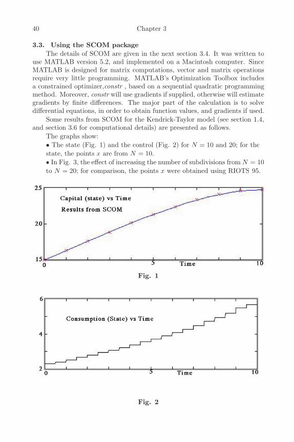
40 Chapter 3
3.3. Using the SCOM packageThe details of SCOM are given in the next section 3.4. It was written to
use MATLAB version 5.2, and implemented on a Macintosh computer. SinceMATLAB is designed for matrix computations, vector and matrix operationsrequire very little programming. MATLAB’s Optimization Toolbox includesa constrained optimizer,constr , based on a sequential quadratic programmingmethod. Moreover, constr will use gradients if supplied, otherwise will estimategradients by finite differences. The major part of the calculation is to solvedifferential equations, in order to obtain function values, and gradients if used.
Some results from SCOM for the Kendrick-Taylor model (see section 1.4,and section 3.6 for computational details) are presented as follows.
The graphs show:• The state (Fig. 1) and the control (Fig. 2) for N = 10 and 20; for thestate, the points x are from N = 10.• In Fig. 3, the effect of increasing the number of subdivisions from N = 10to N = 20; for comparison, the points x were obtained using RIOTS 95.
Fig. 1
Fig. 2

Computing Optimal Control : The SCOM package 41
Fig. 3
3.4. Detailed account of the SCOM package
3.4.1. PreambleSCOM is a computer package, using the constr program in MATLAB’s Op-
timization Toolbox, for solving optimal control problems in continuous time.The user must supply a calling program, and user subroutines for the functionsin the problem. There is a choice whether or not gradient subroutines are sup-plied. To supply them requires more mathematics and coding, gets much fastercomputation, but does not work with some control problems, if the functionsare only defined in a restricted domain. If gradients are not supplied, thenconstr can estimate them, but with less precision.
The MATLAB facilities make experimentation easy, since MATLAB doesmuch of the “housekeeping” (looping, matrix calculations, passing variables)that must be coded explicitly in some other languages.
3.4.2. Format of problem
Optimization is with respect to state x(t) and control u(t).
MINx(.),u(.)
∫ 1
0
∫∫f(x(t), u(t), t)dt + Φ(x(1)) subject to
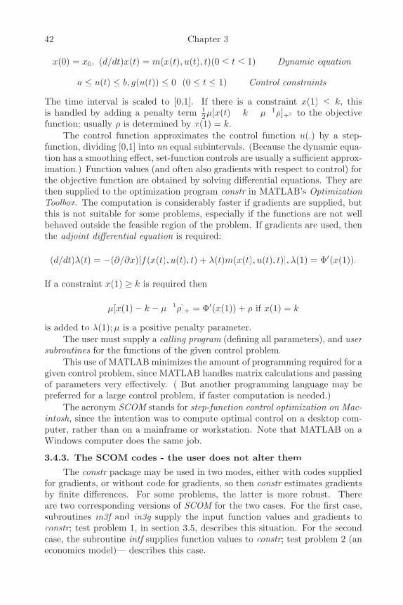
42 Chapter 3
x(0) = x0, (d/dt)x(t) = m(x(t), u(t), t)(0 ≤ t ≤ 1) Dynamic equation
a ≤ u(t) ≤ b, g(u(t)) ≤ 0 (0 ≤ t ≤ 1) Control constraints
The time interval is scaled to [0,1]. If there is a constraint x(1) ≤ k, thisis handled by adding a penalty term 1
2µ[x(t) − k − µ−1ρ]+2 to the objectivefunction; usually ρ is determined by x(1) = k.
The control function approximates the control function u(.) by a step-function, dividing [0,1] into nn equal subintervals. (Because the dynamic equa-tion has a smoothing effect, set-function controls are usually a sufficient approx-imation.) Function values (and often also gradients with respect to control) forthe objective function are obtained by solving differential equations. They arethen supplied to the optimization program constr in MATLAB’s OptimizationToolbox. The computation is considerably faster if gradients are supplied, butthis is not suitable for some problems, especially if the functions are not wellbehaved outside the feasible region of the problem. If gradients are used, thenthe adjoint differential equation is required:
(d/dt)λ(t) = −(∂/∂x)[f(x(t), u(t), t) + λ(t)m(x(t), u(t), t)], λ(1) = Φ′(x(1)).
If a constraint x(1) ≥ k is required then
µ[x(1) − k − µ−1ρ]+ = Φ′(x(1)) + ρ if x(1) = k
is added to λ(1);µ is a positive penalty parameter.The user must supply a calling program (defining all parameters), and user
subroutines for the functions of the given control problem.This use of MATLAB minimizes the amount of programming required for a
given control problem, since MATLAB handles matrix calculations and passingof parameters very effectively. ( But another programming language may bepreferred for a large control problem, if faster computation is needed.)
The acronym SCOM stands for step-function control optimization on Mac-intosh, since the intention was to compute optimal control on a desktop com-puter, rather than on a mainframe or workstation. Note that MATLAB on aWindows computer does the same job.
3.4.3. The SCOM codes - the user does not alter them
The constr package may be used in two modes, either with codes suppliedfor gradients, or without code for gradients, so then constr estimates gradientsby finite differences. For some problems, the latter is more robust. Thereare two corresponding versions of SCOM for the two cases. For the first case,subroutines in3f and in3g supply the input function values and gradients toconstr; test problem 1, in section 3.5, describes this situation. For the secondcase, the subroutine intf supplies function values to constr; test problem 2 (aneconomics model)— describes this case.
Computing Optimal Control : The SCOM package 43
% Get function values for constr - no gradient[f,g]=intf(uu,ps,q,xinit)[a,b,c]=ocf(uu,ps,q,xinit);f=a; g=b;
% Solve differential equations - no gradientsfunction [f,g,xm,f0]=ocf(um,ps,q,xinit)nx=ps(1);nu=ps(2);nn=ps(3);x0=xinit;xm=zeros(nx,nn+1); xm(:,1)=x0;ma=nx;t=0;it=1;hs=1/nn;px=char(q(1));xm=fnc(px,nx,nu,nn,xm,ma,t,it,hs,um,xm); %compute statema=1;t=0;it=1;hs=1/nn;zz=zeros(1,nn+1); zz(1)=0; pj=char(q(2));jm=fnc(pj,nx,nu,nn,zz,ma,t,it,hs,um,xm);%compute integralxf=xm(:,nn+1) ; pf=char(q(3));f=jm(nn+1) + feval(pf,xf); %objectivepc=char(q(4));for ii=1:nng(ii)=feval(pc,ii,hs,um,xm); % Control constraintendf0=jm(nn+1);f0;
% Organize steps for Runge-Kutta integration - no gradients casefunction xk=fnc(pd,nx,nu,nn,fil,ma,t,it,hs,um,xm)yin=fil(:,1);xk(:,1)=yin;while it ¡ nn+1y=rk4(pd,ma,t,it,hs,yin,nx,nu,nn,um,xm);xk(:,it+1)=y(1)’;it=y(2);t=y(3); yin=y(1);end
% Runge-Kutta incrementsfunction y=rk4(pd,ma,t,it,hs,yin,nx,nu,nn,um,xm)fp=zeros(1,ma);tt=zeros(1,ma); p=0; q=1;tz=ic2(pd,ma,t,it,hs,p,q,fp,yin,tt,um,xm);tt=tz(1); fp=tz(2);p=0.5;q=2;t=t+0.5*hs;tz=ic2(pd,ma,t,it,hs,p,q,fp,yin,tt,um,xm);tt=tz(1);fp=tz(2);tz=ic2(pd,ma,t,it,hs,p,q,fp,yin,tt,um,xm);
44 Chapter 3
tt=tz(1);fp=tz(2);t=t+0.5*hs;p=1;q=1;tz=ic2(pd,ma,t,it,hs,p,q,fp,yin,tt,um,xm);tt=tz(1);=tz(2);it=it+sign(hs);y=[yin+tt/6;it;t];
% Runge-Kutta - get function valuesfunction tz=ic2(pd,ma,t,it,hs,p,q,fp,yin,tt,um,xm)z=yin+p*hs*fp;ff=feval(pd,t,it,z,yin,hs,um,xm);fp=ff;tz=[tt+q*hs*fp;fp] ;
% Forward interpolationfunction ix=li3(vv,hh,xi)nn=length(vv)-1; nz=1/hh;fr=nz*mod(xi,hh); bb=floor(xi*nz)+1;if bb < nn, vu=vv(bb+1);else vu=vv(nn);endix=(1-fr)*vv(bb) + fr*vu;
% Backward interpolation (for adjoint DE)function ix=lil3(vv,hh,xi)global um xm jmnn=length(vv)-1; nz=-1/hh;if xi < 0, xi = 0; endfr=-nz*mod(xi,hh); bb=ceil(xi*nz)+1;if bb > 1, vw=vv(bb-1);else vw=vv(1);endix=(1-fr)*vv(bb) + fr*vw;
% Get function values for constr - gradients suppliedfunction [f,g]=in3f(uu,par,subs,xinit)[a1,a2,a3,a4,a5,a6]=ocf4(uu,par,subs,xinit); f=a1; g=a2;
% Get gradients for constrfunction [df,dg]=in3g(uu,par,subs,xinit)[a1,a2,a3,a4,a5,a6]=ocf4(uu,par,subs,xinit);df=a6; nn=par(3);pk=char(subs(5));dg=feval(pk,uu,nn);
% Solve differential equations - gradients supplied
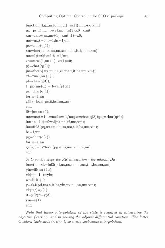
Computing Optimal Control : The SCOM package 45
function [f,g,xm,f0,lm,gr]=ocf4(um,ps,q,xinit)nx=ps(1);nu=ps(2);nn=ps(3);x0=xinit;xm=zeros(nx,nn+1); xm(:,1)=x0;ma=nx;t=0;it=1;hs=1/nn;px=char(q(1));xm=fnc(px,nx,nu,nn,xm,ma,t,it,hs,um,xm);ma=1;t=0;it=1;hs=1/nn;zz=zeros(1,nn+1); zz(1)=0;pj=char(q(2));jm=fnc(pj,nx,nu,nn,zz,ma,t,it,hs,um,xm);xf=xm(:,nn+1) ;pf=char(q(3));f=jm(nn+1) + feval(pf,xf);pc=char(q(4));for ii=1:nng(ii)=feval(pc,ii,hs,um,xm);endf0=jm(nn+1);ma=nx;t=1;it=nn;hs=-1/nn;pa=char(q(8));pq=char(q(6));lm(nn+1,:)=feval(pa,nn,xf,um,xm);lm=fnl3(pq,nx,nu,nn,lm,ma,t,it,hs,um,xm);hs=1/nn;pg=char(q(7));for ii=1:nngr(ii,:)=hs*feval(pg,ii,hs,um,xm,lm,nn);end
% Organize steps for RK integration - for adjoint DEfunction xk=fnl3(pd,nx,nu,nn,fil,ma,t,it,hs,um,xm)yin=fil(nn+1,:);xk(nn+1,:)=yin;while it ¿ 0y=rk4(pd,ma,t,it,hs,yin,nx,nu,nn,um,xm);xk(it,:)=y(1);it=y(2);t=y(3);yin=y(1);end
Note that linear interpolation of the state is required in integrating theobjective function, and in solving the adjoint differential equation. The latteris solved backwards in tine t, so needs backwards interpolation.
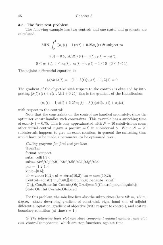
46 Chapter 3
3.5. The first test problemThe following example has two controls and one state, and gradients are
calculated.
MIN∫ 1
0
∫∫[(u1(t) − 1)x(t) + 0.25u2(t)]dt subject to
x(0) = 0.5, (d/dt)x(t) = x(t)u1(t) + u2(t),
0 ≤ u1 (t), 0 ≤ u2(t), u1(t) + u2(t) − 1 ≤ 0 (0 ≤ t ≤ 1).
The adjoint differential equation is:
(d/dt)λ(t) = −(1 + λ(t))u1(t) + 1, λ(1) = 0
The gradient of the objective with respect to the controls is obtained by inte-grating [λ(t)x(t) + x(t), λ(t) + 0.25]; this is the gradient of the Hamiltonian:
(u1(t) − 1)x(t) + 0.25u2(t) + λ(t)[x(t)u1(t) + u2(t)]
with respect to the controls.Note that the constraints on the control are handled separately, since the
optimizer constr handles such constraints. This example has a switching timeof exactly t = 0.75. This is only approximated with N = 10 subdivisions; someother initial control u gave a positive u(t) in subinterval 8. While N = 20subintervals happens to give an exact solution, in general the switching timewould have to be made a parameter, to be optimized over.
Calling program for first test problem%run3.mformat compactsubs=cell(1,9);subs=’t3x’,’t3j’,’t3f’,’t3c’,’t3k’,’t3l’,’t3g’,’t3a’;par = [1 2 10];xinit=[0.5];u0 = zeros(10,2); ul = zeros(10,2); uu = ones(10,2);Control=constr(’in3f’,u0,[],ul,uu,’in3g’,par,subs, xinit)[Obj, Con,State,Int,Costate,ObjGrad]=ocf4(Control,par,subs,xinit);State,Obj,Int,Costate,ObjGrad
For this problem, the subs line lists also the subroutines (here t3k.m, t3l.m,63g.m, t3a.m describing gradient of constraint, right hand side of adjointdifferential equation, gradient of objective (with respect to control), and costateboundary condition (at time t = 1.)
% The following lines plot one state component against another, and plottwo control components, which are step-functions, against time
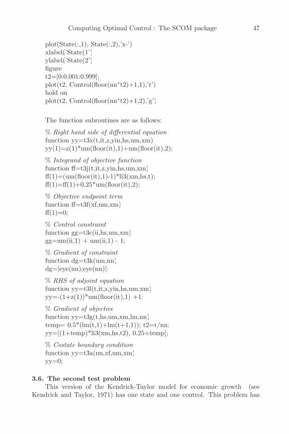
Computing Optimal Control : The SCOM package 47
plot(State(:,1), State(:,2),’x-’)xlabel(’State(1’)ylabel(’State(2’)figuret2=[0:0.001:0.999];plot(t2, Control(floor(nn∗t2)+1,1),’r’)hold onplot(t2, Control(floor(nn∗t2)+1,2),’g’)
The function subroutines are as follows:
% Right hand side of differential equationfunction yy=t3x(t,it,z,yin,hs,um,xm)yy(1)=z(1)*um(floor(it),1)+um(floor(it),2);
% Integrand of objective functionfunction ff=t3j(t,it,z,yin,hs,um,xm)ff(1)=(um(floor(it),1)-1)*li3(xm,hs,t);ff(1)=ff(1)+0.25*um(floor(it),2);
% Objective endpoint termfunction ff=t3f(xf,um,xm)ff(1)=0;
% Control constraintfunction gg=t3c(ii,hs,um,xm)gg=um(ii,1) + um(ii,1) - 1;
% Gradient of constraintfunction dg=t3k(um,nn)dg=[eye(nn);eye(nn)];
% RHS of adjoint equationfunction yy=t3l(t,it,z,yin,hs,um,xm)yy=-(1+z(1))*um(floor(it),1) +1;
% Gradient of objectivefunction yy=t3g(t,hs,um,xm,lm,nn)temp= 0.5*(lm(t,1)+lm(t+1,1)); t2=t/nn;yy=[(1+temp)*li3(xm,hs,t2), 0.25+temp];
% Costate boundary conditionfunction yy=t3a(nn,xf,um,xm)yy=0;
3.6. The second test problemThis version of the Kendrick-Taylor model for economic growth (see
Kendrick and Taylor, 1971) has one state and one control. This problem has

48 Chapter 3
implicit constraints, and a computation with gradient formulas supplied failed.(The dynamic equation ran x(t) into negative values, yet fractional powersof x(t) were required.) An optimum was computed using constr to estimategradients by finite differences.
With capital stock at time t as state function, and rate of consumption attime t as the control function, this model has the form:
MAX
∫ T
0
∫∫e−ρtu(t)τdt subject to
x(0) = k0, x(t) = ζeδtx(t)β − σx(t) − u(t), x(T ) = kT .
To allow comparison with numerical results in Kendrick and Taylor (1971), thefollowing numerical values were used:
T = 10, τ = 0.1, k0 = 15.0, ζ = 0.842, β = 0.6, σ = 0.05, kT = 24.7.
Although this model states no explicit bounds for x(t) and u(t), both the for-mulas and their interpretation requires that both x(t) and u(t) remain positive.But with some values of u(.), the differential equation for x(t) can bring x(t)down to zero; so there are implicit constraints.
This example was computed as a minimization problem, with N = 10 andN = 20 subdivisions (the latter required reduced termination tolerance andmore iterations). The different computations differed very little in the optimumobjective value. Evidently, the optimum objective here is fairly insensitive tosmall changes in the control. The convergence to an optimum objective valueis fast, but the convergence to an optimal control is slow. There is some scopehere for adjusting, within constr, the termination tolerances for gradient andfor satisfying constraints. Because of a difficulty with the fractional powers, thisproblem was computed with gradients obtained by constr from finite differences,instead of using gradients from the costate equation.
Calling program for second test problem%kt2run.mformat compactsubs=cell(1,4); subs=’kx’,’kj’,’kf’,’kc’;par=[1 1 10 15]; % 1 state, 1 control, 10 subintervale,ul=ones(10,1); % control lower bound is 1.0uh=10*ones(10,1); % control upper bound is 10.0xinit=[15]; % Initial stateu0=ones(1,10);Control=constr(’intf’,u0,[],ul,uh,[],par,subs,xinit)[Objective, Constraint, State, Integral]=ocf(Control,par,subs,xinit);Objective, State, Integral
Note that the subroutines (kx.m, kj,m, kf.m, kc.m) for the functions spec-ifying the problem, namely the right hand side of the differential equation,
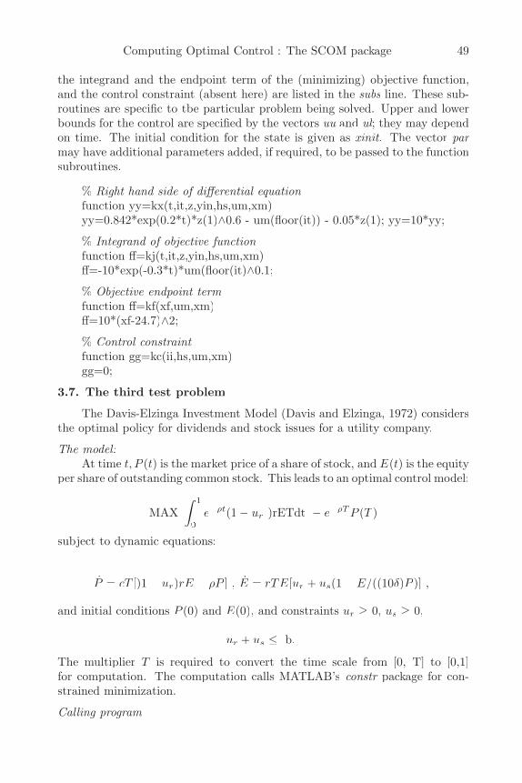
Computing Optimal Control : The SCOM package 49
the integrand and the endpoint term of the (minimizing) objective function,and the control constraint (absent here) are listed in the subs line. These sub-routines are specific to tbe particular problem being solved. Upper and lowerbounds for the control are specified by the vectors uu and ul; they may dependon time. The initial condition for the state is given as xinit. The vector parmay have additional parameters added, if required, to be passed to the functionsubroutines.
% Right hand side of differential equationfunction yy=kx(t,it,z,yin,hs,um,xm)yy=0.842*exp(0.2*t)*z(1)∧0.6 - um(floor(it)) - 0.05*z(1); yy=10*yy;
% Integrand of objective functionfunction ff=kj(t,it,z,yin,hs,um,xm)ff=-10*exp(-0.3*t)*um(floor(it)∧0.1;
% Objective endpoint termfunction ff=kf(xf,um,xm)ff=10*(xf-24.7)∧2;
% Control constraintfunction gg=kc(ii,hs,um,xm)gg=0;
3.7. The third test problem
The Davis-Elzinga Investment Model (Davis and Elzinga, 1972) considersthe optimal policy for dividends and stock issues for a utility company.
The model:At time t, P (t) is the market price of a share of stock, and E(t) is the equity
per share of outstanding common stock. This leads to an optimal control model:
MAX∫ 1
0
∫∫e−ρt(1 − ur )rETdt − e−ρT P (T )
subject to dynamic equations:
P = cT [)1 − ur)rE − ρP ] , E = rTE[ur + us(1 − E/((10δ)P )] ,
and initial conditions P (0) and E(0), and constraints ur ≥ 0, us ≥ 0,
ur + us ≤ b.
The multiplier T is required to convert the time scale from [0, T] to [0,1]for computation. The computation calls MATLAB’s constr package for con-strained minimization.
Calling program

50 Chapter 3
% dn2 run.m The calling program, setting the parameterssubs=cell(1,9);subs={’dnx’,’dnj’,’dnf’,’dnc’};par=[2, 2, 20, 0, 0, 1, 6, 0.2, 0.1, 0.1, 0.75]; % Parameters% nx, nu, nn, npa, grad, c, T, r, p, d, b=k/rxinit=[2 1]; nn=par(3);u0=zeros(nn,2);ul=zeros(nn,2);uu=ones(nn,2); figureControl=constr(’fqq’,u0,[],ul,uu,[],par,subs,xinit)[Objective,Constraint,State,Integral]= cqq(Control,par,subs,xinit)plot(State(:,1),State(:,2),’x-’) % Graph outputsxlabel(’State 1’)ylabel(’State 2’)figuret2=[0:.001:0.999];plot(t2,Control(floor(nn*t2)+1,1),’r’)hold onplot(t2,Control(floor(nn*t2)+1,2),’g’)
User subroutines
function ff= dnx(t,it,z,yin,hs,um,xm,ps)% The right hand sides of the DEs
c=ps(6);T=ps(7);r=ps(8);p=ps(9);d=ps(10);b=ps(11);ff(1)=c*T*((1-um(floor(it),1))*r*z(2)-p*z(1));temp=um(floor(it),2)*(1-z(2)/((1-d)*z(1)));ff(2)=r*T*z(2)*(um(floor(it),1)+temp);
function ff= dnj(t,it,z,yin,hs,um,xm,ps) % The integrandc=ps(6);T=ps(7);r=ps(8);p=ps(9);d=ps(10);b=ps(11);temp=iqq(xm,hs,t);ww=temp(2);ff(1)=-(1-um(floor(it),1))*r*T*ww*exp(-p*T*t);
function gg= dnc(ii,hs,um,xm,ps) % The constraints on the controlc=ps(6);T=ps(7);r=ps(8);p=ps(9);d=ps(10);b=ps(11);gg(1) = um(floor(ii),1)+um(floor(ii),2)-b;
function ff= dnf(xf,um,xm,ps) % Endpoint term of objectivec=ps(6);T=ps(7);r=ps(8);p=ps(9);d=ps(10);b=ps(11);ff(1)=-xf(1)*exp(-p*T);
Computed output, showing the effect of initial conditions on P and ENote that the theoretical solution is bang-bang control , thus the control
vector (ur, us ) switches between three regimes´ A = (0, 0), B = (b, 0), C =(0, b).), which are the vertices of the triangular region to which (ur, us) isrestricted. From the theory, the optimum switches from B to A if P (T )/E(T ) <
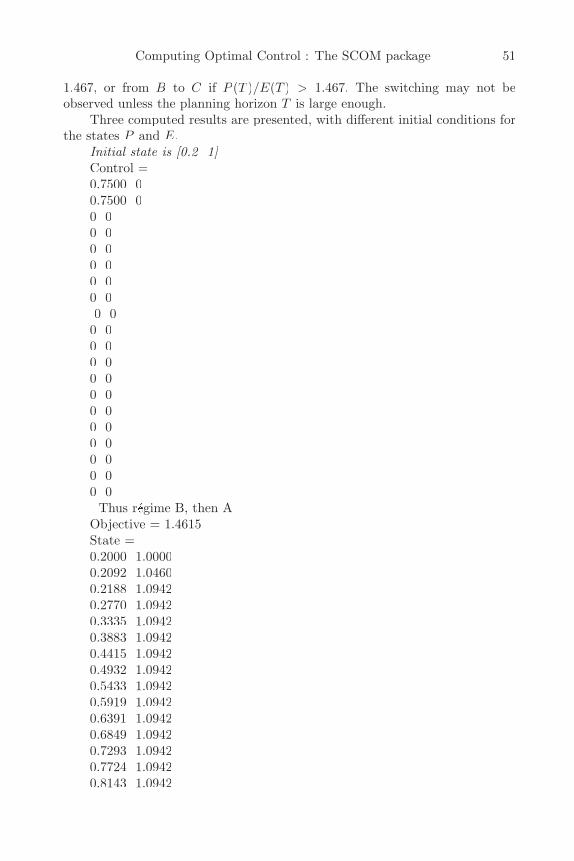
Computing Optimal Control : The SCOM package 51
1.467, or from B to C if P (T )/E(T ) > 1.467. The switching may not beobserved unless the planning horizon T is large enough.
Three computed results are presented, with different initial conditions forthe states P and E.
Initial state is [0.2 1]Control =0.7500 00.7500 00 00 00 00 00 00 00 0
0 00 00 00 00 00 00 00 00 00 00 0
Thus regime B, then A´Objective = 1.4615State =0.2000 1.00000.2092 1.04600.2188 1.09420.2770 1.09420.3335 1.09420.3883 1.09420.4415 1.09420.4932 1.09420.5433 1.09420.5919 1.09420.6391 1.09420.6849 1.09420.7293 1.09420.7724 1.09420.8143 1.0942
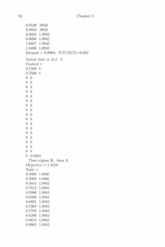
52 Chapter 3
0.8549 .09420.8943 .09420.9325 1.09420.9696 1.09421.0057 1.09421.0406 1.0942Integral = 0.8904; P(T)/E(T)=0.952
Initial state is [0.5 1]Control =0.7500 00.7500 00 00 00 00 00 00 00 00 00 00 00 00 00 00 00 00 00 00 0.0294
Thus regime B , then A´Objective = 1.5518State =0.5000 1.00000.5003 1.04600.5014 1.09420.5512 1.09420.5996 1.09420.6466 1.09420.6921 1.09420.7363 1.09420.7793 1.09420.8209 1.09420.8613 1.09420.9005 1.0942
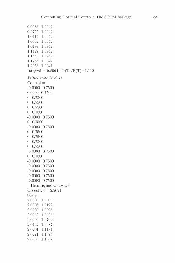
Computing Optimal Control : The SCOM package 53
0.9386 1.09420.9755 1.09421.0114 1.09421.0462 1.09421.0799 1.09421.1127 1.09421.1445 1.09421.1753 1.09421.2053 1.0941Integral = 0.8904; P(T)/E(T)=1.112
Initial state is [2 1]Control =-0.0000 0.75000.0000 0.75000 0.75000 0.75000 0.75000 0.7500-0.0000 0.75000 0.7500-0.0000 0.75000 0.75000 0.75000 0.75000 0.7500-0.0000 0.75000 0.7500-0.0000 0.7500-0.0000 0.7500-0.0000 0.7500-0.0000 0.7500-0.0000 0.7500
Thus regime C always´Objective = 2.2621State =2.0000 1.00002.0006 1.01992.0023 1.03982.0052 1.05952.0092 1.07922.0142 1.09872.0201 1.11812.0271 1.13742.0350 1.1567
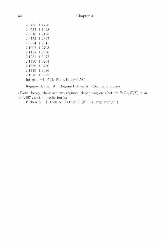
54 Chapter 3
2.0438 1.17582.0535 1.19482.0640 1.21382.0753 1.23272.0874 1.25152.1002 1.27032.1138 1.28902.1281 1.30772.1430 1.32642.1586 1.34502.1749 1.36362.1918 1.3822Integral =1.0592; P(T)/E(T)=1.586
Regime B, then A R´´ egime B then A R´´ egime C always´
(From theory, there are two regimes, depending on whether´ P (T )/E(T ) < or> 1.467 ; so the prediction is:
B then A, B then A B then C (if T is large enough )

Chapter 4Computing Optimal Growthand Development Models
4.1. IntroductionMethods and models for optimal growth and development are often for-
mulated as optimal control problems. They can represent a classical exampleof a social choice problem in an economy. Such models may describe intertem-poral allocation of resources, so as to maximize social welfare, determined onthe basis of the underlying social preferences and value judgements. They maydescribe a national economy, with state functions being vector valued, sincevarious commodities are involved. The consumption may be varied, withinsome limits, to optimise some utility functional, which may involve both stateand control functions over a planning period. In these models, there are ingeneral explicit bounds (such as floor to consumption, or a ceiling to capitalor pollution), as well as discontinuous control functions. These social choicemodels for optimal growth and development can be specified, and mumericallyimplemented, following the assumptions of new3 welfare economics, discussedin chapter 1.
Analytic solutions are available for some of the simpler models. Oftensome sort of steady state has been studied, but not the rate of approach tothe steady state from given initial conditions, or the transition to give terminalconditions (such as, for example, a stated minimum for terminal capital, sothat a process may continue). It is noted that the available data are necessarilyin discrete time (i.e. annual or quarterly data). While discrete-time optimalcontrol models can of course be computed, a continuous-time model may give amore intelligible picture of what is happening. Also, the Pontryagin theory foroptimal control applies to optimal control in continuous time, but only underserious restrictions to optimal control in discrete time. This chapter will henceconsider continuous-time models.
A computer package allows exploration of sensitivity to parameter changes,and of the domains of the various parameters for which optimal solutions exist.Some recently developed computer packages, coding different algorithms forcontinuous optimal control, such as RIOTS, MISER and OCIM, (which useMATLAB), have current applications to other areas of control, but have notyet been used for computing optimal growth models. The objective of thischapter is to demonstrate the applications of these algorithms and computerprograms to the computation of optimal growth models. The MATLAB pack-age SCOM, described in chapter 3, is used to study the Kendrick and TaylorMMmodel (Kendrick & Taylor, 1971). The computational results are consistentwith the economic conclusions obtained by these authors, and by Chakravarty
56 Chapter 4
(1969), and also with results computed with another package. With this com-putational simulation, it is easy to study the sensitivity of the results to changesin model parameters.
In addition, the optimum obtained has been proved to be the global opti-mum, using invexity properties (see section 2.4). The global optimality of themodel results is also proved in this chapter.
The chapter is organised as follows. Section 2 presents a Ramsey type(Ramsey, 1928), optimal growth model developed by Kendrick and Taylor(1971) and its optimal control specification. Section 3 discusses different al-gorithms and computer programs for solving optimal control models, whileSection 4 discusses the Kendrick-Taylor model and numerical implementationby some computer programs. Mathematical properties of the model results andthe sensitivity studies are reported in Section 5 respectively. Section 6 refers tothe experiences for computing optimal growth models by computer programs,such as OCIM and MISER. Section 7 contains the conclusion.
4.2. The Kendrick-Taylor Growth Model7
The well known Kendrick-Taylor model for economic growth and develop-ment (Kendrick and Taylor, 1971) has been used as a test problem for compu-tational approaches. With capital stock k(t) at time t as the state function,and rate of consumption c(t) at time t as the control function, this model hasthe form:
MAX∫ T
0
∫∫e−ρtc(t)τdt subject to:
k(0) = k0, k(t) = ζeqtk(t)β − σk(t) − c(t), k(T ) = kT .
This model does not state any explicit bounds for k(t) and c(t). However,both the formulas and their interpretation requires that both k(t) and c(t)remain positive. However, with some values of u(t), the differential equationfor k(t) can bring k(t) down to zero.
Consistent with the mainstream practice in modelling optimal growth,development and welfare economics, the numerical optimal growth programsin this chapter are specified within the framework of the elements of an optimalgrowth program of the following form: an optimality criterion contained in anobjective function which consists of the discounted sums of the utilities providedby consumption at every period; the finite planning horizon; a positive discountrate; and the boundary conditions given by the initial values of the variablesand parameters and by the terminal conditions.
This model can be expressed by a standard kind of optimal control model,which may be written as follows:
MINk(.),c(.)
∫ T
0
∫∫f(k(t), c(t), t)dt + Φ(k(T )) subject to
7 See also section 2.1.
Computing Optimal Growth and Development Models 57
k(0) = k0, k(t) = m(k(t), c(t), t), kL(t) ≤ k(t) ≤ kU (t) (0 ≤ t ≤ T ).
Here:f(k(t), c(t), t) = −e−ρtc(t); Φ(k(T )) = µ(k(T ) − k∗)2,
(with a minus sign on f to convert to a minimization problem), and:
m(k(t), (((t), t) = ζeδtk(t)β − σk(t) − c(t).
The terminal constraint for k(T ) has been replaced by a penalty cost termΦ(k(T )), with a parameter k∗ (approximately kT , but may need adjustment),and a sufficiently large coefficient µ. In general (though not for the presentinstance), k(t) and c(t) are vector valued.
The relevant mathematical issues that are investigated in the context of anoptimal growth model are the following: existence, uniqueness and globalityof the optimal policy solution, and stability of the dynamic system in theequilibrium or steady state position (Intriligator 1971).
The control issues of analytical and policy importance in control modelsare stated by Sengupta and Fanchon (1997) as: estimability, controllability,reachability, and observability. As these characteristics of control models relateto models with linear dynamics, but not to nonlinear systems, they are notinvestigated here. However, some numerical data relating to controllability aregiven in Section 4.4.
The Kendrick-Taylor model was numerically implemented by Kendrickand Taylor (1971) by several algorithms such as search and quasi- linearisationmethods based on the discrete Pontryagin maximum principle. In another ex-periment, Keller and Sengupta (1974) solved the model by conjugate search andDavidson algorithm based on the continuous Pontryagin maximum principle.While these algorithms were implemented by some special purpose computerprograms, a GAMS version (a general purpose commercially available program)of the Kendrick-Taylor model is also available.
4.3. The Kendrick-Taylor Model ImplementationTo allow comparison with numerical results in Kendrick and Taylor (1971),
the following numerical values were used:
T = 10, τ = 0.1, ζ = 0.842, β = 0.6, σ = 0.05, kT = b = 24.7.
The Kendrick-Taylor model, with the parameter values listed above, hasbeen computed using the RIOTS 95 package on a Pentium, and also with someof the parameters varied, as listed below. For comparison, the model has alsobeen computed using the SCOM package on an iMac computer. The latterpackage also uses MATLAB (version 5.2) and the constrained optimisationsolver constr from MATLAB’s Optimisation Toolbox, but none of the differ-ential equation software used by RIOTS 95. Thus both computations share
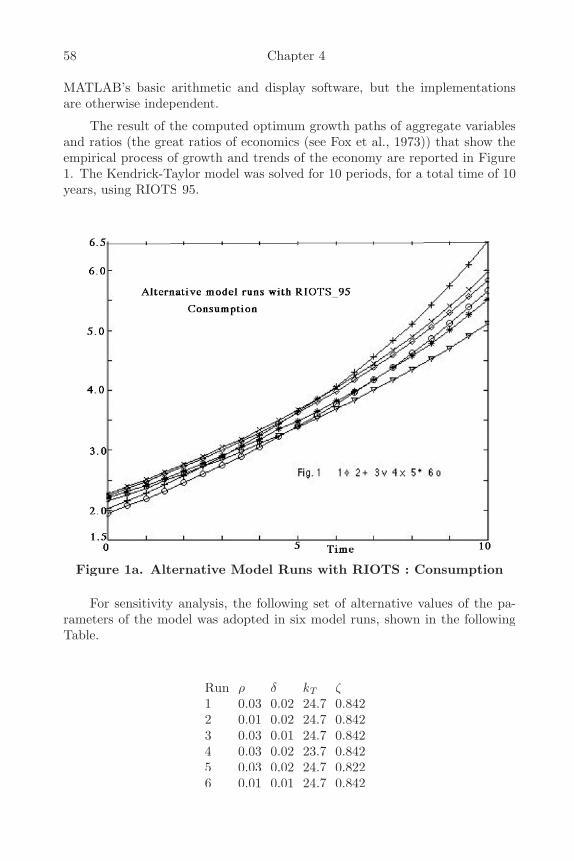
58 Chapter 4
MATLAB’s basic arithmetic and display software, but the implementationsare otherwise independent.
The result of the computed optimum growth paths of aggregate variablesand ratios (the great ratios of economics (see Fox et al., 1973)) that show theempirical process of growth and trends of the economy are reported in Figure1. The Kendrick-Taylor model was solved for 10 periods, for a total time of 10years, using RIOTS 95.
Figure 1a. Alternative Model Runs with RIOTS : Consumption
For sensitivity analysis, the following set of alternative values of the pa-rameters of the model was adopted in six model runs, shown in the followingTable.
Run ρ δ kT ζ1 0.03 0.02 24.7 0.8422 0.01 0.02 24.7 0.8423 0.03 0.01 24.7 0.8424 0.03 0.02 23.7 0.8425 0.03 0.02 24.7 0.8226 0.01 0.01 24.7 0.842
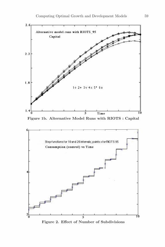
Computing Optimal Growth and Development Models 59
Figure 1b. Alternative Model Runs with RIOTS : Capital
Figure 2. Effect of Number of Subdivisions
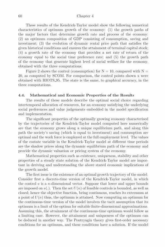
60 Chapter 4
These results of the Kendrick-Taylor model show the following numericalcharacteristics of optimum growth of the economy: (1) the growth paths ofthe major factors that determine growth rate and process of the economy;(2) an optimum composition of GDP consisting of consumption, saving andinvestment; (3) the evolution of dynamic rental price path that satisfies thegiven historical conditions and ensures the attainment of terminal capital stock;(4) a growth rate of the economy that provides a net rate of return of theeconomy equal to the social time preference rate; and (5) the growth pathof the economy that generate highest level of social welfare for the economy,obtained with the three computations.
Figure 2 shows the control (consumption) for N = 10, compared with N =20, as computed by SCOM. For comparison, the control points shown x wereobtained with RIOTS 95. The state is the same, to graphical accuracy, in thethree computations.
4.4. Mathematical and Economic Properties of the ResultsThe results of these models describe the optimal social choice regarding
intertemporal allocation of resources, for an economy satisfying the underlyingsocial preferences and value judgements embedded in the model specificationand implementation.
The significant properties of the optimally growing economy characterisedby the trajectories of the Kendrick-Taylor model computed here numericallyare that the economy grows along a unique equilibrium path, and along thispath the society’s saving (which is equal to investment) and consumption areoptimal and the work force is employed at the full employment level. The valuesof the costate variable in the Kendrick-Taylor model at different time periodsare the shadow prices along the dynamic equilibrium path of the economy andprovide the dynamic valuation or pricing system of the economy.
Mathematical properties such as existence, uniqueness, stability and otherproperties of a steady state solution of the Kendrick-Taylor model are impor-tant in deriving and understanding the above stated economic implications ofthe growth model.
The first issue is the existence of an optimal growth trajectory of the model.Consider first a discrete-time version of the Kendrick-Taylor model, in whichthe control u is a n-dimensional vector. Suppose that lower and upper boundsare imposed on u(.). Then the set U(n) of feasible controls is bounded, as well asclosed; hence the objective function, being continuous, reaches its extremum ata point of U(n) thus, the optimum is attained. Now computing an optimum forthe continuous-time version of the model involves the tacit assumption that itsoptimum is a limit of the optima for suitable finite-dimensional approximations.Assuming this, the attainment of the continuous-time optimum would follow asa limiting case. However, the attainment and uniqueness of the optimum canbe deduced in another way. The Pontryagin theory gives first-order necessaryconditions for an optimum, and these conditions have a solution. If the model
Computing Optimal Growth and Development Models 61
were a convex problem, then the first order necessary conditions would also besufficient for an optimum, thus proving its existence. But convexity is lacking,in particular because the equality constraint (the differential equation) is notlinear. However, it is shown below that there is a transformation of the modelinto a convex problem; hence the solution is a global optimum.
Is there a transformation of the variables k(t), c(t) to some new variablesx(t), u(t), so that the transformed problem is a convex problem? If there is sucha transformation, then the original problem has a property called invex (Craven1995); and it follows then that a local optimum is also a global optimum. Thefollowing calculation shows that the Kendrick-Taylor model, with the param-eters stated above (from Kendrick and Taylor, 1971), is transformable to aconvex problem. This will also hold with various other values of the parame-ters. For this purpose, the Kendrick-Taylor problem may be considered as aminimisation problem, to minimise the negative of the given objective function.
First define K(t) := k(t)eσt. Then:
K(t) = ζertK(t)β − eσtc(t),
where r = δ + (1 − β)σ. This gets rid of the the σk(t) term in the differentialequation.
Next, define a new state function x(t) = K(t)γ , where γ = 1 − β will beassumed later. Denote also θ = (1 − γ)/γ. Then:
x(t) = γζertx(t)(β+γ−1)/γ − γeσtx(t)−θc(t)
The further substitution c(t) = x(t)θu(t) reduces the differential equation tothe linear form :
x(t) = γζert − γeσtu(t)
What becomes of the integrand −e−ρtc(t)τ in the objective function? Itbecomes −e−ρtx(t)κu(t)τ , where κ = θτ . Note that with the numerical valuescited for τ and θ, κ = 0.15, and κ + τ < 1. Since c(t) and k(t) must bepositive, the domain of (x(t), u(t) is a subset of R2
+, depending however on t.The Hessian matrix of −xκuτ is then:
(−κ(κ − 1)xκ−2uτ −κτxκ−1uτ−1
−κτxκ−1uτ−1 −τ(τ − 1)xκuτ−2
)
Since 0 < κ < 1 and 0 < τ < 1, the diagonal elements of the Hessian arepositive. The determinant is calculated as:
x2κ−2u2τ−2κτ(1 − κ − τ)
which is positive if κ + τ < 1.Values λ = 0.1 and β = 0.6 have been used in some economics references.
Invexity, and consequent global optimization, is thus shown for these values,
62 Chapter 4
and also for other values near them. Thus, global optimization still holds whenthe exponents β and q and the decay coefficient σ differ substantially from thevalues computed here.
The optimum curves do not, however, approach a steady state as timeincreases, because the model contains the exponential terms e−ρt and eqt, andthe coefficient σ which leads to an exponential term eσt. The optimum curvesare, however, fairly insensitive to a small change in the endpoint conditionk(t) = kT .
For the dynamic systems, stability of the system can be determined by thecharacteristic roots of the Jacobian matrix formed by linearizing the differentialequations of the variables and evaluated at the steady state point.
The results in Figure 1 show the RIOTS results of how changes in ρ, δ, kT ,and ζ affect the optimum growth trajectories. Figure 1 shows that changes in ρand kT (terminal capital) have relatively higher impact on the dynamic path ofcapital accumulation compared to the changes in the rate of technical progressand the elasticity of marginal utility with respect to changes in income. Inregard to the value of optimal control (the optimal level of consumption), theimpacts are similar. The optimal control variable is relatively more sensitive(see Figure 1a) to changes in the discount rate and the terminal level of capital.These sensitivity experiments suggest that the social time preference and theterminal conditions are significant determinants of the structure of optimalgrowth paths of an economy.
RIOTS was also used to examine the sensitivity of the Kendrick/Taylormodel to some other changes in the data. Figure 3 shows the trajectory of thecapital when the initial capital is varied from 15.0 to 14.0 or 16.0, though notchanging the terminal constraint on the capital. Figure 4 shows the trajectoryof the capital with the initial value fixed at 15.0, but the terminal value variedfrom 24.7 to 27.0 and 22.4. The time scale here is 0 to 10; the turnpike effectnoted by Kendrick and Taylor is only apparent on a longer time scale, say 0to 50. Figure 5 shows the effect of varying the exponent β in the dynamicequation from its given value of 0.6. The upper curve has β = 0.5, comparedwith the middle curve for β = .6. The lower curve is what RIOTS gives whenβ = 0.7 but with the warning that no feasible point was found; a computationwith SCOM confirms that the model is not feasible for this case.) This graph isincluded, to point out that when the constraints cannot be satisfied, a computeroutput need not be any sort of approximation to a solution. In this instance,an implicit constraint is violated, since both state and control run negative.
RIOTS computed an optimal solution to the Kendrick-Taylor model in20 iterations. The speed is due in part to the user by RIOTS of C code -although the functions defining the problem were entered as M-files (requiringhowever some computer jargon for switching). SCOM was slower - fairly rapidconvergence to the optimum objective value, but much slower convergence tothe optimal control function. Some more development is needed here withterminating tolerances for gradient and constraints.
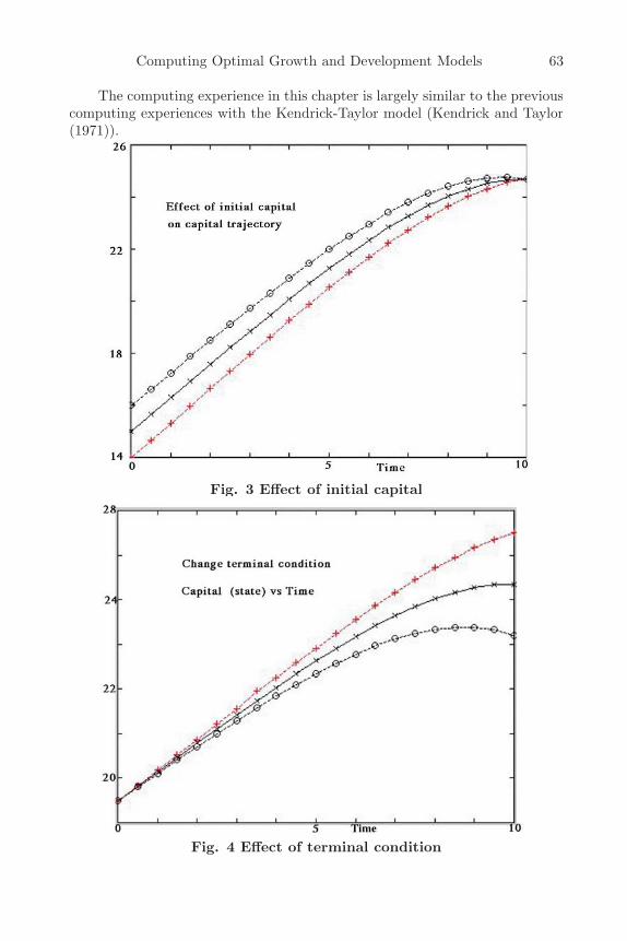
Computing Optimal Growth and Development Models 63
The computing experience in this chapter is largely similar to the previouscomputing experiences with the Kendrick-Taylor model (Kendrick and Taylor(1971)).
Fig. 3 Effect of initial capital
Fig. 4 Effect of terminal condition
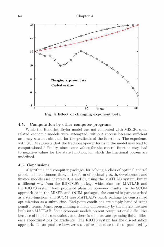
64 Chapter 4
Fig. 5 Effect of changing exponent beta
4.5. Computation by other computer programsWhile the Kendrick-Taylor model was not computed with MISER, some
related economic models were attempted, without success because sufficientaccuracy was not obtained for the gradients of the functions. The experiencewith SCOM suggests that the fractional-power terms in the model may lead tocomputational difficulty, since some values for the control function may leadto negative values for the state function, for which the fractional powers areundefined.
4.6. ConclusionsAlgorithms and computer packages for solving a class of optimal control
problems in continuous time, in the form of optimal growth, development andfinance models (see chapters 3, 4 and 5), using the MATLAB system, but ina different way from the RIOTS 95 package which also uses MATLAB andthe RIOTS system, have produced plausible economic results. In the SCOMapproach as in the MISER and OCIM packages, the control is parameterisedas a step-function, and SCOM uses MATLAB’s constr package for constrainedoptimization as a subroutine. End-point conditions are simply handled usingpenalty terms. Much programming is made unnecessary by the matrix featuresbuilt into MATLAB. Some economic models present computational difficultiesbecause of implicit constraints, and there is some advantage using finite differ-ence approximations for gradients. The RIOTS system has the discretisationapproach. It can produce however a set of results close to these produced by
Computing Optimal Growth and Development Models 65
the SCOM approach. While several computer packages are available for opti-mal control problems, they are not always suitable for a wide class of controlproblems. The MATLAB based RIOTS and SCOM, however, offer good op-portunities for computing continuous optimal-growth models. Optimal growthmodellers may find these algorithms and computer programs suitable to theirwork.
Chapter 5Modelling Financial Investment
with Growth5.1. Introduction
There are many models for financial investment, assuming that a pro-ductive economy is available to invest in. There are many economic models,commonly assuming that investment is a given quantity. However, questionsarise as to the mutual interaction of these two areas, especially the positive feed-back which may drive price changes. This chapter seeks to model some aspectsof this interaction, without assuming that the financial investors or plannersalways behave (or should behave) according to optimal economic principles.These models, like the other models in this book, assume new3 economics,and may be applied to social choice for an optimal intertemporal allocation offinancial and physical resources in the economy.
Should such a model be in discrete or continuous time? Models in con-tinuous time usually assume a Brownian motion as the basis of the stochasticcontribution, carrying with it a questionable assumption of independent contri-butions from non-overlapping time intervals, however short. A discrete- timemodel assumes less, and relates better to data which are available at discretetimes. Hence a discrete-time model is adopted here, including a stochasticincrement at each discrete time. If these increments are not too large, theresults can be adequately described by the evolution of the mean (or expecta-tion) and the variance. Thus, more complicated calculations about probabilitydistributions may be avoided.
When an objective function is to be maximized, for such a model, it isexpedient to approximate the dynamic difference equations for the mean andvariance by differential equations, in order to use available computer packagesfor optimal control. However, the results still relate to the discrete- time model.
The present approach makes some use of recent mathematics in optimiza-tion, which has been applied to some economic models (see e.g. Islam, 2001a;Chakravarty, 1979; Leonard and Long, 1992))
Some further discussion is given of multiple steady states in such dynamicmodels, and also of sensitivity questions, especially when the planning horizonis large, or infinite.
5.2. Some Related LiteratureThe essential elements of a dynamic optimisation model for investment
with growth (Islam, 2001a):i) the length of the planning horizon,
Modelling Financial Investment with Growth 67
ii) an optimization criterion,iii) the form of intertemporal time preference or discounting,iv) the structure of dynamic systems under modelling,iv) the initial and terminal conditions.There is extensive literature on methodology and practice for economic
areas such as optimal growth (see e.g. Islam, 2001a; Chakravarty, 1979), andon investment models (see e.g. Campbell and Viceira, 2002 for a recent account,also Karatzas, 1996 for modelling in continuous time, and dynamic optimisationmodelling in Taperio, 1998; Sengupta and Fanchon, 1997; Vickson and Ziemba,1975) ), some questions remain concerning the mutual interaction of these areas.
Dutta (1993) provides an up to date survey of results concerning the el-ements listed. The element (i) concerns the length of the planning horizon,the associated choice of a final period capital stock, and the possible choiceof an infinite horizon. Dutta (1993) cites some results of Brock (1997), Mitra(1983), and Mitra and Ray (1984), that establish, under some assumptionsincluding the continuity, convexity, etc. mentioned above, the insensitivityto horizon length, and the existence of a finite-horizon plan close to a giveninfinite-horizon plan. But this closeness does not always hold; there are counter-examples. Significant questions are whether a finite-horizon investment plan isrelatively insensitive to the exact choice of horizon length, and whether eachfinite-horizon optimal plan is close to some infinite-horizon optimum?
In (ii), optimization requires some objective function to be maximized (orminimized). Often, a utility function of consumption alone is chosen, usuallysatisfying properties of continuity, monotonicity, and concavity. However, itmay be appropriate to consider several objectives (see discussion in section 4b),and to relax the concavity requirement. Other optimality criteria, not oftenused for financial modelling include overtaking criterion, catching-up criterion,maximum criterion, etc. (Leonard and Long, 1992); there is some discussionin section 5.4.
For (iii), an infinite horizon generally requires some discount factor, butnot necessarily the usual exponential factor, since this assigns negligible value tothe far future. Alternative discount factors (see Heal 1998, Islam and Craven,2001b) may be considered, For (iv), terminal conditions are often given bytransversality conditions the value of the terminal year capital stock is specified,perhaps as zero (see Leonard and Long, 1998 for a survey).
The next paragraphs outline a number of specific financial models, dis-cussed in the literature. A recent discussion of computation of optimal port-folio choice problems may be seen in Islam and Oh (2003), and Oh and Islam(2001).
In more general financial models (see Sengupta and Fanchon 1997), thegrowth of wealth wt at times t = 0, 1, 2, . . . . is described by a dynamicequation wt+1 = rt(wt − ct), in which ct is consumption at time t, and rt is astochastic term, perhaps described by a first order Markov process. They usea logarithmic utility function, and maximize the present value:
∑ρtlog(ut).
68 Chapter 5
In the model of Hakansson (1975), there are M investment opportunitiesi = 1, 2, . . . , M. A dynamic equation, in discrete times t = 1, 2, . . . , relatescapital xt at the start of period t to the amount invested by:
xt+1 =∑
i
(βi − 1 − ρ)zit + (1 + ρ)(xt − ct) + yt ,
where ρ is interest rate (Hakansson’s quantity r = −1 + ρ);βi is the stochasticfactor which multiplies capital for investment i; yt = income from non-capitalsources; ct represents consumption; some assumptions are made on the βi . Anobjective function:
∑t
αtu(∑
i
((βi − 1 − ρ)zit(1 + ρ)(xt − ct) + yt =∑
t
αtu(xt+1)
is to be maximized, presumably with respect to variables zij . But it is notclear what bounds are placed on the zij ; and the costs of investment capi-tal are not explicit. Hakansson obtained an analytic optimum using dynamicprogramming.
The asset pricing model of Lucas (1978) was summarized in Judd (1998).In this model, a single asset pays dividends according to the ( AR(1) ) stochasticmodel yt+1 = ryt + et+1 , with independent identically distributed randomvariables et . The present value of utilities u(ct ) is maximized. The equilibriumprices pt satisfy:
u′(yt)pt = bE{u′(yt+1)(yt+1 + pt+1|pt},
where b is a discount factor. This leads to an integral equation for the pricespt . The dividends yt perhaps represent the consumption ct .
In another version of the model (see Gourieroux and Janiak, 2001), thepresent value of utility functions of consumption is maximized, subject to a“budget constraint”:
qtCtCC + atpt = Rt + at+1pt,
where qt denotes price of the (single) consumption good, at denotes a vector ofallocation of investment, CtCC denotes consumption, Rt denotes external income,pt is (presumably) the market price (vector) of the investments at time t. Anunconstrained optimum was sought, by setting the gradient to zero.
Malliaris and Brock (1982) describe Merton’s model, in which the shareprices are described by a stochastic process in continuous time. Consumptionand amount of new investment are decided by current prices. The objective tobe optimized is an integral of utility of consumption over the planning period,plus a function of wealth at the end time. All income is supposed to comefrom capital gains. A solution is obtained by stochastic dynamic program-ming. Malliaris and Brock also discuss an asset pricing model , based on Lucas
Modelling Financial Investment with Growth 69
(1978), which assumes the hypothesis of rational expectations (a hypothesis oninvestors’ behaviour), and involves stochastic terms. The existing dynamic fi-nancial models (including the ones discussed above) are not specified with anexplicit discussion of a set of the elements of a dynamic economic model. Theabove set of elements are chosen on an ad hoc basis in the existing literature.
5.3. Some ApproachesFor such stochastic models in continuous time, dynamic programming is
a useful theoretical technique, but it presents difficulties for numerical compu-tation. From a methodological viewpoint, a computation would require dis-cretization of both time and levels of prices, and arguably one might as wellstart with a discrete model. However, it may be questioned whether investors,or markets, indeed behave rationally according to Lucas’s model, or any other.Moreover, the growth factors, such as Hakansson’s βi , are extrinsic to themodels, and are thus not analysed. But growth rate should depend on physicalcapital, as discussed below in section 5.4, and investment, and so may be morespecifically modeled. A distinction is necessary between physical capital andits current (and fluctuating) market value.
These dynamic models have an inherent multiobjective character. Onemay wish to maximize both consumption and capital growth, both for the nearfuture and the more distant future. These objectives are in conflict, and animprovement on one may not compensate for a deterioration in another. Amodel may include several parameters, specifying the relative weight givento the conflicting factors, Thus, for example, a model could maximize thecapital at a horizon time, plus a proportion σ1 of an estimated future growth,subject to a floor on consumption, thus consumption ≥ σ2 at all times. Theresult of varying the parameters σ1 and σ2 would then need study, usuallycomputationally.
Suppose there are objective functions fiff (z) (i = 1, 2, . . .) to be maximized,subject to constraints gj(z) ≥ 0 (j = 1, 2, . . . ,m). Some of the fjf could be end-point terms, describing the far-future. As well as a Pareto maximum problemfor the vector objective f = (f1, f2ff , . . . .), other versions of the problem wouldturn one or more objectives into constraints, such as fjff (z) ≥ σj . (For thepresent, the parameter σj is absorbed into fjf , so fjf (z) ≥ 0 is written). For allof these related problems, the Lagrangian:
L =∑
τiττ fiff (z) +∑
λjgj (z)
is the same, and the Karush-Kuhn-Tucker (KKT) necessary conditions for anoptimum at z = p are the same, except that the multipliers τiττ and λj may takedifferent values. If hypotheses are assumed that make the KKT conditions alsosufficient for an optimum, then all of these problems are optimized at differentPareto points of the Pareto maximum problem for f . The hypotheses could bethat all the −fiff and −gj are invex with respect to the same scale function, or

70 Chapter 5
that all the fiff and gj are pseudoconcave . Equivalently, the vector function Q,whose components are all the −fiff and −gj , is invex if, for all x and p:
Q(x) − Q(p) ≥ Q′(p)η(x, p)
for some scale function η. Convexity is the case where η(x, p) = x − p. How-ever, invexity is enough to ensure that the necessary KKT conditions are alsosufficient for an optimum (see e.g. Craven, 1998).
However, invex may be difficult to verify for an optimal control problem,because the dynamic equation, an equality constraint, presents difficulties (seeCraven, 1998).
5.4.1. A proposed model for interqction between financial invest-ment and physical capital
An increase in share price does not directly increase productivity. Indi-rectly (and after some time delay) it may do so, by allowing additional capitalto be raised by a share or bond issue. The present model considers produc-tivity to depend on the physical capital (which is unchanged by a fluctuationin share price), plus additional investment, which may be explicitly modelled.The latter are of two general kinds, namely internal investment (that part ofthe profits which is used to increase physical capital, including raw materials,etc.), and external investment (from share issues, etc.)
How does physical capital affect the share price, and how does the shareprice affect external investment . If these aspects are to be modelled (insteadof putting some unexamined growth factor into the model), then some assump-tions must be made. Some simple assumptions are the following. The shareprice could be assumed to follow a random walk, say jumping up or down byan amount d with probability q for each jump, with d and q adjusted to matchan observed variance of share price. But the share price should tend to increasesomewhat with an increase (or positive rate of increase) of the physical capital.Perhaps the probability of jumping up by d should depend on the physical cap-ital? The external investment , it could be assumed to increase as share priceincreases (or perhaps when its rate of increase gets over a threshold?) Notethat this is a positive feedback path, hence tending to instability, and unlikelyto follow a linear law. These actual phenomena seem to fall outside the usualmarket model assumptions, but they may still be modelled.
Consider investment opportunities j = 0, 1, . . . , n, where j = 0 is ”risk-free” (i.e. a bank account, whose balance may be positive or negative). At timet = 0, 1, 2, . . . , T, let ktj = physical capital (measured by historical investment,in constant dollars); let mtj =market price; so “wealth” consists of terms mtjktj
. Instead of assuming an exogenous growth term, growth will be modelled, by:
kt+1,j = (1 − d)[ktj + g(bktj − ctj + ytj ],
where ctj = consumption (or sales, exports, etc.), ytj denotes new investment(e.g. from a share issue), g is an increasing concave function, describing a law

Modelling Financial Investment with Growth 71
of diminishing returns, d is a depreciation factor, and b(< 1) describes thefraction of capital that is available for growth. (This model is crude, sincephysical capital is of several kinds.)
The wealth at time t consists of terms mtjktj . Fluctuations in the marketprices mtj do not directly change the physical capital, on which growth de-pends, but they will affect the investment term ytj (which requires modellingin terms of the increase in wealth at a somewhat earlier time). The function gis analogous to the concave utility functions used by other authors, but is hereapplied to the capital available for growth. The bank account (j = 0) allows foradditional investment (subject to paying interest), or for selling assets withoutreinvesting them. If ztj units of investment j are held at time t, and vtj arepurchased during the period (t, t + 1) (with vtj < 0 for a sale), then:
vt0 + mt1vt1 + . . . + mtnvtn = 0 ;
zt+1,j = ztj + vtj (j = 1, 2, . . . , n);
zt+1,0 = [zt0 + mt1qt1 + . . . + mtnqtn ]
Here qtj describes any dividend or interest, or repayment of a bond.Consider first a simple model for market prices:
mt+1,i = mt,i + et,i + ζ[kt,i − kt−1,i],
in which the mt,i(t = 0, 1, 2, . . . ) are independent identically distributed ran-dom variables with a given variance σ2, and ζ is a small positive constant.Thus, the price is modelled as a random walk, with an additional small feed-back term depending on the change of physical capital. This feedback mayproduce instability − but note that market prices are, in fact, often unstable.The different investments j are considered here as independent, though thisassumption may need modification.
The new investment term ytj may be modelled as:
ytj = ζ ′[mtjktj − mt−1,jkt−1,j ]+ ,
where ζ ′ is a small parameter, and [w]+ := w if w ≥ 0, 0 if w < 0. Note thatthe time lag, here one interval, is another parameter that may be changed.
As well as this dynamic model, appropriate objective function and con-straints must be specified. One specification is to maximize the expectation ofthe wealth at the horizon time T :
E∑
j
mTjkTj ,
subject to a constraint on consumption:
ctj ≥ bj + b′jt (t = 0, 1, . . . , T ; j = 1, 2, . . . , n) .
72 Chapter 5
There might also be a cost term∑
t,j µ[c∗−ctj ] subtracted from the objective, todescribe a penalty cost imposed when the consumption is allowed to fall belowsome target level c∗. This formulation assumes that the far future (after timeT ) is accounted for by maximizing the wealth at time T . For each investmentj, there is a floor under consumption, which increases with time, at a rate givenby the parameters b′j .
Another specification maximizes a consumption objective:∑
j
rtU(ctj) +∑
j
σ1jU(cjT )rT /(1 − r) ,
in which U(.) is a (concave increasing) utility function, subject to the abovefloor on consumption, and to a terminal constraint on wealth:
E∑
j
mTjkTj ≥ σ3.
Here the parameters σ1j relate to the balance between short term and far-future, and σ3 relates to the balance between consumption and capital.
For the discrete-time optimal-control financial models considered here, theexistence of an optimum is automatic, since the feasible region is bounded, andcontinuous functions are involved. This existence result does not hold for acontinuous-time optimal control financial model, since infinite dimensions areinvolved. However, if the necessary Pontryagin conditions are solvable (as isthe case for all the continuous-time models considered in this chapter), thenthat solution is the optimum if either the solution is unique, or if a generalized-convexity condition such as invexity (see section 3b) holds as in many modelsof finance (and also economic growth), but uniqueness does not generally hold.
5.5. A computed model with small stochastic termIn this section, a financial model is developed and implemented, incorpo-
rating explicit relations between physical and financial capital, and so allowsthe extent of dependence of these two to be analysed.
For discrete time t = 0, 1, 2, . . . , denote kt = physical capital, ct = con-sumption, qt = external investment, c∗ = consumption target, mt = marketprice for shares, ρ = depreciation rate, and ϕ(s) = a(1− e−bs) is a concave in-creasing growth function. Consider the following dynamic equations for physicalcapital (which may include knowledge and human capital) and market price:
∆kt = −ρkt + ϕ(kt − ct + qt), k0 given
∆mt = θmt + µ∆kt + ξt, m0 given.
Here the coefficients θ, and µ > 0, describe a market price trend and an in-fluence of observed physical capital on market price; the ξt are i.i.d. randomvariables with mean zero. (A more complicated, Markovian, model could also
Modelling Financial Investment with Growth 73
be considered.) In particular, if the random terms are negligible and if θ = 0,then:
mt = m0 + µ(kt − k0).
The interaction between financial capital, namely the market value mtkt, andexternal investment qt is assumed to have the form qt = ε[∆(mt−1kt−1)]+ .Here ε is a small positive coefficient, and [.]+ makes only increases in marketvalue have an effect. There is a time lag, here of one unit. (This model doesnot discuss speculative investment.) Denote the expectation kt := Ekt, alsoyt := kt − kt , and mt := Emt.
Substitution of qt into the equation for ∆kt gives:
kt+1 = (1 − ρ)kt + ϕ(kt − ct + ε[∆(mt−1kt−1)]+).
The contribution of yt to the right side of this equation contains linear terms,whose expectation is 0, and a quadratic term, approximated by 1
2ϕ”(kt −ct)θ3mty
2t . Hence, denoting νt := sgn∆(mt−1kt−1 ) ,
kt+1 ≈ (1 − ρ)kt + ϕ(kt − ct + ε[∆(mt−1kt−1)]+)
+12εϕ”(kt − ct)mtνt var kt,
Approximating the contribution to yt+1 from ξt by the linear term
(1 − ρ)ξt + ϕ′(kt − ct)(ξt + εktξt−1)
gives:
varkt+1 ≈ (1 − ρ + ϕ′(kt − ct)) var kt + νt[εϕ′(kt − ct)kt]2 var mt.
These approximations may be appropriate when ε is small.The interactions described by µ (effect of physical capital on market price)
and ε (effect of market price on external investment) represent a feedback pro-cess, whereby an increase of physical capital tends to produce a further suchincrease.
The objective function to be maximized is taken as:
kT+1 − ωT∑
t=0
[c∗ − ct]2,
The elements of this model are (i) the finite planning horizon T, (ii) the ob-jective function, a utility function involving terminal capital and consumption,with a penalty when consumption falls too low (ω is a weighting factor), and(iii) boundary conditions, as upper and lower bounds on consumption.
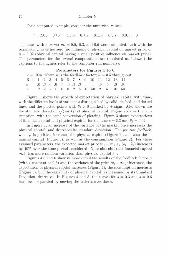
74 Chapter 5
For a computed example, consider the numerical values:
T = 20, ρ = 0.1, a = 4.0, b = 0.1, c = 0.4, ω = 0.5, ε = 3.0, θ = 0.
The cases with s := var mt = 0.0, 0.3, and 0.6 were computed, each with theparameter µ as either zero (no influence of physical capital on market price, orµ = 0.02 (physical capital having a small positive influence on market price).The parameters for the several computations are tabulated as follows (ıthecaptions to the figures refer to the computer run numbers):
Parameters for Figures 1 to 6κ = 100µ, where µ is the feedback factor; ω = 0.5 throughout.Run 1 2 3 4 5 6 7 8 9 10 11 12 13 14s .0 .3 .6 .0 .3 .6 .3 .3 .3 .3 .6 .6 .6 .6κ 2 2 2 0 0 0 2 5 10 50 2 5 10 50
Figure 1 shows the growth of expectation of physical capital with time,with the different levels of variance s distinguished by solid, dashed, and dottedlines, and the plotted points with θ2 > 0 marked by + signs. Also shown arethe standard deviation
√(var kt) of physical capital. Figure 2 shows the con-
sumption, with the same convention of plotting. Figure 3 shows expectationsof financial capital and physical capital, for the case s = 0.3 and θ2 = 0.02.
In Figure 1, an increase of the variance of the market price increases thephysical capital, and decreases its standard deviation. The positive feedback,when µ is positive, increases the physical capital (Figure 1), and also the fi-nancial capital (Figure 3), as well as the consumption (Figure 2). For theseassumed parameters, the expected market price mt = m0 +µ(kt−k0) increasesby 40% over the time period considered. Note also also that financial capitalmtkt has more random variation than physical capital kt .
Figures 4,5 and 6 show in more detail the results of the feedback factor µ(with ε constant at 0.3) and the variance of the price mt . As µ increases, theexpectation of physical capital increases (Figure 4), the consumption increases(Figure 5), but the variability of physical capital, as measured by its StandardDeviation, decreases. In Figures 4 and 5, the curves for s = 0.3 and s = 0.6have been separated by moving the latter curves down.
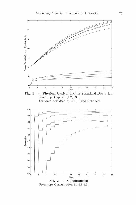
Modelling Financial Investment with Growth 75
Fig. 1 - Physical Capital and its Standard DeviationFrom top: Capital 1,4,2,5,3,6.Standard deviation 6,3,5,2 ; 1 and 4 are zero.
Fig. 2 - ConsumptionFrom top: Consumption 4,1,2,5,3,6.
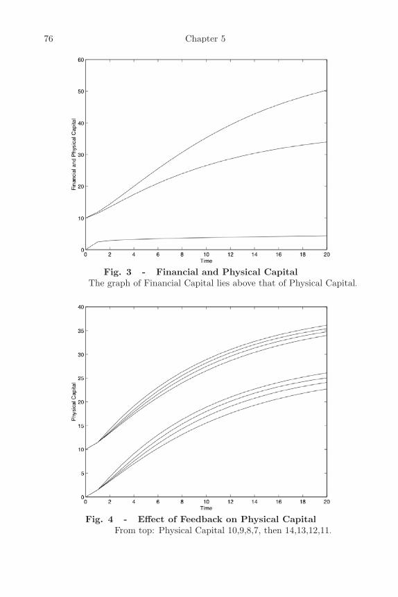
76 Chapter 5
Fig. 3 - Financial and Physical CapitalThe graph of Financial Capital lies above that of Physical Capital.
Fig. 4 - Effect of Feedback on Physical CapitalFrom top: Physical Capital 10,9,8,7, then 14,13,12,11.

Modelling Financial Investment with Growth 77
Fig. 5 - Effect of Feedback on ConsumptionFrom top: Consumption 14, 13, 12, 11, then 10, 9, 8, 7 with 0.1 subtracted.
Fig. 6 - Effect of Feedback on Variability of CapitalFrom top: Standard Deviations 11, 12, 13, 14,then 7, 8, 9, 10 with 1.0 subtracted.
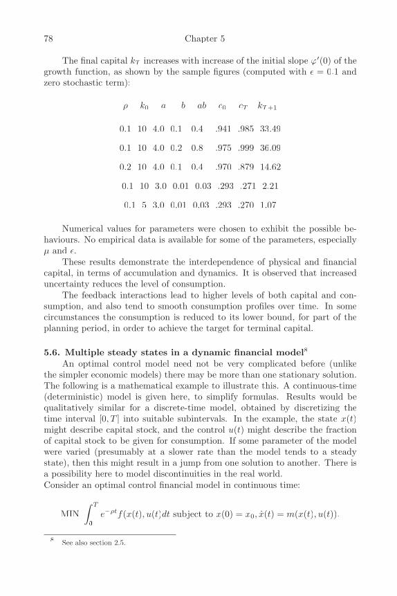
78 Chapter 5
The final capital kT increases with increase of the initial slope ϕ′(0) of thegrowth function, as shown by the sample figures (computed with ε = 0.1 andzero stochastic term):
ρ k0 a b ab c0 cT kT+1
0.1 10 4.0 0.1 0.4 .941 .985 33.49
0.1 10 4.0 0.2 0.8 .975 .999 36.09
0.2 10 4.0 0.1 0.4 .970 .879 14.62
0.1 10 3.0 0.01 0.03 .293 .271 2.21
0.1 5 3.0 0.01 0.03 .293 .270 1.07
Numerical values for parameters were chosen to exhibit the possible be-haviours. No empirical data is available for some of the parameters, especiallyµ and ε.
These results demonstrate the interdependence of physical and financialcapital, in terms of accumulation and dynamics. It is observed that increaseduncertainty reduces the level of consumption.
The feedback interactions lead to higher levels of both capital and con-sumption, and also tend to smooth consumption profiles over time. In somecircumstances the consumption is reduced to its lower bound, for part of theplanning period, in order to achieve the target for terminal capital.
5.6. Multiple steady states in a dynamic financial model8
An optimal control model need not be very complicated before (unlikethe simpler economic models) there may be more than one stationary solution.The following is a mathematical example to illustrate this. A continuous-time(deterministic) model is given here, to simplify formulas. Results would bequalitatively similar for a discrete-time model, obtained by discretizing thetime interval [0, T ] into suitable subintervals. In the example, the state x(t)might describe capital stock, and the control u(t) might describe the fractionof capital stock to be given for consumption. If some parameter of the modelwere varied (presumably at a slower rate than the model tends to a steadystate), then this might result in a jump from one solution to another. There isa possibility here to model discontinuities in the real world.Consider an optimal control financial model in continuous time:
MIN∫ T
0
∫∫e−ρtf(x(t), u(t)dt subject to x(0) = x0, x(t) = m(x(t), u(t)).
8 See also section 2.5.
Modelling Financial Investment with Growth 79
As with various economic growth models, no active constraints are assumedfor the control u(t). The time horizon T is assumed to be fairly large. But thediscount factor e−ρt prevents a steady state being reached. The Hamiltonianis e−ρtf(x(t), u(t))+λ(t)m(x(t), u(t). In terms of the steady state Hamiltonianf(x(t), u(t)) + Λ(t)m(x(t), u(t)), where Λ(t) = eρtλ(t), the adjoint differentialequation becomes:
−Λ(t) = fxff (x(t), u(t)) + Λ(t)mx(x(t), u(t)) − ρΛ(t)
(with no boundary condition), and Pontryagin’s principle (in the absence ofactive control constraints) requires that fuff (x(t), u(t))+Λ(t)mu(x(t), u(t)) = 0.A steady state, in which x(t), u(t) and Λ(t) take constant values, may be soughtby equating x(t) and Λ(t) to 0.
Can fairly simple functions f and m give rise to multiple steady states?Consider, in particular, m(x, u) = Φ(x)− ux, where Φ is a cubic, say Φ(x) =a + (3/2)x2 − x3 (assuming some scaling for x). Then Φ(x) − ux = 0 when a−ux + (3/2)x2 − x3 = 0, and this cubic will have three real roots x = x(u), foran interval of values of u, In particular, if a = 0, then:
x(u) = 0 or (1/2)(3 ±√
(9 − 16u)), with u < 9/16.
Consider, in particular,
f(x, u) = (1/2)(x2 + u2).
Then the steady state (if it exists) requires that:
Φ(x) − ux = 0;x + Λ(Φ′(x) − u − ρ) = 0;u + Λ(−x) = 0.
Hence x depends on u as discussed above, Λ = u/x, and
0 = x + (u/x)(3x − 3x2 − u − ρ) = 0.
Hence x must satisfy the equation:
0 = x2 + (Φ(x)/x)(3x − 3x2 − ρ) − Φ(x)2/x.
If, in particular, a = 0, and ρ = 0 (no discounting), then x satisfies a cubicequation, so that x = 0 or x satisfies:
1 + (3/2 − x)(3 − 3x) − x(3/2 − x)2 = 0.
Another instance of multiple steady states is given in Islam and Craven (2001).
80 Chapter 5
5.7. Sensitivity questions, concerning infinite horizonsConsider first a single-objective financial optimization problem:
MAXzF (z, q)) subject to g(z, q) ≤ 0, k(z, q) = 0,
where q is a perturbation parameter, and suppose that, when q = 0, a strictmaximum is reached at z = z(0). This means that, for small enough r > 0 :
[g(z, 0) ≤ 0, k(z, 0) = 0, ‖q‖ = r ] ⇒ F (z) ≤ F (¯(0)) − δ(r)
for some δ(r) > 0. Given also a continuity condition,, the strict maximumimplies that, for sufficiently small ‖q‖ , the perturbed problem reaches a localmaximum at ¯(q) close to ¯(0), thus ¯(q) → z(0) as q → 0. Clearly, this doesnot usually happen for a maximum that is not strict,
The additional conditions required for this result (see Craven, 1994) arethat (F, g, k) is uniformly continuous in a local region around the point (z, q) =(¯(0), 0), there are feasible solutions to the perturbed constraints, and, whenq = 0 , F (., q) reaches a minimum on each closed bounded set (this last wouldusually be assumed on economic grounds).
For an optimal control problem with state x(t) and control u(t), the dy-namic equation:
x(0) = x0 , x(t) = m(x(t), u(t), t) (t ≥ 0)
is assumed to determine x(.) as a function of u(.). So an objective function:
∫ T
0
∫∫f(x(t), u(t), t)dt + Φ(x(T ))
may be expressed as J(u(.)), to be maximized subject to constraints on u(.).The horizon T will be written as 1/q, where the perturbation parameter q = 0for an infinite horizon.
The uniform continuity condition is then not automatic. It is fulfilled (seesection 5.10) if f is quadratic, and high-frequency oscillations of the controlu(t) are suitably small.
Assume now that an optimum is reached at z(t) ≡ (x(t), u(t) = p(t).Several cases arise for the infinite horizon.
Case J(p) finite. This is only likely if f includes a discount term. If z(t)tends to a limit, q say, as t tends to infinity, f(q) will sometimes (dependingon the rate of convergence) be the dominating factor in J(p). Under some(substantial) boundedness conditions, a suitable time transformation t = k(s)(with k(.) increasing and k(0) = 0) maps the infinite time interval to [0,1], butmay produce an unbounded integrand. If f(z(t), t) tends fast enough to zeroas t → ∞, an equivalent control problem is obtained, over a finite interval oftransformed time s, and the Pontryagin theory applies to it. If the maximumfor the infinite horizon is strict, and the uniform continuity condition holds,

Modelling Financial Investment with Growth 81
then the optimum objective for horizon T will be close to the optimal objectivefor infinite horizon, provided that T is sufficiently large.
Periodic case. For some finite T, impose the boundary condition thatz(T ) = z(0). Assume no discount factor. Then the problem may be optimizedover [0, T], then it effectively starts again at t = T for a new interval [T, 2T ],and so on.
Case J(p) infinite, other than the periodic case. Since maximizing J(z) isnow meaningless, suppose that T−1
∫ T
0
∫∫f(z(t), t)dt → b as T → ∞ , and then
seek to maximize b(z). Can one maximize Q(T ) := T−1∫ T
0
∫∫f(z(t), t)dt for some
large enough fixed T, and derive from this some approximation to the requiredmaximum b? For this purpose, assume that the given problem reaches a strictmaximum of b∗ at z = p. Assuming also the uniform continuity condition, then1/T may be regarded as a perturbation parameter, applied to Q(T ) instead ofJ(T ), leading to a maximum of Q(T ) at some point p(T ) close to p∗.
Catching up criterion. Under this criterion, p(t) = (x(t), u(t)) is optimumif:
limsupT→∞
∫ T
0
∫∫[f(z(t), t) − f(p(t), t)]dt ≤ 0,
for feasible plans (x(t), u(t)). Equivalently, T−1∫ T
0
∫∫f(z(t), t)dt may be dis-
cussed, though a limit as T → ∞ is not necessarily assumed.However, the question of how large T must be, in order to closely approx-
imate the infinite horizon case, calls for further study.While these sensitivity results are stated for continuous-time optimal con-
trol models, the ideas also apply to discrete-time control models, such as thedynamic model of section 5.5 with a consumption objective.
5.8. Some conclusionsDynamic optimization models in finance can be usefully extended in several
directions, leading to a more integrated and operational approach. The aspectsconsidered include a systematic analysis of the elements of the model, the roleof physical capital, as distinct from fluctuating market value, some attempts tomodel investment, sensitivity to time horizons, possible multiple steady states,and some numerical calculations. A dynamic optimization model requires aspecification of a standard set of elements for a growth model.
While an infinite time horizon may not be thought relevant to financialmodelling, a long horizon may be, when a continuing enterprise is considered.Computation of a simple model, showing the interaction between physical cap-ital, financial capital, and investment, have led to several qualitative conclu-sions, detailed above.
Some issues remaining are to relate the model to empirical data, and toexplore the relevance of mathematical concepts such as generalized convexity(particularly invexity ) to these financial models.
A financial model of a different kind is the model by Davis and Elzinga
82 Chapter 5
(1972) for dividends and investment in a utility company. A computation ofthis model using the SCOM package is given in section 3.7; a stochastic versionis considered in Craven (2002).
The usefulness of MATLAB packages for such computations is not speed,but rather a great facility in changing model details and parameters, with-out needing extensive programming. The step-function approximations usedhere have been shown to be adequate, both theoretically (Craven, 1995) andcomputationally (Teo, Goh and Wang, 1990).
5.9. The MATLAB codesThese are the MATLAB codes used for the discrete-time optimal control
mode, including a small stochastic contribution. For purpose of computation,the difference equations have been approximated by differential equations, en-abling continuous-time optimal control software to be used.
The time scale: t = 0, 1, 2, . . . , n translates to t = 1, 2, . . . , nn + 1 inMATLAB M-code. The MATLAB package constr is called to optimize, giventhe functions from the following subroutines. The endpoint condition on thestate (capital) is computed as a penalty term. The parameters ω and µ in themodel appear in these codes as mu and fb respectively.
% fqs run.m % Calling programsubs=cell(1,9);subs={’fqsx’,’fqj’,’fqf’,’fqc’};par=[4, 1, 20, 0,0 ,20, 0.1, 3.0, 4.0, 0.1, 0.4, 0.5, 0.6, 1, 0.02];% nx nu nn 0 0 T rho eps a b c omega s switch mu% nx = n umber of states, nu = number of controls, nn = number of% intervalsnn=par(3); nu=par(2); nx=par(1);xinit=[10.0, 10.0, 0.0, 0.0]; % Initial conditions for statesu0=0.2*ones(nn,nu); ul=0.2*ones(nn,nu);%ul=zeros(nn,nu);uu=10*ones(nn,nu);Control=constr(’fqd’,u0,[],ul,uu,[],par,subs,xinit)[jf,g,state]=feval(’fqd’,Control,par,subs,xinit);statejfy1=Control; y2=state(:,1); y3=sqrt(state(:,4));
function [f,g,state] = fqd(um, par, subs, xinit) % Organize computationnx=par(1); nu=par(2); nn=par(3);b=par(6);ıpd=char(subs(1));xm=zeros(nn+1,nx); xm(1,3a)=xinit;´for tc=1 : nnff=feval(pd,tc,um,xm,par);xm(tc+1,3a) = xm(tc,:) + ff;´
Modelling Financial Investment with Growth 83
end% compute objective functionjf=0; pd=char(subs(2));for tc=1 : nnff=feval(pd,tc,um,xm,par);jf=jf+ff;endpd=char(subs(3));jf=jf+feval(pd,tc,um,xm,par);pd=char(subs(4));for tc=13anng(tc)=feval(pd,tc,um,xm,par);endf=jf;state=xm;
function ff=fqsx(t,um,xm,par) % RHS of dynamic equationsnn=par(3);T=par(6); hh=T/nn; cc=par(11);mu=par(12); fb=par(15);del=par(7);eps=par(8);aa=par(9);bb=par(10);sig2=par(13);mt=1.0+fb*(xm(t,1)-xm(1,1));mm=mt+fb*xm(t,2);temp=xm(t,1)-um(t,1)+eps*mm*max(xm(t,1)-xm(t,2),0);swit=par(14);ph1=aa*bb*exp(-bb*temp);ph2=-bb*ph1;temp2=eps*ph1*xm(t,1);ff(1)=(-del)*xm(t,1)-aa*(exp(-bb*temp)-1)
+swit*eps*mt*ph2*xm(t,4); % Capitalff(2)=xm(t,1)-xm(t,2); % Relates to differences of Capitalff(3)=max(cc-um(t,1),0)2; cc-um(t,1);ff(4)=(-del+ph1)*(-del+ph1)*xm(t,4)+swit*temp2* temp2*sig2;
function ff=fqj(t,um,xm,par) % Objective integrandnn=par(3);T=par(6); hh=T/nn; cc=par(11);del=par(7);eps=par(8);aa=par(9);bb=par(10);ff=0;
function ff=fqf(t,um,xm,par) % Objective endpoint termnn=par(3);T=par(6); hh=T/nn; cc=par(11);del=par(7);eps=par(8);aa=par(9);bb=par(10);mu=par(12);ff=-xm(nn+1,1)+mu*xm(nn+1,3);xm(nn+1,3);
5.10. Continuity requirement for stabilityFor a control problem on an infinite time domain, assume that the control u(t)satisfies ‖u‖2 = [
∫ ∞0
∫∫ |u(t)|2dt < ∞. Denote by Qu(s) the Fourier transform of
84 Chapter 5
u(.). Now assume, more restrictively, that ‖b(.)Qu(.)‖2 is finite, for a regionaround the optimal u(.), where the weighting function b(s) is positive, andb(s) → ∞ as s → ∞. This places a serious restriction on high-frequency oscil-lations of u(t). Assuming this, the uniform continuity requirement for the sen-sitivity result follows for functions f which are linear or quadratic (see Craven,1994), and hence for some other functions whose growth rate is no more rapidthan these.
Chapter 6Modelling Sustainable Development6.1. Introduction
The issues of sustainability of growth, and social welfare that ensures in-tergenerational equity, are controversial, and form an important area of studyin social welfare and social choice in contemporary models. In recent litera-ture, Hamiltonian-based measures of social welfare have been used to definethe concept of sustainable growth In the mainstream economic interpretation,where social welfare is measured in terms of pure economic variables such asincome or consumption, sustainable growth relates to economic conditions ofnon-declining consumption or capital (whether man-made, natural, or environ-mental) over time. Sustainable growth has been formalised in different ways.In the optimal growth literature, sustainable consumption is characterized bythe golden age, representing the maximum consumption possible without re-ducing the potential for the same level of consumption in the future. Given thenumerical orientation of this study, the objective function here has cardinality,measurability and intergenerational utility and welfare comparability implica-tions. Several other definitions of sustainability have been given (Faucheux,Pearce and Proops, 1996). Conceptual and theoretical studies of sustainabil-ity are well advanced. In spite of several operational numerical studies of thisissue (e.g. Islam, 2001a), there is still a strong need for operational methodsfor sustainability modelling. This chapter presents several operational modelsand methods for sustainable growth and welfare, in order to explore a range ofoptimal control models in welfare economics.
6.2. Welfare measures and models for sustainability9
Various theoretical articles (Heal, 1998; Faucheux, Pearce and Proops,1996; Smulders, 1994) have incorporated sustainability in optimal growth mod-els. In terms of optimal control theory, sustainable consumption or welfare foran autonomous infinite-horizon problem have been described by a Hamiltonianfunction (see Leonard and Long, 1992; and Heal, 1998.)
Consider an infinite-horizon model, formulated as an optimal control modelfor social choice and optimal development:
V(a, b) := MAX∫ ∞
a
∫∫e−ρtf(x(t), u(t))dt subject to:
x(a) = b, x(t) = m(x(t), u(t)) .
Here x(t) is the state function (e.g. capital), u(t) is the control function (e.g.consumption), and u(t) is unconstrained. Denote by λ(t) the costate function,
9 See also section 2.1.
86 Chapter 6
and by Λ(t) = λ(t)eρτ the current-value costate function. The current-valueHamiltonian is:
h(x(t), u(t),Λ(t)) = f(x(t), u(t)) + Λ(t)m(x(t), u(t)).
Denote the optimal functions by x∗(t), u∗(t),Λ∗(t). Under some restrictions (seeSection 3.3), including the requirement (usually fulfilled) that λ(t) = O(e−βt)as t → ∞ for some β > 0, and no constraints on the control u(t), it may beshown that:
h(x∗(t), u∗(t),Λ ∗ (t)) = −ρV (t, x∗(t)) = −ρe−ρτV (0, x∗(t) → 0 as t → ∞.
The proofs in Weitzman (1976), Leonard and Long (1992) and Heal (1998) areincomplete, and do not state some necessary restrictions. Although the twofunctions:
h(x∗(t), u∗(t),Λ ∗ (t)) and δ−1
∫ ∞
t
∫∫f(x∗(τ), u∗(τ)e−δ(τ−t)dτ
satisfy the same first-order differential equation, their equality only follows ifthey satisfy a common boundary condition, namely both → 0 as t → ∞ , whichfollows from h(x∗(t), u∗(t),Λ ∗ (t)) → 0.
Weitzman (1976) and subsequent authors have interpreted V (t, x∗(t)) asthe stock of total wealth , and also h(x∗(t), u∗(t),Λ∗(t)) as the interest on totalwealth , which may be taken as a measure of sustainable income, utility orsocial welfare.
There are many criticisms of this approach to measurement of sustainablewelfare and sustainability (Arronsson, Johanssson and Lofgren, 1997,; Brekke,1997; Heal, 1998; and Land Economics, 1997). The Hamiltonian approach as-sumes very restrictive and unrealistic conditions, including (i) constant discountrate, technology, and terms of trade, (ii) time autonomous dynamic systemsin continuous time, (iii) no constraints on the control or state functions, (iv)positive social time preferences, and (v) convex optimal control models (so thatnecessary optimality conditions are also sufficient.) The assumption of a sin-gle capital good may not be necessary. Some aspects of this approach needmore attention, including transversality conditions, and conditions when theHamiltonian approaches zero for large times. Overtime and intercounting com-parisons are not possible; the consumption path has a single peak, and this isnot sustained; and the dictatorship of the present is embedded in the model. Ifnon-autonomous dynamics are considered, thus assuming x(t) = m(x(t), u(t), t)where m(.) depends explicitly on t, then x(t) and u(t) will not generally tend tolimits x(∞ ) and u(∞) as t tends to infinity; this is the case with the Kendrick-Taylor model considered in Section 5. For an autonomous model, the limits (ifthey exist) must satisfy 0 = m(x(∞), u(∞)).
Modelling Sustainable Development 87
Work on computational models and methods for sustainable growth isgenerally less advanced, although some simple approaches have been tried (seeCesar, 1992; Smulders, 1994; and the journal issue Land Economics, 1997).The object of the present chapter is to develop some mathematical and compu-tational models and methods for sustainable growth, within the framework ofwelfare economics (Arrow et al., 2003). They include the elements of an opti-mal growth program (Islam, 2001) such as an objective function, time horizon,time preference and terminal constraints.
There are several ways to embed sustainability into mathematical formula-tions of a computable optimal growth and development models. These includethe following:
(a) Including environmental factors and consequences in the model, e.g. bydynamic equations, or suitable constraints, for resource supply and exhaustion,pollution generation, etc. (see Heal, 1998; Cesar, 1994). See section 6.5.1.
(b) Appropriate specification of the objective function, to express the prin-ciples or criteria for sustainable growth (see section 6.3.1)
(c) Modelling intergenerational equity, reflected in social time preference,by suitably modified discount factors (see section 6.3.2)
(d) Considering a long-term planning horizon, or an infinite horizon in anoptimal growth model, so as give suitable weight to the long-term future, aswell as to the short-term, e.g. by Rawls (1972) or Chichilnisky (1977). (Seesections 6.3.2 and 6.3.3).
The chapter is structured as follows. In sections 6.3 and 6.4, some math-ematical models and methods are provided, for including sustainability in anoptimal growth model. The Kendrick-Taylor model is modified in Section 6.5to incorporate sustainability criteria. The results of computational experimentsare presented in Section 6.6. Conclusions and computational recommendationsare given in section 6.7.
6.3. Modelling sustainability
6.3.1. Description by objective function with parametersSustainability should be studied within a social choice framework. The
present discussion assumes the possibility of a social choice by a social welfarefunction (objective function). This function may contain utilitarian and non-welfaristic elements of social choice. It must incorporate, in some suitableform, the concerns for sustainability. If a description using a single objective issought, that of Chichilnisky (1996) is as plausible as any available. It includesa parameter α, which must be chosen to set the balance between short-termand long-term. This objective function may be written:
α
∫ ∞
0
∫∫U(c(t), k(t), t)e−ρtdt + (1 − α)limt→∞U(c(t), k(t), t) ,
perhaps with some replacement for the discount factor (see Section 4.2). Thismodel assumes that limits exist (so excluding any oscillatory models,) and it is
88 Chapter 6
not computable as it stands, because of the infinite time range. As remarked inSection 2, the assumed limits as t → ∞ will normally require that the functionm in the dynamic equation, and also the utility U, do not depend explicitlyon t. Moreover, some bounds on the variables should be adjoined, (compareRawls, 1972,) and some lower bound on consumption (thus introducing a fur-ther parameter.) Note that capital k(t) and consumption rate c(t) are vectorfunctions − though scalar functions may be considered first to simplify the dis-cussion. Note that environmental factors may enter as components of capital;for example, if p(t) is some measure of environmental degradation, then −p(t)could be a component of k(t).
However, a model with a single objective may not represent importantaspects of the system being modelled. An alternative approach adjoins con-straints, containing parameters. For example, consider a growth model withconsumption u(t) and capital stock k(t), and with some floor specified for theconsumption. This may relate to a minimum consumption as a function oftime, or among various consumers. Some simple examples are as follows.
(a) MAXu,xΦ(x(T )) subject to (∀t)u(t) ≥ b1,
x(0) = x0, x(t) = m(x(t), u(t), t)(t ∈ [0, T ].
Here the parameter b describes the minimum consumption level allowed.
(b) MAXu,x,b b subject to (∀t)u(t) ≥ b1,
x(0) = x0, x(t) = m(x(t), u(t), t)(t ∈ [0, T ],Φ(x(T )) ≥ Φ0.
Minimum consumption is maximized, subject to a minimum level for the finalcapital. A simple special case, with x(t) ∈ R and u(t) ∈ R, is:
MAXu,x,b b subject to (∀t)u(t) ≥ b1,
x(0) = x0, x(t) = αx(t) − u(t)(t ∈ [0, T ], x(T ) ≥ xT ,
at which the optimum (supposing the constraints to be feasible) is evidently atu(.) = b1.
(c) Denoting Pareto maximum by PMAX, consider:
PMAXx,u,b {b,Φ(x, T ))} subject to (∀t) u(t) ≥ b, b ≥ b0,
x(0) = x0, x(t) = m(x(t), u(t), t)(t ∈ [0, T ] . Φ(x(T )) ≥ Φ0.
(d) A variant of (a) considers a bound on average consumption:
T−1
∫ T
0
∫∫c(t)dt ≥ b2

Modelling Sustainable Development 89
(with b2 > b1 in (a)). This constraint may be included as a penalty cost, byintroducing a new state variable y(t) :=
∫ t
0
∫∫T−1c(s)ds, and then the constraint
y(T ) ≥ b2 enters as a penalty cost of the form µ[−y(T ) + b3]+ added to thetotal cost to be minimized. (Here [.]+ replaces negative vector components byzeros, and b3 ≈ b2.)
Note that examples (a) and (b) will give single elements of the set of Paretomaxima. Several values of the parameter b might be considered, in order todiscuss a tradeoff between consumption and capital. A similar remark appliesto the parameter α in the Chichilnisky model.
Some other Pareto maxima may be obtained by maximizing a weightedcombination ωT
1 b + ω2Φ(T ) . While this is often proposed, some criterion forchoosing the weights would be required. It may be more meaningful to considera parameter such as b instead.
6.3.2. Modified discounting for long-term modellingA model must maintain a suitable balance between short-term and long-
term utility. Consider an optimal control model with a state x(.) (e.g. a capitalfunction) and a control u(.) (e.g. a consumption function), and a time horizonT, with an objective of the form:
∫ T
0
∫∫e−δtf(x(t), u(t))dt + Φ(x(T )).
A variant considers∫ ∞0
∫∫and limt→∞Φ(x(T ). The traditional discount factor
e−δt gives negligible value to the far future, so this is not a sustainable model.If the discount factor is omitted, then the model may not be comparable withmodels for alternative investment of resources, since it does not allow for pos-sible growth when profits are reinvested.
The e−δt discount factor assumes that money can be invested so as to growat a compound-interest rate eδt. But such real growth can only happen over afairly short time horizon, during which suitable investments may be available,perhaps with some limit on the amount invested. The continued exponentialgrowth shown in some datasets for longer time periods merely describes mon-etary inflation. A continued exponential growth in real terms will soon meetresource constraints (e.g. Forrester, 1971,) or social constraints (e.g. a financialcollapse). When a particular activity, or enterprise, is modelled, there is alwaysassumed some background of other activities (in the sector, industry, etc.), thatis not being described in detail, but rather in some aggregated way. Withouta background to invest money in, discounting has no meaning
A more realistic discount factor would not assume an indefinite real growth;instead, some saturation effect would appear. A better description is requiredfor background growth, meaning the growth available in the larger system, ofwhich the model being studied forms a part. If g(t) describes the backgroundgrowth, then a possible description is given by: g(t) = δg(t)/(1 + ρt)2. Thisgrowth starts as exponential, but later approaches saturation. For this growth

90 Chapter 6
rate, g(t) = g(0) exp(δt/(1 + ρt). Thus g(t)/g(0) → eδ/ρ as t → ∞; qualita-tively, saturation starts to matter at about time 1/ρ. The discount factor isthen σ(t) = 1/g(t). Of course, there are other functions than this one with thedesired qualitative properties. But, lacking numerical data on saturation, it isappropriate to choose a simple function.
Another possible description for background growth assumes a maximumlevel for capital, and a logistic function for its growth rate, thus:
g(t) = δg(t)[1 − βg(t)], g(0) = g0.
This integrates to:
g(t) = aeδt/[1 + βaeδt] where g0 = a/(1 + βa), a = g0/(1 − βg0).
Thus, as t → ∞, g(t) → 1/β, the assumed maximum level. This model may bemore plausible than the previous one where the saturation is a given functionof time t. The discount factor is then σ(t) := 1/g(t) = e−δt + βa . Thus ittends to a positive constant value for large times.
Heal (1998, page 98) considers a class of discount factors ∆(t) satisfying∆′(t)/∆(t) → 0 as t → ∞ , for which the term limt→∞Φ(x(T ) does not affectthe optimum. The classical exponential discount factor does not satisfy thiscondition; the modified discount factor 1/g(t)given above satisfies it. ThenHeal’s criterion is satisfied for both the functions σ (.) proposed here, since:
σ(t)/σ(t) = −δ/(1 + ρt) + δρ/(1 + ρt)2or − δ/(1 + βaeδt,
and each of these → 0 as t → ∞.The Strotz phenomenon (see Chakravarty 1969, page 41) shows that only
with an exponential discount factor can a certain balance be achieved betweenan optimum path starting at time 0 and an optimum path starting at a latertime. Unfortunately this is incompatible with giving proper weight to the moredistant future.
6.3.3. Infinite horizon model10
Optimal control models of the form:
MINu(.),x(.)F (x, u) :=∫ ∞
0
∫∫e−ρtf(x(t), u(t), t)dt subject to:
x(0) = x0, x(t) = m(x(t), u(t), t), a(t) ≤ u(t) ≤ b(t)(t ≥ 0),
have often been considered in recent economic literature (sometimes as MAXF (x, u) ⇔ MIN −F (x, u)), often without explicit bounds on the control u(t),and often with e−ρt as the only explicit dependence on t. However, for the
10 See also Section 2 2 and chapter 9.
Modelling Sustainable Development 91
infinite horizon, it may not be obvious whether a minimum, or maximum, isreached; and the Pontryagin theory of optimal control is commonly presentedonly for a finite time horizon, since some assumptions about uniform approxi-mation over the whole time domain are involved. For an infinite horizon, somefurther restrictions are required for validity. The present discussion assumeslimiting behaviour as t → ∞, which ensures that the infinite-horizon problemis closely approximated by a problem with finite horizon T. Consequently, anyweight attached to the distant future must be expressed by a separate term inthe objective, as e.g. in the Chichilnisky model.
Assume that a minimum is reached, at (x∗(t), u∗(t)). The discount factore−ρt is needed, so that F (x, u) is finite. Following the approach in Craven(1995), the differential equation with initial condition is expressed in abstractform as Dx = M(x, u); the Hamiltonian is:
h(x(t), u(t), t, λ(t) := e−ρtf(x(t), u(t), t) + λ(t)m(x(t), u(t), t),
and the integral of the Hamiltonian equals H(x, u, θ) := F (x, u) + θM(x, u),where θ is a Lagrange multiplier vector, and λ(t) is a function representing θ.
Assume that x∗(t), u∗(t), and λ ∗ (t) (from the adjoint equation below)tend to limits as t → ∞ , with λ∗ (t) = O(e−βt) as t → ∞; f(., ., .) and m(., ., .)are twice differentiable functions, such that the second derivatives:
fxxff (x(t), u(t), t),mxx(x(t), u(t), t), fxuff (x(t), u(t), t),mxu(x(t), u(t), t)
are bounded in t, whenever (x(t), u(t)) are near to (x∗(t), u∗(t)).Note that an oscillatory optimum control is thus excluded; and the expo-
nential decay terms mean that the infinite horizon is closely approximated byproblem over (0, T), for some suitable finite T.
The steps in the proof, based on (Craven, 1995) are as follows; only thesignificant changes for an infinite horizon need be detailed.
(a) Obtain first-order necessary conditions.
(b) From (a), deduce the adjoint differential equation:
−λ(t) = (∂/∂x)h(x(t), u(t), t, λ(t)) , λ(t) → 0 as t → ∞.
Here λ(t) is assumed to represent θ, subject to verification that the differentialequation obtained is solvable; the calculation using integration by parts is valid,under the assumptions on limits as t → ∞.
(c) A linear approximation:
H(x, u, θ) − H(x∗, u, θ) = HxH (x∗, u∗, θ∗)(x − x∗) + o(‖u − u∗‖)holds, given the bounded second derivatives, noting that a term e−ρt is presentin FxFF , and e−βt in θMxMM ; here ‖u − u∗‖ =
∫ ∞0
∫∫ |u(t) − u∗(t)|dt. The quasiminproperty follows:

92 Chapter 6
H(x, u∗, θ) − H(x∗, u∗, θ) ≥ o(‖u − u∗‖).
(d) Assume that control constraints, if present, are a constraint on u(t)for each time separately. If h(x∗(t), . , t, λ ∗ (t)) is not minimized at u∗(t)(possibly except for a set E of t for which
∫E
∫∫dt = 0), then a standard proof
(not depending on the domain of t) shows that the quasimin is contradicted.Suppose now that an endpoint term limT→∞v(x(T )) is added to the ob-
jective function. This has the effect of adding v(x(t))δ(t−T ) to f, then lettingT → ∞. In consequence, the boundary condition for the adjoint equation be-comes:
λ(t) − v′(x(t)) = O(e−βt) as t → ∞.
If x(t) tends to a limit as t → ∞ (which implicitly assumes that f and m do notexplicitly contain t), and v(.) is continuous, then the limit of v(x(T )) exists.This remark applies to the Chichilnisky criterion in Section 6.4.2.
6.4. Approaches that might be computed
6.4.1. Computing for a large time horizonAs discussed in Section 3.1, it is appropriate to discuss optimization models
with parameters − required to take account of the several conflicting objectivesthat exist − and the question of what happens to the optima when theseparameters are varied provides a further stage of exploration. However, themodel must be somewhat recast, in order that a computer package can handleit, whether RIOTS 95 (Schwarz, 1996) or any other. Assuming that the limitsas t → ∞ exist, a nonlinear time transformation t = ψ(τ) may be applied, soas to compress the time scale for large times t (when little is changing). Acomputation requires a discretization of the time interval into finitely manysubintervals, and such a transformation considerably reduces the number ofsubintervals required (see Craven, 1995).
6.4.2. The Chichilnisky criterion with a long time horizonIf a discount factor e−ρt is retained, then the Chichilnisky model may be
approximated, for some large T, by:
MAXα
∫ T
0
∫∫e−ρtU(c(t), k(t))dt + αU(c(T ), k(T ))ρ−1e−ρT
+(1 − α)V (k(T ))
subject to k(0) = k0; k(t) = m(c(t),
k(t)), cU ≥ c(t) ≤ cL(0 ≤ t ≤ T ); k(T ) ≥ kT .

Modelling Sustainable Development 93
The second term is an estimate of the contribution for times beyond T; asimilar estimate is the salvage value cited in (Chakravarty, 1969). The followingassumptions are made:
• the utility U(., .) and the dynamics function m(., .) have no explicitdependence on time t;
• T is assumed large enough that c(T ) and k(T ) approximate their limitsas → ∞ ;
• the term in e−ρt estimates the integral from T to ∞;
• the lower bound cL on consumption is assumed constant (achievable byscaling c(t);
• the upper bound cU is included to bound the region where an algorithmmust search;
• the utility V applicable at time T may, but need not, be the same as U .
Note that the utility V depends on the final capital k(T ), but not on thefinal consumption u(T ), since u(T ) is not of significance, but rather the wholecurve of consumption versus time.
The constraint k(∞) ≥ kT may be replaced by a penalty term:
12µ[k(∞) − kT + µ−1ε]2+ ,
where µ is a positive parameter, and [ ]+ replaces negative components by zero;ε ≥ 0 will be adjusted, so as to fulfil the constraint exactly. According to thetheory of augmented Lagrangians (see the discussion in Craven, 1978), ε relatesto a Lagrange multiplier. If c(t) does not meet its bounds, then the inactiveconstraints on c(.) can be omitted. According to the Pontryagin theory, withsome regularity assumptions because of the infinite domain (notably that thelimits exist), an optimum satisfies the differential equation for k(t), the adjointdifferential equation:
−λ(t) = −e−ρtUkU (c(t), k(t)) + λ(t)mk (c(t), k(t), t),
λ(∞) = µ[k(∞) − kT + µ−1ε]+ − (1 − A)VkVV (k(∞);
and (from the Pontryagin principle):
−αe−ρtUcUU (c(t), k(t)) + λ(t)mk(c(t), k(t), t)(0 ≤ t < T ).
The adjoint differential equation is required for computing the gradient of theobjective.
When T is large, and the only explicit time dependence is the discountfactor, it may be useful to transform the time scale nonlinearly by:
t = ψ(τ) := −ρ−1log(1 − βτ), where β = 1 − e−ρT ;
94 Chapter 6
this maps τ ∈ [0,1] to t ∈ [0, T]; dt/dτ = (β/ρ)(1−βτ)−1 = (β/ρ)eρt. Denotingu(τ) := c(ψ(τ)) and x(t) := k(ψ(τ)), the problem is transformed to:
MAXJ(u) := α
∫ 1
0
∫∫U(u(τ), x(τ))dτ + αU(u(1), x(1))ρ−1e−ρT
+(1 − α)V (u(1), x(1))
= α
∫ 1[
0
∫∫U(u(τ), x(τ)) + δ(τ − 1)W (u(τ), x(τ)]dτ
where W (u(τ), x(τ) := U(u(τ), x(τ)ρ−1e−ρT + α−1(1 − α)V (x(τ))
subject to: x(0) = k0;
x(τ) = (β/ρ)m(u(τ), x(τ), ψ(τ))/(1 − βτ)(0 ≤ t ≤ T ),
cU ≥ u(t) ≥ cL(0 ≤ τ ≤ 1); x(1) ≥ kT .
Here x(τ) means (d/dτ)x(τ).The adjoint differential equation is then:
−λ(t) = −αUxUU (u(τ).x(τ)) + (β/ρ)mx(u(τ), x(τ), ψ(τ))/(1 − βτ);
λ(1) = −(α/ρ)e−ρT UxUU (u(1), x(1)) − (1 − α)VxVV (u(1), x(1)) + µ[k(T ) − kT
+µ−1ε]+
The gradient of the objective is then computed (when z(1) = 0) from :
J ′(u)z = −α
∫ T
0
∫∫[UuUU (x(τ), u(τ)) + (β/ρ)λ(τ)mu(u(τ), x(τ))/(1 − βτ)]z(τ)dτ
6.4.3. Chichilnisky model compared with penalty term modelIn the approximated Chichilnisky model considered in Section 6.4.2, the
second term with e−ρT estimates∫ ∞
T
∫∫e−ρt U(c(t), k(t))dt, in the case when
c(T ) and k(T ) are close to limiting values. (For the Kendrick-Taylor modeldiscussed below in Section 5, there are no limiting values.) The comparison fora discount rate ρ = 0.03 and horizon T = 20 years):
∫ T
0
∫∫e−ρtdt = ρ−1(1 − e−ρT ) ≈ 0.55 with e−ρT ≈ 15.04
shows that the term is unimportant, if U and V are of comparable size.Neglecting it, the objective reduces to:
α{∫ T
0
∫∫e−ρtU(c(t), k(t))dt + α−1(1 − α)V (k(T ))}.
Modelling Sustainable Development 95
If k(.) has only one component, then a reasonable choice for V (k(T )) would be:
−ξ[k(T ) − k#]2 or − ξ[k(T ) − k∗]2+ ,
where µ is a suitable positive parameter. (Of course, another form thanquadratic could be chosen; the quadratic is convenient to compute). The twoversions describe attainment of a target, or perhaps exceeding it. Then theobjective becomes:
α{∫ T
0
∫∫e−ρtU(c(t), k(t))dt +
12µ[k(T ) − k#]2},
with µ = 2ξα−1)1 − α), and perhaps [ ] replaced by [ ]+.This may be compared with adding to the integral a penalty term, to
represent an endpoint constraint k(T ) = kT (or k(T ) ≥ kT ). The penalty termhas the same form, with k* differing a little from kT , the difference dependingon µ and on a Lagrange multiplier in the optimization. In fact, the SCOMpackage handles an endpoint constraint in exactly this way.
It follows that the modified Chichilnisky model may be studied as a para-metric problem, with µ and k* as parameters.
6.4.4. Pareto optimum and intergenerational equityIntergenerational equity (and also sustainability) can be interpreted in
terms of Pareto optimality. Consider now two objective functions, say:
F 1(x, u) :=∫ T
0
∫∫e−ρtf(x(t), u(t))dt and F 2)x, u) := Φ(x(T ))
to describe, in some sense, utilities for the present generation and a futuregeneration, where x(t) denotes rate of consumption, and k(t) denotes capital(both may be vectors). Assume that these functions are constrained by a dy-namic equation for (d/dt)x(t), and bounds on u(t). Suppose that (x∗, u∗) is aPareto maximum point of this model. Then (assuming some regularity of theconstraint system), Karush-Kuhn-Tucker necessary conditions, or equivalentPontryagin conditions, hold for (x∗, u∗) exactly when these conditions hold fora single objective function τ1F
1(.) + τ2ττ F 2(.) , for some nonnegative multipli-ers τ1, τ2ττ , not both zero. Different points in the (large) set of Pareto optimacorrespond to different choices of the multipliers. For the two-objective prob-lem, the costate becomes a matrix function Λ(t), and the Pontryagin maximumprinciple considers a Pareto maximum of a vector Hamiltonian:
(F 1(x, u), F 2(x, u)) + Λ(t)(RHS of dynamic equation )
with respect to u(t) (see Craven, 1999).This may be compared with the parametric version of Chichilnisky’s cri-
terion:
αF 1(x, u) + (1 − α)F 2(x, u) = α[F 1(x, u) + βF 2(x, u)], β = α−1(1 − α).
96 Chapter 6
Each choice of α, or β, gives a different Pareto maximum point.
6.4.5. Computing with a modified discount factorIf the discount factor is modified to e−ρt + κ , then integration over an
infinite time domain will give infinite values. Instead, the following model maybe considered:
MAX α
∫ T
0
∫∫[e−ρt + κ]U(c(t), k(t))dt + (1 − α)V (k(T ))
subject to k(0) = k0; k(t) = m(c(t), k(t), t), cU ≥ c(t) ≥ cL(0 ≤ t ≤ T );k(T ) ≥kT .
Here, κ > 0, and some finite time horizon T must replace ∞. With thesame time transformation as above (for computation), the transformed problembecomes:
MAX α∫ 1
0
∫∫(1 + κ(1 − βτ)−1)U(u(τ), x(τ))dτ + (1 − α)V (u(1), x(1))
= α
∫ 1
0
∫∫(1 + κ(1 − βτ)−1)U(u(τ), x(τ)) + δ(τ − 1)α−1(1 − α)V (x(τ))]dτ
subject to x(0) = k0; x(τ) = (β/ρ)m(u(τ), x(τ), ψ(τ))/(1 − βτ)(0 ≤ τ ≤ 1).
6.5. Computation of the Kendrick-Taylor model
6.5.1. The Kendrick-Taylor modelThe Kendrick-Taylor model for economic growth (Kendrick and Taylor,
1971), which is a Ramsey type (Ramsey, 1928) model, has the form:
MAXc(.),k(.)
∫T0 ae−ρtc(t)θ dt subject to
k(0) = k0, k(t) = ζeδtk(t)β − σk(t) − c(t), k(T ) = kT .
Here c(t) denotes consumption, and k(t) denotes capital (including man-made,natural, and environmental, and human). Some computational results for thismodel are given in Craven and Islam (2001) and Islam and Craven (2001).
Since the model includes a growth factor eδt , it may be appropriate (seeChakravarty, 1969) to choose the terminal value kT to increase exponentiallywith T . If k(t) = k0e
ωt and c(t) = c0eωt , then the dynamic equation is satisfied
only when ω = δ/(1−β) and k0ω = kβ0 −σk0−c0 . Then the objective function
remains finite as T → ∞ when ρ > θω, thus when ρ > θδ/(1−β). (An analogouscriterion is given by Chakravarty (1969, page 99) for a different model, onlypartly described.) Since the growth of c(t) is dominated by the discount factor,the optimal objective tends to a limit as T → ∞. So here an infinite-horizonmodel may be approximated by a finite-horizon model; but it does not describe

Modelling Sustainable Development 97
sustainable growth over an infinite horizon, since the exogenous growth factoreδtcan only be sustained for a limited time.
6.5.2. Extending the Kendrick-Taylor model to include a long timehorizon. 11
This model is now modified to use the modified discount factor from section6.3.2. This gives the formulation:
MAXc(.),k(.)
∫ T
0
∫∫a[e−ρt + κ]c(t)θ dt subject to
k(0) = k0, k(t) = ζeδtk(t)β − σk(t) − c(t), k(T ) = kT .
This formulation differs from the model in Kendrick-Taylor (1971) only by theinclusion of the positive parameter κ . In order to compare with previousresults, the following numerical values are considered:
a = 10, T = 10, ρ = 0.03, θ = 0.1, f10k0 = 15.0, ζ = 0.842,
β = 0.6, σ = 0.05, kT = 24.7.
However, larger values of the horizon T become relevant. The parameter κdepends on the relative weighting to be given to the longer-term in relation tothe short-term. Since e−ρt is small when t ≥ 2/ρ, the ratio of the two could betaken as: ∫ T
2
∫∫/ρ
κdt /∫ 2/ρ
0
∫∫e−ρτdt ≈ κρT.
A possible value for this parameter would be 0.5. Otherwise:
∫ T
0
∫∫κdt =
∫ T
0
∫∫e−ρtdt
when κ ≈ 0.86.In a more general model, c(t) and k(t) would take vector values; however,
single components for c(t) and k(t) will be considered here.With the modified discount factor e−ρt + κ , integration over an infinite
time domain will give infinite values. So the horizon T must here be finite(though it may be large). An alternative to the terminal constraint k(T ) = kT
is a terminal objective term, giving an objective function:
∫ T
0
∫∫a[e−ρt + κ]c(t)θdt + ϕ(c(T )).
11 See also section 2.2 and chapter 9.
98 Chapter 6
With the same time transformation as in section 6.4.2, and writing (τ) = c(t)and k(τ) = k(t), the objective function and dynamic equation become:
(β/τ)∫ 1
0
∫∫a[1 + κ/(1 − βτ)] (τ)θdτ + ϕ( (1))
k(0) = k0,˙k(τ) = (β/ρ)[ζeδtk(τ)β − σk(t) − c(t)]/(1 − βτ).
6.5.3. Chichilnisky variant of Kendrick-TaylorThe Chichilnisky formulation does not directly apply to the Kendrick-
Taylor model, because limt→∞x(t) is not available. However, the modifiedversion of Section 4.2, with e−ρt discount and some large horizon T, may beconsidered for the Kendrick-Taylor model. If the endpoint constraint is re-placed by a penalty cost V (x(T )) := [x(T ) − kT ]2, then the nonlinear timetransformation leads to:
U(u(τ), x(ρ)) = u(τ)θ;W (u(τ), x(τ)) = u(τ)θρ−1e−ρT
+α−1(1 − α)[x(t) − kT ]2;
x(0) = k0, x(τ) = (β/ρ)[ζ(1 − βτ)−δ/ρx(τ)β − σx(τ) − u(τ)]/(1 − βτ).
However, because of the growth term eδt in the dynamic equation, there is noinfinite-horizon version of the Kendrick-Taylor model, and the time transfor-mation was not obviously useful here. Computations omitting this growth termmay be of interest - see Section 6.6.4.
6.5.4. Transformation of the Kendrick-Taylor modelIn view of some numerical instability encountered when computing the
Kendrick-Taylor model for time horizons T > 10, the following transformation(see Islam and Craven, 1995) of the model to an equivalent, more computable,form may be used. Set q(t) = eσtk(t) and θ = σ + δ − βσ; then:
q(t) = eσt(ζeδtk(t)β − σk(t) − u(t) + σk(t));
x(t) = γζeθt(x(t))(β+γ−1)/γ − γu(t),
where u(t) = eσtq(t)γ−1c(t) = eσt(x(t))(γ−1)/γc(t).
Choosing γ = 1 − β, the problem in the new functions x(t) and u(t) becomes:
MIN∫ T
0
∫∫ae−νtu(t)εx(t)µdt subject to:
x(t) = γζeθt − γu(t) , x(0) = kγ0 , x(T ) = kγ
T ,
Modelling Sustainable Development 99
where ν = ρ + εσ and µ = ε(1 − γ)/γ.The dynamic equation now does notinvolve fractional powers. Note that this transformation does not preserve anybounds on c(t).
Using the data from section 6.5.2, with k()) = 15.0,
γ = 0.4, ν = 0.035, µ = 0.15, x(0) = 2.9542, θ = 0.04
If T = 10, k(0) = 15.0, k(T ) = 24.7, then x(T ) = 4.4049. If T = 20 then k(T )may be considered as 15.0 + 2(24.7 − 15 − 0) = 34.4, then x(T ) = 6.1424.
6.6. Computer packages and results of computation of models
6.6.1. Packages usedOptimal solutions for these sustainable growth models may be computed,
using appropriate computer packages for optimal control. The packages usedwere SCOM (Craven and Islam, 2001), and also RIOTS 95 (Schwartz et al.,1997), to validate the SCOM results by comparison with another package. Inthe SCOM package, the control function is approximated by a step-function,constant on each of N subintervals of the time period, with e.g. N = 20; this isknown (Craven, 1995) to be an adequate approximation. Function values andgradients are computed, by solving differential equations; then the MATLABconstr package for mathematical programming is used to compute the optimum.For the models considered here, the gradients given by the theory were notuseful (see discussion in Section 8), and finite-difference approximations wereprovided by constr. Another suitable package for optimal control is OCIM (seeCraven, de Haas and Wettenhall, 1998).
For analysing the results of all model computations, we have followed thecommon practice in economic growth economics, where the arbitrary effects ofterminal constraints are avoided by ignoring the results of the last time periods,thus from when the variables start to tend towards the terminal constraints (seefor example Land Economics Journal, 1997)
6.6.2. Results: comparison of the basic model solution with resultsfor modified discount factor.
The following computations were done with various modifications of theKendrick-Taylor model.
Results computed with the SCOM package were obtained for the discountfactor e−ρt + κ for capital (upper graph of Figure 1) and consumption (lowergraph), for a ten-year time horizon, for the three cases:
(a) κ = 0.00 Objective = 98.1 ;(b) κ = 0.86 Objective = 196.0 ; and(c) κ = 1.72 Objective = 243.9.
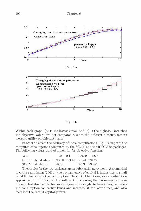
100 Chapter 6
Fig. 1a
Fig. 1b
Within each graph, (a) is the lowest curve, and (c) is the highest. Note thatthe objective values are not comparable, since the different discount factorsmeasure utility on different scales.
In order to assess the accuracy of these computations, Fig. 2 compares thecomputed consumptions computed by the SCOM and the RIOTS 95 packages.The following values were obtained for for objective functions:
κ = .0 0.1 0.8639 1.7278RIOTS 95 calculation 98.08 109.46 196.41 294.74SCOM calculation 98.08 195.96 293.85The results for the two packages are in substantial agreement. As remarked
in Craven and Islam (2001a), the optimal curve of capital is insensitive to smallrapid fluctuations in the consumption (the control function), so a step-functionapproximation to the control is sufficient. Increasing the parameter kappa inthe modified discount factor, so as to give more weight to later times, decreasesthe consumption for earlier times and increases it for later times, and alsoincreases the rate of capital growth.
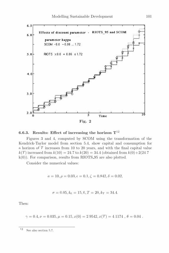
Modelling Sustainable Development 101
Fig. 2
6.6.3. Results: Effect of increasing the horizon T12
Figures 3 and 4, computed by SCOM using the transformation of theKendrick-Taylor model from section 5.4, show capital and consumption fora horizon of T increases from 10 to 20 years, and with the final capital valuek(T ) increased from k(10) = 24.7 to k(20) = 34.4 (obtained from k(0)+2(24.7−k(0)). For comparison, results from RIOTS 95 are also plotted.
Consider the numerical values:
a = 10, ρ = 0.03, ε = 0.1, ζ = 0.842, δ = 0.02,
σ = 0.05, k0 = 15, 0, T = 20, kT = 34.4.
Then:
γ = 0.4, ν = 0.035, µ = 0.15, x(0) = 2.9542, x(T ) = 4.1174 , θ = 0.04 .
12 See also section 5.7.
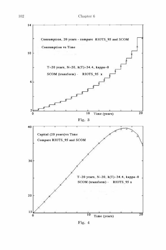
102 Chapter 6
Fig. 3
Fig. 4
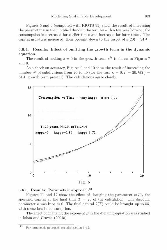
Modelling Sustainable Development 103
Figures 5 and 6 (computed with RIOTS 95) show the result of increasingthe parameter κ in the modified discount factor. As with a ten year horizon, theconsumption is decreased for earlier times and increased for later times. Thecapital growth is increased, then brought down to the target of k(20) = 34.4 .
6.6.4. Results: Effect of omitting the growth term in the dynamicequation.
The result of making δ = 0 in the growth term eδt is shown in Figures 7and 8.
As a check on accuracy, Figures 9 and 10 show the result of increasing thenumber N of subdivisions from 20 to 40 (for the case κ = 0, T = 20, k(T ) =34.4, growth term present). The calculations agree closely.
Fig. 5
6.6.5. Results: Parametric approach13
Figures 11 and 12 show the effect of changing the parameter k(T ), thespecified capital at the final time T = 20 of the calculation. The discountparameter κ was kept as 0. The final capital k(T ) could be brought up to 55,with some loss in consumption.
The effect of changing the exponent β in the dynamic equation was studiedin Islam and Craven (2001a).
13 For parametric approach, see also section 6.4.2.
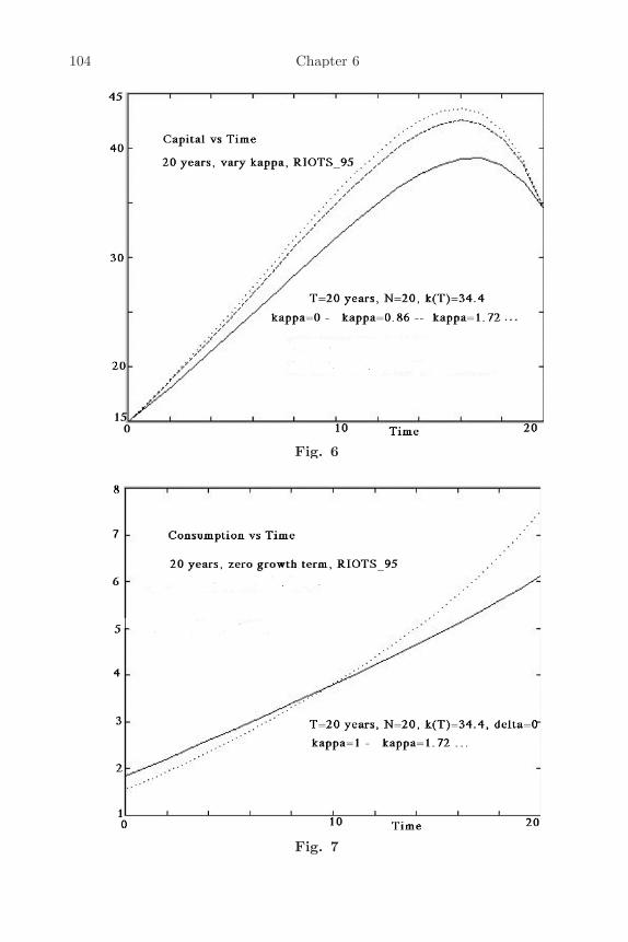
104 Chapter 6
Fig. 6
Fig. 7

Modelling Sustainable Development 105
Fig. 8
Fig. 9
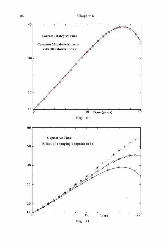
106 Chapter 6
Fig. 10
Fig. 11
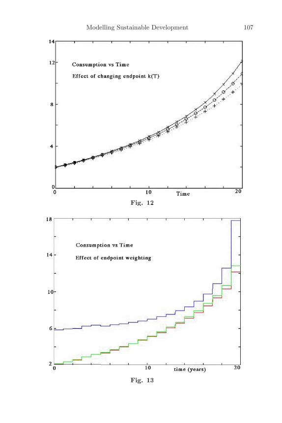
Modelling Sustainable Development 107
Fig. 12
Fig. 13
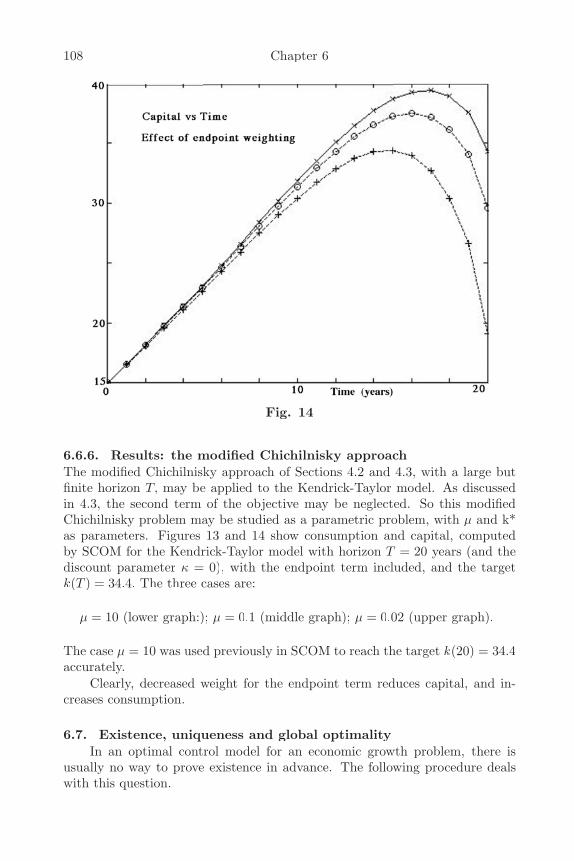
108 Chapter 6
Fig. 14
6.6.6. Results: the modified Chichilnisky approachThe modified Chichilnisky approach of Sections 4.2 and 4.3, with a large butfinite horizon T, may be applied to the Kendrick-Taylor model. As discussedin 4.3, the second term of the objective may be neglected. So this modifiedChichilnisky problem may be studied as a parametric problem, with µ and k*as parameters. Figures 13 and 14 show consumption and capital, computedby SCOM for the Kendrick-Taylor model with horizon T = 20 years (and thediscount parameter κ = 0), with the endpoint term included, and the targetk(T ) = 34.4. The three cases are:
µ = 10 (lower graph:); µ = 0.1 (middle graph); µ = 0.02 (upper graph).
The case µ = 10 was used previously in SCOM to reach the target k(20) = 34.4accurately.
Clearly, decreased weight for the endpoint term reduces capital, and in-creases consumption.
6.7. Existence, uniqueness and global optimalityIn an optimal control model for an economic growth problem, there is
usually no way to prove existence in advance. The following procedure dealswith this question.
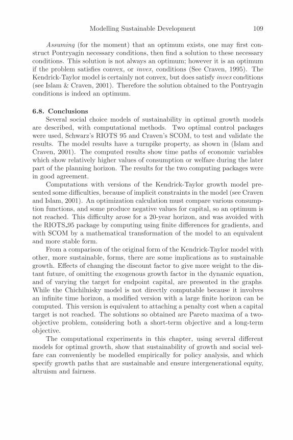
Modelling Sustainable Development 109
Assuming (for the moment) that an optimum exists, one may first con-struct Pontryagin necessary conditions, then find a solution to these necessaryconditions. This solution is not always an optimum; however it is an optimumif the problem satisfies convex, or invex, conditions (See Craven, 1995). TheKendrick-Taylor model is certainly not convex, but does satisfy invex conditions(see Islam & Craven, 2001). Therefore the solution obtained to the Pontryaginconditions is indeed an optimum.
6.8. ConclusionsSeveral social choice models of sustainability in optimal growth models
are described, with computational methods. Two optimal control packageswere used, Schwarz’s RIOTS 95 and Craven’s SCOM, to test and validate theresults. The model results have a turnpike property, as shown in (Islam andCraven, 2001). The computed results show time paths of economic variableswhich show relatively higher values of consumption or welfare during the laterpart of the planning horizon. The results for the two computing packages werein good agreement.
Computations with versions of the Kendrick-Taylor growth model pre-sented some difficulties, because of implicit constraints in the model (see Cravenand Islam, 2001). An optimization calculation must compare various consump-tion functions, and some produce negative values for capital, so an optimum isnot reached. This difficulty arose for a 20-year horizon, and was avoided withthe RIOTS 95 package by computing using finite differences for gradients, andwith SCOM by a mathematical transformation of the model to an equivalentand more stable form.
From a comparison of the original form of the Kendrick-Taylor model withother, more sustainable, forms, there are some implications as to sustainablegrowth. Effects of changing the discount factor to give more weight to the dis-tant future, of omitting the exogenous growth factor in the dynamic equation,and of varying the target for endpoint capital, are presented in the graphs.While the Chichilnisky model is not directly computable because it involvesan infinite time horizon, a modified version with a large finite horizon can becomputed. This version is equivalent to attaching a penalty cost when a capitaltarget is not reached. The solutions so obtained are Pareto maxima of a two-objective problem, considering both a short-term objective and a long-termobjective.
The computational experiments in this chapter, using several differentmodels for optimal growth, show that sustainability of growth and social wel-fare can conveniently be modelled empirically for policy analysis, and whichspecify growth paths that are sustainable and ensure intergenerational equity,altruism and fairness.
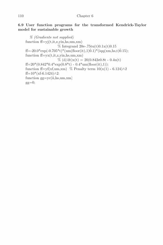
110 Chapter 6
6.9 User function programs for the transformed Kendrick-Taylormodel for sustainable growth
% (Gradients not supplied)function ff=yj(t,it,z,yin,hs,um,xm)
% Integrand 20e-.75tu(t)0.1x(t)0.15ff=-20.0*exp(-0.705*t)*(um(floor(it),1)0.1)*(iqq(xm,hs,t)0.15);function ff=yx(t,it,z,yin,hs,um,xm)
% (d/dt)x(t) = 20(0.842e0.8t - 0.4u(t)ff=20*(0.842*0.4*exp(0.8*t) - 0.4*um(floor(it),1));function ff=yf(xf,um,xm) % Penalty term 10(x(1) - 6.124)∧2ff=10*(xf-6.1424)∧2;function gg=yc(ii,hs,um,xm)gg=0;
Chapter 7Modelling and Computing a
Stochastic Growth Model7.1. Introduction
An economy progresses in an environment that is characterised by uncer-tain static and dynamic forces and processes. Uncertain factors which underliethe dynamic growth processes correspond to market prices, ecosystem, tech-nical progress, population growth, fluctuations in output, exports, imports,exchange rates, and economic and social factors. Social choice in an uncer-tain environment is more problematic and controversial than in a certain en-vironment (Islam, 2001). Models which incorporate these uncertain factorsin economic growth and development are useful for understanding uncertainprocesses of economic dynamics. A suitably specified stochastic model can beused to discuss social choice in uncertain conditions. This requires specifica-tion of a decision criterion, and an appropriate mathematical description of theuncertainty. This is feasible and plausible with the assumptions of new3 wel-fare economics. An earlier work on modeling stochastic growth is by Haavelmo(1954). Other contributions include Aoki (1989), Kendrick (1981), Tintner andSengupta (1969), and Sengupta and Fanchon (1997). Taylor and Uhlig (1990)provide an up to date exposition of methods for modeling non-linear stochasticoptimal growth economics, applied to a particular computational model. Otherreferences related to stochastic optimization in economics include Arrow (1951,1971), Islam (1999, 2001a), Kelly and Kolstad (1997), Radner (1982), Tapiero(1998).
Economic models including stochastic elements have been studied either(a) in continuous time, or (b) in discrete time. For continuous time, the stochas-tic elements are usually described by a Wiener process, for which the stochas-tic contributions from nonoverlapping time intervals are independent, howevershort the intervals. This may not happen in the real world. A discrete-timemodel, say with time intervals δ > 0, avoids this assumption, but may requireextensive calculations of probability distributions, e.g. for a Markov chain.However, if the stochastic elements are not too large, it may be enough tocompute the mean and variance, instead of the whole distributions.
A continuous-time deterministic model for economic growth and develop-ment may be approximated by a discrete-time model, by discretizing the time.If small stochastic terms are then added to this discrete-time model, dynamic(difference) equations may be obtained for the mean and variance. These lead,in turn, to continuous-time dynamic equations for mean and variance. Theyrelate to the original model, with small stochastic terms added, but now only
112 Chapter 7
assuming independence for contributions over non-overlapping time intervalsof length δ.
To explore this approach, a small stochastic term is added to the classi-cal (deterministic) Kendrick-Taylor model for economic growth (Kendrick andTaylor, 1971; Kendrick, 1981), considered as an optimal control model forcomputation (see Islam and Craven, 2000). Other classical growth models (seeChakravarty, 1969; Fox, Sengupta and Thorbecke, 1973) could be similarlymodified by adding a stochastic element. The computations were done usingthe RIOTS 95 package (see Schwartz, Polak and Chen, 1997), using MATLAB(see MATLAB, 1997). Other optimal control packages that might have beenused include SCOM (Islam and Craven, 2000), and MISER3 (Jennings, Fisher,Teo and Goh, 1991).
7.2. Modelling Stochastic GrowthConsider a dynamic model in continuous time, described by:
x(0) = x0, x(t) = m(x(t), u(t), t) + θ(t) (0 ≤ t ≤ T ),
with a stochastic term θ(t). Assume only that the stochastic contributions forsuccessive time intervals (jδ, (j + 1)δ), j = 1, 2, . . . are independent. Here x(·)is the state function, whose components may include capital, and terms de-scribing resource utilization and environmental factors, and u(·) is the controlfunction, which may describe consumption. Note that θ(·) is not assumed to bea Wiener process. Also, the stochastic terms can, in practice, be only knownapproximately; in particular, the distribution is never known precisely, and usu-ally only an approximate variance. So it may suffice to calculate the stochasticterm rather approximately, while the expectation (= mean) is calculated moreprecisely.
Now discretize the time, with time intervals δ, to obtain an approximatingdiscrete-time process for z(j) := x(δj and v(j) := v(δj as:
z(j + 1) − z(j) = m(z(j), v(j), δj) + ξ(j),
where the stochastic terms ξ(j) are now assumed independent. If the ξ(j) arenot too large, the mean and variance of z(j) can be sufficiently described bydifference equations. For convenient computation, the difference equations maybe approximated by differential equations in continuous time t. The result isa good approximation to the mean of x(t), and a useful approximation to thevariance of x(t), for the model described.
Other authors have considered approximating such models by discretizingin various ways the state space or the time. Taylor and Uhlig (1990) havesurveyed a number of such approaches for a discrete-time model of the form:
xt = ρxt−1 + εt,
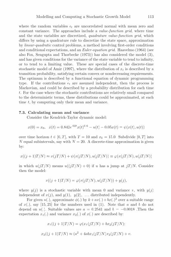
Modelling and Computing a Stochastic Growth Model 113
where the random variables εt are uncorrelated normal with mean zero andconstant variance. The approaches include a value-function grid, where timeand the state variables are discretized, quadrature value-function grid, whichdiffers by using a quadrature rule to discretize the state space, approximationby linear-quadratic control problems, a method involving first-order conditionsand conditional expectations, and an Euler-equation grid. Haavelmo (1964) (seealso Fox, Sengupta and Thorbecke (1973)) has also considered the model (3),and has given conditions for the variance of the state variable to tend to infinity,or to tend to a limiting value. These are special cases of the discrete-timestochastic model of Amir (1997), where the distribution of xt is described by atransition probability, satisfying certain convex or nondecreasing requirements.The optimum is described by a functional equation of dynamic programmingtype. If the contributions εt are assumed independent, then the process isMarkovian, and could be described by a probability distribution for each timet. For the case where the stochastic contributions are relatively small comparedto the deterministic terms, these distributions could be approximated, at eachtime t, by computing only their mean and variance.
7.3. Calculating mean and varianceConsider the Kendrick-Taylor dynamic model:
x(0) = x0, x(t) = 0.842e.02tx(t)0.6 − u(t) − 0.05x(t) ≡ ψ(x(t), u(t))
over time horizon t ∈ [0, T ], with T = 10 and x0 = 15.0 Subdivide [0, T ] intoN equal subintervals, say with N = 20. A discrete-time approximation is givenby:
x((j + 1)T/N) ≈ x(jT/N) + ψ(x(jT/N), u(jT/N)) ≡ ϕ(x(jT/N), u(jT/N))
in which u(jT/N) means u((jT/N) + 0) if u has a jump at jT/N. Considerthen the model:
x((j + 1)T/N) = ϕ(x(jT/N), u(jT/N)) + y(j),
where y(j) is a stochastic variable with mean 0 and variance v, with y(j)independent of x(j), and y(1), y(2), . . . distributed independently.
For given u(.), approximate φ(.) by k +ax(.)+ bx(.)2 over a suitable rangeof x(.), say [15, 25] for the numbers used in (1). Note that a and b do notdepend on u(.). Suitable values are a = 0.2541 and b = −0.0018 .Then theexpectation x1(.) and variance x2(.) of x(.) are described by:
x1((j + 1)T/N) = ϕ(x1(jT/N) + bx2(jT/N);
x2((j + 1)T/N) ≈ (a2 + 4abx1(jT/N)x2(jT/N) + v.
114 Chapter 7
The equation for expectation is approximate, but may be sufficiently accuratewhen the stochastic terms are small. It is based on the following calculation.If X and Y are stochastic variables, and Z = k + aX + bX2, then Z hasexpectation and variance given by :
EZ = k + aEX + b(EX)2 + bvarX;
varZ = varY + (a2 + 5b2(EX)2 + 4abEX))varX
+(4b2EX + 2ab)E(X3) + b2var(X2).
Then the equation for x2(t) is obtained by omitting some small terms, assumingb is not too large. Note that, as j increases, the variance x2(.) is increased bythe successive addition of terms v = varY , and also decreased because thepower 0.6, reflected in the negative coefficient b, reduces the contribution ofvarx(t)
These difference equations are now replaced by differential equations (incontinuous time):
x(t) = ψ(x1(t), u(t)) + (N/T )bx2(t);
x2(t) = (Nv/T ) + (N/T )(a2 − 1 + 4abx1(t))x2(t).
The rough approximation used here only affects the stochastic terms, whereasthe calculation of expectation is more precise. The objective function to bemaximized is:
J(u) =∫ 10
0
∫∫10.0(e−0.03t + κ)u(t)0.1 dt,
where κ is zero for the original Kendrick-Taylor model, and positive if greaterweight is given to the more distant future. The state function x(.) does notenter this objective function, so it is not necessary to consider its expectation.
This optimal stochastic growth model requires specification of a number ofparameters, including the rate of time discounting, the parameter κ describingthe weight to be given to the more distant future, the time horizon (taken hereas T = 10 years), the endpoint condition for the capital x(T ), and the varianceparameter v.
7.4. Computed results for stochastic growthThe computed results demonstrate the intertemporal optimal allocation
of resources in uncertain conditions (stochastic social choice). The followingdiagrams show the expected capital (Figure 1), the variance of the capital(Figure 2), and the consumption (Figure 3), as functions of time, with differentvalues of the parameter v, describing the variance of the stochastic term addedto the dynamic equation, and also when the endpoint constraint on the capitalat the end time T is changed. Here κ = 0.0, as in the original Kendrick-Taylor model. Figures 4,5,6 show comparable results when κ = 0.8639, a valueconsidered to describe greater weight given to times after the horizon T = 10.
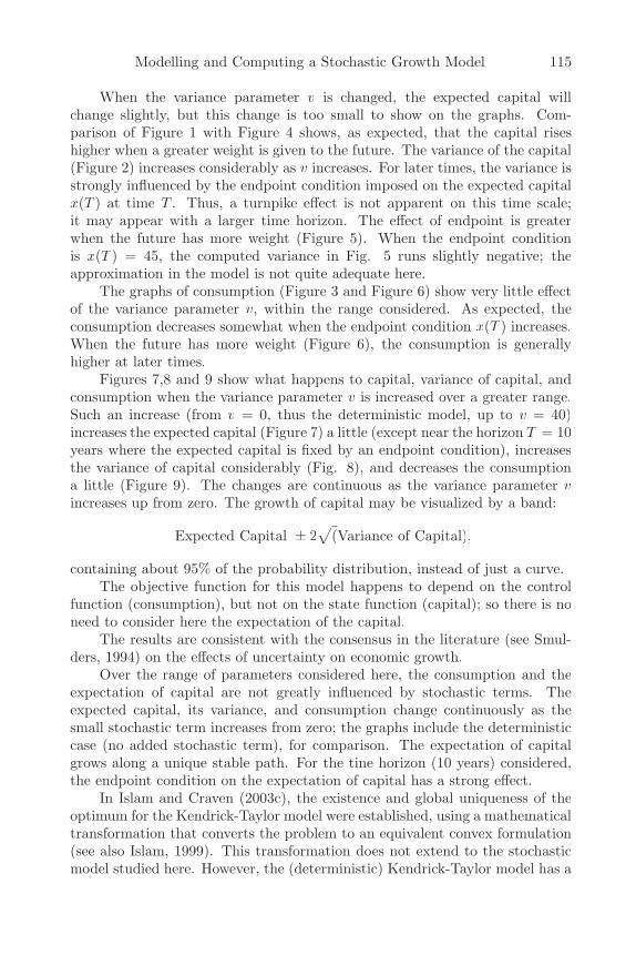
Modelling and Computing a Stochastic Growth Model 115
When the variance parameter v is changed, the expected capital willchange slightly, but this change is too small to show on the graphs. Com-parison of Figure 1 with Figure 4 shows, as expected, that the capital riseshigher when a greater weight is given to the future. The variance of the capital(Figure 2) increases considerably as v increases. For later times, the variance isstrongly influenced by the endpoint condition imposed on the expected capitalx(T ) at time T . Thus, a turnpike effect is not apparent on this time scale;it may appear with a larger time horizon. The effect of endpoint is greaterwhen the future has more weight (Figure 5). When the endpoint conditionis x(T ) = 45, the computed variance in Fig. 5 runs slightly negative; theapproximation in the model is not quite adequate here.
The graphs of consumption (Figure 3 and Figure 6) show very little effectof the variance parameter v, within the range considered. As expected, theconsumption decreases somewhat when the endpoint condition x(T ) increases.When the future has more weight (Figure 6), the consumption is generallyhigher at later times.
Figures 7,8 and 9 show what happens to capital, variance of capital, andconsumption when the variance parameter v is increased over a greater range.Such an increase (from v = 0, thus the deterministic model, up to v = 40)increases the expected capital (Figure 7) a little (except near the horizon T = 10years where the expected capital is fixed by an endpoint condition), increasesthe variance of capital considerably (Fig. 8), and decreases the consumptiona little (Figure 9). The changes are continuous as the variance parameter vincreases up from zero. The growth of capital may be visualized by a band:
Expected Capital ± 2√
(Variance of Capital),
containing about 95% of the probability distribution, instead of just a curve.The objective function for this model happens to depend on the control
function (consumption), but not on the state function (capital); so there is noneed to consider here the expectation of the capital.
The results are consistent with the consensus in the literature (see Smul-ders, 1994) on the effects of uncertainty on economic growth.
Over the range of parameters considered here, the consumption and theexpectation of capital are not greatly influenced by stochastic terms. Theexpected capital, its variance, and consumption change continuously as thesmall stochastic term increases from zero; the graphs include the deterministiccase (no added stochastic term), for comparison. The expectation of capitalgrows along a unique stable path. For the tine horizon (10 years) considered,the endpoint condition on the expectation of capital has a strong effect.
In Islam and Craven (2003c), the existence and global uniqueness of theoptimum for the Kendrick-Taylor model were established, using a mathematicaltransformation that converts the problem to an equivalent convex formulation(see also Islam, 1999). This transformation does not extend to the stochasticmodel studied here. However, the (deterministic) Kendrick-Taylor model has a
116 Chapter 7
strictly stable optimum, and the stochastic model considered is a small pertur-bation of the deterministic model. Hence, by Craven (1995), Theorem 4.7.1,an optimum exists for the stochastic model. However, this is not quite enoughto prove uniqueness, though this is likely.
Fig. 1
7.5. Requirements for RIOTS 95 M-filesCompared with the usual (deterministic) Kendrick-Taylor model, the num-
ber of states is increased from 1 to 2. The M-files sys h for the right hand sideof the dynamic equation, and sys dh for its gradient, take the following forms:
xdot = [0.842 ∗ exp(0.02 ∗ t) ∗ x(1) ∧ 0.6 − u(1) − 0.05 ∗ x(1) . . .
−2.0 ∗ 0.0028 ∗ x(2); . . .
2.0 − 2.0 ∗ (0.9354 + 0.00183 ∗ x(1)) ∗ x(2)];
(Here . . . is MATLAB’s code for “continued next line”. )
Modelling and Computing a Stochastic Growth Model 117
Fig. 2
Fig. 3
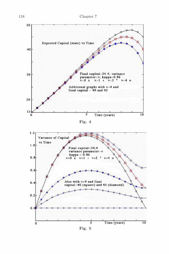
118 Chapter 7
Fig. 4
Fig. 5
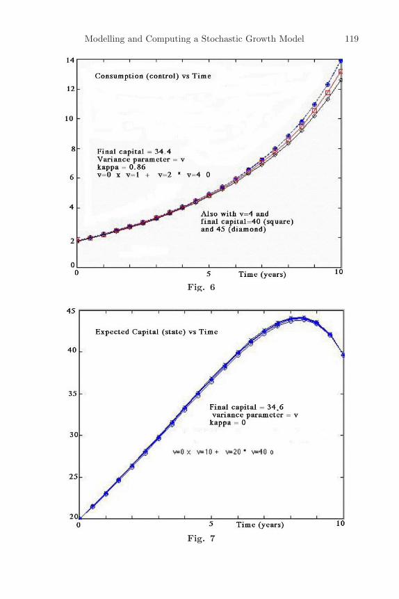
Modelling and Computing a Stochastic Growth Model 119
Fig. 6
Fig. 7
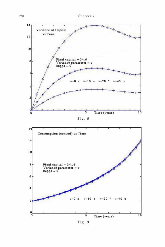
120 Chapter 7
Fig. 8
Fig. 9
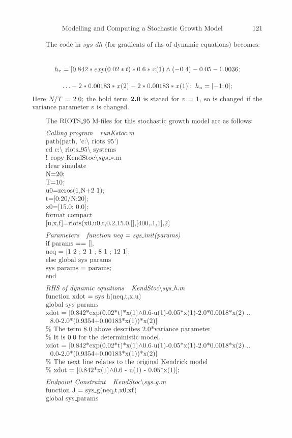
Modelling and Computing a Stochastic Growth Model 121
The code in sys dh (for gradients of rhs of dynamic equations) becomes:
hx = [0.842 ∗ exp(0.02 ∗ t) ∗ 0.6 ∗ x(1) ∧ (−0.4) − 0.05 − 0.0036;
. . . − 2 ∗ 0.00183 ∗ x(2) − 2 ∗ 0.00183 ∗ x(1)]; hu = [−1; 0];
Here N/T = 2.0; the bold term 2.0 is stated for v = 1, so is changed if thevariance parameter v is changed.
The RIOTS 95 M-files for this stochastic growth model are as follows:
Calling program runKstoc.mpath(path, ’c:\ riots 95’)cd c:\ riots 95\ systems! copy KendStoc\sys ∗.mclear simulateN=20;T=10;u0=zeros(1,N+2-1);t=[0:20/N:20];x0=[15.0; 0.0];format compact[u,x,f]=riots(x0,u0,t,0.2,15.0,[],[400,.1,1],2)
Parameters function neq = sys init(params)if params == [],neq = [1 2 ; 2 1 ; 8 1 ; 12 1];else global sys paramssys params = params;end
RHS of dynamic equations KendStoc\sys h.mfunction xdot = sys h(neq,t,x,u)global sys paramsxdot = [0.842*exp(0.02*t)*x(1)∧0.6-u(1)-0.05*x(1)-2.0*0.0018*x(2) ...
8.0-2.0*(0.9354+0.00183*x(1))*x(2)];% The term 8.0 above describes 2.0*variance parameter% It is 0.0 for the deterministic model.xdot = [0.842*exp(0.02*t)*x(1)∧0.6-u(1)-0.05*x(1)-2.0*0.0018*x(2) ...
0.0-2.0*(0.9354+0.00183*x(1))*x(2)];% The next line relates to the original Kendrick model% xdot = [0.842*x(1)∧0.6 - u(1) - 0.05*x(1)];
Endpoint Constraint KendStoc\sys g.mfunction J = sys g(neq,t,x0,xf)global sys params
122 Chapter 7
F NUM = neq(5);if F NUM == 1J = 0;elseif F NUM == 2J = xf(1) - 40.0;end
Integrand of Objective Function KendStoc\sys l.mfunction z = sys l(neq,t,x,u)global sys paramsF NUM = neq(5);if F NUM == 1z = -10.0*(exp(-0.03*t)+0.86394)*u(1)0.1;
% The parameter 0.86394 gives weight to future% The following line describes the original Kendrick model
% z = -10.0*(exp(-0.03*t)+0.0)*u(1)∧0.1;elsez = -x(1) + 0.3;end
Gradients for dynamic equation KendStoc\sys dh.mfunction [h x,h u] = sys Dh(neq,t,x,u)global sys paramsh x = [0.842*exp(0.02*t)*0.6*x(1)∧(-0.4)-0.05 -0.0036; ...
-2.0*0.00183*x(2) -2.0*0.00183*x(1)];h u = [-1 0];
Constraint Gradients KendStoc\sys dg.mfunction [J x0,J xf,J t] = sys Dg(neq,t,x0,xf)global sys paramsF NUM = neq(5);J x0 = [0 0 0]; J xf = [0 0 0];if F NUM == 1J x0(1) = 0;elseif F NUM == 2J xf(1) = 1;end
Gradients of Integrand KendStoc\sys dl.mfunction [l x,l u,l t] = sys Dl(neq,t,x,u)global sys paramsl x = 0;l u = -(exp(-0.03*t)+0.86394)*u(1)∧(-0.9);% The parameter 0.86394 gives weight to the future% The following line describes the original Kendrick model% l u = -(exp(-0.03*t)+0.0)*u(1)∧(-0.9);
Chapter 8
Optimization in Welfare Economics8.1. Static and dynamic optimization
Optimal social welfare is generally defined with Pareto’s mathematicaldefinition of optimality of a vector objective function (see section 2.8). Theanalysis of social welfare and social choice (see Arrow and Reynaud, 1986;Arrow, Sen and Susumura, 2003; Schulz, 1988) also depend on vector opti-mization. Economic developments of these ideas are presented e.g in Senguptaand Fox (1969), Ehrgott (2000). In Islam (2001a), such ideas are applioed todecentralized and to centrally planned economies. Social welfare cannot alwaysbe measured by summing individual utilities, and a vector of utilities must bestudied, with appropriate vector ordering (see e.g. Arrow and Scitovsski, 1969;Arrow and Intriligator, 1985; Sen, 1969). An economic model may maximize (inPareto’s sense) several competing welfare criteria or utilities ui(·), or maximizesome welfare function W (u1(·), u2(·), . . .), subject to constraints gi(x) ≥ 0, andperhaps also equality constraints. The classical economic assumptions of non-satiety of utility, and convexity of preference and production sets, are usuallymade here, but may be relaxed (see Schulz, 1988) for discussion of some non-classical models). The ui(·) could be utilities of individual agents. While thewelfare function is often taken as a weighted sum of individual utilities, theimplied assumption that one agent’s misfortune is compensated by another’sgood fortune is open to doubt. The usual assumption of convexity, underwhich a local optimun is a global optimum, is not always appropriate. Whenit fails, there may be multiple optima (see section 2.5). However, the methodsof section 2, and such concepts as invex, relaxing convex, still apply.
An economic model may be static, thus not time-dependent, or it may bedynamic, thus evolving in time. Dynamic models’ typically lead to optimal con-trol formulations. For the basic formulations, refer to sections 1.2, 2.1, 2.8 and2.13. Such models typically arise in optimal growth models, such as with al-location and social choice, sustainable resource management, intergenerationalequity, and economic planning. They contain conflicting economic objectives,such as consumption utility maximization, achieving full employment, inter-generational economic equity, sustainability, and environmental requirements.The models considered include economic growth, decentralized planning, col-lective utility, and resource depletion. A multiobjective optimum consists of aset of Pareto points, among which a choice must eventually be made by othercriteria (see Bolintineanu, 1993).
8.2. Some static welfare modelsA number of models have been given in Islam and Craven (2001b), and
are summarized here. The maximization of W (u1(·), u2(·), . . .), or the vector
124 Chapter 8
(Pareto) maximization of a vector objective {u1(·), u2(·), . . .),, may be restrictedby additional constraints, which put a floor below which no individual utilitymay fall. This adds extra terms to the Lagrangian condition (WKKT) foroptimality, so that the optimum is no longer a Pareto maximum for the originalmodel. The non-satiety property does not always apply. The utility for user imay be extended to:
u#i (x) := ui(x) +
∑j �=�� i
αijuj(x),
to give some weight, depending on the coefficients αij , to the welfare of otherusers. Denote the vector of these new utilities by MU(x), where U(x) :={u1(x), u2(x), . . . , un(x)), and M is a matrix made from the coefficients αij .The Pareto maximization of MU(x) is equivalent to the Pareto maximizationof U(x) with respect to a different order cone:
Q = M−1(Rn+);
see section 2.8.A welfare function W may give a good description only in some central
region, thus excluding outlying regions where some utility falls below a floor. Asecondary objective function, that need not be only a function of the objectivecomponents, may be used to optimize over the set of Pareto optimum points(see Bolinteanu, 1993a, b), and this will determine a set of weights for theobjective components. This may bear on the question of impossibility (Arrow,1951; Arrow and Reynaud, 1996) or possibility (Sen, 1970).
In a cooperative game model described by Cesar (1994), agent i has hisown objective function J i(.), and a weighted payoff function
∑wiJ
i (x) is tobe maximized, subject to the state vector x in a suitable feasible region X. Thisgives one of the Pareto maxima of the vector function:
J(.) := (J1(, ), J2(.), . . .)
over X, depending on the choice of weights wi.However, there are other game models to which invexity and related ideas
may be applied. A zero-sum competitive game for two players leads to a mini-max model, where there is a single objective function J(u1, u2 ), which player1 maximizes with respect to u1 , and player 2 minimizes with respect to u2 ,subject to constraints g(u1 ) ≤ 0 and k(u2 ) ≤ 0. Define a Lagrangian functionas:
L(u1, u2; v1, v2) := J(u1, u2) : −v1g(u1) + v2k(u2).
Under some (non-trivial) regularity assumptions (Craven, 1988), it is necessaryfor a minimax that the gradient of this Lagrangian with respect to (u1, u2)is zero, for some non-negative multipliers v1, v2 , together with v1g(x1) =
Optimization in Welfare Economics 125
0, v2k(x2) = 0. These conditions are sufficient for a minimax under appropriateinvexity assumptions (Craven, 1988).
A welfare model, described in Leonard and Long (1992) and Schulz (1988)has I individuals, G goods, R resources, and amount YrYY available of resourcer. In terms of the state variables xi
g = amount of good g used by individual iand yrg = amount of resource r used to make good g, a welfare function:
W (U1(x11, . . . , x
1G), . . . , U I(xI
1, . . . , xIG )) ≡ W (U1(x1), . . . , U I(xI)),
is maximized, subject to nonnegative variables and constraints:
aixig = FgFF (y1g, . . . , yRg ) ≡ FgFF (yg) (g = 1, 2, . . . , G)
∑g
cgyrg = br (i = 1, 2, . . . , R).
The Lagrangian is:
L(.) = W (U1(x1), . . . , U I(xI)) +∑
g
πg[FgFF (byg)−∑
i
aixig]
+∑
r
λr[br −∑
g
cgyrg]
So necessary KKT conditions for a maximum are:
(∂W/∂U i)(∂U i/∂xgi) − πgai = 0(i = 1, 2, . . . , I).
If these conditions are sufficient, which happens if −W (U1(·), . . . , U I(·)) andthe constraint functions are invex with the same scale factor, then equilibriumconditions follow, thus under weaker assumptions than the usual ]convex W andlinear constraints. Otherwise, a quasimax of the welfare function is obtained,or a vector quasimax of the vector optimization problem.
A multiobjective optimum consists of a set of Pareto points, among which achoice must eentually be made by other criteria (see Bolintineanu, 1993). In themodels discussed here, some changes in the model, such as adding “unselfish”utility terms, result in moving from one Pareto point of the original model toanother. While each set of positive weights for the objectives determines oneor more Pareto points, and each Pareto point determines one or more sets ofweights, the weights are not an a priori choice by a decision maker, but maychange during computation (see section 8.5). Moreover, a point satisfying theKarush-Kuhn-Tucker (KKT) conditions (or equivalent Pontryagin conditionsfor optimal control) is not necessarily a maximum.
8.3. Perturbations and stabilityThe extended welfare model of section 8.2 with utilities u#
i (x) may beconsidered as Pareto maximizing the original utilities ui(x) with respect to a
126 Chapter 8
different (larger) order cone, and so the optima occur with some different valuesof the weights for the objectives, specified by the multiplier τ in WKKT.
A Pareto optimum p is locally proper (Craven, 1990) if the ratios of differ-ence of objectives, (uj(x) − ui(x)), are bounded when x is in some neighbour-hood of p. (For comparison, Geoffrion’s proper Pareto maximum (Geoffrion1968) considers all x.) Then (Craven, 1990) a Pareto maximum p is locallyproper exactly when the multiplier τ > 0, thus when each component τiττ > 0.This dsescribes a sort of stability of the objective components near a properPareto maximum; there is a bound to how fast they change. There is anequivalent stability property also for weak quasisaddlepoint (see section 2.9),described in Craven (1990).
Consider now a linearization of the welfare model with utilities ui(x)around a Pareto maximum p, and approximate the extended welfare model.with αij replaced by εαij , by a perturbation of this linearized model, with asmall parameter ε. The model is then a multi-objective linear program MLP,including a parameter ε. For a chosen set of weights for the objective compo-nents, specified by τ , there results a linear program, with a small perturbationapplied to the objective, but not to the constraints. A standard theory applieshere. The point p is generally a vertex of the (polyhedral) fceasible region(satisfying the constraints), and p is not moved by the perturbation if ε is suf-ficiently small. Thus a standard welfare model will give some (small) weight tothe welfare of other users.
8.4. Some multiobjective optimal control modelsCraven and Islam (2003) give a multiobjective version of the decentralized
resource allocation model of Arrow and Hurwicz (1960) (also Sengupta and Fox,1969, page 62). If there are n producers, and now n objective functions, thena Pareto maximum of the vector function
{f1(x1), f2ff (x2), . . . , fnff (xn)}may be considered, instead of a maximum of the sum of these components. Theeffect is to maximize
∑τiττ fiff (x) subject to constraints xi ∈ Xi,
∑gi(xi) ≤ b,
with non-negative weights τiττ which sum to one. Different Pareto maxima arisefrom different choice of τ . If τ is fixed, and a convex problem is assumed, thenthere is a dual problem:
MINv
∑i
(mi(v) + vb/n),
where v is a price attached to resource usage, and
mi(v) = MAX(τiττ fiff (xi) − vgi(x) subject to (∀i) xi ∈ Xi.
However, the convex assumption may be reduced to invex; thus, if xi ∈ Xi ⇔ξi(x) ≤ 0, and if all the functions −fiff , ξi, g are invex with the same scalefunction.
Optimization in Welfare Economics 127
Craven and Islam (2003) also presented an economic growth model involv-ing two conmumption (control) variables, and one capital (state) variable k(t).This model is now extended to r consumption variables cj(t). Motivated by theKendrick-Taylor model (see section 4.2), consider the dynamic equation:
k(0) = k0, k(t) = b(t)ξ(k(t)) −∑
ci(t) (0 ≤ t ≤ T ),
and a vector objective to be maximized, with components:
F iiFF (k, c) =
∫ T
0
∫∫e−ρtU i(k(t), c(t), t)dt − Qi(k(T )),
with c(t) := (c1(t), . . . , cr(t)) and utilities
U i(k(t), c(t)) = ci(t)σ + α∑q �=�� i
cq(t)σ,
in which (as in section 2) each user allows some weight to the welfare of otherusers. For this model, the Hamiltonian is:
∑τiττ {e−ρtU i(k(t), c(t), t)} − λ(t)(ξ(k(t)) −
∑ci(t)).
So the adjoint differential equation for the costate λ(t) is:
−λ(t) = λ(t)ξ′(k(t)), λ(T ) = µ(k(T ) − k∗),
with a weight µ and a constant k∗ chosen so that a given terminal constrainton k(T ) is satisfied (see section 2.1). If the controls ci(t) are not subject toany active constraints, then Pontgryagin’s principle requires that the gradientof the Hamiltonian with respect to the controls is zero. This gives:
e−ρtτ∗iττ σ(ci(t))σ−1 + λ(t) = 0,
where τ∗iττ := τiττ +
∑q �=�� i ατqττ is a modified multiplier for FiFF . So here again the
result of giving weight to the welfare of other users is to modify the multipliersattached to the objective components.
The behaviour is similar for a collective utility or welfare moldel, wherethe objectives to be maximized are:
∫ T
0
∫∫e−rhot
∑q
MiqMM U((cq(t))),
where U(·) is a utility function, ci(t) is consumption for user i,, k(t) is capi-tal stock, and thne matrix M of non-negative components MiqMM describes theweighting each user gives to the others. This model may describe an altruistic
128 Chapter 8
social welfare planning model. As before, if there are no active constraints onthe controls, then the multiplier vector τ when M is the identity matrix isshifted to MT τ .
8.5. Computation of multiobjective optimaIf weights τiττ are chosen for the objectives multiobjective problem, then a
scalar objectine∑
τiττ FiFF (·) may be optimized, by the methods usual for the con-strained optimization of a single objective. For dynamic problems, differentialequations must then be solved (see chapter 3.) But since the correct weightsare seldom known a priori, it is usual to supply a decision maker (DM) withtradeoff information on the effects of changing the balance between the sev-eral objectives, so that the DM may prescribe a direction in which to changethe weights. Often goal programming is used, this minimizing a weighted sumof deviations from goals, or targets (see e.g. Rustem, 1998). However, thisweighting depends implicitly on the chosen scales of measurement for the sev-eral objectives.
Since Pareto optimal points are many, every opportunity should be takento reduce the region to be searched. This may be done by placing bounds (e.g.floors) on some quantities, or on ratios of some objectives, where appropriate.
A secondary objective function may be optimized over the Pareto set (seeBolintineanu and Craven, 1992). This process is, to some extent, modelling thedecision maker.
The choice of parameters, which may be varied in a secondary optimiza-tion, whether by a decision maker or by a computer model, may be critical tothe understanding of a complicated multi-dimensional situation. If there areseveral objectives to be optimized, say F1FF (x), F2FF (x), F3FF (x) over some regionE, then it may be appropriate to choose one objective, say F1FF (x), as of firstimportance, and then to maximize the single objective F1FF (x) over E, subject toadditional inequality constraints, such as F2FF (x) ≥ p1, F3FF (x) ≥ p2, on the otherobjectives. There remains a secondary optimization over suitable values of theparameters p1 and p2. However, these are likely to have a more direct meaning,say in a busines situation, than would the tradeoffs between objectives.
All these details are relevant, both for computing a static problem, andfor computing a dynamic problem. For a static problem, any of the standardcodes for constrained nonlinear optimization (or for linear programming, if theproblem is linear) may be used. For a dynamic problem, the evaluation offunction values and gradients requires the solution of differential equations (fora problem in continuous time), or of difference equations (for a problem indiscrete time). The computational aspects for a problem in continuous timeare described in chapter 3.
Furthermore, for a dynamic (optimal control) model, there are severaladditional kinds of parametric constraints that may be appropriate. If somequantity v(t) is to be constrained, then the possibilities include:
• a pointwise bound: (∀t) v(t) ≥ p;
Optimization in Welfare Economics 129
• an average bound:∫ T
0
∫∫w(t)v(t)dt ≥ p with some weighting function
w(t);• in the case of stochastic optimal control (see chapter 7, and the portfoliomodels described in Sengupta and Fanchon, 1997; Tapiero, 1996, Ziembaand Vickson, 1975, for examples), some probabilistic bound may beappropriate, such as
Prob{(∀t)v(t) ≥ p} ≥ 0.9;
With some of these bounds (when behaviour at several times is combined),the Pontryagin principle does not apply; however KKT conditions are stillapplicable.
8.6. Some conditions for invexityAn optimal control problem has an equality constraint, the dynamic equa-
tion. Consider the problem (with a single objective F ):
MIN F (z) subject to G(z) ≤ 0,K(z) = 0.
Let p be a KKT point, with multipliers λ and µ. Assume the following version(Type I) of invexity (Hanson and Mond, 1987):II
(∀z)F (z) − F (p) ≥ F ′(pη(z, p); −G(p) ≥ G′(p)η(z, p); 0 = K ′(p)η(z, p).
If z satisfies the constraints, then:
F (z)−F (p) ≥ F ′(p)η(z, p) = −λG′(p)η(z, p)−µK ′(p)η(z, p) ≥ λG(p)+ 0 = 0,
so a minimum is reached. If instead F is vector valued, then F is replaced byτF , and τ(F (z) − F (p)) ≥ 0 follows, proving that p is a weak minimum.
In an optimal control problem, z is replaced by the state and control (x, u),and p by a point (x, u) satisfying the Pontryagin conditions. If the problem iswritten (see section 2.2) as:
MINF (x, u), subject to Dx = M(x, u), G(x, u) ≡ G(u) ≤ 0,
then the required invexity takes the form:
F (x, u) − F (x, u) ≥ FxFF α + Guβ, G(u) ≥ Guβ, 0 = (D+MxMM )α + MuMM β,
in which the two components α(x, u; x, u) and β(x, u; x, u) replace η(z, p), andFxFF , etc. denote partial derivatives at (x, u).
A composite function f(g(.)), where g : Rn → Rm+ and f : Rm
+ → R aredifferentiable, is invex at p if g is invex, f is convex at q (where q = g(p))

130 Chapter 8
and f ′(q) has positive components, since (Craven and Islam, 2003), settingF (z) := f(q + z) − f(q), g(x) − g(p) ≥ g′(p)η(x, p), hence:
f(g(x)) − f(z(p)) = F (q + g(x) − g(p)) = F (q + g(x) − g(p)) − F (0)
≥ F ′(0)(g(x) − g(p)) = f ′(q)(g(x) − g(p) ≥ f ′(q)g′(p)η(x, p).
It is sometimes possible to replace an equality constraint by an inequal-ity constraint. One example is an economic growth model, with a terminalconstraint k(T ) = kT on the capital k(t). If the model maximizes some utilitydepending on consumption, then the terminal constraint may often be replacedby an inequality k(T ) ≥ kT , since the maximization tends to reduce k(T ). Insuch a case, the sign of the Lagrange multiplier for this terminal constraint isalready determined by the inequality.
8.7. DiscussionWhile welfare economic models are usually based on convex assumptions,
some relaxation to generalized convexity is possible (see e.g. Schaible andZiemba, 1981.) The less restrictive invex assumption allows various non-classical economic situations to be modelled. The quasimax concept provides adescription of a stationary point, without specifying the Lagrange multipliersfor the constraints. The discussion of shadow prices is related to a quasidualproblem also not requiring convex assumptions.
The weights for objective components, in a vector optimization model, arenot assigned a priori, but arise in the theory as multipliers. They are relatedto the stability of the model to perturbations, and they may change during acomputation.
Chapter 9Transversality Conditions for
Infinite Horizon9.1. Introduction
Economic and finance models for dynamic optimisation, expressed as op-timal control over an infinite time horizon, have been much discussed byeconomists, since many issues in social choices have everlasting implications.However, there has been controversy about the form and validity of terminalcostate conditions (transversality conditions) as time tends to infinity. In thischapter, such terminal conditions are proved: (i) when state and control tendto finite limits, and some likely assumptions about signs of gradients hold, (ii)when state and control tend to limits, with a restriction on the rate of conver-gence, and (iii) for growth models, when normalization by dividing by a growthfactor leads to a model of type (ii). These cases cover many of the economicand finance models of interest. Some of these have definite social choice ap-plications in the context of new3 welfare economics. The analysis leads to adiscussion of shadow prices, conditions sufficient for an optimum, and possiblecomputational approaches for infinite-horizon models.
9.2. Critical literature survey and extensionsEconomic models, especially for optimal growth and development, or for
behaviour in time of a financial process, often lead to optimal control problems,over a finite time interval [0, T], or an infinite time interval [0,∞). Typically,the model is described by a state function x(t) (usually vector-valued), de-scribing e.g. capital accumulation, and a control function u(t), describing .e.g.consumption. An objective, expressed as an integral involving the state andcontrol, is optimized, subject to a dynamic differential equation, and constraintson the control. Under some standard assumptions, conditions necessary for amaximum or minimum of such a model over [0, T] consist of the following:
(i) the dynamic differential equation for a state function x(t), with aninitial condition for x(0), and perhaps a terminal condition for x(T );(ii) an adjoint differential equation for a costate function λ(t), with aterminal condition on λ(T ); and(iii) Pontryagin’s maximum (or minimum) principle, that a Hamiltonianfunction is optimized, with respect to the control function u(t), at theoptimal control.Note that the standard assumptions include the restriction that any con-
straints on the control function apply to each time separately, thus excludingany restriction on the rate of change of the control, or any compensation be-
132 Chapter 9
tween controls at different times. If (as with some economic models) the controlis not constrained, then (iii) may be replaced by a weaker requirement, thatthe gradient of the Hamiltonian with respect to control is zero, and the as-sumptions are less stringent. The costate function, in an economic model, hasthe significance of a shadow price or a shadow cost.
The necessary conditions (i), (ii) and (iii) are not generally enough to implyan optimum. They become also sufficient conditions for a global optimum ifthe functions defining the control problem possess suitable convex properties,or (less restrictively) invex properties. This does not work if the terminalcondition on λ(T ) is omitted, since the system then is not completely defined,except in the special case when the terminal state x(T ) is completely specified(with T fixed), for then λ(T ) is free. This terminal condition on λ(T ) has oftenbeen called a transversality condition, for historical reasons deriving from time-optimal problems, where the (variable) time T to reach a target is minimized. Inthat situation, the transversality condition appears as a description of how theoptimal path crosses a terminal line (graphing state against T, as in Chiang(1992). Sethi and Thompson (2000) have presented λ(T ), for various caseswhen T is finite. (Some more general cases are also possible; see section 9.4.)
Transversality conditions have been much discussed (e.g. Leonard andLong, 1992; Burmeister and Dobell, 1970; Sengupta and Fanchon, 1997) foreconomic and financial models. Agenor and Montiel (1996) cited a modified´transversality condition for infinite horizon (see section 4). Cuthbertson (1996)has reported another sort of transversality condition for a financial model withconstant expected returns. However, a transversality condition is not signifi-cant on its own, but only as part of a complete set of necessary (and perhapsalso sufficient) conditions. Judd (1998) discusses some economic models wherethe Euler equation (equivalent to the adjoint differential equation) without itsterminal condition allows solutions which contradict economic requirements,so that a terminal condition is needed. (But it is already part of the neces-sary conditions). Moreover, the form of a transversality condition depends onfeatures of the model, namely the terminal condition (if present) on the statefunction, and the endpoint term (if present) in the objective function. It ispertinent to consider how these two features affect such questions as stabilityof the model. Islam and Craven (2003b) have considered dynamic optimizationmodels in finance, including cases of multiple steady states.
The role of the transversality conditions in economic and finance modelshas been summarized by Sengupta and Fanchon (1997, page 240), as:
“These conditions, often stated in terms of the adjoint (also called costate)variables, or the Lagrange multipliers associated with the dynamic equations ofmotion, seek to guarantee three things: uniqueness of the optimal trajectory,stability in the sense of convergence of the optimal path, and a condition ofperfect foresight of the future.”
It is remarked that uniqueness does not always occur for a non-convexmodel (Blanchard and Fischer, 1989), and that in the case of an infinite horizon
Transversality Conditions for Infinite Horizon 133
T (see section 3), some assumption about convergence of the optimal path isrequired to derive the transversality conditions. For such growth and financemodels for an infinite horizon without a discount factor, the objective functionis generally infinite. Following Ramsey (1928), this difficulty is avoided byconsidering a modified objective
∫ ∞0
∫∫[f(x(t), u(t))−B}dt, where the bliss point
B is a limiting value as time t → ∞. But this modified objective will also divergeto an infinite value, unless the state and control are supposed to convergesufficiently fast (e.g. as e−βt) to limiting values. Thus some assumption onconvergence rates is already implicit in standard economic models. However,any analysis of uniqueness and stability for a dynamic model in economics andfinance must include the correct transversality conditions.
Blitzer, Clarke and Taylor (1975) consider a model for finite horizon, whoseobjective is a utility function of consumption, plus an endpoint term depend-ing on final capital. Several terminal conditions (at the finite horizon) arediscussed, including a linear relation between final capital and consumptionrate, and a lower bound for the final capital (thus attaching a value to capitalafter the horizon time). Versions of such conditions might also be applied toinfinite-horizon problems.
Models with an infinite time domain [0,∞) are of economic significance.The standard Pontryagin theory does not immediately apply to an infinitetime domain. Some authors (e.g. Leonard and Long, 1992) have applied thestandard theory to a problem truncated to [0, T], with a terminal conditionthat λ(T ) equals the value of the costate at T for the infinite-domain problem.This obtains (ii) and (iii) for finite times t, but not a terminal condition onλ(t) as t tends to infinity. Some authors have postulated such a condition(without adequate proof), since it is required to obtain sufficient conditions foran optimum.
Michel (1982) analysed an infinite-horizon model, with no terminal con-straint on the state (trajectory), and obtained the transversality conditionλ(t) → 0 as t → ∞ under some restrictions (non-negative objective integrand,optimal state contained in a suitable neighbourhood of feasible solutions). How-ever, these (and other) assumptions “depend on properties of the optimal tra-jectory to be determined”. Janin (1979) showed that λ(t) → 0 at an exponentialrate (|λ(t)| ≤ const e−αt ) for a class of growth models with infinite horizon, noterminal constraint on the state, a restriction (a coercivity constraint) on thedynamic equation, and a discount rate not too small. Although transversalitydoes not always hold, the counter-examples of Halkin (1974) and Shell (1969)are (see Chiang, 1992) of an untypical character (the objective depends only onthe terminal state and control). However, the derivation of transversality con-ditions for infinite horizon, including more general cases such as λ(t)x(t) → 0,requires more analysis than “let T tend to infinity” in various authors. Michel(citing Janin, 1979) mentions requirements of “fast convergence”; sometimesthese are implied by the assumption that an optimum is reached with a finiteobjective. In some financial models (see Cuthbertson, 1996), where an assump-

134 Chapter 9
tion that “expected returns are constant” replaces an optimization, a terminalcondition is obtained, that a function of dividends tends to zero as time tendsto infinity; this is also called “transversality”.
Some economists have considered the case when the state and the controleach tend to limits as t tends to infinity (see e.g. the discussion in Judd,1998). But this does not generally happen for infinite-horizon models, especiallyif there are growth factors. The values of these limits need not be initiallyspecified; an optimization calculation will find them. In this case, one mayconsider (see section 4) a nonlinear transformation of time t in [0,∞) to scaledtime τ in [0,1], constructing τ by a suitable increasing function of t. Becauseof the assumed limits, τ = 1 is in the domain of the problem (whereas t = ∞is not). However, the transformed functions corresponding to m and f maybecome unboundedly large, as t tends to 1, upsetting the calculation. Thissituation is avoided if x(t) and u(t) converge sufficiently fast to their respectivelimits, as t tends to infinity. This leads to the expected (if not always proved)terminal conditions.
This chapter extends the literature in this area, by presenting three ap-proaches to terminal (transversality) conditions for the costate function, forinfinite horizon. These are listed as follows:
(a) There is a substantial class of infinite-horizon models, discussed insection 4, with the final state unrestricted, for which the terminal conditionλ(t) → 0 as t → ∞ is a consequence of some assumptions about signs ofgradients, and the assumed attainment (existence) of a finite optimum for theinfinite horizon. However, the condition λ(t)x(t) → 0 does not necessarilyfollow. An example is given where the state is unbounded, tending to no limit,and λ(t) → 0 is not enough to determine a unique costate λ(.). Applyingthe method of section 9.4 to problems where control and state tend to finite(unconstrained) limits, gives a large class of models where it is proved that thecostate tends to zero, and this is the correct transversality condition to showsufficiency, under e.g. convexity or uniqueness assumptions.
(b) When terminal conditions on the state are imposed, involving theassumption that state and control tend to some limits as t → ∞, then terminalconditions for λ(t) as t → ∞ are obtained in section 9.5, assuming that theconvergence to these limits is not too slow (it must be fast enough that certainintegrals have finite values).
(c) For some growth models, where limits are not reached, the state andcontrol may be normalized (see section 9.6) by dividing by some growth factor(e.g. an exponential growth, or a power of t), so that case (b) applies to thenormalized state and control. This approach solves the example cited in (a).
The economic interpretation of the costate λ(t), and other multiplierswhich occur, in terms of shadow prices is discussed in section 9.7. Sufficientconditions for a (global) optimum, involving generalized convex (invex) as-sumptions, relaxing the usual convex assumptions, are discussed in section 9.8.Dynamic modelling under non-convex assumptions has been studied (see e.g.

Transversality Conditions for Infinite Horizon 135
Islam and Craven, 2004 ), but some questions remain to be answered.The nonlinear time transformation has computational consequences (see
section 9.9). If x(t) and u(t) tend to limits, then the functions in the problem(the right side of the dynamic equation, and the integrand of the objective func-tion to be optimized) are changing only slowly when t is large. A descriptionusing scaled time τ can have the rates of change more uniform over τ in [0,1],than is possible over t in [0,∞). Consequently, a computation using scaled timemay be practicable, perhaps only needing a moderate number of subintervalsfor the discretization, when a direct computation using original time t may beimpracticable (see Craven, de Haas and Wettenhall, 1998).
Section 9.10 gives some discussion of special aspects of financial models.
9.3. Standard optimal control model for economic growth and finan-cial dynamics14
Consider the following model, with a state function x(t) (e.g. capital stock)and a control function u(t) (e.g. consumption):
MAX∫ T
0
∫∫e−δtf(x(t), u(t))dt + Φ(x(T ))
subject to:x(0) = x0, x(t) = m(x(t), u(t), t), q(x(T ) = 0,
a(t) ≤ u(t) ≤ b(t) (0 ≤ t ≤ T).
Here T is finite and fixed; the endpoint constraint q(x(T )) = 0 is not alwayspresent; constraints on the control u(t) are not always explicitly stated, al-though an implicit constraint u(t) ≥ 0 is commonly assumed. If q(.) or Φ(.)are absent from the model, they are replaced by zero.
Necessary Pontryagin conditions for a minimum of this model have beenderived in many ways. In Craven (1995), the control problem is reformulatedin mathematical programming form, in terms of a Lagrangian:
∫ T
0
∫∫[e−δtf(x(t), u(t)) + λ(t)m(x(t), u(t), t) − λ(t)x(t) − α(t)(a(t) − u(t))
−β(t)(u(t) − b(t) − 12µ[Φ(x(t) − µ−1ρ]2+ − 1
2µ[q(x(T ) − µ−1ν]δ(t − T )] dt.
with the costate λ(t), and also α(t) and β(t), representing Lagrange multipliers,µ a weighting constant, ρ and ν are Lagrange multipliers, and δ(t−T ) is a Diracdelta-function. Here, the terminal constraint on the state, and the endpointterm Φ(x(T )) in the objective, have been replaced by penalty cost terms in the
14 See also sections 2.2, 6.3.3, and 6.5.2.
136 Chapter 9
integrand; the multipliers ρ and ν have meanings as shadow costs. (This hasalso computational significance − see section 8. The solution of a two-pointboundary value problem, when x(T ) is constrained, has been replaced by aminimization.)
Then necessary Karush-Kuhn-Tucker (KKT) conditions follow. The ad-joint differential equation (ii) follows from one part of KKT (the Lagrangianfunction has zero gradient with respect to x), integrating the term λ(t)x(t)by parts; an integrated term λ(T )x(T ) arises, leading to a terminal conditionλ(T ) = 0 in case x(T ) is free (thus, unconstrained). Other contributions toλ(T ) come from q(.) and Φ(.), integrating the delta-function. The Pontryaginprinciple (iii) follows eventually, under some assumptions (such as boundedsecond derivatives of the functions f and g) from the other part of KKT (zerogradient of the Lagrangian with respect to x). Note that the proof requiresa finite horizon T, and that the control constraints apply to each time t sep-arately. The requirement of bounded second derivatives can be weakened torequire that they are majorised by some function with finite integral.
The adjoint differential equation is obtained in the form:
−λ(t) = e−δtfxff (x(t), u(t)) + λ(t)mx(x(t), u(t), t),
where fxff and mx denote partial derivatives with respect to x(t), together witha boundary condition (see Craven, 1995):
λ(T ) = Φx(x(T )) + κqx(x(T )),
in which Φx and qx denote derivatives with respect to x(T ), and κ is a Lagrangemultiplier, representing a shadow cost attached to the constraint q(x(T )) = 0.The value of κ is determined by the constraint that q(x(T ) = 0. If x(T ) is free,thus with no terminal condition, and Φ is absent, then the boundary conditionis λ(T ) = 0 . Note that x(T ) may be partly specified, e.g. by a linear constraintσT x(T ) = b (or ≥ b), describing perhaps an aggregated requirement for severalkinds of capital. In that case, the terminal constraint differs from λ(T ) = 0.
A diversity of terminal conditions for λ(T ) have been given in the eco-nomics literature (e.g. Sethi and Thompson, 2000); they are particular cases ofthe formula given above. For the constraint q(x(T )) ≥ 0, the multiplier κ ≥ 0.
9.4. Gradient conditions for transversalityThere is a class of optimal control problems over infinite time, including
some economic growth and dynamic finance models, where the boundary con-dition λ(t) → 0 for costate follows without special assumption, supposing thatan optimum is reached. Assume that the optimal control problem:
MAX∫ ∞
0
∫∫f(x(t), u(t), t)dt subject to
x(0) = 0, x(t) = m(x(t), u(t), t), g(u(t)) ≥ 0 (0 ≤ t < ∞),
Transversality Conditions for Infinite Horizon 137
where f (.,.,.), m(., ., .) and g(.) are differentiable functions, reaches an optimumat the point (x(.), u(.)) = (x∗(.), u∗(.)). (Usually this requires a discount factore−δt included in f.) Then the truncated problem, for finite T:
x(0) = 0, x(t) m(x(t), u(t), t), g(u(t)) ≥ 0 (0 ≤ t < ∞),
reaches an optimum when (x(t), u(t)) = (x∗(t), u∗(t)) for t < T. Assuming thatu∗(.) > 0, and that a constraint qualification, necessary Lagrangian conditionshold, in terms of a costate function λ(.):
−λ(t) = fxff (x∗(t), u∗(t), t) + ψ(t)mx(x∗(t), u∗(t), t),
0 ≥ −θ(t)gu(u(t)) = fuff (x∗(t), u∗(t), t) + λ(t)mu(x∗(t), u∗(t), t) ,
assuming gu(u(t)) ≥ 0; the multiplier θ(t) ≥ 0. (Further hypotheses, such asbounded second derivatives of f and m, appropriate to proving Pontryagin’sprinciple, are not needed here.)
Assume now that constants b1 > 0, b2 > 0, b3 > 0 and b4 > 0 exist, suchthat, for all t ≥ 0:
fxff (x(t), u(t), t) ≥ b1, fuff (x(t), u(t), t) ≥ b2,
mx(x(t), u(t), t) ≥ b3,mu(x(t), u(t), t) ≤ −b4.
(Note that these are appropriate for an economic model in which the ob-jective increases when the capital x(t) and the consumption u(t) each in-crease, and when the rate of growth of capital increases as existing capitalincreases, and decreases as consumption increases.) Assume that (x(.), u(.))is in a neighbourhood N of (x∗(.), u∗(.)). For given (x(.), u(.), denote ρ(t) :=∫ t
0
∫∫mx(x(t), u(t), t)dt. From the equation for ψ(t),
(d/dt)(λ(t)e−ρ(t)) = −fxff (x(t), u(t), t),
hence:
λ(t) = ψ(0)e−ρ(t) − e−ρ(t)
∫ t
0
∫∫fxff (x(s), u(s), s)e−ρ(s) ds,
in which the integral is > 0 since fxff (.) ≥ b1 > 0, and ρ(t) ≥ b3t → ∞ ast → ∞. So λ(t) ≤ ψ(0)e−ρ(t) → 0 as t → ∞. Also, if λ(t) < 0 for some t, then:
fuff (x∗t(t), u∗(t), t) + ψ(t)mu(x∗(t), u∗(t), t)) ≥ b2 + (−ψ(t))b4 > 0,
so cannot be ≤ 0. Hence λ(t) ≥ 0 for all t. Hence, for all t:
0 ≤ λ(t) ≤ λ(0)e−ρ(t) → 0 as t → ∞.
Thus, for this class of optimal control model, the costate λ(.) satisfies theterminal condition ψ(t) → 0 as t → ∞. It was not assumed that the state x(t)
138 Chapter 9
tends to some limit as t → ∞. Note that this does not work if an upper boundis imposed on u(t).
However, a constraint x(t) ≥ b when t is sufficiently large could be ad-joined. This is done by adding to the integrand f(.) a penalty term of;
−12µ[x(t) − b − µ−1σ(t)]2−,
where [·]− means negative part, and σ(t) is a non-negative multiplier. Theresult is to add a term −σ(t)χE(t) to the right side of the equation for −λ(t),and to fxff (.) in the integral expression for ψ(t), where E is the set of t wherethe bound x(t) = b is reached. Thus λ(t) + λ(t)m(.) ≥ −fxff (.), with equalityfor t /∈// E. In this case, λ(t) may tend to a limit λ(∞) > 0 as t → ∞.
If the above gradient conditions hold, and if also the state and controltend to finite (unconstrained) limits are t → ∞, then the terminal conditionλ(t) → 0 as t → ∞ is the precise requirement for a unique costate, and (undere.g. convexity or uniqueness assumptions) for sufficiency conditions for anoptimum.
Consider now the example of a growth model:
MAX∫ ∞
0
∫∫e−δt[u(t)γ + ζx(t)}dt
subject to x(0) = x0 > 0, x(t) = αx(t) − u(t) (t ≥ 0),
where δ > α > 0 (to ensure the objective is finite), 0 < γ < 1 (e.g. γ = 12 ).
There are implicit constraints x(.) > 0 and u(.) > 0. The standard the-ory gives −λ(t) = −ζe−δt + αλ(t) and −γe−δtu(t)γ−1 − λ(t) = 0. Henceλ(t) = (a + κ)e−αt − κe−δt , where a = λ(0) and κ = ζ/(δ −α), so λ(t) → 0 ast → ∞, without any assumption on lim t→∞λ(t), but the parameter a is unde-termined. However, the normalizing transformation X(t) := e−αtx(t), U(t) :=e−αtu(t),Λ(t) := eαtλ(t) leads to a unique normalized costate Λ(t) = Λ(0) +κ(1− e−(δ−α)t) = −κe−(δ−α)t after applying the condition Λ(t) → 0 as t → ∞.(Hence λ(t) = −κe−δt.) Then U(t) is determined by γe−(δ−α)tU(t)γ−1 =−Λ(t) > 0. This normalizing approach is pursued in section 9.6. Also, if the infi-nite horizon is replaced by a finite horizon T, then Λ(t) = κe−(δ−α)T −e−(δ−α)t,which tends to the value for infinite horizon as T → ∞. Thus this problem isstable to truncation of the infinite horizon to a large finite horizon T. (For ageneral discussion of such stability, see Craven (2003).) In contrast, a modelin Judd (1998) is, in present notation:
MAX∫ ∞
0
∫∫e−δtU(u(t))dt subject to x(0) = x0, x(t) = F (x(t) − u(t),
assuming that x(t) tends to a finite limit. But under what restrictions on U andF does such steady state exist? If, instead, the objective includes (as above)
Transversality Conditions for Infinite Horizon 139
a state term, then growth models with no steady state can occur. Agenor and´Montiel (1996) cite an infinite-horizon model with a transversality condition(in present notation) e−δtx(t) → 0 as t → ∞, thus apparently not requiringthe state to be bounded.
9.5. The model with infinite horizonThe model with finite T replaced by ∞ (and Φ(x(T )) omitted), may be
reduced to a control model of standard form by a a nonlinear transformationof time t in [0,∞) to scaled time τ in [0,1]. (A possible such transformation isgiven by τ = [e2κt − 1]/[e2κt + 1], with some scale parameter κ. Note that τis an increasing function of t, with τ → 1 as t → ∞.) Define x(τ) = x(t), andu(τ) = u(t). If x(t) and u(t) are assumed to tend to finite limits as t → ∞,then x(τ) and u(τ) are defined (and continuous) at τ = 1. Thus τ = 1 is in thedomain of definition for the problem (although t = ∞ is not). The result is atransformed problem, which is of the standard form for optimal control, exceptthat some functions (such as the right hand side of the dynamic equation) maybecome unboundedly large as τ → 1. That situation is avoided if x(t) and u(t)are supposed to converge sufficiently fast to their limits, as t → ∞.
Denote x(∞) := limt→∞x(t), u(∞) := limt→∞u(t), and (if it exists) thelimit λ(∞) := limt→∞λ(t). Assume that, for some positive exponent β :
|x(t) − x(∞)| ≤ const e−βt and |u(t) − u(∞)| ≤ const e−βt
Then (Craven, 2003) |x(t) − x(1)| and |u(t) − u(1)| are sufficiently small, ast → 1, that the second derivatives of f and m, while perhaps unbounded, aremajorised by a function with finite integral. The theory of section 9.3 thenapplies to the problem with scaled time, and then λ(1) = κq(x(1)). Hence,for the given problem: λ(∞) = κq(x(∞)). In particular, q(x(T )) might have aform bT x(T )− r, so that a constraint q(x(T )) = 0 (or ≥ 0) would set a bound,or a lower bound, to the capital at the terminal time. It is not obvious whetheran objective endpoint term Φ(x(∞)) would have meaning in this context.
9.6. Normalizing a growth model with infinite horizonAs stated in section 1, some different behaviours occur when the state does
not tend to a steady state as t → ∞, and may be unbounded. Consider thenan optimal control problem, describing a growth model and financial dynamics:
MAX F (x, u) :=∫ ∞
0
∫∫e−δtf(x(t), u(t))dt subject to:
x(0) = x0, x(t) = m(x(t), u(t), t), a ≤ u(t) ≤ b (0 ≤ t < ∞).
Instead of assuming that the state x(t) and the control u(.) tend to finite limitsas time t → ∞, assume instead that x(t) = µ(t)X(t), and u(t) = µ(t)U(t),
140 Chapter 9
where µ(.) is a growth factor, such as a power of t, and X(t) and U(t) eachtend to limits as t → ∞.
Consider in particular a dynamic equation:
x(t) = ax(t)β − u(t),
where 0 < β < 1. If u(.) = 0 then x(t) is proportional to (c + t)γ , where c isconstant, and γ = 1/(1 − β). Assume therefore µ(t) = (c + t)γ . Then:
X(t) = (c + t)−1[−γX(t) + aX(t)β ] − U(t).
Suppose that U(t) → 0, and X(t) is bounded. Then X(t) → 0, and X(t) tendsto a limit, as t → ∞. If also f(x(t), u(t)) has the form x(t)ξu(t)ζ , then theintegrand is e−δtX(t)ξU(t)ζµ(t)ξ+ζ , and the integral is finite, under the aboveassumptions.
Consider now the further replacement of the coefficient a by aeρt, thusintroducing an exogenous growth factor into the dynamic equation. Let µ(t) =e−σt , where σ = ρ/(1−β). In this case, the bounds on the control are reducedto just u(t) ≥ 0 for all t. Then
X(t) = −σX(t) + aX(t)β − U(t).
The integrand becomes:
e−(δ−σξ−σζ)tX(t)ξU(t)ζ
so the integral is finite provided that the discount rate:
δ > α(ξ + ζ)/(1 − β)
Integrating x(t)−β x(t) = aeρt − eρtz(t), where z(t) := e−ρtu(t)x(t)−β :
(1 − β)x(t)1−β = k1 + aρ−1eρt − z∗ρ−1(eρt − 1) −∫ t
0
∫∫eρs[z(s) − z∗]ds,
assuming z(t) → z∗ > 0 as t → ∞, |z(s) − z∗| < k2e−κt(t ≥ 0), 0 < κ < ρ.
Then e−ρt| ∫ t
0
∫∫eρs[z(s) − z∗]ds| ≤ (k2/(ρ − κ))e−ρt[e(ρ−κ)t − 1]. Hence:
(1 − β)x(t)1−β = (a − z∗)ρ−1eρt + e−ρtr(t) where r(t) → 0 as t → ∞.
Thus X(t) → k3 as t → ∞, with σ = ρ(1 − β)−1, k1−β3 = (a − z∗)ρ−1, since:
x(t) ∼ k3eσt (t → ∞).
Under these stated conditions, the convergence rate requirements of section 9.5are satisfied for the reformulated problem:
Transversality Conditions for Infinite Horizon 141
MAX∫ ∞
0
∫∫e−(δ−σξ−σζ)tX(t)ξU(t)ζdt subject to:
X(0) = x0, X(t) = −σX(t) + aX(t)β − U(t), U(t) ≥ 0 (0 ≤ t < ∞).
The corresponding adjoint differential equation is:
−Λ(t) = ξe−(δ−σξ−σζ)tX(t)ξ−1U(t)ζ + Λ(t)(−σX(t) + aX(t)β − U(t)),
where this new costate function Λ(t) satisfies (from section 5) the terminalcondition:
Λ(∞) = κq(X(∞)).
Under these discussed conditions, the state x(t) grows at an exponentialrate, and a normalized state (divided by an exponential factor) tends to a finitelimit. Agenor and Montiel (1996) discuss cases where this limit is zero.´
9.7.1. Shadow pricesFor a mathematical program with differentiable functions:
MAXz F (z, q) subject to G(z, q) ≥ 0, K(z, q) = 0,
assume that an optimum is reached when z = z(q), when the perturbationparameter q is small. Denote by V (q) := F (¯(q), q) the value of the perturbedobjective function. Define the Lagrangian:
L(z; ρ, σ; q) := F (z, q) + πG(z, q) + σK(z, q).
Under some standard assumptions (e.g. Craven 1995), the gradient:
V ′(0) = Lq(¯(0); π, σ; 0),
where π and σ are the Lagrange multipliers corresponding to q = 0; they havethe interpretation of shadow prices.
This may be applied to the optimal control problem in section 3, assumingthat f and m also depend on a parameter q. Then:
V ′(0) =∫ ∞
0
∫∫[fqff (x(t), u(t), t, 0) + λ(t)mq(x(t), u(t), t, 0)
−α(t)aq(0) + β(t)bq(0)]dt,
where x(t), u(t), λ(t) denote the unperturbed optimal solution.In particular, if the only perturbation is of the dynamic equation, to:
142 Chapter 9
x(t) = m(x(t), u(t), t) + q(t),
then, if q is small:
V (q) − V (0) ≈∫ ∞
0
∫∫λ(t)q(t)dt.
Thus, λ(t) is not precisely a shadow price, but defines one by this integral.The model is only stable to such small perturbations q if they are such thatthis integral is finite. If the transversality condition is λ(t) → 0 as t → ∞, with|λ(t)| ≤ const e−αt , then q(t) should be bounded. If instead λ(t) → λ∗ = 0as t → ∞, then qt) must tend to 0 sufficiently fast as t → ∞, to make theintegral converge. Thus the transversality condition, which itself depends onthe terminal condition for the state, specifies the kind of perturbation of thedynamic equation for which the model is stable.
Introduce now an endpoint condition x(T ) ≥ ζ, or x(t) → ζ as t → ∞ foran infinite horizon. Similarly to section 2, this adds a term of:
−12µ[−x(t) + ζ + q2 + µ−1ρ]2+
to the integrand, where q2 is a perturbation. The result (for T = ∞) is:
V (q, q2) − V(0,0) ≈∫ ∞
0
∫∫λ(t)q(t)dt + ρq2 .
The Lagrange multiplier ρ is determined by the constraint that x(T ) = ζ, orx(t) → ζ as t → ∞.
9.8. Sufficiency conditionsKarush-Kuhn-Tucker (KKT) conditions (or equivalent Pontryagin condi-
tions), including the boundary condition for costate, are generally necessary,but not sufficient, for an optimum. Thus:
Optimum exists ⇒ KKT conditions ⇒? Optimum is reached,(& some regularity) (including boundary conditions)
where ⇒? means “implies, but only under further conditions to be stated”.These further conditions could be:
(I): An optimum is otherwise known to exist, and a unique solution existsto KKT. Then this solution is the optimum.or (II): the Hamiltonian f(.)+ψm(.) is concave in (x(.), u(.)) (see e.g. Leonardand Long, 1992). But, since in general the components of λ(t), which relates toan equality constraint, can take either sign (see e.g. Leonard and Long, 1992)this criterion is seldom applicable, unless m(.) is linear in x(.) and u(.). (Arrow(1970) seems to assume that λ(t) ≥ 0).
Transversality Conditions for Infinite Horizon 143
(III): Invex hypotheses hold (convex is a special case) − see Craven, 1995;Islam and Craven, 2003).
The constraints of the problem:
MAX F (z) subject to G(z) ≤ 0, K(z) = 0,
may be combined as Q(z) ∈ -S, where S is a convex cone; then “invex at z∗”requires that, for all z and some scale function η(., .) :
−F (z) + F (z∗) ≥ (−F ′(z∗))η(z, z∗);
Q(z) − Q(z∗) − Q′(z∗)η(z, z∗) ∈ S.
Hence G(z) − G(z∗) ≥ G′(z∗)η(z.z∗) and K(z) − K(z∗) = K ′(z∗)η(z, z∗).For the convex case, where η(z.z∗) = z − z∗,K must then be linear. Since
K(z) = 0 = K(z∗), it suffices to have 0 = ΘK ′(z∗)η(z, z∗), where Θ is theLagrange multiplier.
Consider now a control problem with z = (x(.), u(.)), and mz = (mx,mu).Since:
ΘK(z) =∫ T
0
∫∫λ(t)[−x(t) + m(x(t), u(t), t)]dt
=∫ T
0
∫∫{λ(t)x(t) + m(x(t), u(t), t)}dt,
ΘK ′(z)ξ =∫ T
0
∫∫[λ(t) + λ(t)mz]ξ(t)dt =
∫0
∫∫T
λ(t)[−ξ(t) + mzξ(t)]dt,
here using the boundary condition λ(T ) = 0 (or x(T ) fixed) in two integra-tions by parts. Hence ξ(t) := η((x(t), u(t)), (x∗(t), u∗(t)), for the considered(x(t), u(t)), must satisfy the differential equation:
−ξ(t) + mz(x∗(t), u∗(t), t)ξ(t).
It is sometimes possible to transform the variables from (x(.), u(.)) to othervariables (X(.), U(.)), so as to produce a linear differential equation for X(t).This happens e.g. for the Kendrick-Taylor model for economic growth, forwhich the transformed objective also is concave (see Islam and Craven, 2003a).
9.9. Computational approaches for infinite horizon modelsA optimal control model in economics and finance may have an infinite
time horizon to describe the future interest of society. Several methods havebeen proposed for computing infinite horizon models in economics and financeso that the results show the future interest of society for an infinite time period.They include the following (Chakravarty, 1969; Islam, 2001a; Islam and Craven,2003a):
144 Chapter 9
• Including infinite time issues by a salvage value term in the objectivefunction or by terminal constraints or transversality conditions (seeChichilnisky, 1996 ; Islam and Craven, 2003c).• Computation of models with conditions so that each finite horizon resultcoincides with the relevant segment of an infinite horizon model. (Notethat this gives theoretical results, but to compute one would also needsome endpoint condition for the costate.)• Computation of steady state equations, with a transversality conditionat a truncated horizon. (Note that this assumes that the state and controltend to steady states, as e.g. in Judd (1998). This approach does not dealwith the approach to the steady state.)• Computation of models with sufficiently long horizon so any increase intime after that will not seriously change the optimal solution. (Thisassumes that the infinite-horizon optimum is well approximated by asufficiently long finite horizon. But this is sometimes the theoretical pointin question.)• Computation of a bang-bang model which can generate steady stateresults within finite time periods.
The first three methods for specifying the terminal constraint (transver-sality condition) in a finite-horizon computational model are those usually con-sidered for infinite-horizon models in economics and finance.
The nonlinear time transformation described in section 4, when applica-ble, gives a further computational method. The control problem with infinitehorizon is reduced to a standard control problem on a finite time domain [0,1].Given the assumption of (sufficiently) “fast convergence rate”, the transformedproblem has well-behaved functions for the integrand of the objective, and theright side of the dynamic equation.
For the models usually considered, the dynamic equation for the state isstable to small perturbations (as may arise in computation) when computedwith time increasing from zero; and then the adjoint equation is only sta-ble when computed with time decreasing from the horizon, which requires atransversality condition as initial point.
Consider the dynamic equation:
x(0) = x0, x(t) = m(x(t), u(t), t) (t ≥ 0),
with m(., ., .) continuous. For a given u(.), write x(t) = ϕ(x(t), t)(t ≥ 0).Assume that x(t) tends to a finite limit x as t → ∞, then (from continuity)x(t) → 0 as t → ∞; then assume also that:
|ϕ(x(t), t)| ≤ ω(t), where∫ ∞
0
∫∫ω(t)dt is finite.
Change the time scale (as in section 5) by t = σ(τ), τ = ρ(t) := σ−1 (t), whereσ(.) is increasing differentiable, σ(0) = 0, σ(1) = ∞. Let X(τ) := x(σ(τ)).
Transversality Conditions for Infinite Horizon 145
Then:
(d/dτ)X(τ) = ϕ(X(τ), σ(τ))σ′(τ), X(0) = x0(0 ≤ τ ≤ 1).
In order to solve this differential equation numerically, the right side needs to bebounded as τ → 1, otherwise the computation will be inaccurate, and perhapsunstable. The right side is bounded if ω(σ(τ))σ′(τ) is bounded, or equivalentlyif ω(t)/ρ′(t) is bounded as t → ∞. In particular, if ω(t) = ae−αt for positivea, α, then the bounded requirement is fulfilled if ρ′(t) ≥ αe−αt, thus if ρ(t) = 1−e−αt, satisfying ρ(0) = 0 and ρ(t) → 1 as t → ∞. Then σ(τ) = −α−1ln(1− τ),so σ′(τ) = (1 − τ)−1, hence σ′(ρ(t)) = (1 − (1 − e−αt))−1 = eαt = a/ω(t).
However, this construction assumes that x(t) tends to a limit, so will notapply to a growth model, unless the variables are changed as in section 9.5.
The adjoint differential equation for the control problem is:
−λ(t) = e−δtfxff (x(t), u(t)) + λ(t)mx(x(t), u(t), t),
with a boundary condition for λ(∞). Assume the growth restrictions (fora1, a2 > 0) :
|m(x(t), u(t), t)| ≤ a1ω(t), |mx(x(t), u(t), t)| ≤ a2ω(t),∫ ∞
0
∫∫ω(t)dt < ∞.
This must hold when (x(.), u(.)) is in a neighbourhood of the optimal solu-tion. Let Λ(τ) := λ(σ(τ)) and U(τ) := u(σ(τ)). Then the adjoint differentialequation transforms to:
−(d/dτ)Λ(τ) = [Λ(τ)mx(X(τ), U(τ), σ(τ))σ′(τ)
+e−δσ(τ)fxff (X(τ), U(τ)]σ′(τ).
Here the assumption with ω(.) ensure that the coefficient of Λ(τ) is boundedas τ → 1.
Consequently, one of the usual computing packages for optimal controlmay be used, and a moderate number of subdivisions of scaled time may suffice,instead of a large number, when errors may accumulate. In case (a), when thestate tends to a limit (or, more generally, remains bounded), and the growthrestrictions hold, then a scaled computation can cover the whole time horizon,up to infinity. In case (b), the state is unbounded, and then a truncated interval[0, T] for large T, with some endpoint term at T, can be mapped to scaled time[0,1] for computation. (For an example of such an optimal control computationwith scaled time and a large horizon T, see Craven, de Haas and Wettenhall(1998).) However, when the state and control can be normalised, as in section6, to new variables that tend to finite limits, then case (a) may be applied.
The growth model from section 9.4, with a known solution, may illustratethe computational issues involved. If e−αtx(t) and e−αtu(t) are taken as new
146 Chapter 9
state and control functions, thus dividing by a growth factor eαt, then theproblem becomes:
MAX∫ ∞
0
∫∫[e−(δ−αγ)tu(t)γ + e−(δ−α)tx(t)]dt
subject to: x(0) = x0, x(t) = −u(t) (t ≥ 0).
The optimum is u(t) = αbe−αt, x(t) = x0− b(1 −e−αt ), where b is constant.The time transformation t = −σ−1ln(1 − τ), dt/dτ = (1 − τ)−1 , with X(τ) =x(t) and U(τ)(1 − τ) = u(t), converts the problem to the computable form:
MAX∫ 1
0
∫∫[(1 − τ)−1+γ+(δ−α)/σU(τ)γ + ζ(1 − τ)−1+δ/σX(τ)]dτ,
X(0) = x0, (d/dτ)X(τ) = U(τ) (0 ≤ τ ≤ 1.
9.10. Optimal control models in finance: special considerationsWhile the transversality conditions derived above apply also to financial
models, some special features may apply to financial models. Financial systemsare arguably less stable, because a speculative aspect enters. It is not so obviousthat an infinite horizon is so relevant to a financial model. It is perhaps relevantto consider a periodic model, where the horizon T is finite (and perhaps nottoo large), and there are end conditions at time T, which must provide initialconditions for a re-run of the system for a further interval of length T. Aneconomist’s assumption that capital has no value after the horizon T cannotapply here.
9.11. ConclusionsIt has been argued that transversality conditions are needed in dynamic
economic and finance models. Their role and validity have been extensively dis-cussed for infinite-horizon economic and finance models. This chapter has beenable to show that the models in the existing literature are seriously restricted,generally assuming steady states (though a growth model need not have one),and requiring unstated assumptions about the convergence rate. The modelsin the literature have been extended, and transversality conditions for infinitehorizon have been established for a large class of applicable models, includingsome growth models. A mathematical approach has been established, suggest-ing methods for computation over an infinite horizon. The extensions haveprovided an improved framework for treating the transversality conditions inoptimal growth, development, and financial models.
Chapter 10Conclusions
The objective of tbis book is to develop optimization models for economicsand finance, which can be applied to characterize and make social choices aboutthe optimal welfare state of the economy, and to other uses as discussed in sec-tion 1.2, on the basis of the principles of new3 welfare economics. These typesof optimization models, based on welfare economics, are appropriate, since theyallow an explicit incorporation of social value judgments and the characteristicsof the underlying socio-economic organization in economic and finance models,and provide realistic welfare maximizing optimal resource allocation and socialchoices, and decisions consistent with the reality of the economy under study.For this purpose, a variety of models have bveen developed in different chaptersof the book, including the following types of models:
• models for optimal growth and development,• small stochastic perturbations),• finance and financial investment models (and the interaction betweenfinancial and production variables),• modelling sustainability over long time horizons,• boundary (transversality) conditions, and• models with several conflicting objectives.Both analytic and computational models concerning the aggregate and
multi-agent economy have been studied in the preceding chapters. They relateto different economic and financial conditions, including deterministic macroe-conomic dynamics, optimal economic growth and development, financial dy-namics, sustainable growth, models with some uncertainty, cooperative games,and infinite-horizon programming. These questions have been approached us-ing mathematical and computational techniques for optimization, includingsome extensions to current methods for optimization. The topics include thefollowing:
• when is an optimum reached, and when it it unique?,• relaxation of the conventional convex (or concave) assumptions on aneconomic or financial model,• associated mathematical concepts such as invex (relaxing convex) andquasimax (relaxing maximum), and the circumstances when these apply,• multiobjective optimal control models, and the related Pontryagintheory,• related computational methods and programs,• sensitivity and stability,• discontinuous (jump) behaviours,• optimization with an infinite horizon, related to the rate of approach to
148 Chapter 10
a steady state.To show the potential of these approaches, this book has emphasized al-
gorithms and computations, including a new MATLAB package called SCOM,for optimal control.
The implications of the results from these models, concerning resourceallocations that maximize welfare, have been briefly discussed. They show theplausibility of this optimization approach, and give some support to its validity.The mathematical extensions to traditional methods for economic and financialmodelling offer scope for further research. The different chapters have offeredmodelling approaches to many aspects of optimal social choice, forecastingusing optimal models, optimal policy choice, market simulation, and planning.These have potential for future research and practical applications.
BibliographyAckerman F., Kiron, D. and Goodwin, N.R. (1997). Human Well-Being andEconomic Goals, Island Press, Washington.
Agenor, P.-R. and Montiel, P. J., (1996).´ Development Macroeconomics,Princeton University Press, Princeton, N. J.
Amir, R., (1997). A new Look at Optimal Growth under Uncertainty, Journalof Economic Dynamics and Control, 22, 61-86.
Amman, H., Kendrick, D. and Rust, J. (eds.), (1996). Handbook of Computa-tional Economics,Elsevier, Amsterdam.
Aoki, M. ,(1989). Optimization of Stochastic Systems, Academic Press, SanDiego.
Aronsson, T. Johansson, P. and Lofgren K., (1997). Welfare Measurement,Sustainability and Green National Accounting: A Growth Theoretical Approach,New Horizons in Environmental Economic Series, Edward Elgar, Cheltenham.
Arrow, K.J., (1951). Alternative Approaches to the Theory of Choice UnderRisk-Taking Situations,Econometrica, vol. 29, no. 4, pp. 404-431.
Arrow, K.J., (1971). Essays in the Theory of Risk-Bearing, North Holland,Amsterdam.
Arrow, K. and Hurwicz, L. (1960). Decentralization and competition in re-source allocation, in Essays in Economics and Econometrics , University ofNorth Carolina Press.
Arrow, K. J. and Intriligator, M. D. (eds.), (1981). Handbook of MathematicalEconomics , vol. 1, North Holland, Amsterdam.
Arrow, K.J. and Intriligator, M.D. (eds.), (1986). Handbook of MathematicalEconomics, vol. III, North Holland, Amsterdam.
Arrow, K. J. and Kurz, M., (1970). Public Investment, the Rate of Return,and Optimal Fiscal Policy, Johns Hopkins Press, Baltimore.
Arrow, K. and Reynaud, H., (1996).Social Choice in Multiobjective DecisionMaking, M.I.T. Press, Cambridge, Mass.
Arrow, K. J., Sen, A., and Suzumura (eds.) K., (2003). Handbook of SocialChoice and Welfare Economics, North Holland, Amsterdam.
Barro, R. J. and Sala-i-Martin, X., (1995). Economic Growth, McGraw-Hill,New York
Blanchard, O. J. and Fischer, S.,(1989). Lectures on Macroeconomics, MITPress, Cambridge, Mass.
150
Blitzer, C. R., Clark, P. B., and Taylor, L., (1975). Economy-Wide Models andDevelopment Planning, Oxford University Press.
Bolintineanu, S., (1993a). Optimality conditions for minimization over the(weakly or properly) efficient set, Journal of Mathematical Analysis and Ap-plications 173 (1993b), 523-541.
Bolintineanu, S., (1993). Necessary conditions for minimization over the(weakly or properly) efficient set, Journal of Mathematical Analysis and Ap-plications 173, 523-541.
Bolintineanu, S. and Craven, B. D., (1992). Multicriteria sensitivity andshadow costs, Optimization 26 , 115-127.
Borda, J.C.,, (1953). Memoire sur les Elections au Scrutin, Histoire del’Academie Royale des Sciences, Translated by Alfred de Grazia, ’MathematicalDerivation of an Election System’, Isis, vol. 44, no. 1-2, pp. 42-51
Bos, D., Rose, M. and Seidl, C. (eds.), 1988, Welfare and Efficiency in PublicEconomics, Springer Verlag, Heidelberg.
Brekke, K.A., (1997). Economic Growth and the Environment: On the Mea-surement of Income and Welfare, Edward Elgar, Cheltenham
Brooke, A., Kendrick, D., Meeraus, A. and Raman, R. (1997). GAMS: AUser’s Guide, GAMS Home Page.
Brandimarte, P., (2002). Numerical Methods in Finance : a MATLAB-basedintroduction, Wiley, New York.
Broadway, R. and Bruce, N., (1984). Welfare Economics, Basil Blackwell,Oxford.
Brock, W., (1971). Sensitivity of optimal growth paths with respect to a changein target stocks, Zeitschrift f¨r Nationalf¨f Okonomie , Supplementum 1, 73-89.
Burmeister, E. and Dobell, A., (1970). Mathematical Theories of EconomicGrowth, Macmillan, London.
Campbell, J. Lo,, and MacKinlay A., (1997). The Econometrics of FinancialMarkets , Princeton University Press, Princeton, N.J.
Campbell, J. J. and Viceira, L. M., (2002). Strategic Asset Allocation: PortfolioChoices for long term investors, Oxford University Pross, New York
Cesar, S., (1994). Control and Game Models of the Greenhouse Effect, SpringerVerlag, Heidelberg.
Chakravarty, S. (1969). Capital and Development Planning, MIT Press, Cam-bridge.
Bibliography 151
Chiang, A. C., (1992). Methods of Dynamic Optimization, Waveland Press,Prospect Heights.
Chichilnisky, G., (1977). Economic development and efficiency criteria in thesatisfaction of basic needs, Applied Mathematical Modeling, 1.
Chichilnisky, G., (1996). An axiomatic approach to sustainable development,Social Choice and Welfare, 13 (2), 219-248.
Clarke, C. and Islam, S. M. N., (2004). Economic Growth and Social Welfare;Series: Contributions to Economic Analysis, North-Holland Publishing Co.,Amsterdam.
Craven, B. D., (1977). Lagrangean conditions and quasiduality, Bulletin of theAustralian Mathematical Society vol. 16, pp. 325-339.
Craven,B. D., (1978). Mathematical Programming and Control Theory Chap-man & Hall, London.
Craven, B. D., (1981). Duality for generalized convex fractional programs, inSchaible, S. and Ziemba, W. T. (eds.), Generalized Concavity in Optimizationand Economics, Academic Press, New York, pp. 473-490.
Craven, B. D., (1988). Lagrangian conditions for a minimax, Proceedings ofConference on Functional Analysis/Optimization , Australian National Uni-versity, Canberra, pp. 24-33.
Craven, B. D., (1989). A modified Wolfe dual for weak vector minimization,Numerical Functional Analysis and Optimization 10 (9 & 10), 899-907.
Craven, B. D., (1990). Quasimin and Quasisaddlepoint for Vector Optimisa-tion, Numerical Functional Analysis and Optimization , 11, 45–54.
Craven, B.D., (1994). Convergence of discrete approximations for constrainedminimization, Journal of the Australian Mathematical Society, Series A, 35 ,1-12.
Craven, B. D., (1995). Control and Optimization, Chapman & Hall, London .
Craven, B. D., (1998). Optimal control and invexity, Computers and Mathe-matics with Applications 35 (5), 17-25.
Craven, B. D., (1999a). Multicriteria optimal control, Asia-Pacific Journal ofOperational Research 16 (1), 53-62.
Craven, B. D., (1999b). Optimal control for an obstruction problem, Journalof Optimization Theory and Applications 100 , 435-439.
Craven, B. D., (2001). On nonconvex optimization, Acta Mathematica Viet-namica 26 (3) 249-256.
Craven, B. D., (2002). Optimal control of an economic model with a smallstochastic term, ( submitted for publication ).

152
Craven, B. D., (2002b). Global invexity and duality in mathematical program-ming, Asia-Pacific Journal of Operational Research 19, 169-175.
Craven, B. D., (2003). Optimal control on an infinite domain, (submitted forpublication).
Craven, B. D., de Haas, K., and Wettenhall,J. M., (1998). Computing OptimalControl, Dynamics of Continuous, Discrete and Impulsive Systems 4, 601-615.
Craven B. D., Glover B. M., and Lu, Do Van 1996. Strengthened invex and per-turbation theory, Zeitschrift fur Operations Research (Mathematical Methodsf¨fof Operations Research) 43, 319-326.
Craven, B. and Islam, S. M. N., (2001). Computing Optimal Control on MAT-LAB : The SCOM Package and Economic Growth Models, in Optimisationand Related Topics , A. Rubinov et al., eds., Volume 47 in the Series AppliedOptimization , Kluwer Academic Publishers.
Craven, B. and Islam, S. M. N. (2003). On multiobjective optimal control mod-els for growth, planning, finance and sustainabily, (submitted for publication).
Craven, B. D. and Luu, D. V., (2000). Perturbing convex multiobjective pro-grams, Optimization 48, 391-407.
Cuthbertson, K., (1996). Quantitative Financial Economics : Stocks, Bonds,and Foreign Exchange , John Wiley, Chichester, England.
Davis, B. E. and Elzinga, D. J., (1972). The solution of an optimal controlproblem in financial modeling, Operations Research 19, 1419-1473.
Diewert, W. E., (1981). Generalized Concavity and Economics, in GeneralizedConcavity in Optimization and Economics , S. Schaible and W. T. Ziemba(eds.), Academic Press, New York.
Dutta, P. K. , (1993). On specifying the parameters of a development plan, inCapital, Investment and Development , K. Basu, M. Majumdar and T. Mitra(eds.), Blackwell, Oxford, pages 75-98.
Ehrgott, M., (2000). Multicriteria Optimization, Springer, Berlin.
Faucheux, S., Pearce, D. and Proops, J. (eds.), (1996). Models of SustainableDevelopment, Edward Elgar, Hants, UK.
Fiacco A. V. and McCormick G.P., (1968). Nonlinear Programming: SequentialUnconstrained Minimization Techniques, Wiley, New York.
Fleming, W. M. and Rishel, R. W., (1975). Deterministic and Stochastic Op-timal Control, Springer-Verlag, Berlin.
Bibliography 153
Forrester, J. W., (1971). World Dynamics, Wright Allen Press, Cambridge,Mass.
Fox, K., Sengupta J. and Thorbecke, E., (1973). Theory of Quantitative Eco-nomic Policy, North Holland, Amsterdam.
Gass, S. and Hemos, C., (2001). Encyclopedia of Operations Research andManagement Science, Kluwer Academic Publications, London.
Goh, C.J. and Teo, T.L. (1987). MISER, an Optimal Control Software, Depart-ment of Industrial and Systems Engineering, National University of Singapore.
Geoffrion, A. M., (1968). Proper efficiency and the theory of vector maximiza-tion, Journal of Mathematical Analysis and Applications 22,618-630.
Gourieroux. C. and Janiak, J., (2001). Financial Econometrics , PrincetonUniversity Press, Princeton.
Haavelmo, T., (1954). Studies in the Theory of Economic Evolution, North-Holland Publishing Co., Amsterdam.
Hakansson, N., (1975). Optimal Investment and Consumption Strategies underRisk for a Class of Utility Functions, in Ziemba, W. T. and Vickson, R. G.,Stochastic Optimisation Models in Finance , Academic Press, New York.
Halkin, H., (1974). Necessary conditions for optimal problems with infinitehorizons, Econometrica, 42, 267-272.
Hanson, M. A., (1980). On the sufficiency of the Kuhn-Tucker conditions,Journal of Mathematical Analysis and Applications 80, 545-550.
Hanson, M. A. and Mond, B. M., (1987). Necessary and sufficient conditionsin constrained optimization, Mathematical Programming 87, 51-58.
Hausman, D. and McPherson, M., (1996). Economic Analysis and Moral Phi-losophy, Cambridge University Press, Cambridge.
Heal, G.M., (1973). The Theory of Economic Planning, North-Holland, Ams-terdam.
Heal, G., (1998). Valuing the Future: Economic Theory and Sustainability ,Columbia University Press, New York.
Intriligator, M.D., (1971). Mathematical Optimization and Economic Theory,Prentice-Hall, New Jersey.
Islam, S. M. N., (1999). Bayesian Learning in Optimal Growth under Uncer-tainty, in T. Brenner (ed.), Computational Techniques for Modelling Learningin Economics, pp. 283-304, Advances in Computational Economics, vol. 11,

154
Kluwer Academic Publishers, London.
Islam, S. M. N., (2001a). Optimal Growth Economics : An Investigation of theContemporary Issues, and Sustainability Implications, North Holland Publish-ing, Series - Contributions to Economic Analysis, Amsterdam.
Islam, S. M. N., (2001b). Applied Welfare Economics: Measurement and Anal-ysis of Social Welfare by Econometric Consumption Models, CSES ResearchMonograph 1/2001, Melbourne.
Islam S. M. N. and Craven B. D., (2001a). Computation of non-linear con-tinuous optimal growth models: experiments with optimal control algorithmsand computer programs, Economic Modelling : The International Journal ofTheoretical and Applied Papers on Economic Modelling, 18, 551-586.
Islam, S. M. N. and Craven, B. D., (2001b). Static Vector Optimization in Wel-fare Economics: Some Extensions, Journal of Multi-Criteria Decision Analysis(to appear).
Islam, S. M. N. and Craven, B. D., (2003a). Computation of non-linear con-tinuous optimal growth models. (submitted for publication).
Islam, S. and Craven, B. D., (2003b). Dynamic optimization models in finance:some extensions to the framework, models and computation. (submitted forpublication).
Islam, S. M. N. and Craven, B. D., (2003c). Models and Measurement ofSustainable Growth and Social Welfare, in Social Responsibility: CorporateGovernance Issues, Batten, J. A. and Fetherston, T. A., eds., pages 223-252,JAI - Elsevier Science, Amsterdam.
Islam, S. and Craven, B. D., (2004). Some extensions of nonconvex economicmodelling: invexity, quasimax, and new stability conditions, Journal of Opti-mization Theory and Applications (to appear).
Islam, S. M. N., and Oh, K. B., (2001). E-Commerce Finance in the KnowledgeEconomy: Issues, Macroeconomic Determinants and Public Policies, FourthAnnual Conference on Money and Finance in the Indian Economy, 13-15 Dec.Mumbai.
Islam, S. M. N. and Oh, K. B., (2003). Applied Financial Econometrics inE-Commerce, North-Holland Publishing Co, Amsterdam.
Islam, S.M.N. and Watanapalachaikul, S. (2004). Empirical Finance: Mod-elling and Analysis of Emerging Financial and Stock Markets, (in the Physicaseries Contributions to Economics,) Springer, Heidelberg.
Janin, R., (1979). Conditions necessaires d’optimalit´´ e dans un probl`´ emed’optimalite en horizon infini,´ Comptes Rendus de l’Academie des Sciences deParis, A289, 651-653.
Bibliography 155
Jennings,L., Fisher, M. E., Teo, K. L. and Goh, C. J., (1998). MISER 3.2, anOptimal Control Software, Dept. of Mathematics and Statistics, University ofWestern Australia, Perth.
Judd, K.L., (1998). Numerical Methods in Economics, MIT Press, Cambridge.
Karatzas, J., (1997), Lectures on the Mathematics of Finance, American Math-ematical Society, Providence.
Karatzas, J. and Shreve, K. S.l, (1998). Methods of Mathematical Finance,Springer, New York.
Keller, E. and Sengupta, J., (1974). Sensitivity Analysis for Optimal andFeedback Controls Applied to Growth Models, Stochastics, vol. 1, pp. 239-266.
Kelly, D.L. and Kolstad, C.D., (1997). Bayesian Learning, Growth, and Pollu-tion, Department of Economics, University of California, Santa Barbara.
Kendrick, D.A. and Taylor, L., (1971). Numerical Methods and NonlinearOptimizing Models for Economic Planning, in H. B. Chenery (ed.) Studies inDevelopment Planning, Harvard University Press, Cambridge, Mass.
Kendrick, D., (1981). Stochastic Control for Economic Models, McGraw HillBook Company, New York.
Kendrick, D., (1987). Software for Economic Optimal Control Models, in Car-raro, C. Sartore, D. Developments of Control Theory for Economic Analysis,Kluwer Publishers, Dordrecht.
Kendrick, D.A., (1990). Models for Analysing Comparative Advantage, KluwerAcademic, Dordrecht.
Kendrick, D.A. and Taylor, L., (1971). Numerical Methods and NonlinearOptimizing Models for Economic Planning, in H. B. Chenery ed. Studies inDevelopment Planning, Harvard University Press, Cambridge, Mass.
Kurz, M., (1968). Optimal economic growth and wealth effects, InternationalEconomic Review 9, 348-357.
Laffont, J-J., (1988). Fundamentals of Public Economics, MIT Press, Cam-bridge, Mass.
Land Economics, (1997). Special Issue on Sustainability.
Leonard D. and Long N. V., (1992). Optimal Control Theory and Static Opti-mization in Economics, Cambridge University Press, Cambridge, U.K.
Li, J.X., (1993). Essays in Mathematical Economics and Economic Theory,Ph.D. Dissertation, Department of Mathematics, Cornell University, Ithaca.
156
Li, J.X., (1998). Numerical Analysis of a Nonlinear Operator Equation Arisingfrom a Monetary Model, Journal of Economic Dynamics and Control, 22,1335-1351.
Lucas, R., (1978). Asset Prices in an Exchange Economy, Econometrica, 46,1429-45.
Malliaris, A.G. and Brock, W.A., (1982). Stochastic Methods in Economicsand Finance, Elsevier Science, Amsterdam.
Mangasarian, O. L., (1969). Nonlinear Programming, McGraw-Hill, New York.
Markowitz, H., (1959). Portfolio Selection: Efficient Diversification of Invest-ments , Wiley, New York.
MATLAB: The Language of Technical Computing, (1997). The MathWorks,Natick.
Michel, P., (1982). On the transversality condition in infinite horizon optimalproblems, Econometrica 50(4), 975-985.
Mitra, T., (1983). Sensitivity of optimal programmes with respect to changes intarget stocks : the case of irreversible investment, Journal of Economic Theory29, 172-184.
Mitra, T. and Ray, D., (1984). Dynamic optimization on a non-convex feasibleset : some general results for non-smooth technologies, Zeitschrift f¨r Nationalf¨fOkonomie 44 151-175.
Mufti, I., (1970). Computational Methods in Optimal Control Problems, Lec-ture Notes in Operations Research and Mathematical Systems, Springer Verlag,Heidelberg.
Radner, R., (1982). Equilibrium Under Uncertainty, in K.J. Arrow, and M.D.Intriligator (eds) Handbook of Mathematical Economics, Vol. 1, Ch 20, North-Holland Publishing Company, Amsterdam.
Ramon, M. and Scott , A., Ed., (1999). Computational Methods for the Studyof Dynamic Economies, Oxford University Press, Oxford.
Ramsey, F.P., (1928). A Mathematical Theory of Saving, The Economic Jour-nal, 543-59.
Rawls, J., (1972). A Theory of Justice, Clarendon, Oxford.
Rustem, B., (1998). Algorithms for Nonlinear Programming and Multiple-Objective Decisions , Wiley, Chichester.
Schulz N., (1988). Welfare economics and the vector maximum problem, inMulticriteria Optimization in Engineering and in the Sciences , W. Stadler
Bibliography 157
(ed.), Plenum Press, New York and London.
Schaible, S. and Ziemba, W. T. (eds.), (1981). Generalized Concavity in Opti-mization and Economics , Academic Press, New York
Schwartz, A., (1996). Theory and Implementation of Numerical Methods Basedon Runge-Kutta Integration for Solving Optimal Control Problems, Ph.D. the-sis, Department of Electrical Engineering and Computer Sciences, Universityof California, Berkeley.
Schwartz,A., Polak, E. and Chen, Y., (1997). Recursive Integration OptimalTrajectory Solver 95: A Matlab Toolbox for Solving Optimal Control Problems,(Version 1.0 for Windows), Stanford University, California.
Sen, A., (1997). Choice, Welfare and Measurement, Harvard University Press,Cambridge.
Sen, A. (1999). The possibility of social choice, American Economic Review 89(3), 349-378.
Sengupta, J.K. and Fanchon, P., (1997). Control Theory Methods in Eco-nomics, Kluwer Academic, Boston.
Sengupta, J.K. and Fox, K.A., (1969). Economic Analysis and Operation Re-search : Optimization Techniques in Quantitative Economic Models, NorthHolland, Amsterdam.
Sengupta, J. K. and Fox, Karl A., (1969). Optimization Techniques in Quan-titative Economic Models , North-Holland, Amsterdam.
Sethi, S, and Gerald L. Thompson, (2000). Optimal Control Theory : Appli-cations to Management Science and Economics, Kluwer Academic Publishers,Boston.
Shell, K., (1969). Applications of Pontryagin’s maximum principle to eco-nomics, in H. W. Kuhn and D. P. Szego, eds.,¨ Mathematical Systems Theoryand Economics, Vol. 1, Springer Verlag, New York, pp. 273-275.
Smulders, J.A., (1994). Growth, Market Structure, and the Environment, PhDthesis, Tillburg University, Tillburg.
Stevens, J., (1993). The Economics of Collective Choice, Westview Press, Ox-ford.
Tabak, D., and Kuo, B. C., (1971). Optimal Control by Mathematical Pro-gramming, Prentice-Hall,New Jersey.
Takayama, A., (1985). Mathematical Economics, Cambridge University Press,Cambridge.
Tapiero, C.S., (1998). Applied Stochastic Models and Control for Insurance
158
and Finance, Kluwer Academic, London.
Taylor, J. B. and Uhlig, H., (1990). Solving Nonlinear Stochastic GrowthModels: A Comparison of Alternative Solution Methods, Journal of Businessand Economic Statistics, 8, 1-17.
Teo, K.L., Goh, C.S. and Wong, K.D., (1991). Unified Computational Approachto Optimal Control Problems, Longman Scientific and Technical.
Thompson G. L et. al., (1993). Computational Economics: Economic Mod-eling with Optimization Software (Chapters 21 to 22 and Appendices A&B),Scientific Press.
Tintner, G. and Sengupta, J.K., (1969). Stochastic Economics: StochasticProcesses Control and Programming, Academic Press, New York.
Vickson, R. G., and Ziemba W.T., (1975). Stochastic Optimisation Models inFinance, Academic Press, New York.
Weitzman, M. C., (1976). On the welfare significance of national product of adynamic economy, Quarterly Journal of Economics, 20, 156-162.
Zahedi, F. M., (2001). Group Decision Making, Encyclopedia of OperationsResearch and Management Science,, S.I. Gass and C. M. Harris (eds.), KluwerAcademic Publishers,London, pages 265-271.
Zenios, S.A., (ed.), (1993). Financial Optimization, Cambridge UniversityPress, Cambridge.
Ziemba, W. T. and Vickson, R. G. (eds.), (1975). Stochastic OptimizationModels in Finance, Academic Press, New York.
IndexAdjoint differential equation, 11,
12, 33,42,127,141Agenor, 132´Amir, 113Amman, 39Aoki, 111,Arronsson, 86Arrow, 3,87,111,123,124,126
Bang-bang control, 18,31Blanchard, 132Blitzer, 133Bolintineanu, 123,128Boundary conditions, 13,18Brekke, 86Brock, 67,68Brownian motion, 66Burmeister, 132
Cesar, 39,87Chakravarty, 5,66,67,90,92,
97,112Chen, 112Chiang, 17,132,133Chichilniksky criterion, 87,92,93,
94,98, 108Clarke, 133Coercivity, 31Collective utility, 1,7,127128,Computer codes, 43,46,50,82,
109,116,121-122Computing multiobjective, 143Computing optimal control, 35,
143Computing results, 40,45,58,63,
64,75,76,77,78,99,100-108,114-120
Cone-invex, 29Control, 12Control function, 12
Costate, 12,13,137Craven, xi,19,14,15,18,
20,24,25,27,28,30,31,32,33,33,34, 35,36,37,61,70,80,82,84,95,99,100, 134,135,138,145
Cuthbertson, 132,133
Davis-Elzinga utility model, 49,82
De Haas, 10,36,99,145Development 1,55,68,145Discounting, 89Dividend polisy, 49Dobell, 132Dual problem, 15Dynamic models, 123,134
Ehrgott, 123, 142, 60,142Existence of optima, 14,17,31,
142,60,142
Faucheux, 85Finance, 1,67,146Fanchon, 57,111,129,132Fiacco, 15Finance modelling, 69,70Financial capital, 70Fischer, 132Fisher, 112Fleming, 31Forrester, 89Fox, 5,112,113,123,126Fractional progrqamming, 18
Games, 124GAMS, 57Geoffrion 126Goh, 82,112Gourieroux, 68Growth, 1,55,68,145
160
Haavelmo, 111Hakansson, 69Halkin, 133Hanson, 16,29,129Heal, 3,67,85,86,86,87,90Hausman, 2Horwicz, 126
Impossibility theorem, 3,124Infinite horizon, 80,85,90,133,
134,138,139,143Intergenerational equity, 95Intriligator, 17,123Islam, xi,2,3,20,24,32,67,80,
85,99,100, 109,111,112,115,123,126, 127,130,132,134
Invex, 10,16,17,61,129,143
Jacobson, 86Janiak, 68Janin, 133Jennings, 38,112Judd, 68,132,138Jump behaviour, 20
Karatzas, 67Karush-Kuhn-Tucker conditions,
6,7, 9,10,17,38,48,56,57,64,97, 98,135
Keller, 57Kelly, 111Kendrick, 39,111,112Kendrick-Taylor, 6,48,56,57,96,
97,98,112KKT conditions, 6,7,9,10,
17,38,48,56,57,64,97,98,135Kolstad, 111Kurz, 19
Laffont, 4Lagrangian conditions, 10,12,
14,33,93,134,141Land Economics, 86,99Leonard, 66,67,85,132Linearized problem, 28,91
Local optima, 18Lofgren, 86Long, 66,67,85,132Long-term modelling, 89,92,97Lucas, 68
Malliaris, 68Mangasarian, 18Mathematical programming, 9MATLAB, 37,39,41,42,58,82McCormick, 15McPherson, 22Merton, 68Michel, 133MISER, 3,30,64,112Mirtra, 67Mond, 129, 132Montiel,Multiobjective optima, 26Multiobjective optimal control,
30, 126, 135Multiobjective Pontryagin
theory 32Multiple optima, 19,20,78
Non-satiety, 124OCIM, 39,42,64,99Oh, 67,67Optimal control, 6,7,12,36Optimal growth, 55Optimal models, 16
Pareto optimum, 26,30,32,93,124Pearce, 85Penalty term, 15,93,94,96,138Periodic, 80Perturbation, 125Physical capital, 70Polak, 112Pontryagin conditions, 9,12,18,
33,72,79,91,93,127,134Proops, 85Pseudoconcave, 16,,2019Pseudoinvex, 18
Index 161
Quasiconcave, 19Quasidual, 24Quasiinvex, 18Quasimax, 24,28,30Quasimin, 24,28Quasisaddlepoint, 30
Radner, 111Ramsey, 133Rawls, 87,88Ray, 67Reduced invex, 29Resource allocation, 126Reynaud, 123,124Rinvex, 29RIOTS 95, 8,31,37,39,58,62,
64,99, 109,112,116Rishel, 31Rust, 39Rustem, 128
Saddlepoint, 15,18,29Schaible, 130Schulz, 123Schwartz, 36,38,99,112SCOM package, 7,24,35,37,40,
41,99, 108,109,112Secondary objective, 127Sen, 3,123,124Sengupta, 5,57,67,111,112,113,
123, 126,129,132Sensitivity, 80Sethi, 11,132,135Shadow prices, 28,33,141Shell, 1969Smulders, 85Social choice, 2Stability, 83,125,138State, 12State function, 12Static welfare models , 123Steady state, 8,78,79,138Step-function, 38Stochastic growth, 111,112
Stochastic term, 72Strict invex, 16Strotz, 90Susumura, 123Sustainable growth, 85
Tapiero, 39,67,111,129Taylor, 111,133Teo, 36,37,38,82,1112Test problems, 46,48,49Thompson, 11,132,135Thorbecke, 5,112,112Tintner, 111Transformation, 61,146Transversality, 131,136Type I invex, 129Uhlig, 111
Vector adjoint equation, 33Vector Hamiltonian, 33Vector optimization, 127Viceira, 67Vickson, 67,129
Weak KKT conditions,Weak duality, 15,27Weak quasimax, 28Weitzman, 86Welfare, 2,85,123,124,125Wettenhall, 10,36,99,145Wong, 82
Zahedi, 1Zero Duality Gap, 15,24,28Ziemba, 76,129,130

Dynamic Modeling and Econometricsin Economics and Finance
gg
1. P. Rothman: Nonlinear Time Series Analysis of Economic and Financial Data. 1999ISBN 0-7923-8379-6
2. D.M. Patterson and Richard A. Ashley: A Nonlinear Time Series Workshop. 1999ISBN 0-7923-8674-4
3. A. Mele and F. Fornari: Stochastic Volatility in Financial Markets. 2000ISBN 0-7923-7842-3
4. I. Klein and S. Mittnik (eds.): Contributions to Modern Econometrics. 2002ISBN 1-4020-7334-8
5. C. Le Van and R.-A. Dana: Dynamic Programming in Economics. 2003ISBN 1-4020-7409-3
6. Eugenie M.J.H. Hol: Empirical Studies on Volatility in International Stock Markets.2003 ISBN 1-4020-7519-7
7. B.D. Craven and S.M.N. Islam (eds.): Optimization in Economics and Finance. SomeAdvances in Non-Linear, Dynamic, Multi-Criteria and Stochastic Models. 2005
ISBN 0-387-24279-1
springeronline.com