optimization applied to selected exoplanets

Optimization applied to selected exoplanets

SHI YUAN NG1, ZHOU JIADI2, CAGLAR PUSKULLU3,4, TIMOTHY BANKS5,6,* ,EDWIN BUDDING7,8,9 and MICHAEL D. RHODES10

1DBS Risk Management Group, Model Validation, 12 Marina Boulevard, DBS Asia Central Level 14 @

MBFC Tower 3, Singapore 018982, Singapore.2Department of Statistics & Applied Probability, National University of Singapore, Blk S16, Level 7, 6

Science Drive 2, Singapore 117546, Singapore.3Physics Department, Faculty of Sciences and Arts, Canakkale Onsekiz Mart University, 17100 Canakkale,

Turkey.4Astrophysics Research Center and Ulupınar Observatory, Canakkale Onsekiz Mart University,

17100 Canakkale, Turkey.5Nielsen, 200 W Jackson Blvd #17, Chicago, IL 60606, USA.6Physics & Astronomy, Harper College, 1200 W Algonquin Rd, Palatine, IL 60067, USA.7Department of Physics & Astronomy, UoC, Christchurch, New Zealand.8SCPS, Victoria University of Wellington, Wellington, New Zealand.9Carter Observatory, Wellington, New Zealand.10Brigham Young University, Provo, Utah, USA.

Corresponding Author. E-mail: [email protected]

MS received 30 April 2021; accepted 24 August 2021

Abstract. Transit and radial velocity models were applied to archival data in order to examine exoplanet prop-

erties, in particular for the recently discovered super-Earth GJ357b. There is however considerable variation in

estimated model parameters across the literature, and especially their uncertainty estimates. This applies even for

relatively uncomplicated systems and basic parameters. Some published accuracy values thus appear highly over-

optimistic. We present our reanalyses with these variations in mind and specify parameters with appropriate

confidence intervals for the exoplanets Kepler-1b, -2b, -8b, -12b, -13b, -14b, -15b, -40b and -77b and 51 Peg. More

sophisticated models in WINFITTER (WF), EXOFAST and DACE were applied, leading to mean planet densities for

Kepler-12b, -14b, -15b and -40b as: 0:11 � 0:01, 4:04 � 0:58, 0:43 � 0:05 and 1:19þ0:31�0:36 g per cc respectively. We

confirm a rocky mean density for the Earth-like GJ357b, although we urge caution about the modelling given the low

S/N data. We cannot confidently specify parameters for the other two proposed planets in this system.

Keywords. Optimisation—exoplanets—light curve analysis—radial velocity curve analysis.

1. Introduction

In 1995 Mayor & Queloz (1995) discovered an exoplanet

orbiting the star 51 Peg. Efforts over the following quarter

of a century led to over four thousand1 ‘confirmed exo-

planets’ listed in the NASA Exoplanet Archive (NEA),2 a

clear indication of the exponential interest in exo-plane-

tary studies since this groundbreaking paper. Out of these

confirmed exoplanet discoveries, some three thousand

were discovered using the transit method, making it cur-

rently the leading technique for exoplanet detection. In

turn, the majority of the transit discoveries were based on

data from the Kepler mission. Borucki et al. (2003) set out

the aims of the original Kepler mission within the context

of exoplanet research, while a comprehensive early

summary is that of Borucki et al. (2011).

14,367 as of 17 March 2021.2http://exoplanetarchive.ipac.caltech.edu/.

J. Astrophys. Astr. (2021) 42:110 � Indian Academy of Sciences

https://doi.org/10.1007/s12036-021-09779-3Sadhana(0123456789().,-volV)FT3](0123456789().,-volV)

The Kepler science center manages the interface

between the scientific mission and the Kepler data-

using community. Importantly, data are freely and

easily available from the NEA. The Kepler data are

some of the data sets available at this site. Addition-

ally the NEA provides tools for working with these

data-sets, such as filtering and downloading selected

quarters of data for a single specified Kepler target.

The current paper primarily made use of Kepler short

cadence photometric data, extracted using the Python

library lightkurve (Cardos et al. 2018). Radial velocity

data were also sourced from the NEA, with sources

outlined in Sections 2.2 and 2.4.5.

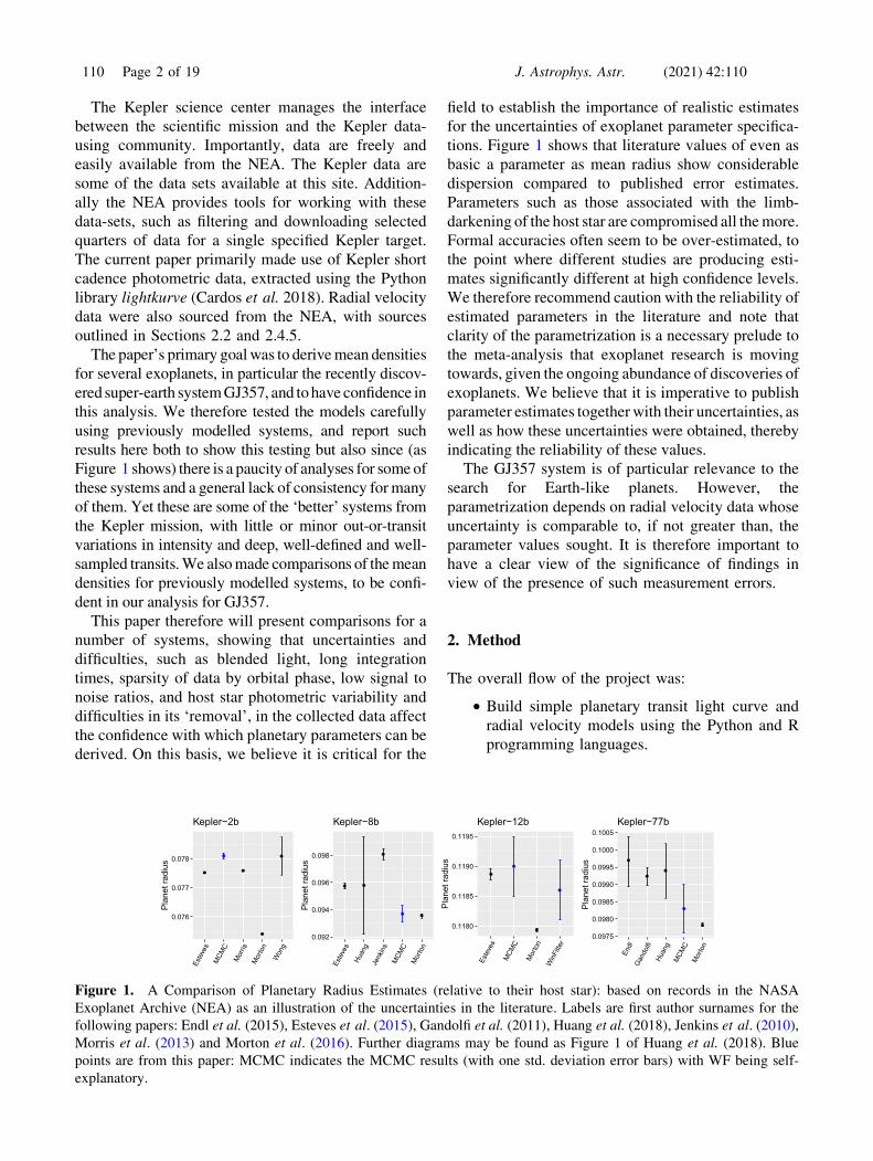
The paper’s primary goal was to derive mean densities

for several exoplanets, in particular the recently discov-

ered super-earth system GJ357, and to have confidence in

this analysis. We therefore tested the models carefully

using previously modelled systems, and report such

results here both to show this testing but also since (as

Figure 1 shows) there is a paucity of analyses for some of

these systems and a general lack of consistency for many

of them. Yet these are some of the ‘better’ systems from

the Kepler mission, with little or minor out-or-transit

variations in intensity and deep, well-defined and well-

sampled transits. We also made comparisons of the mean

densities for previously modelled systems, to be confi-

dent in our analysis for GJ357.

This paper therefore will present comparisons for a

number of systems, showing that uncertainties and

difficulties, such as blended light, long integration

times, sparsity of data by orbital phase, low signal to

noise ratios, and host star photometric variability and

difficulties in its ‘removal’, in the collected data affect

the confidence with which planetary parameters can be

derived. On this basis, we believe it is critical for the

field to establish the importance of realistic estimates

for the uncertainties of exoplanet parameter specifica-

tions. Figure 1 shows that literature values of even as

basic a parameter as mean radius show considerable

dispersion compared to published error estimates.

Parameters such as those associated with the limb-

darkening of the host star are compromised all the more.

Formal accuracies often seem to be over-estimated, to

the point where different studies are producing esti-

mates significantly different at high confidence levels.

We therefore recommend caution with the reliability of

estimated parameters in the literature and note that

clarity of the parametrization is a necessary prelude to

the meta-analysis that exoplanet research is moving

towards, given the ongoing abundance of discoveries of

exoplanets. We believe that it is imperative to publish

parameter estimates together with their uncertainties, as

well as how these uncertainties were obtained, thereby

indicating the reliability of these values.

The GJ357 system is of particular relevance to the

search for Earth-like planets. However, the

parametrization depends on radial velocity data whose

uncertainty is comparable to, if not greater than, the

parameter values sought. It is therefore important to

have a clear view of the significance of findings in

view of the presence of such measurement errors.

2. Method

The overall flow of the project was:

• Build simple planetary transit light curve and

radial velocity models using the Python and R

programming languages.

●

●

● ●

●

0.076

0.077

0.078

Este

ves

MCM

C

Mor

risM

orto

n

Won

g

Plan

et ra

dius

Kepler−2b

●

●

●

●

●

0.092

0.094

0.096

0.098

Este

ves

Huan

gJe

nkins

MCM

CM

orto

n

Plan

et ra

dius

Kepler−8b

●

●

●

●

0.1180

0.1185

0.1190

0.1195

Este

ves

MCM

C

Mor

ton

WinF

itter

Plan

et ra

dius

Kepler−12b

●

●

●

●

●

0.0975

0.0980

0.0985

0.0990

0.0995

0.1000

0.1005

Endl

Gand

olfi

Huan

gM

CMC

Mor

ton

Plan

et ra

dius

Kepler−77b

Figure 1. A Comparison of Planetary Radius Estimates (relative to their host star): based on records in the NASA

Exoplanet Archive (NEA) as an illustration of the uncertainties in the literature. Labels are first author surnames for the

following papers: Endl et al. (2015), Esteves et al. (2015), Gandolfi et al. (2011), Huang et al. (2018), Jenkins et al. (2010),

Morris et al. (2013) and Morton et al. (2016). Further diagrams may be found as Figure 1 of Huang et al. (2018). Blue

points are from this paper: MCMC indicates the MCMC results (with one std. deviation error bars) with WF being self-

explanatory.

110 of 19 J. Astrophys. Astr. (2021) 42:110

• Fit the models using simple optimizers, such as

the Levenberg–Marquadt algorithm.

• Apply more sophisticated modellers such as

WINFITTER (WF), comparing results from those

from the previous steps and with the literature,

to see if similar results were obtained. Should

there be good agreement, we would move on to

the next step.

• Employ Markov Chain Monte Carlo (MCMC)

procedures to obtain estimates and uncertainties

of the parameters for the systems.

• Derive density estimates for those systems with

both radial velocity and transit fits. Use the

more sophisticated EXOFAST modeller to fit

simultaneously the radial velocity and transit

data sets, and compare results.

Our goals were to build and test models, first using

synthetic data and then for systems with published

analyses, so that we could confirm that both the

models and the optimisation techniques were resulting

in reasonable estimates. This would lend confidence to

the later analyses, where we applied the more time-

consuming MCMC methodologies to estimate the

planetary densities for a number of systems. Publicly

available data were used in this study, sourced from

the literature, the MAST data archive at the Space

Telescope Science Institute (STScI), or the NEA. A

wide variety of modelling programs are used in the

exoplanet literature, making a comparison of all such

tools a substantial task. Instead, we selected several of

the more popular techniques for direct comparison in

this paper, together with comparisons of the literature

at the system level.

2.1 Initial models

A light curve model for photometric data and a radial

velocity model for spectroscopic data were built (in

Python) from first principles using Mandel & Agol’s

(2002) and Budding & Demircan’s (2007) formula-

tions for transit modelling, and Haswell (2010) and

Hatzes (2016) for the radial velocity models. Orbital

eccentricity was accounted for in the radial velocity

model and limb darkening laws (linear and quadratic)

were used in the photometric model. The ‘small pla-

net’ approximation was used for the transit model, in

that the limb darkening value/s corresponding to the

centre of the planetary disk projected onto the stellar

disk were uniformly applied across the stellar area

obscured by the planet. Heller (2019) reported that the

effect of this approximation is an order of magnitude

less that uncertainties arising from the total noise

budget in light curves, translating into typical errors in

the derived planetary radius (RP) of � 10�4 for RP ¼0:1 in highly accurate space-based observations of

bright stars (Gilliland et al. 2011) such as used in this

study. Heller noted that the approximation produces

errors which are orders of magnitude smaller than the

error coming from uncertain limb darkening coeffi-

cients. Croll et al. (2007) noted that the small planet

approximation is valid for ðRP=RSÞ\0:1, where RS is

the stellar radius. The systems we looked are generally

below this limit. However, two of the transit test cases

exceeded it and hence one explanation why we also

used more sophisticated models later in the paper.

2.2 Model tests

We checked whether the models give parameter esti-

mates in line with the literature. Two different opti-

misers (the Genetic and the Levenberg–Marquardt

(LM) algorithms) were applied to known exoplanetary

systems:

• Radial velocity data for 51 Peg-b, Kepler-12, -

14, -15 and -40. The 51 Peg data are from Butler

et al. (2006). Kepler-12 data are from Fortney

et al. Kepler-15 data are from Endl et al. (2011)

and Kepler-14 from Buchave et al. (2011). The

Kepler-14b fits below correspond to Buchave

et al.’s ‘uncorrected’ fit in that dilution of the

host star’s light by the nearly equal magnitude

stellar companion (�0.5 mag fainter) was not

taken into account. Kepler-40 data were taken

from Santerne et al. (2011).

• Photometric data from Kepler, sourced from the

NEA. Quarter 1 data was used for Kepler-1b.

For Kepler-2b, -12b and -13b, quarter 2 data

were extracted. Quarter 3 data were utilized for

Kepler-14b and -15b, whereas quarter 5 data

was used for Kepler-8b and -77b. We selected

quarters that, by visual inspection, minimised

out of transit variations in flux. We note that

Kepler-1b is also known as TrES-2b, being

discovered by O’Donovan et al. (2006). Most of

the systems chosen were selected because they

had no out-of-transit effects, for instance,

Kepler-1 has a uniform flux outside the transit

region. We did not analyse the entire three years

of Kepler data due to its volume and lack of

variation, besides these were essentially test

J. Astrophys. Astr. (2021) 42:110 of 19 110

cases to validate that the software was produc-

ing results in line with the literature. Two of the

systems (Kepler-14 and -77) exhibited waves

running through the out-of-transit data, which

we subsequently modelled using Gaussian pro-

cesses (GP) to ‘clean’ and remove these distur-

bances before the transits were modelled. A GP

is a collection of finite number random vari-

ables, which have a joint Gaussian distribution

(Rasmussen & Williams 2005). This means that

a GP can be completely determined by its mean

function and covariance function. In order to

remove the stellar variability in the transit, a GP

model is first fitted to the out-of-transit data and

then used for prediction. To facilitate a

smoother light curve fitting, we remove these

predictions from the original data, which

includes the transit data. We made use of the

Juliet package (Espinoza et al. 2019).

The LM algorithm can be seen as a combination of the

steepest gradient algorithm and the Newton algorithm

(Li et al. 2017). In this project, the LM algorithm is

implemented using the nls.lm function from the min-pack.lm package in R (Timur et al. 2016). LM gives

standard error estimates, although these formal errors

were clearly too small by several factors of ten. We

therefore do not report these errors as we place little

confidence in them, instead preferring to later use

Monte Carlo methods to make such estimates.

The R package genalg3 was used to implement the

genetic optimisations.

The other code we have applied for light curve

analysis is the graphical user interfaced close binary

system analysis program, WF. This program is

described in Rhodes & Budding (2014). It uses a

modified Levenberg–Marquardt optimisation tech-

nique to find the model light curve that corresponds to

the least value of v2. The fitting function is based on

the Radau formulations of Kopal (1959). These for-

mulations allow analysis of the tidal and rotational

distortions (ellipticity), together with the radiative

interactions (reflection), for massive and relatively

close gravitating bodies (a detailed background is

given by Budding et al. 2016a,b). WF has several

interesting points:

• The relatively simple and compact algebraic

form of the fitting function, which allows large

regions of the v2 parameter space to be explored

at low computing cost.

• The v2 Hessian (Bevington 1969) can be simply

evaluated in the vicinity of the derived minimum.

Inspecting this matrix, and in particular its eigen-

values and eigenvectors, gives valuable insights

into parameter determinacy and interdependence.

• The Hessian can be inverted to yield an error

matrix. This must be positive definite if a deter-

minate, ‘unique’ optimal solution is to be evalu-

ated. WF considers strict application of this

provision essential to avoid over-fitting the data.

The program uses three different optimisation

techniques:

1. Parabolic interpolation for single parameters, in a

step by step mode;

2. Parabolic in conjugate directions; and

3. Vector (in all parameters) mode.

The program switches between these modes depend-

ing on the convergence rate and user defined limits.

Further details on how WF addresses the information

content of data and estimation of uncertainties can be

found in Banks & Budding (1990).

The first step in optimisation used k, RS=a, i and uas free parameters, and then was followed by a second

step fixing these initial parameters to their derived

values and optimising for e and M0. Inclination is

denoted as i, k is the planet radius (RP) divided by the

stellar radius ðRSÞ, u is the linear limb darkening

value, and a is the semi-major axis of the exoplanets

orbit. The parameter errors were derived from the

Hessian inverse matrix calculated at the adopted

optimum. The formal error estimates are described in

detail by Budding et al. (2016b).

2.2.1 Radial velocity tests Table 1 lists the results

for the radial velocity fits, showing the LM fits to be in

general agreement with the papers modelling the same

data,4 and confirming the usefulness of this paper’s

simple model. The genetic algorithm tended to settle

on more divergent solutions, longer run times might

have lead to improvement through ‘wider’ searches.

Here, we note that the value for q and its associated

errors for 51 Peg could not be obtained from Bedell

et al. (2019) due to non-specification of M�. Addi-

tionally, an outlier ðBJD ¼ 2455019:11155; RV ¼36:7;rRV ¼ 19:4Þ was removed from data for

Kepler-12b before it was used for analysis. This was

done to minimise disruption of the sine wave structure

3https://github.com/egonw/genalg.

4Bar Butler et al. (2006) and Rosenthal et al. (2021) which were

included to confirm that other researchers had found indication of

eccentricity as well.


for the radial velocity model so that a better overall fit

could be obtained.

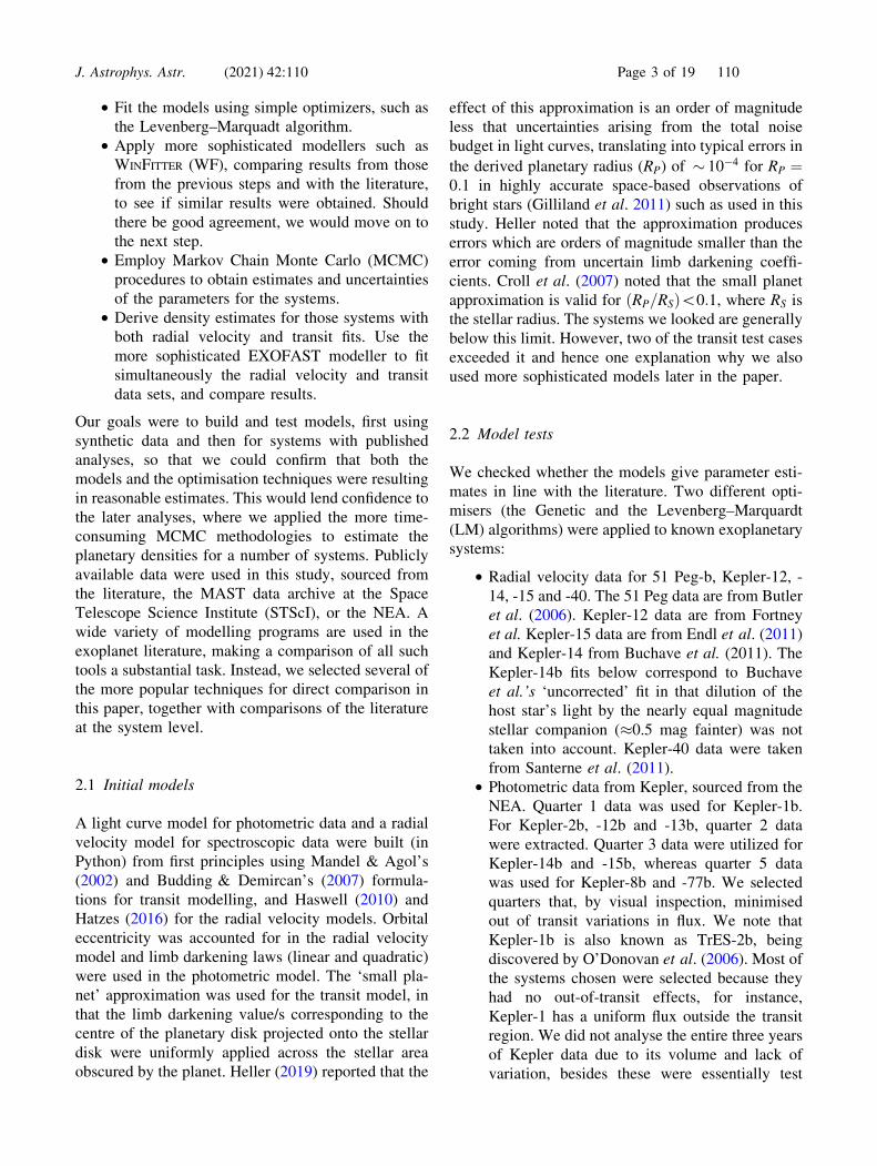
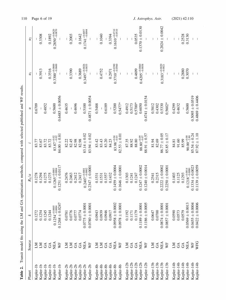
2.2.2 Transit tests Table 2 gives results for the

photometric modelling, showing again general

agreement across the different methods or sources

(see also Figure 2 which displays a comparison with

the NEA ‘preferred solutions’ across the systems). For

Kepler-13b, the model used to obtain these estimates

allowed eccentricity to be a free parameter. For all

other systems, eccentricity was fixed at 0. This is as

Kepler-13b is a system with complex effects which

are further explored in Budding et al. (2018). Such

treatment would give more reliable estimates since

lesser assumptions are made about the system,

although we acknowledge that it is a limited

representation of the effects present. In most fits,

only linear limb darkening could be constrained (u),

only in one fit for Kepler-13b were the quadratic

coefficients (u1 and u2) obtainable. WF refers to a

model fit using that program, and used Claret &

Bloemen (2011) to determine u (based on literature

information as given in Table 3). Formal errors are

not given in this table, but are discussed in the MCMC

fitting results. The goal of this section was to compare

point estimates for general agreement, given that the

GA could not produce error estimates and the formal

estimates from LM were too small to be realistic. The

NEA lines give both linear and quadratic coefficients.

The NEA radii and inclination values for Kepler-1b,

-2b, -8b, -12b and -13b are from Esteves et al. (2015),

-14b from Buchinave et al. (2011), -15b from Endl

et al. (2015), and -77b from Gandolfi et al. (2011). We

note in passing that Southworth’s (2012) values for

Kepler-14 are in better agreement with this study

than those of Buchinave et al. (2011). These are the

only two studies of the planet with inclinations

on NEA.

In general, the fits by this study were not able to

find viable solutions when quadratic limb darkening

was introduced as free variables, but could fit solu-

tions when linear limb darkening was included as a

free variable. This is to do with the information

content of the data, and is discussed by Ji et al.

Table 1. Comparison of point estimates from fitting of radial velocity data for 51 Peg-b, Kepler-12b, -14b, -15b and -40b.

System Method e RVC (km/s) q ð10�4Þ Semi-amplitude (m/s)

Kepler-12b LM 0.11 0.000 3.94 54.1

Kepler-12b GA 0.36 0.376 3.84 56.1

Kepler-12b Fortney 0:00þ0:01�0:01 0:0792þ0:0071

�0:0070 3:53þ0:52�0:46 48:2þ4:4

�4:3

Kepler-14b LM 0.03 2.490 32.4 404.4

Kepler-14b GA 0.09 1.671 32.6 409.0

Kepler-14b Buchave 0:035þ0:020�0:020 6:53þ0:30

�0:30 53:00þ3:83�3:55 682:9þ26:7

�24:6

Kepler-15b LM 0.16 24.02 6.35 83.5

Kepler-15b GA 0.26 18.95 6.38 85.7

Kepler-15b Endl – 20:0þ1:0�1:0 6:19þ1:12

�1:06 78:7þ8:5�9:5

Kepler-40b LM 0.00 6.591 17.0 220

Kepler-40b GA 0.14 6.582 7.0 100

Kepler-40b Santerne 0.00 (fixed) 6:565þ0:020�0:020 14:20þ3:29

�3:03 179þ27�27

51 Peg-b LM 0.021 0.000 4.30 56.6

51 Peg-b GA 0.021 0.295 4.04 53.1

51 Peg-b Bedell 0:03þ0:02�0:02

– – 55:57þ2:28�2:04

51 Peg-b Butler 0:013 � 0:12 – – 55:94 � 0:69

51 Peg-b Rosenthal 0:0042þ0:0046�0:0030

– – 55:73þ0:32�0:30

GA stands for results using the genetic optimisation method in this paper, and LM for results using the Levenberg–

Marquardt method. e is eccentricity, RVC is systemic velocity and q the mass ratio. The parameters are taken from the same

papers as the data. The 51 Peg data are from Butler et al. (2006), but the parameters given are from Bedell et al. (2019).

Papers are referred to by lead author name: Bedell et al. (2019), Buchave et al. (2011), Butler et al. (2006), Endl et al.(2011), Fortney et al. (2011), Rosenthal et al. (2021) and Santerne et al. (2011). The derived estimates from these studies

of the Kepler systems have been adopted as foundational by other researchers such as Southworth (2012) and Esteves et al.(2015), being the only papers modelling these radial velocity data. The NEA lists 5 papers with radial velocity solutions for

51 Peg, those selected had included eccentricity as a free parameter and so were directly comparable to the fit by this study.


Table

2.

Tra

nsi

tm

od

elfi

tsu

sin

gth

eL

Man

dG

Ao

pti

mis

atio

nm

eth

od

s,co

mp

ared

wit

hse

lect

edp

ub

lish

edan

dW

Fre

sult

s.

Pla

net

So

urc

ek

RS=

ai

uu

1u

2

Kep

ler-

1b

LM

0.1

27

20

.12

78

83

.77

0.6

70

9–

–

Kep

ler-

1b

LM

0.1

25

40

.12

94

83

.67

–0

.39

13

0.3

30

8

Kep

ler-

1b

GA

0.1

24

50

.12

75

83

.72

0.4

85

2–

–

Kep

ler-

1b

GA

0.1

24

40

.12

75

83

.72

–0

.35

16

0.1

89

2

Kep

ler-

1b

NE

A0:1

25

4þ

0:0

005

�0:0

004

0:1

26

5þ

0:0

003

�0:0

004

83:8

7þ

0:0

2�

0:0

20

.56

00

0:3

30

0þ

0:0

800

�0:0

600

0:2

85

0þ

0:0

620

�0:0

870

Kep

ler-

1b

WF

0:1

26

8�

0:0

24

70:1

25

1�

0:0

11

78

4:0

0�

0:8

10:6

48

5�

0:0

05

6–

–

Kep

ler-

2b

LM

0.0

78

10

.24

76

82

.22

0.4

63

5–

–

Kep

ler-

2b

LM

0.0

77

60

.24

63

82

.45

–0

.33

90

0.2

00

3

Kep

ler-

2b

GA

0.0

77

70

.24

12

82

.98

0.4

69

6–

–

Kep

ler-

2b

GA

0.0

77

40

.24

17

82

.98

–0

.36

89

0.1

64

2

Kep

ler-

2b

NE

A0:0

77

5�

0:0

00

10:2

40

7þ

0:0

001

�0:0

002

83:1

4�

0:0

20

.51

00

0:3

49

7þ

0:0

026

�0:0

035

0:1

74

1þ

0:0

057

�0:0

044

Kep

ler-

2b

WF

0:0

78

0�

0:0

00

10:2

34

7�

0:0

00

18

3:9

4�

0:0

20:4

87

1�

0:0

05

4–

–

Kep

ler-

8b

LM

0.0

94

30

.15

31

83

.42

0.5

48

8–

–

Kep

ler-

8b

LM

0.0

93

90

.15

31

83

.43

–0

.47

52

0.1

04

0

Kep

ler-

8b

GA

0.0

94

60

.15

57

83

.20

0.6

18

9–

–

Kep

ler-

8b

GA

0.0

91

70

.14

32

84

.23

–0

.29

71

0.3

39

4

Kep

ler-

8b

NE

A0:0

95

8�

0:0

00

20:1

45

9�

0:0

00

48

3:9

8þ

0:0

4�

0:0

30

.52

00

0:3

71

0þ

0:0

390

�0:0

560

0:1

61

0þ

0:0

710

�0:0

510

Kep

ler-

8b

WF

0:0

97

8�

0:0

00

10:1

64

6�

0:0

00

18

2:5

3�

0:0

10

.54

77

*–

–

Kep

ler-

12

bL

M0

.11

92

0.1

30

38

7.3

50

.49

12

––

Kep

ler-

12

bG

A0

.11

71

0.1

24

18

8.9

20

.51

73

––

Kep

ler-

12

bG

A0

.11

79

0.1

24

78

8.8

00

.57

00

*0

.46

99

0.0

53

5

Kep

ler-

12

bN

EA

0:1

18

9�

0:0

00

10:1

24

7�

0:0

00

28

8:8

0þ

0:0

9�

0:0

70

.60

50

0:4

20

5þ

0:0

060

�0:0

058

0:1

37

0�

0:0

13

0

Kep

ler-

12

bW

F0:1

18

6�

0:0

00

50:1

24

0�

0:0

01

48

8:9

1�

0:5

70:4

74

1�

0:0

15

4–

–

Kep

ler-

13

bL

M0

.06

47

0.2

54

18

1.9

40

.58

12

––

Kep

ler-

13

bG

A0

.07

00

0.2

31

58

2.6

90

.43

02

––

Kep

ler-

13

bN

EA

0:0

87

4�

0:0

00

10:2

22

2�

0:0

00

28

6:7

7�

0:0

50

.53

30

0:3

18

3þ

0:0

020

�0:0

021

0:2

02

4�

0:0

04

2

Kep

ler-

13

bW

F0:0

85

7�

0:0

00

10:2

25

0�

0:0

00

18

5:8

5�

0:1

70

.56

02

*–

–

Kep

ler-

14

bL

M0

.05

90

0.1

40

38

4.8

10

.42

99

––

Kep

ler-

14

bG

A0

.05

73

0.1

12

59

1.6

00

.46

32

––

Kep

ler-

14

bG

A0

.05

79

0.1

29

38

5.9

9–

0.2

88

00

.25

28

Kep

ler-

14

bN

EA

0:0

56

9�

0:0

01

30:1

21

8þ

0:0

014

�0:0

080

90:0

0þ

0:0

0�

2:8

00

.56

00

0.3

07

00

.31

30

Kep

ler-

14

bW

F0:0

45

5�

0:0

00

40:1

33

4�

0:0

02

38

5:5

4�

0:2

40:5

09

5�

0:0

51

9–

–

Kep

ler-

14

bW

FG

0:0

42

2�

0:0

00

60:1

13

9�

0:0

05

98

7:9

2�

1:1

00:4

86

9�

0:4

40

6–

–


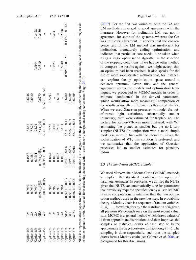
(2017). For the first two variables, both the GA and

LM methods converged to good agreement with the

literature. However for inclination LM was not in

agreement for some of the systems, whereas the GA

was in closer agreement. It appears that the conver-

gence test for the LM method was insufficient for

inclination, prematurely ending optimisation, and

indicates that particular care needs to be taken when

using a single optimisation algorithm in the selection

of the stopping conditions. If we had no other method

to compare the results against, we might accept that

an optimum had been reached. It also speaks for the

use of more sophisticated methods that, for instance,

can explore the v2 optimisation space around a

declared optimum. Given this, and the general

agreement across the models and optimisation tech-

niques, we proceeded to MCMC models in order to

estimate ‘confidence’ in the derived parameters,

which would allow more meaningful comparison of

the results across the difference methods and studies.

When we used Gaussian processes to model the out-

of-transit light variations, substantially smaller

(planetary) radii were estimated for Kepler-14b. The

picture for Kepler-77b was more confused, with WF

estimating the planet as smaller but the no-U-turn

sampler (NUTS) (in conjunction with a more simple

model) is more in line with the literature. Given the

sophistication of WF, this solution is preferred, and

we summarize that the application of Gaussian

processes led to smaller estimates for planetary

radius.

2.3 The no-U-turn MCMC sampler

We used Markov chain Monte Carlo (MCMC) methods

to explore the statistical confidence of optimized

parameter estimates. In particular, we utilised the NUTS

given that NUTS can automatically tune for parameters

that previously required specification by a user. MCMC

is more computationally intensive than the two optimi-

sation methods used in the previous step. In probability

theory, a Markov chain is a sequence of random variables

h1; h2; . . .; for which, for any t, the distribution ofht given

all previous h’s depends only on the most recent value,

ht�1. MCMC is a general method which draws values of

h from approximate distributions and then improves the

samples or statistical draws at each step to better

approximate the target posterior distribution, pðhjyÞ. The

sampling is done sequentially, such that the sampled

draws form a Markov chain (see Gelman et al. 2004, as

background for this discussion).Kep

ler-

15

bL

M0

.09

92

0.1

05

38

5.6

70

.62

46

––

Kep

ler-

15

bG

A0

.09

36

0.0

88

08

7.2

80

.66

30

––

Kep

ler-

15

bG

A0

.09

10

0.0

85

19

2.2

4–

0.5

19

40

.34

28

Kep

ler-

15

bN

EA

0:0

99

6þ

0:0

006

�0:0

005

0:0

78

1þ

0:0

104

�0:0

067

87:4

4þ

0:1

8�

0:2

00

.62

70

0.4

31

00

.24

30

Kep

ler-

15

bW

F0:1

00

8�

0:0

01

50:0

93

5�

0:0

03

86:8

0�

0:3

30:6

52

5�

0:0

58

6–

–

Kep

ler-

77

bL

M0

.09

83

0.1

04

48

7.6

30

.57

93

––

Kep

ler-

77

bL

M0

.09

60

0.1

02

38

8.1

8–

0.3

62

30

.48

41

Kep

ler-

77

bG

A0

.09

70

0.1

02

59

2.0

00

.62

10

––

Kep

ler-

77

bG

A0

.09

64

0.1

01

08

8.3

1–

0.5

04

00

.20

88

Kep

ler-

77

bN

EA

0:0

99

2�

0:0

00

30:1

02

4�

0:0

00

68

8:0

0�

0:1

10

.67

80

0:5

05

0�

0:0

15

00:1

39

0�

0:0

32

0

Kep

ler-

77

bW

F0:0

99

4�

0:0

00

30:1

01

9�

0:0

00

38

8:0

9�

0:0

50

.67

80

*–

–

Kep

ler-

77

bW

FG

0:0

96

8�

0:0

00

50:1

01

5�

0:0

01

88

6:1

4�

0:3

40

.67

80

*–

–

NE

Ais

are

pre

sen

tati

ve

pap

erfr

om

the

NE

Ata

ble

s.In

clin

atio

ni

isin

deg

rees

,k

isth

ep

lan

etra

diu

s(R

P)

div

ided

by

the

stel

lar

rad

ius

(RS)

and

ais

the

sem

i-m

ajo

rax

is

of

the

exo

pla

net

’so

rbit

.V

alu

eso

fli

mb

dar

ken

ing

den

ote

dw

ith�

wer

eli

nea

rly

inte

rpo

late

du

sin

gta

ble

sfr

om

Sin

g(2

01

0).


In our applications of Markov chain simulation,

several independent sequences are created. Each

sequence, h1; h2; h3; . . ., is produced by starting at some

point h0. Then, for each t, ht is drawn from a transition

distribution, Ttðhtjht�1Þ, which depends on the previous

draw ht�1. Each ht would contain N samples. The

transition probability distribution must be constructed

such that the Markov chain converges to a unique sta-

tionary distribution that is the target posterior

distribution, pðhjyÞ. Convergence was assessed using

the R statistic defined as (Gelman et al. 2004):

R ¼ffiffiffiffiffiffiffiffiffiffiffiffiffiffiffiffiffiffiffiffi

cvarþðwjyÞW

r

; ð1Þ

which declines to 1 as n ! 1. We note that:

cvarþðwjyÞ ¼ N � 1

NW þ 1

NB; ð2Þ

77b15b

14b

13b

12b

8b

2b

1b

0.07

0.09

0.11

0.07 0.09 0.11NLS k

NEA

k

Comparison between NEA and LM k

77b15b

14b

13b

12b

8b

2b

1b

0.07

0.09

0.11

0.07 0.09 0.11NLS k

NEA

k

Comparison between NEA and GA k

77b

15b

14b

13b

12b

8b

2b

1b

0.10

0.15

0.20

0.10 0.15 0.20 0.25LM Stellar Radius to a

NEA

Ste

llar R

adiu

s to

a

Comparison between NEA and LM Stellar Radius to semi−major axis

77b

15b

14b

13b

12b

8b

2b

1b

0.10

0.15

0.20

0.12 0.16 0.20 0.24GA Stellar Radius to a

NEA

Ste

llar R

adiu

s to

a

Comparison between NEA and GA Stellar Radius to semi−major axis

Figure 2. Comparison of genetic algorithm, LM and NEA results: the left hand column compares LM results with the

NEA-based figures for k and RS=a and the right column compares the same variables for the GA method with NEA-based

results. The green lines indicate where both methods plotted would be in agreement. These sample charts show the physical

ranges being tested across and the general agreement of the point estimates with the NEA-recommended values.

Table 3. Primary input data for transit curve fitting by WF.

System M� ðM�Þ R� ðR�Þ T� (K�) T 0eq (K�) u Epoch (BJD) P (days) References

Kepler-12 1.166 1.483 5947 1480 0.57 2455004.00915 4.4379629 Esteves et al. (2015)

Kepler-14 1.512 2.048 6395 1605 0.53 2454971.08737 6.7901230 Buchhave et al. (2011)

Kepler-15 1.018 0.992 5515 1251 0.64 2454969.328651 4.942782 Endl et al. (2011)


W and B refer to the between sample variance estimate

and within sample variance estimate respectively.

When the chains converge to a stationary distribution,

the R statistics will converge to 1. This is commonly

used as one of the criteria for assessing convergence in

MCMC algorithms.

Hoffman & Gelman (2014) explain the benefits of

NUTS succinctly that it ‘‘. . .uses a recursive algorithm

to build a set of likely candidate points that spans a

wide swath of the target distribution, stopping auto-

matically when it starts to double back and retrace its

steps. Empirically, NUTS performs at least as effi-

ciently as (and sometimes more efficiently than) a

well tuned standard HMC method, without requiring

user intervention or costly tuning runs.’’

We made use of STAN,5 which is a platform

accessible to popular data analysis languages such R,

Python, MATLAB, Julia and Stata. STAN provided us

with full Bayesian statistical inference with MCMC

sampling. It uses an approximate Hamiltonian

dynamics simulation based on numerical integration,

subsequently corrected by performing a Metropolis

acceptance step. The Hamiltonian Monte Carlo algo-

rithm starts at a specified initial set of parameters and

then across subsequent iterations, a new momentum

vector is sampled with the current values of the

parameters being updated using the leapfrog integrator

according to the Hamiltonian dynamics. A Metropolis

acceptance step is applied for each iteration, and a

decision is made whether to update to the new state or

keep the existing state.6

2.4 MCMC results

Having tested the model produced results in line with

the literature, we were ready to move through to

MCMC optimisation. Tables 4, 5 and 7 give the

NUTS results for the transit and radial velocity fits.

The application of Gaussian processes led to signifi-

cantly smaller estimates for the planetary radius of

Kepler-14b than in the literature, while the estimates

did not change significantly for Kepler-77b.

Before optimisation, we performed transformation

of some parameters for various reasons. By trans-

forming parameters RP, RS and a into ratios k ¼RP=RS and RS=a, we were able to reduce the

Table 4. MCMC transit model fits.

Planet k ð10�3Þ RS=a ð10�3Þ u cosðiÞ ð10�3Þ i (�)

Kepler-1b 126:8 � 0:3 127:7 � 0:3 0:648 � 0:025 108:4 � 0:4 83:77 � 0:02

Kepler-2b 78:1 � 0:1 247:3 � 1:2 0:468 � 0:005 134:5 � 2:3 82:27 � 0:13

Kepler-8b 93:7 � 0:6 148:8 � 3:3 0:513 � 0:043 108:8 � 0:5 83:75 � 0:03

Kepler-12b 119:0 � 0:5 129:1 � 1:5 0:495 � 0:005 42:1 � 0:5 87:59 � 0:03

Kepler-13b 65:6 � 0:1 310:8 � 6:1 0:461 � 0:007 227:9 � 10:2 76:83 � 0:60

Kepler-14b 57:9 � 0:6 133:2 � 6:3 0:465 � 0:033 77:2 � 11:4 85:57 � 0:66

Kepler-15b 99:6 � 0:4 106:7 � 1:3 0:610 � 0:024 77:9 � 1:9 85:53 � 0:11

Kepler-77b 98:3 � 0:7 107:0 � 0:2 0:565 � 0:021 48:5 � 0:5 87:22 � 0:03

Errors are one standard deviation. i is in degrees, k is the ratio of the planetary to stellar radius, RS is the

stellar radius and u is the linear limb darkening coefficient. Data were not yet corrected via Gaussian

processes for Kepler-14 and -77.

Table 5. MCMC transit model fits for data following subtraction of out of transit flux

variations, using Gaussian process models.

Planet k ð10�3Þ RS=a ð10�3Þ u cosðiÞ ð10�3Þ i (�)

Kepler-14b 46:8 � 0:3 148:8 � 5:0 0:477 � 0:027 102:5 � 7:4 84:12 � 0:43

Kepler-77b 98:6 � 0:5 104:5 � 1:6 0:579 � 0:140 41:4 � 0:4 87:37 � 0:25

Errors are one standard deviation. i is in degrees, k is the ratio of the planetary to stellar radius,

RS is the stellar radius and u is the linear limb darkening.

5See https://mc-stan.org/ more details. The STAN reference

manual is available at https://mc-stan.org/docs/2_25/reference-

manual/index.html.

6For further details on the algorithm and usage see https://mc-stan.

org/docs/2_25/reference-manual/hamiltonian-monte-carlo.html#

ref-Betancourt-Girolami:2013 and references within for further

details.


dimensionality of the optimisation problem. These

ratios and the limb darkening coefficients u, u1 and u2

take values between 0 and 1, which allows utilisation

of a uniform statistical prior distribution for sampling

draws in MCMC. Similarly, we transformed i into

cos i and used a uniform prior for the parameter. Such

a statistical prior would be ideal for obtaining an

unbiased estimate as we assume as little prior infor-

mation as possible for the optimised parameters.

Given the transformed parameters, the optimisation

problem to solve would be the following:

Lobserved �NðLfittedðphaseobserved;r2ÞÞ; ð3Þ

where Lfitted is the flux given by the final optimised

parameters and the observed phase and r is an indi-

cator of noise level in the data.

Figure 3 presents some illustrative transit model fits

across the test systems, along with the residuals to

those fits, while Table 4 lists the derived parameter

values and uncertainties from the fits. Overall, the

parameters are in reasonable agreement with those

listed from the earlier optimisations given in Table 2,

although there are some unexpected differences in the

inclination estimates for Kepler-12b and -13b. The

chains were well converged, as shown in Table 6.

Figure 4 shows an example scatter plot of the MCMC

results for the optimised parameters. Tables 7 and 8 list

the results for the MCMC fits to radial velocity data,

which showed good convergence. As can be seen, the

fits are reasonable (Figure 5) and in reasonable agree-

ment with the previous work given in Table 1.

2.4.1 Kepler-12b From these discussions, we were

able to calculate the densities for two planets, being

present in both the transit and radial velocity fits.

These are given in Table 9. The mean density for

Kepler-12b is similar to those estimates of 0.110 g per

cc of Bonomo et al. (2017), Esteves et al. (2015) and

Fortney et al. (2011) or 0.108 g per cc of Southworth

(2012), all of which gave errors of order 0.01. To

investigate further, we ran EXOFAST (Eastman et al.2013), which fits both the transit and radial velocity

data together using MCMC. As before, Quarter 2 data

were used from Kepler. For Kepler-12b, EXOFAST

derived a planetary mass of 0:44 � 0:04 MJ (Jupiter

masses), a radius of 1:72 � 0:05 RJ (Jupiter radii),

Table 6. MCMC transit model parameter R values.

Kepler-1b Kepler-2b Kepler-8b Kepler-12b Kepler-13b Kepler-14b Kepler-15b Kepler-77b

k 1.0001 1.0023 0.9997 1.0050 1.0008 1.0001 0.9999 0.9999

RS=a 1.0021 1.0007 1.0001 1.0049 1.0005 1.0002 0.9997 1.0003

u 1.0013 1.0000 0.9998 1.0021 0.9996 0.9996 1.0013 1.0002

cosðiÞ 1.0025 1.0009 1.0002 1.0060 1.0004 1.0004 0.9997 1.0004

●● ● ● ● ●●

●

●

●

●

●

●

●●

● ● ● ● ● ● ● ● ● ● ●●

●●

●

●

●

●

●

●● ● ● ● ● ● ●

0.990

0.995

1.000

0.48 0.49 0.50 0.51 0.52phase

flux

MCMC fitted flux for Kepler-1b

●

● ●

● ●

● ●●

●

●

●

●

●●

●●

●

●●

●

● ●

●

●

●●

●

●

●

●

●

●

●

●

●

●

●● ●

●

●

−1e−04

−5e−05

0e+00

5e−05

0.48 0.49 0.50 0.51 0.52phase

resi

dual

s

Residuals from MCMC for Kepler-1b

●●●●●●●●●●●●

●

●

●

●

●●●

●●●●●●●●●●●●●●●●●●●●●●●●●●●●●●●●●●●●●●●●●●●●●●●●●

●

●

●

●

●●●●●●●●●●●●

0.993

0.995

0.997

0.999

0.450 0.475 0.500 0.525 0.550phase

flux

MCMC fitted flux for Kepler-2b

●

●

●

●

●

●

●

●●

●

●

●

●

●

●

●

●●●

●

●

●●

●

●

●

●

●

●●

●●

●●

●

●

●

●●

●

●

●●●

●

●

●

●

●

●●●●●

●

●

●

●●

●●

●

●

●●

●●●

●●

●

●

●

●

●●●

●

●

●

●

●

●

●

−5e−05

0e+00

5e−05

1e−04

0.450 0.475 0.500 0.525 0.550phase

resi

dual

s

Residuals from MCMC for Kepler-2b

(a) (b)

Figure 3. Illustrative MCMC transit model fits and residuals for: (a) Kepler-1b and (b) -2b. For the point optimisations

we set 50 data points per bin and only looked at data that were near or in the transit. For the later MCMC fits (including

EXOFAST) we did not bin the data.


equilibrium temperature of 1490 � 30 K, inclination

of 88:8þ0:6�0:4 degrees, a Safronov number of

0:024 � 0:002, and a density of 0:11 � 0:01 g per

cc. All errors are one standard deviations. This density

is in better agreement with the literature. EXOFAST

derived a much more realistic eccentricity of

0:028þ0:04�0:02 than that above where the radial velocity

data were modelled without the transit data. The

derived mass ratio was 0:00035 � 0:00003, similar to

that from the earlier fit, but the planet radius was

slightly smaller at 0:1175þ0:0005�0:0004 relative to its star.

This might be due to the model using quadratic limb

darkening (coefficients 0:34 � 0:02 and 0:28 � 0:04)

compared to the linear term used in the previous

model. However, the overall agreement is reassuring.

2.4.2 Kepler-15b Turning to Kepler-15b, we also

ran EXOFAST on the same radial velocity data and

short cadence Quarter 3 Kepler data finding a solution

of 0:73 � 0:07 MJ , 1:040þ0:073�0:066 RJ , an equilibrium

temperature of 1135þ44�42 K, a Safronov number of

0:0768þ0:0098�0:0091, an ellipticity of 0:215þ0:070

�0:069, inclination

of 87:25þ0:26�0:31 degrees, a mass ratio of

0:00066 � 0:00006, and a mean density of 0:81þ0:19�0:16

g per cc. These results are generally close to the

STAN MCMC fit results (Table 9), which is again

reassuring. Quadratic limb darkening coefficients

were 0:45 � 0:04 and 0:21 � 0:05. The mean density

in the literature ranges from 0:404 � 0:048

(Southworth 2011) to 0:93þ0:18�0:22 (Bonomo et al.

2017), placing our density estimates in the upper

end of the range. The ellipticity appears unrealistic,

and so we reran EXOFAST forcing a circular orbit.

This led to a substantially lower mean estimated

density of 0:43 � 0:05 corresponding to final

estimates of 0:72 � 0:07 MJ , 1:27 � 0:04 RJ , a

substantially warmer equilibrium temperature of

1249 � 29 K, inclination of 86:15þ0:15�0:14 degrees, a

smaller Safronov number of 0:058 � 0:005, and a

similar mass ratio of 0:00060þ0:00005�0:00006. Limb darkening

coefficients were unchanged. The planetary radius

relative to its host star was larger than that estimated

from the STAN MCMC fit, at 0:0121 � 0:0006. These

results are in good agreement with those of

Southworth (2011). Additional radial velocity data

would likely lead to better constrained fits for the

sysytem.

2.4.3 Kepler-14b Kepler-14b proved to be a more

complex system than we had expected at the

beginning of the project. Bucchave et al. (2011)

found that the system was in a close visual binary

system. Our fitting (using Kepler Quarter 4 data) did

Table 7. MCMC radial velocity model fits.

Planet e q ð10�5Þ RVC

Kepler-12b 0:1594 � 0:0059 36:224 � 0:085 4:4167 � 0:1849

Kepler-14b 0:0373 � 0:0008 324:183 � 0:124 0:8351 � 0:1287

Kepler-15b 0:1852 � 0:0031 64:141 � 0:112 16:1181 � 0:1338

Kepler-40b 0:3193 � 0:0077 0:139 � 0:001 6:5500 � 0:0005

51 Peg-b 0:0188 � 0:0004 42:349 � 0:009 �2:4585 � 0:0099

Errors are one standard deviation. RVC is in km per second.

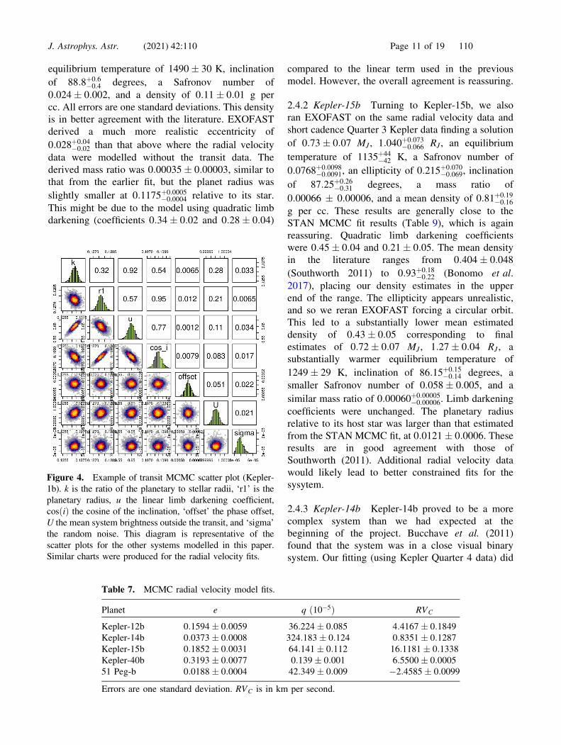
Figure 4. Example of transit MCMC scatter plot (Kepler-

1b). k is the ratio of the planetary to stellar radii, ‘r1’ is the

planetary radius, u the linear limb darkening coefficient,

cosðiÞ the cosine of the inclination, ‘offset’ the phase offset,

U the mean system brightness outside the transit, and ‘sigma’

the random noise. This diagram is representative of the

scatter plots for the other systems modelled in this paper.

Similar charts were produced for the radial velocity fits.


not take into account the dilution effect of the second

star, deriving a mean density of 13:9þ2:7�2:3 g per cc. This

is well outside the error limits of Bucchave et al. who

gave a mean density of 5:7þ1:5�1:0 before the dilution was

handled, and 7:1 � 1:1 afterwards. The large

eccentricity in our radial velocity fit is not likely to

be realistic, given the close orbit of the planet about its

host star. Given that our STAN MCMC fit did not

handle the dilution, we have not included our estimate

into Table 9. A first EXOFAST MCMC fit used the

undiluted data, deriving a mean density of 5:41þ0:59�0:51 g

per cc. This is still far from the STAN MCMC

estimate but in good agreement with Bucchave et al.In subsequent EXOFAST fits, diluting the flux by the

amount reported by Bucchave led to an estimated

mean density of 3:12þ0:35�0:31 g per cc, 4:95 � 0:17 MJ ,

1:25 � 0:05 RJ , an equilibrium temperature of 1596 �27 K, eccentricity at 0:023 � 0:013, a Safronov

number of 0:42 � 0:02, inclination of 86:2þ0:05�0:04

degrees, a mass ratio of 0:00315 � 0:00006, a

planetary radius of 0:0598 � 0:0004 its host star, and

a semi-major axis 8:0 � 0:2 the stellar radius. Limb

darkening values were 0:30 � 0:03 and 0:29 � 0:03

respectively. The orbital radius is larger than the

STAN estimates, and the density is not in agreement

with the value of Buchave et al. We suspected that

discrepancies could be due to the effect of ‘waves’

clearly running through the light curve. A Lomb–

Scargle (Lomb 1976; Scargle 1982; VanderPlas 2018)

analysis suggested periods of 6.1385, 5.6583 and

4.2557 days. We therefore ran EXOFAST over the

Table 8. MCMC radial velocity model

parameter R values.

Planet e q RVC

Kepler-12b 0.9998 1.0002 1.0011

Kepler-14b 1.0000 1.0006 0.9998

Kepler-15b 1.0000 0.9998 1.0000

Kepler-40b 0.9998 0.9997 1.0032

51 Peg-b 1.0029 0.9998 1.0005

●●

●●

●

●●

●

●

●

●

●

6.4

6.6

6.8

7.0

0e+00 2e+05 4e+05Phase

Rad

ial V

eloc

ity

MCMC fit for radial velocity of Kepler-40b

●●● ●

●

● ●

●

●

●

●

−0.05

0.00

0.05

0.10

0.15

1e+05 2e+05 3e+05 4e+05 5e+05Phase

Rad

ial V

eloc

ity

Residuals

(d)

−50

0

50

0.00 0.25 0.50 0.75 1.00Phase

Rad

ial V

eloc

ity

MCMC fit for radial velocity of Peg 51b

−20

−10

0

10

20

0.00 0.25 0.50 0.75 1.00Phase

Rad

ial V

eloc

ity

Residuals

(e)

−50

0

50

0.00 0.25 0.50 0.75 1.00Phase

Rad

ial V

eloc

ity


−20

0

20

40

60

0.2 0.4 0.6 0.8 1.0Phase

Rad

ial V

eloc

ity

Residuals

●●

● ● ●

●●●

●

●● ●

●●

−250

0

250

0e+00 2e+05 4e+05Phase

Rad

ial V

eloc

ity


●

●

●

●

●

●●

●

●

●●

●

●

●

−30−20−10

0102030

1e+05 2e+05 3e+05 4e+05 5e+05Phase

Rad

ial V

eloc

ity

Residuals

−100

0

100

0.00 0.25 0.50 0.75 1.00Phase

Rad

ial V

eloc

ity


−20

0

20

40

60

0.00 0.25 0.50 0.75 1.00Phase

Rad

ial V

eloc

ity

Residuals

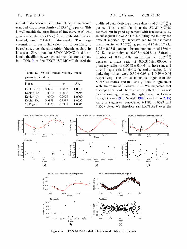
(a) (b) (c)

Figure 5. STAN MCMC radial velocity model fits and residuals.


Gaussian process corrected data used earlier, including

the dilution. A circular orbit was assumed from these

results. This led to an estimated density for the planet of

4:04 � 0:58, still lower than those of Bucchave, based

on a mass of 4:80þ0:18�0:17 MJ and 1:137þ0:069

�0:054 RJ . Such a

density suggests a rocky composition, perhaps similar to

Mars. Modelling the out-of-transit variations therefore

did not resolve the discrepancy. The other estimated

parameters were: effective temperature of 1537þ35�35,

Safronov number of 0:464þ0:024�0:027, orbital semi-major

axis (in stellar radii) of 8:66þ0:32�0:34, inclination of 88:0þ1:1

�0:8

degrees and a mass ratio of 0:00318 � 0:00007. Limb

darkening values were 0:271þ0:037�0:036 and 0:294þ0:046

�0:047

respectively. We are therefore unable to confirm the

densities given by Bucchave et al. (2011).

2.4.4 Kepler-40b For completeness, we ran

EXOFAST on Kepler-40b Quarter 5 Kepler long

cadence data and the radial velocity data used above.

A similar study of Kepler transit data by Huang et al.(2019) had discussed the biases introduced in modelling

long integration observations and so we were concerned

about these effects on our density estimate if we do not

consider the effect of long integration periods ‘blurring’

out photometric changes. Kipping (2010) also discussed

the problems involved in using long cadence Kepler

data, which EXOFAST has attempted to handle, as did

Santerne et al. when they investigated this planetary

system. We therefore used EXOFAST in preference to

our STAN methodology given its handling of long

integration periods.

A circular orbit was fixed (given the sparsity of the

radial velocity data), and the long cadence option used

in EXOFAST (which resamples the light curve 10

times uniformly spaced over the 29.5 min for each

Kepler long cadence data point and averaging). The

optimal solution was for a mass of 2:07 � 0:31 MJ , a

radius of 1:27þ0:18�0:07 RJ , a mean density of 1:19þ0:31

�0:36 g

per cc, an equilibrium temperature of 1662þ85�46, a

Safronov number of 0:16 � 0:03, inclination of

87:7þ1:5�1:9 degrees, a planet radius 0:0574þ0:0011

�0:0006 that of

its host star and a semi-major axis 7:73þ0:33�0:74 the stellar

radius. Quadratic limb darkening values were 0:26 �

0:04 and 0:30 � 0:05; respectively. These are generally

in reasonable agreement with the results of Santerne

et al. (2011), mainly due to the large uncertainties in

both results. For instance, Santerne et al. give the mean

planetary density as 1:68þ0:53�0:43 g per cc, also demon-

strating large uncertainties for this quantity.

Kepler-40b is a challenging system to fit, given the

accuracy of radial velocity data points (Kepler mag-

nitude 14:58 � 0:02) and long cadence photometry –

total transit duration is estimated at 0:2874þ0:0035�0:0024

days. So one data point is approximate 7% the dura-

tion of the transit. Given that the radial velocity data

were obtained with a small telescope (the 1.93-m at

Observatoire de Haute Province), it would be inter-

esting for a similar campaign using similar medium-

aperture telescopes to obtain further such data, which

would help firm up the modelling and subsequent

results. Similarly, further short integration period (but

low noise) photometry would be helpful.

2.4.5 GJ357 Photometric data from NASA’s

Transiting Exoplanet Survey Satellite (TESS) revealed

the Earth-like planet-containing exoplanet system

GJ357, as announced in mid-2019 (Luque et al. 2019).

GJ357’s M-type dwarf star, with mass of 0:342 � 0:011

M�, radius of 0:337 � 0:015 R� and � 0:015 of the

solar luminosity, hosts the interesting planet GJ357-b.

This was estimated to be about 20% larger than the

Earth, orbiting with a period of about 3.93 days, at a

separation from the star of about 0.033 AU.

With regard to representative values for the planet’s

mean surface temperatures TP, energy balance con-

siderations lead to the influx of energy Fin absorbed by

a planet of radius RP, given incident mean flux f0,

Bond albedo AB and cross-sectional area pR2P, being:

Fin ¼ f0ð1 � ABÞpR2P: ð4Þ

AB is zero for a ‘black body’, but from comparison

with the familiar cases of Venus and the Earth, 0.72

and 0.39 respectively (Allen 1973), we set a prior

value of AB as 0.5.

The radiation emitted from the (spherical) planet

Fout may then be associated with a representative

mean temperature TP, given by (Stefan’s law):

Fout ¼ 4pR2P�rT4

P; ð5Þ

where � is the emissivity, generally taken to be of

order unity, and r is Stefan’s constant. In a steady

state Fin ¼ Fout, and so

TP ¼ ðf0½1 � AB=4Þ1=4: ð6Þ

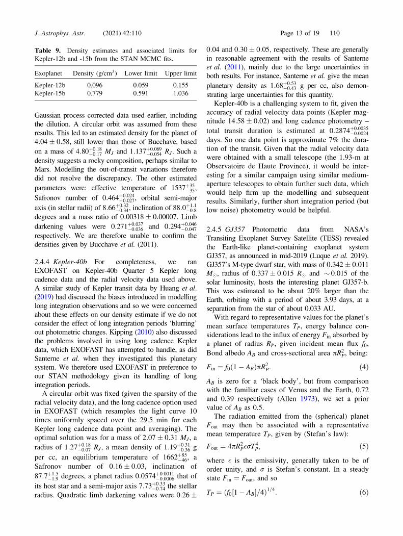
Table 9. Density estimates and associated limits for

Kepler-12b and -15b from the STAN MCMC fits.

Exoplanet Density (g/cm3) Lower limit Upper limit

Kepler-12b 0.096 0.059 0.155

Kepler-15b 0.779 0.591 1.036


Continuity of the stellar flux f0 from the source then

allows

TP � T�ð1 � ABÞ1=4

ffiffiffiffi

r1

2

r

; ð7Þ

where T� is the star’s effective surface temperature.

The average surface temperature estimated in this way

for GJ357-b is about 430 K. While GJ357-b thus lies

essentially outside the ‘habitable zone’ (HZ), the

object gains attention as the third-nearest transiting

exoplanet yet known, and potentially suitably arran-

ged for the study of rocky planet composition.

In the course of examination of supporting spec-

troscopic observations, Luque et al. (2019) found two

additional planetary candidates in the system. The

more separated of these (GJ357-d) orbits within the

HZ with a � 56 days period. Depending on its mass,

which is still not well-established, but estimated at

around 6 MEarth, GJ357-d could retain a sufficient

amount of atmosphere to support life-like biochemical

processes. The other planet, GJ357-c, has a mass of at

least 4 MEarth, orbital period of � 9.125 days, sepa-

ration of � 0.061 AU, and mean temperature that has

been estimated to be about 400 K, implying a low

Bond albedo. The object has not been confirmed

photometrically (nor has GJ357-d, which could be due

to their orbital inclinations not leading to transits),

though it should have been detected if its orbit were

within � 1:5� of 90�, which compares with � 88:5�

found for GJ357-b.

We also sourced TESS photometry for GJ357,

along with radial velocity data from the literature

following the interesting work of Luque et al. (2019).

While only one of these planet candidates transits, it

was classified as a ‘super-earth’, making it substan-

tially smaller than the other planets studied in this

paper and is an interesting challenge.

Firstly, we modelled these data using the STAN

MCMC methodology. Table 10 lists the MCMC

results for GJ357-b. While the chains are clearly

converged, the estimated errors are substantial (*5%

of k, 26% for the orbital radius, and nearly 3� from

maximum to minimum inclination). Limb darkening

was not surprisingly poorly estimated. WF estimates

given in Table 11 based on the same TESS data,

indicate a planet radius of R2 ¼ 1:18 � 0:02 R,

stellar radius of R1 ¼ 0:341 � 0:004 R�, and an

inclination of i ¼ 88:8 � 1:0 degrees, with an eccen-

tricity of e ¼ 0:278 � 0:053. WF prior information is

given in Table 12. The comparison between the

parameters estimated from the STAN MCMC fit

(Table 10) with those from WF are good, and also in

line with Luque et al. (2019).

WINFITTER can model radial velocity data, as well as

transit data. When we used all the radial velocity data

modelled by Luque et al., we were unable to calculate

a density for the transiting planet. We could neither

find a solution to the radial velocity data, nor could we

confirm the periods/existence of the two non-transit-

ing planets proposed by Luque et al. This was despite

realigning the subsets via their median or mean radial

velocities and following an iterative pre-whitening

and period analysis similar to that performed by

Luque et al. Neither WF nor STAN MCMC methods

could find determinate solutions. We therefore used

the derived (WF) planet radius and the mass from

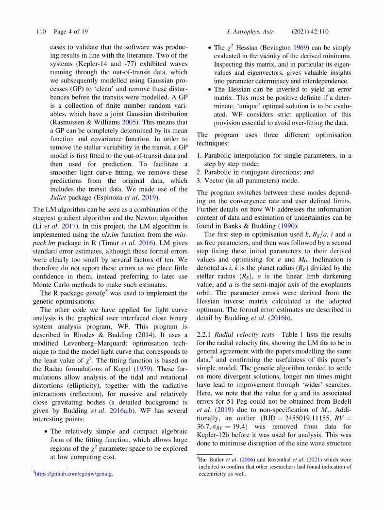
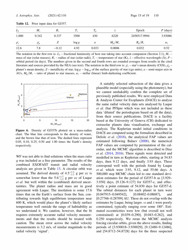
Luque et al. to calculate a bulk density of q ¼ 6:15 g

cm�3. This value would confirm GJ357-b as being an

Earth-like rocky planet, locating it between water and

iron density lines in a mass–radius diagram (Figure 6).

However, we were able to find a radial velocity

solution when we used a subset of those data, namely

the HIRES and UVES data sets and using EXOFAST.

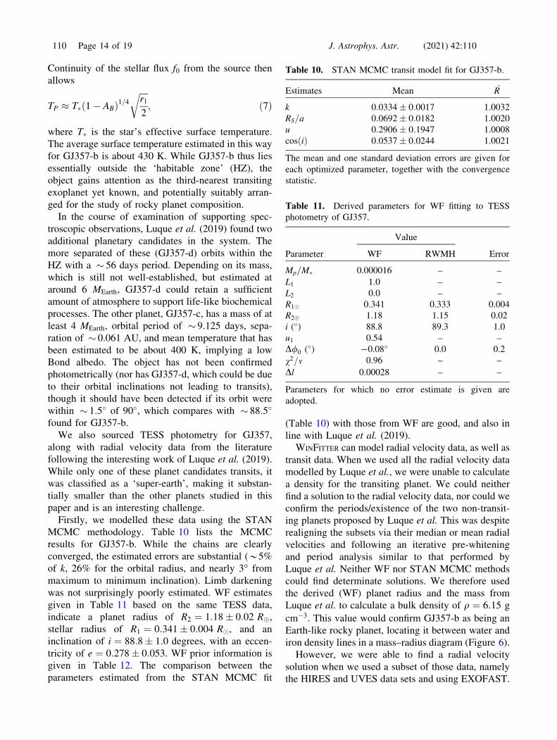
Table 10. STAN MCMC transit model fit for GJ357-b.

Estimates Mean R

k 0:0334 � 0:0017 1.0032

RS=a 0:0692 � 0:0182 1.0020

u 0:2906 � 0:1947 1.0008

cosðiÞ 0:0537 � 0:0244 1.0021

The mean and one standard deviation errors are given for

each optimized parameter, together with the convergence

statistic.

Table 11. Derived parameters for WF fitting to TESS

photometry of GJ357.

Value

Parameter WF RWMH Error

Mp=M� 0.000016 – –

L1 1.0 – –

L2 0.0 – –

R1� 0.341 0.333 0.004

R2 1.18 1.15 0.02

i (�) 88.8 89.3 1.0

u1 0.54 – –

D/0 (�) -0.08� 0.0 0.2

v2=m 0.96 – –

Dl 0.00028 – –

Parameters for which no error estimate is given are

adopted.


WF was not able to find solutions when the mass ratio

q was included as a free parameter. The results of the

combined EXOFAST transit and radial velocity

analysis are given in Table 13. A circular orbit was

assumed. The derived density of 4:5þ1:3�1:1 g per cc is

somewhat lower than the 5:6þ1:7�1:3 g per cc of Luque

et al. but well within the (combined) derived uncer-

tainties. The planet radius and mass are in good

agreement with Luque. The insolation is some 17.6

times that on the Earth’s surface from the Sun, con-

tributing towards high equilibrium temperature near

600 K, which would place the planet’s likely surface

temperature well outside the range of habitability as

we understand it. We caution, however, that the fit

requires extremely accurate radial velocity measure-

ments and that the results should be treated with

caution. The mean error across the radial velocity

measurements is 3.2 m/s, of similar magnitude to the

radial velocity ‘signal’.

A suitably selected subsection of the data gives a

plausible model (especially using the photometry), but

we cannot unshakably confirm the complete set of

previously published results. We next employed Data

& Analysis Center for Exoplanets (DACE) to analyse

the same radial velocity data sets analysed by Luque

et al. (bar PFSpre which was not included as these

data ‘diluted’ the periodogram based on all the data),

from their source publications. DACE is a facility

based at the University of Geneva (CH) dedicated to

extrasolar planets data visualisation, exchange and

analysis. The Keplerian model initial conditions in

DACE are computed using the formalism described in

Delisle et al. (2018), the analytical FAP values are

estimated following Baluev (2008), the numerical

FAP values are computed by permutation of the cal-

endar, and the MCMC algorithm is described in Diaz

et al. (2014, 2016). Three signals were detected and

modelled in turn as Keplerian orbits, starting at 54.83

days, then 9.12 days, and finally 3.93 days. These

correspond well with the periods found by Luque

et al. which were 3.93, 9.12, and 55.66 days. A

500,000 step MCMC chain led to one standard devi-

ation estimates for the period of GJ357-b as [3.929–

3.930] days, [9.126–9.127] for GJ357-c, and effec-

tively a point estimate of 54.830 days for GJ357-d.

The orbital distances for each planet in turn were

[0.047915–0.049542], [0.08402–0.08687], and

[0.27766–0.28709] AU. These do not overlap with the

estimates by Luque, being larger. x and k were poorly

constrained, typically ranging over some 180�. Esti-

mated eccentricities were low (but overall not well

constrained) at [0.039–0.290], [0.043–0.262], and

0.250 respectively. We reran the MCMC analysis

forcing circular orbits, given the above results, finding

periods of [3.930018–3.930029], [9.12480–9.12486],

and [54.8712–54.8728] days for the three suspected

Table 12. Prior input data for GJ357.

L1 M� R� T� Tp k Epoch P (days)

1.000 0.342 0.337 3500 430 6220 2458517.9994 3.93086

�q� �qp Z log g a Mp=M� Rp=R� u1

12.6 7.8 -0.12 4.92 0.033 0.0006 0.032 0.52

The notation in the first row is: L1 – fractional luminosity of host star taking into account companion (Section 2.1), M� –

mass of star (solar masses), R� – radius of star (solar radii), T� – temperature of star (K), k – effective wavelength (A), P –

orbital period (in days). The numbers given in the second and fourth rows are rounded averages from results in the cited

literature and sources provided by the NEA (see text). The notation in the third row is: �q� – star’s mean density (CGS), �qp –

planet’s mean density, Z – metallicity of star, log g � log10 of the surface gravity of star (cgs units), a – semi-major axis in

AUs, Mp=M� – ratio of planet to star masses, u1 – stellar (linear) limb-darkening coefficient.

Mars

Earth

UranusNeptune

GJ 357b

0

2

4

6

0 5 10 15 20M p (M earth)

Rp (R

earth

)

Figure 6. Density of GJ357b plotted on a mass-radius

chart. The blue line corresponds to the density of water,

and the brown line that of iron. The dashed lines represent

0.05, 0.10, 0.25, 0.50 and 1.00 times the Earth’s density

respectively.


planets, leading to mass estimates (m sin i) of [1.43–

1.74], [2.02–2.41], and [4.89–5.66] Earths respec-

tively. By comparison, Luque et al. give mass esti-

mates of 1:84þ0:31�0:31, [3:40þ0:46

�0:46, and [6:1þ1:0�1:0 Earth

masses. The orbital period for GJ357-d led to a pos-

sible transit for this ‘planet’ being outside the TESS

data collection period, while a possible transit for

GJ357-c was inside this period. We could not find this

transit in the photometric data. We did not have stellar

activity measures from the literature sources to be able

to distinguish such activity cycles from suspected

orbital periods. While we can confirm that there are

Table 13. EXOFAST median values and 68% confidence intervals for GJ357b.

Parameter Units Value

Stellar parametersM� Mass (M�) 0:514þ0:043

�0:042

R� Radius (R�) 0:377þ0:011�0:012

L� Luminosity (L�) 0:0275þ0:0046�0:0044

q� Density (cgs) 13:50þ0:63�0:60

logðg�Þ Surface gravity (cgs) 4:995 � 0:018

Teff Effective temperature (K) 3830þ110�120

½Fe=H Metalicity 0:02þ0:14�0:16

Planetary parametersP Period (days) 3:93048þ0:00014

�0:00015

a Semi-major axis (AU) 0:0390 � 0:0011

MP Mass (MJ) 0:0057þ0:0016�0:0013

RP Radius (RJ) 0:1164þ0:0044�0:0045

qP Density (cgs) 4:5þ1:3�1:1

logðgPÞ Surface gravity 3:02 � 0:11

Teq Equilibrium temperature (K) 573þ17�18

H Safronov number 0:0075þ0:0021�0:0017

hFi Incident flux (109 erg s�1 cm�2) 0:0246 � 0:0030

RV parametersK RV semi-amplitude (m/s) 1:15þ0:32

�0:26

MP sinðiÞ Minimum mass (MJ) 0:0057þ0:0016�0:0013

MP=M� Mass ratio 0:0000107þ0:0000030�0:0000024

c Systemic velocity (m/s) 0:76þ0:40�0:41

Primary transit parametersTC Time of transit (BJDTDB) 2458518:00039þ0:00071

�0:00059

RP=R� Radius of planet in stellar radii 0:03174þ0:00072�0:00074

a=R� Semi-major axis in stellar radii 22:25 � 0:34

u1 Linear limb-darkening coefficient 0:372 � 0:059

u2 quadratic limb-darkening coefficient 0:321þ0:056�0:057

i Inclination (�) 89:13þ0:14�0:13

b Impact parameter 0:336þ0:047�0:050

d Transit depth 0:001007 � 0:000046

TFWHM FWHM duration (days) 0:05295þ0:00075�0:00078

s Ingress/egress duration (days) 0:001896þ0:000083�0:000076

T14 Total duration (days) 0:05485þ0:00073�0:00077

PT A priori non-grazing transit probability 0:04351þ0:00067�0:00065

PT ;G A priori transit probability 0:04637þ0:00072�0:00070

F0 Baseline flux 1:000129 � 0:000017

Secondary eclipse parametersTS Time of eclipse (BJDTDB) 2458519:96563þ0:00065

�0:00054


three periods in the literature radial velocity data sets,

when they are ‘cleaned’ in the sequence given above,

further high accuracy data are needed to confirm the

two candidate planets (c and d). The DACE results are

tantalising but not conclusive, and further observa-

tions are clearly needed.

3. Discussion

We have built, from first principles simple models for

transit and radial velocity curve fitting, applying these

to a number of systems first using simple optimisation

techniques before moving to MCMC. Our findings are

in broad agreement with literature results. In the cases

of systems with both radial velocity and transit data,

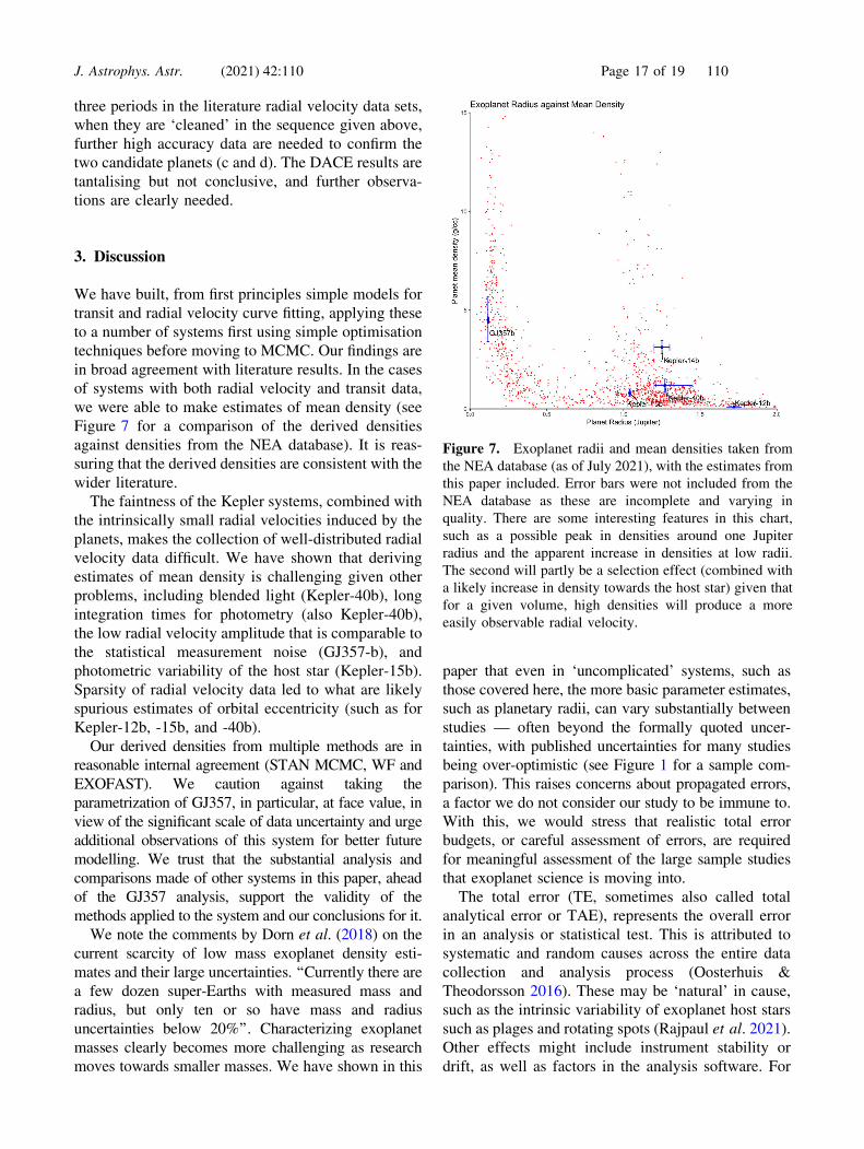
we were able to make estimates of mean density (see

Figure 7 for a comparison of the derived densities

against densities from the NEA database). It is reas-

suring that the derived densities are consistent with the

wider literature.

The faintness of the Kepler systems, combined with

the intrinsically small radial velocities induced by the

planets, makes the collection of well-distributed radial

velocity data difficult. We have shown that deriving

estimates of mean density is challenging given other

problems, including blended light (Kepler-40b), long

integration times for photometry (also Kepler-40b),

the low radial velocity amplitude that is comparable to

the statistical measurement noise (GJ357-b), and

photometric variability of the host star (Kepler-15b).

Sparsity of radial velocity data led to what are likely

spurious estimates of orbital eccentricity (such as for

Kepler-12b, -15b, and -40b).

Our derived densities from multiple methods are in

reasonable internal agreement (STAN MCMC, WF and

EXOFAST). We caution against taking the

parametrization of GJ357, in particular, at face value, in

view of the significant scale of data uncertainty and urge

additional observations of this system for better future

modelling. We trust that the substantial analysis and

comparisons made of other systems in this paper, ahead

of the GJ357 analysis, support the validity of the

methods applied to the system and our conclusions for it.

We note the comments by Dorn et al. (2018) on the

current scarcity of low mass exoplanet density esti-

mates and their large uncertainties. ‘‘Currently there are

a few dozen super-Earths with measured mass and

radius, but only ten or so have mass and radius

uncertainties below 20%’’. Characterizing exoplanet

masses clearly becomes more challenging as research

moves towards smaller masses. We have shown in this

paper that even in ‘uncomplicated’ systems, such as

those covered here, the more basic parameter estimates,

such as planetary radii, can vary substantially between

studies — often beyond the formally quoted uncer-

tainties, with published uncertainties for many studies

being over-optimistic (see Figure 1 for a sample com-

parison). This raises concerns about propagated errors,

a factor we do not consider our study to be immune to.

With this, we would stress that realistic total error

budgets, or careful assessment of errors, are required

for meaningful assessment of the large sample studies

that exoplanet science is moving into.

The total error (TE, sometimes also called total

analytical error or TAE), represents the overall error

in an analysis or statistical test. This is attributed to

systematic and random causes across the entire data

collection and analysis process (Oosterhuis &

Theodorsson 2016). These may be ‘natural’ in cause,

such as the intrinsic variability of exoplanet host stars

such as plages and rotating spots (Rajpaul et al. 2021).

Other effects might include instrument stability or

drift, as well as factors in the analysis software. For

Figure 7. Exoplanet radii and mean densities taken from

the NEA database (as of July 2021), with the estimates from

this paper included. Error bars were not included from the

NEA database as these are incomplete and varying in

quality. There are some interesting features in this chart,

such as a possible peak in densities around one Jupiter

radius and the apparent increase in densities at low radii.

The second will partly be a selection effect (combined with

a likely increase in density towards the host star) given that

for a given volume, high densities will produce a more

easily observable radial velocity.


instance, different limb-darkening ‘rules’ might be

employed; some models employ numerical methods to

model distortions (Wilson & Devinney 1971) while

others use algebric models (such as WF).

Many data analysis techniques applied to exoplan-

ets are based on the same formulae as those described

in this paper (such as the equations of Mandel & Agol

2002) and similar optimisation algorithms (such as

variants of MCMC) that contribute towards general

agreement between studies. However, between such

studies there are clearly also other factors leading to

the lack of full agreement (as shown Figure 1). We

would recommend carefully curating data and judi-

cious application of standard processes. We note that

the more advanced fitting functions used in this study

are in a broad agreement with the other methods.

However, the high quality of current and future data

require that we move from general to a formal

closeness of results with appropriate estimates of

fundamental parameters and their uncertainties.

Previously, the field of binary stars grappled with

similar issues to those faced by the exoplanet community

today, namely comparability of results using different

analysis techniques (Banks & Budding 1991) and treat-

ment of total errors. No single light curve model or

analysis technique was adopted by researchers, given the

overall philosophy that science advances through inde-

pendent confirmations. But there is agreement about

careful curation of data. This point is made in Torres

et al. (2010) painstaking examination of stellar masses

and radii based on 95 systems they assessed as being of

sufficient precision. Torres et al. recomputed the masses

and radii, using up-to-date physical constants, to ensure

uniformity of findings. This overall approach is desirable

for exoplanets parameters, given the increasing number

of studies and available results. Transparency on tech-

niques and methods in the source information is essential

for such meta-analyses. We would do well to emulate

Daniel Popper’s careful work on binary stars, referred to

in his obituary with ‘‘contrary to much astronomical

custom, Popper attached, generously realistic error bars

to his measurements, so that more recent redetermina-

tions have confirmed his early results more precisely than

could reasonably have been expected’’ (Trimble 1999).

We eagerly await the outcome of projects like

EXPRESS (Jurgenson et al. 2016) and EXPRESSO

(Hernandez et al. 2018) and the public release of their

data. This will allow independent follow-up studies

like this one, and hopefully reduce the ambiguities

shown here in exoplanet modelling via higher cadence

and precision radial velocities, leading to definitive,

curated studies as discussed above.

Acknowledgements

It is a pleasure to thank Prof. Osman Demircan and the

colleagues in the Physics Department of COMU

(Canakkale, Turkey) for their interest and support of

this programme. The research has been supported by

TUBITAK (Scientific and Technological Research

Council of Turkey) under Grant No. 113F353. This

paper includes data collected by the TESS Kepler

mission and obtained from the MAST data archive at

the Space Telescope Science Institute (STScI). Fund-

ing for the Kepler mission is provided by the NASA

Science Mission Directorate. STScI is operated by the

Association of Universities for Research in Astron-

omy, Inc., under NASA contract NAS 5–26555. This

research has made use of the NASA Exoplanet

Archive, which is operated by the California Institute

of Technology, under contract with the National

Aeronautics and Space Administration under the

Exoplanet Exploration Program; EXOFAST (Eastman

et al. 2013) as provided by the NASA Exoplanet

Archive; and Lightkurve, a Python package for Kepler

and TESS data analysis. The publication makes use of

the Data & Analysis Center for Exoplanets (DACE),

which is a facility based at the University of Geneva

(CH) dedicated to extrasolar planets data visualisa-

tion, exchange and analysis. DACE is a platform of

the Swiss National Centre of Competence in Research

(NCCR) PlanetS. The DACE platform is available at

https://dace.unige.ch. Additional help and encourage-

ment for this work has come from the National

University of Singapore (Ng 2019), particularly

through Prof. Lim Tiong Wee of the Department of

Statistics and Applied Probability. We thank the

University of Queensland for support via collabora-

tion software, and the anonymous referee for their

careful and helpful comments which improved this

paper.

References

Allen C. W. 1973, Astrophysical Quantities, Athlone Press,

University of London

Baluev R. V. 2008, MNRAS, 385, 1279

Banks T., Budding E. 1990, ApSS, 167, 221

Banks T., Budding E. 1991, Observatory, 111, 38

Bedell M., Hogg D. W., Foreman-Mackey D., Montet B.

T., Luger R. 2019, AJ, 158, 164

Bevington P. R. 1969, Data Reduction and Analysis for thePhysical Sciences, McGraw-Hill, New York

Bonomo A. S., Desidera S., Benatti S., et al. 2017, A&A,

602, 107


Borucki W. J., Koch D. G., Basri G. B., et al. 2003, in

Scientific Frontiers in Research on Extrasolar Planets,

Eds. Deming D., Seager S., ASP Conf. Ser. 294, 427

Borucki W. J., Koch D. G., Basri G., et al. 2011, ApJ, 736, 19

Buchhave L. A., Latham D. W., Carter J. A., et al. 2011,

ApJS, 197, 1

Budding E., Demircan O. 2007, Introduction to Astronom-ical Photometry, Cambridge University Press, ISBN:

978-0-521-84711-7

Budding E., Puskullu C., Rhodes M. D., Demircan O.,

Erdem A. 2016a, Ap&SS, 361, 17

Budding E., Rhodes M. D., Puskullu C., Ji Y., Erdem A.,

Banks T. 2016b, ApSS, 361, 346

Budding E., Puskullu C., Rhodes M. D. 2018, Ap&SS, 363, 60

Butler R. P., Wright J. T., Marcy G. W., et al. 2006, ApJ,

646, 505

Croll B., Matthews J. M., Rowe J. F., et al. 2007, ApJ, 658,

1328

Delisle J.-B, Segransan D., , Dumusque X., et al. 2018,

A&A, 614, A133

Diaz R. F., Almenara J. M., Santerne A., et al. 2014,

MNRAS, 441, 983

Diaz R. F., Segransan D., Udry S., et al. 2016, A&A, 585, A134

Dorn C., Bower D. J., Rozel A. 2018, in Deeg H., Belmonte

J. (eds), Handbook of Exoplanets, Springer, Cham,

https://doi.org/10.1007/978-3-319-55333-7_157, (see

also arxiv:1710.05605.pdf)

Eastman J., Gaudi B. S., Agol E. 2013, PASP, 125, 83

Endl M., MacQueen P. J., Cochran W. D., et al. 2011,

ApJS, 197, 13

Espinoza N., Kossakowski D., Brahm R. 2019, MNRAS,

490, 2262

Esteves L. J., De Mooij E. J. W., Jayawardhana R. 2015,

ApJ, 804, 150

Fortney J. J., Demory B.-O., Desert J.-M., et al. 2011,

ApJS, 197, 9

Gelman A., Carlin K., Stern H., Rubin D. 2004, BayesianData Analysis, Chapman & Hall, ISBN 0-412-03991-5

Gilliland R. L., Chaplin W. J., Dunham E. W., et al. 2011,

ApJS, 197, 6

Haswell C. 2010, Transiting Exoplanets, Cambridge

University Press, ISBN: 978-0-521-13938-0

Hatzes A. P. 2016, in Methods of Detecting Exoplanets: 1stAdvanced School on Exoplanetary Science, Eds: Bozza,

V, Mancini L., Sozzetti A., Springer, Astrophysics and

Space Science Library, p. 1, ISBN 978-3-319-27456-0

Heller R. 2019, A&A, 623, A137

Hernandez J. I. G., Pepe F., Molaro P., Santos N. C. 2018,

in Deeg H., Belmonte J. (eds) Handbook of Exoplanets,

Springer, Cham, https://doi.org/10.1007/978-3-319-

55333-7_157, p. 883

Hoffman M. D., Gelman A. 2014, Journal of Machine

Learning Research, 15, 1593.

Huang Q. Y., Banks T., Budding E., Puskullu C., Rhodes

M. D. 2019, ApSS, 364, 33

Jenkins J. M., Borucki W. J., Koch D. G., et al. 2010, ApJ,

724, 1108

Ji Y., Banks T., Budding E., Rhodes M. D. 2017, Ap&SS,

362, 12

Jurgenson C., Fischer D., McCracken T., et al. 2016,

SPIE.9908.6TJ, https://doi.org/10.1117/12.2233002

Kipping D. M. 2010, MNRAS, 408, 1758

Kopal Z. 1959, Close Binary Stars, The International

Astrophysics Series, London: Chapman & Hall

Lomb N. R. 1976, ApSS, 39, 447

Li J., Zheng W. X., Gu J., Hua L. 2017, Journal of the

Franklin Institute, 354, 316

Mandel K., Agol E. 2002, ApJ, 580, 171

Mayor M., Queloz D. 1995, Nature, 378, 355

Morris B. M., Mandell A. M., Deming D. 2013, ApJL, 764,

L22

Morton T. D., Bryson S. T., Coughlin J. L., et al. 2016,

ApJ, 822, 86, 15.

Ng S. Y. 2019, Unpublished Honours thesis, Dept.

Statistics & Applied Probability, National University of

Singapore

O’Donovan F. T., Charbonneau D., Mandushev G., et al.2006, ApJ, 651, L61

Oosterhuis W. P., Theodorsson E. 2016, Clin Chem Lab

Med, 54, 235

Rajpaul V. M., Buchhave L. A., Lacedelli G., et al. 2021,

arxiv:2107.13900

Rasmussen C. E., Williams C. K. I. 2005, GaussinProcesses for Machine Learning (Adaptive Computationand Machine Learning), MIT Press, Cambridge, USA

Rosenthal L. J, Fulton B. J., Hirsch L. A., et al. 2021, ApJS,

255, 8

Santerne A., Dıaz R. F., Bouchy F., et al. 2011, A&A, 528, 63

Scargle J. D. 1982, ApJ, 263, 835

Sing D. K. 2010, Astron. Astrophys., 510, A21

Southworth J. 2012, MNRAS, 426, 1291

Timur V. E., Katharine M. M., Andrej-Nikolai S., et al.2016, R Interface to the Levenberg-Marquardt NonlinearLeast-Squares Algorithm Found in MINPACK, PlusSupport for Bounds. Accessed December 21, 2019 from

https://cran.r-project.org/web/packages/minpack.lm

Torres G., Andersen J., Gimenez A. 2010, Astronomy and

Astrophysics Review, 18, 67

Trimble V., 1999, BAAS, 31. Retrieved from https://

baas.aas.org/pub/daniel-m-popper-1913-1999

VanderPlas J. T. 2018, ApJ Supl. Ser., 236, 16

Wilson R. E., Devinney E. J. 1971, ApJ, 166, 605


optimization applied to selected exoplanets

Documents