Optimization and Control

Contents

Table of Contents i

Schedules iv

1 Dynamic Programming 1

1.1 Control as optimization over time . . . . . . . . . . . . . . . . . . . . . . 1

1.2 The principle of optimality . . . . . . . . . . . . . . . . . . . . . . . . . 1

1.3 Example: the shortest path problem . . . . . . . . . . . . . . . . . . . . 1

1.4 The optimality equation . . . . . . . . . . . . . . . . . . . . . . . . . . . 2

1.5 Markov decision processes . . . . . . . . . . . . . . . . . . . . . . . . . . 4

2 Examples of Dynamic Programming 5

2.1 Example: optimization of consumption . . . . . . . . . . . . . . . . . . . 5

2.2 Example: exercising a stock option . . . . . . . . . . . . . . . . . . . . . 6

2.3 Example: secretary problem . . . . . . . . . . . . . . . . . . . . . . . . . 7

3 Dynamic Programming over the Infinite Horizon 9

3.1 Discounted costs . . . . . . . . . . . . . . . . . . . . . . . . . . . . . . . 9

3.2 Example: job scheduling . . . . . . . . . . . . . . . . . . . . . . . . . . . 9

3.3 The infinite-horizon case . . . . . . . . . . . . . . . . . . . . . . . . . . . 10

3.4 The optimality equation in the infinite-horizon case . . . . . . . . . . . . 11

3.5 Example: selling an asset . . . . . . . . . . . . . . . . . . . . . . . . . . 12

4 Positive Programming 13

4.1 Example: possible lack of an optimal policy. . . . . . . . . . . . . . . . . 13

4.2 Characterization of the optimal policy . . . . . . . . . . . . . . . . . . . 13

4.3 Example: optimal gambling . . . . . . . . . . . . . . . . . . . . . . . . . 14

4.4 Value iteration . . . . . . . . . . . . . . . . . . . . . . . . . . . . . . . . 14

4.5 Example: pharmaceutical trials . . . . . . . . . . . . . . . . . . . . . . . 15

5 Negative Programming 17

5.1 Example: a partially observed MDP . . . . . . . . . . . . . . . . . . . . 17

5.2 Stationary policies . . . . . . . . . . . . . . . . . . . . . . . . . . . . . . 18

5.3 Characterization of the optimal policy . . . . . . . . . . . . . . . . . . . 18

5.4 Optimal stopping over a finite horizon . . . . . . . . . . . . . . . . . . . 19

5.5 Example: optimal parking . . . . . . . . . . . . . . . . . . . . . . . . . . 20

i

6 Optimal Stopping Problems 21

6.1 Bruss’s odds algorithm . . . . . . . . . . . . . . . . . . . . . . . . . . . . 21

6.2 Example: Stopping a random walk . . . . . . . . . . . . . . . . . . . . . 22

6.3 Optimal stopping over the infinite horizon . . . . . . . . . . . . . . . . . 22

6.4 Sequential Probability Ratio Test . . . . . . . . . . . . . . . . . . . . . . 24

6.5 Bandit processes . . . . . . . . . . . . . . . . . . . . . . . . . . . . . . . 24

7 Bandit Processes and the Gittins Index 25

7.1 Multi-armed bandit problem . . . . . . . . . . . . . . . . . . . . . . . . 25

7.2 The two-armed bandit . . . . . . . . . . . . . . . . . . . . . . . . . . . . 26

7.3 Gittins index theorem . . . . . . . . . . . . . . . . . . . . . . . . . . . . 26

7.4 Playing golf with many balls . . . . . . . . . . . . . . . . . . . . . . . . 27

7.5 Example: Weitzman’s problem . . . . . . . . . . . . . . . . . . . . . . . 28

7.6 *Calculation of the Gittins index* . . . . . . . . . . . . . . . . . . . . . 29

7.7 *Forward induction policies* . . . . . . . . . . . . . . . . . . . . . . . . 29

7.8 *Proof of the Gittins index theorem* . . . . . . . . . . . . . . . . . . . . 29

8 Average-cost Programming 31

8.1 Average-cost optimality equation . . . . . . . . . . . . . . . . . . . . . . 31

8.2 Example: admission control at a queue . . . . . . . . . . . . . . . . . . . 32

8.3 Value iteration bounds . . . . . . . . . . . . . . . . . . . . . . . . . . . . 32

8.4 Policy improvement algorithm . . . . . . . . . . . . . . . . . . . . . . . . 33

9 Continuous-time Markov Decision Processes 35

9.1 Stochastic scheduling on parallel machines . . . . . . . . . . . . . . . . . 35

9.2 Controlled Markov jump processes . . . . . . . . . . . . . . . . . . . . . 37

9.3 Example: admission control at a queue . . . . . . . . . . . . . . . . . . . 38

10 LQ Regulation 40

10.1 The LQ regulation problem . . . . . . . . . . . . . . . . . . . . . . . . . 40

10.2 The Riccati recursion . . . . . . . . . . . . . . . . . . . . . . . . . . . . . 42

10.3 White noise disturbances . . . . . . . . . . . . . . . . . . . . . . . . . . 42

10.4 LQ regulation in continuous-time . . . . . . . . . . . . . . . . . . . . . . 43

10.5 Linearization of nonlinear models . . . . . . . . . . . . . . . . . . . . . . 43

11 Controllability and Observability 44

11.1 Controllability and Observability . . . . . . . . . . . . . . . . . . . . . . 44

11.2 Controllability . . . . . . . . . . . . . . . . . . . . . . . . . . . . . . . . 44

11.3 Controllability in continuous-time . . . . . . . . . . . . . . . . . . . . . . 46

11.4 Example: broom balancing . . . . . . . . . . . . . . . . . . . . . . . . . 46

11.5 Stabilizability . . . . . . . . . . . . . . . . . . . . . . . . . . . . . . . . . 47

11.6 Example: pendulum . . . . . . . . . . . . . . . . . . . . . . . . . . . . . 47

11.7 Example: satellite in a plane orbit . . . . . . . . . . . . . . . . . . . . . 48

ii

12 Observability and the LQG Model 4912.1 Infinite horizon limits . . . . . . . . . . . . . . . . . . . . . . . . . . . . 4912.2 Observability . . . . . . . . . . . . . . . . . . . . . . . . . . . . . . . . . 4912.3 Observability in continuous-time . . . . . . . . . . . . . . . . . . . . . . 5112.4 Example: satellite in planar orbit . . . . . . . . . . . . . . . . . . . . . . 5112.5 Imperfect state observation with noise . . . . . . . . . . . . . . . . . . . 51

13 Kalman Filter and Certainty Equivalence 5313.1 The Kalman filter . . . . . . . . . . . . . . . . . . . . . . . . . . . . . . 5313.2 Certainty equivalence . . . . . . . . . . . . . . . . . . . . . . . . . . . . . 5413.3 The Hamilton-Jacobi-Bellman equation . . . . . . . . . . . . . . . . . . 5513.4 Example: LQ regulation . . . . . . . . . . . . . . . . . . . . . . . . . . . 5613.5 Example: harvesting fish . . . . . . . . . . . . . . . . . . . . . . . . . . . 57

14 Pontryagin’s Maximum Principle 6014.1 Example: optimization of consumption . . . . . . . . . . . . . . . . . . . 6014.2 Heuristic derivation of Pontryagin’s maximum principle . . . . . . . . . 6114.3 Example: parking a rocket car . . . . . . . . . . . . . . . . . . . . . . . 6214.4 Adjoint variables as Lagrange multipliers . . . . . . . . . . . . . . . . . 64

15 Using Pontryagin’s Maximum Principle 6515.1 Transversality conditions . . . . . . . . . . . . . . . . . . . . . . . . . . . 6515.2 Example: use of transversality conditions . . . . . . . . . . . . . . . . . 6515.3 Example: insects as optimizers . . . . . . . . . . . . . . . . . . . . . . . 6615.4 Problems in which time appears explicitly . . . . . . . . . . . . . . . . . 6615.5 Example: monopolist . . . . . . . . . . . . . . . . . . . . . . . . . . . . . 6715.6 Example: neoclassical economic growth . . . . . . . . . . . . . . . . . . 68

16 Controlled Diffusion Processes 7016.1 The dynamic programming equation . . . . . . . . . . . . . . . . . . . . 7016.2 Diffusion processes and controlled diffusion processes . . . . . . . . . . . 7016.3 Example: noisy LQ regulation in continuous time . . . . . . . . . . . . . 7116.4 Example: passage to a stopping set . . . . . . . . . . . . . . . . . . . . . 72

iii

Schedules

Dynamic programmingThe principle of optimality. The dynamic programming equation for finite-horizonproblems. Interchange arguments. Markov decision processes in discrete time. Innite-horizon problems: positive, negative and discounted cases. Value interation. Policyimprovement algorithm. Stopping problems. Average-cost programming. [6]

LQG systemsLinear dynamics, quadratic costs, Gaussian noise. The Riccati recursion. Controlla-bility. Stabilizability. Innite-horizon LQ regulation. Observability. Imperfect stateobservation and the Kalman lter. Certainty equivalence control. [5]

Continuous-time modelsThe optimality equation in continuous time. Pontryagins maximum principle. Heuristicproof and connection with Lagrangian methods. Transversality conditions. Optimalityequations for Markov jump processes and diffusion processes. [5]

Richard Weber, January 2013

iv

1 Dynamic Programming

Dynamic programming and the principle of optimality. Notation for state-structured models.

Feedback, open-loop, and closed-loop controls. Markov decision processes.

1.1 Control as optimization over time

Optimization is a key tool in modelling. Sometimes it is important to solve a problemoptimally. Other times either a near-optimal solution is good enough, or the realproblem does not have a single criterion by which a solution can be judged. However,even when an optimal solution is not required it can be useful to test one’s thinkingby following an optimization approach. If the ‘optimal’ solution is ridiculous it maysuggest ways in which both modelling and thinking can be refined.

Control theory is concerned with dynamic systems and their optimization overtime. It accounts for the fact that a dynamic system may evolve stochastically andthat key variables may be unknown or imperfectly observed.

The optimization models in the IB course (for linear programming and networkflow models) were static and nothing was either random or hidden. In this courseit is the additional features of dynamic and stochastic evolution, and imperfect stateobservation, that give rise to new types of optimization problem and which require newways of thinking.

We could spend an entire lecture discussing the importance of control theory andtracing its development through the windmill, steam governor, and so on. Such ‘classiccontrol theory’ is largely concerned with the question of stability, and there is much ofthis theory which we ignore, e.g., Nyquist criterion and dynamic lags.

1.2 The principle of optimality

A key idea in this course is that optimization over time can often be seen as ‘optimiza-tion in stages’. We trade off our desire to obtain the least possible cost at the presentstage against the implication this would have for costs at future stages. The best actionminimizes the sum of the cost incurred at the current stage and the least total costthat can be incurred from all subsequent stages, consequent on this decision. This isknown as the Principle of Optimality.

Definition 1.1 (Principle of Optimality). From any point on an optimal trajectory,the remaining trajectory is optimal for the problem initiated at that point.

1.3 Example: the shortest path problem

Consider the ‘stagecoach problem’ in which a traveller wishes to minimize the lengthof a journey from town A to town J by first travelling to one of B, C or D and thenonwards to one of E, F or G then onwards to one of H or I and the finally to J. Thusthere are 4 ‘stages’. The arcs are marked with distances between towns.

1

A

B

C

D

E

F

G

H

I

J

1

1

2

2

3

3

3

33

3

4

4

4

4

4

4

5

6

6

7

Road system for stagecoach problem

Solution. Let F (X) be the minimal distance required to reach J from X. Then clearly,F (J) = 0, F (H) = 3 and F (I) = 4.

F (F) = min[ 6 + F (H), 3 + F (I) ] = 7,

and so on. Recursively, we obtain F (A) = 11 and simultaneously an optimal route, i.e.A→D→F→I→J (although it is not unique).

The study of dynamic programming dates from Richard Bellman, who wrote thefirst book on the subject (1957) and gave it its name. A very large number of problemscan be treated this way.

1.4 The optimality equation

The optimality equation in the general case. In discrete-time t takes integervalues, say t = 0, 1, . . . . Suppose ut is a control variable whose value is to be chosen attime t. Let Ut−1 = (u0, . . . , ut−1) denote the partial sequence of controls (or decisions)taken over the first t stages. Suppose the cost up to the time horizon h is given by

C = G(Uh−1) = G(u0, u1, . . . , uh−1).

Then the principle of optimality is expressed in the following theorem.

Theorem 1.2 (The principle of optimality). Define the functions

G(Ut−1, t) = infut,ut+1,...,uh−1

G(Uh−1).

Then these obey the recursion

G(Ut−1, t) = infut

G(Ut, t+ 1) t < h,

with terminal evaluation G(Uh−1, h) = G(Uh−1).

The proof is immediate from the definition of G(Ut−1, t), i.e.

G(Ut−1, t) = infut

{

infut+1,...,uh−1

G(u0, . . . , ut−1, ut , ut+1, . . . , uh−1)

}

.

2

The state structured case. The control variable ut is chosen on the basis of knowingUt−1 = (u0, . . . , ut−1), (which determines everything else). But a more economicalrepresentation of the past history is often sufficient. For example, we may not need toknow the entire path that has been followed up to time t, but only the place to whichit has taken us. The idea of a state variable x ∈ R

d is that its value at t, denoted xt,can be found from known quantities and obeys a plant equation (or law of motion)

xt+1 = a(xt, ut, t).

Suppose we wish to minimize a separable cost function of the form

C =

h−1∑

t=0

c(xt, ut, t) +Ch(xh), (1.1)

by choice of controls {u0, . . . , uh−1}. Define the cost from time t onwards as,

Ct =

h−1∑

τ=t

c(xτ , uτ , τ) +Ch(xh), (1.2)

and the minimal cost from time t onwards as an optimization over {ut, . . . , uh−1}conditional on xt = x,

F (x, t) = infut,...,uh−1

Ct.

Here F (x, t) is the minimal future cost from time t onward, given that the state is x attime t. Then by an inductive proof, one can show as in Theorem 1.2 that

F (x, t) = infu[c(x, u, t) + F (a(x, u, t), t+ 1)], t < h, (1.3)

with terminal condition F (x, h) = Ch(x). Here x is a generic value of xt. The mini-mizing u in (1.3) is the optimal control u(x, t) and values of x0, . . . , xt−1 are irrelevant.The optimality equation (1.3) is also called the dynamic programming equation(DP) or Bellman equation.

The DP equation defines an optimal control problem in what is called feedback orclosed-loop form, with ut = u(xt, t). This is in contrast to the open-loop formulationin which {u0, . . . , uh−1} are to be determined all at once at time 0. A policy (orstrategy) is a rule for choosing the value of the control variable under all possiblecircumstances as a function of the perceived circumstances. To summarise:

(i) The optimal ut is a function only of xt and t, i.e. ut = u(xt, t).

(ii) The DP equation expresses the optimal ut in closed-loop form. It is optimalwhatever the past control policy may have been.

(iii) The DP equation is a backward recursion in time (from which we get the optimumat h− 1, then h− 2 and so on.) The later policy is decided first.

‘Life must be lived forward and understood backwards.’ (Kierkegaard)

3

1.5 Markov decision processes

Consider now stochastic evolution. Let Xt = (x0, . . . , xt) and Ut = (u0, . . . , ut) denotethe x and u histories at time t. As above, state structure is characterised by the factthat the evolution of the process is described by a state variable x, having value xt attime t. The following assumptions define what is known as a discrete-time Markovdecision process (MDP).

(a) Markov dynamics: (i.e. the stochastic version of the plant equation.)

P (xt+1 | Xt, Ut) = P (xt+1 | xt, ut).

(b) Separable (or decomposable) cost function, (i.e. cost given by (1.1)).

For the moment we also require the following:

(c) Perfect state observation: The current value of the state is observable. That is, xt

is known when choosing ut. So, letting Wt denote the observed history at time t,we assume Wt = (Xt, Ut−1).

Note that C is determined by Wh, so we might write C = C(Wh).

As in the previous section, the cost from time t onwards is given by (1.2). Denotethe minimal expected cost from time t onwards by

F (Wt) = infπ

Eπ[Ct | Wt],

where π denotes a policy, i.e. a rule for choosing the controls u0, . . . , uh−1.The following theorem is then obvious.

Theorem 1.3. F (Wt) is a function of xt and t alone, say F (xt, t). It obeys theoptimality equation

F (xt, t) = infut

{c(xt, ut, t) + E[F (xt+1, t+ 1) | xt, ut]} , t < h, (1.4)

with terminal conditionF (xh, h) = Ch(xh).

Moreover, a minimizing value of ut in (1.4) (which is also only a function xt and t) isoptimal.

Proof. The value of F (Wh) is Ch(xh), so the asserted reduction of F is valid at timeh. Assume it is valid at time t+ 1. The DP equation is then

F (Wt) = infut

{c(xt, ut, t) + E[F (xt+1, t+ 1) | Xt, Ut]}. (1.5)

But, by assumption (a), the right-hand side of (1.5) reduces to the right-hand memberof (1.4). All the assertions then follow.

4

2 Examples of Dynamic Programming

Examples of dynamic programming problems and some useful tricks to solve them. The idea

that it can be useful to model things in terms of time to go.

2.1 Example: optimization of consumption

An investor receives annual income of xt pounds in year t. He consumes ut and addsxt − ut to his capital, 0 ≤ ut ≤ xt. The capital is invested at interest rate θ × 100%,and so his income in year t+ 1 increases to

xt+1 = a(xt, ut) = xt + θ(xt − ut). (2.1)

He desires to maximize total consumption over h years,

C =

h−1∑

t=0

c(xt, ut, t) +Ch(xh) =

h−1∑

t=0

ut

The plant equation (2.1) specifies a Markov decision process (MDP). Whenwe add to this the aim of maximizing the performance measure C we have what iscalled a Markov decision problem. For both we use the abbreviation MDP. In thenotation we have been using, c(xt, ut, t) = ut, Ch(xh) = 0. This is termed a time-homogeneous model because neither costs nor dynamics depend on t.

Solution. Since dynamic programming makes its calculations backwards, from thetermination point, it is often advantageous to write things in terms of the ‘time togo’, s = h − t. Let Fs(x) denote the maximal reward obtainable, starting in state xwhen there is time s to go. The dynamic programming equation is

Fs(x) = max0≤u≤x

[u+ Fs−1(x+ θ(x− u))],

where F0(x) = 0, (since nothing more can be consumed once time h is reached.) Here,x and u are generic values for xs and us.

We can substitute backwards and soon guess the form of the solution. First,

F1(x) = max0≤u≤x

[u+ F0(u+ θ(x− u))] = max0≤u≤x

[u+ 0] = x.

Next,F2(x) = max

0≤u≤x[u+ F1(x + θ(x− u))] = max

0≤u≤x[u+ x+ θ(x− u)].

Since u+ x+ θ(x− u) linear in u, its maximum occurs at u = 0 or u = x, and so

F2(x) = max[(1 + θ)x, 2x] = max[1 + θ, 2]x = ρ2x.

This motivates the guess Fs−1(x) = ρs−1x. Trying this, we find

Fs(x) = max0≤u≤x

[u+ ρs−1(x+ θ(x − u))] = max[(1 + θ)ρs−1, 1 + ρs−1]x = ρsx.

5

Thus our guess is verified and Fs(x) = ρsx, where ρs obeys the recursion implicit inthe above, and i.e. ρs = ρs−1 +max[θρs−1, 1]. This gives

ρs =

{s s ≤ s∗

(1 + θ)s−s∗s∗ s ≥ s∗,

where s∗ is the least integer such that 1+s∗ ≤ (1+θ)s∗ ⇐⇒ s∗ ≥ 1/θ, i.e. s∗ = ⌈1/θ⌉.The optimal strategy is to invest the whole of the income in years 0, . . . , h− s∗ − 1, (tobuild up capital) and then consume the whole of the income in years h− s∗, . . . , h− 1.

There are several things worth learning from this example. (i) It is often usefulto frame things in terms of time to go, s. (ii) Although the form of the dynamicprogramming equation can sometimes look messy, try working backwards from F0(x)(which is known). Often a pattern will emerge from which you can piece together asolution. (iii) When the dynamics are linear, the optimal control lies at an extremepoint of the set of feasible controls. This form of policy, which either consumes nothingor consumes everything, is known as bang-bang control.

2.2 Example: exercising a stock option

The owner of a call option has the option to buy a share at fixed ‘striking price’ p.The option must be exercised by day h. If she exercises the option on day t and thenimmediately sells the share at the current price xt, she can make a profit of xt − p.Suppose the price sequence obeys the equation xt+1 = xt + ǫt, where the ǫt are i.i.d.random variables for which E|ǫ| < ∞. The aim is to exercise the option optimally.

Let Fs(x) be the value function (maximal expected profit) when the share price isx and there are s days to go. Show that (i) Fs(x) is non-decreasing in s, (ii) Fs(x)− xis non-increasing in x and (iii) Fs(x) is continuous in x. Deduce that the optimal policycan be characterised as follows.

There exists a non-decreasing sequence {as} such that an optimal policy is to exercisethe option the first time that x ≥ as, where x is the current price and s is the numberof days to go before expiry of the option.

Solution. The state variable at time t is, strictly speaking, xt plus a variable whichindicates whether the option has been exercised or not. However, it is only the lattercase which is of interest, so x is the effective state variable. As above, we use time togo, s = h− t. So if we let Fs(x) be the value function (maximal expected profit) withs days to go then

F0(x) = max{x− p, 0},and so the dynamic programming equation is

Fs(x) = max{x− p,E[Fs−1(x+ ǫ)]}, s = 1, 2, . . .

Note that the expectation operator comes outside, not inside, Fs−1(·).

6

It easy to show (i), (ii) and (iii) by induction on s. For example, (i) is obvious, sinceincreasing s means we have more time over which to exercise the option. However, fora formal proof

F1(x) = max{x− p,E[F0(x+ ǫ)]} ≥ max{x− p, 0} = F0(x).

Now suppose, inductively, that Fs−1 ≥ Fs−2. Then

Fs(x) = max{x− p,E[Fs−1(x+ ǫ)]} ≥ max{x− p,E[Fs−2(x+ ǫ)]} = Fs−1(x),

whence Fs is non-decreasing in s. Similarly, an inductive proof of (ii) follows from

Fs(x)− x︸ ︷︷ ︸

= max{−p,E[Fs−1(x+ ǫ)− (x + ǫ)︸ ︷︷ ︸

] + E(ǫ)},

since the left hand underbraced term inherits the non-increasing character of the righthand underbraced term. Thus the optimal policy can be characterized as stated. Forfrom (ii), (iii) and the fact that Fs(x) ≥ x−p it follows that there exists an as such thatFs(x) is greater that x− p if x < as and equals x− p if x ≥ as. It follows from (i) thatas is non-decreasing in s. The constant as is the smallest x for which Fs(x) = x− p.

2.3 Example: secretary problem

We are to interview h candidates for a job. At the end of each interview we must eitherhire or reject the candidate we have just seen, and may not change this decision later.Candidates are seen in random order and can be ranked against those seen previously.The aim is to maximize the probability of choosing the candidate of greatest rank.

Solution. Let Wt be the history of observations up to time t, i.e. after we have in-terviewed the t th candidate. All that matters are the value of t and whether the t thcandidate is better than all her predecessors: let xt = 1 if this is true and xt = 0 if itis not. In the case xt = 1, the probability she is the best of all h candidates is

P (best of h | best of first t) = P (best of h)

P (best of first t)=

1/h

1/t=

t

h.

Now the fact that the tth candidate is the best of the t candidates seen so far placesno restriction on the relative ranks of the first t− 1 candidates; thus xt = 1 and Wt−1

are statistically independent and we have

P (xt = 1 | Wt−1) =P (Wt−1 | xt = 1)

P (Wt−1)P (xt = 1) = P (xt = 1) =

1

t.

Let F (t − 1) be the probability that under an optimal policy we select the bestcandidate, given that we have passed over the first t − 1 candidates. Dynamicprogramming gives

7

F (t− 1) =t− 1

tF (t) +

1

tmax

(t

h, F (t)

)

= max

(t− 1

tF (t) +

1

h, F (t)

)

The first term deals with what happens when the tth candidate is not the best so far;we should certainly pass over her. The second term deals with what happens when sheis the best so far. Now we have a choice: either accept her (and she will turn out to bebest with probability t/h), or pass over her.

These imply F (t − 1) ≥ F (t) for all t ≤ h. Therefore, since t/h and F (t) arerespectively increasing and non-increasing in t, it must be that for small t we haveF (t) > t/h and for large t we have F (t) ≤ t/h. Let t0 be the smallest t such thatF (t) ≤ t/h. Then

F (t− 1) =

F (t0), t < t0,

t− 1

tF (t) +

1

h, t ≥ t0.

Solving the second of these backwards from the point t = h, F (h) = 0, we obtain

F (t− 1)

t− 1=

1

h(t− 1)+

F (t)

t= · · · = 1

h(t− 1)+

1

ht+ · · ·+ 1

h(h− 1),

whence

F (t− 1) =t− 1

h

h−1∑

τ=t−1

1

τ, t ≥ t0.

Since we require F (t0) ≤ t0/h, it must be that t0 is the smallest integer satisfying

h−1∑

τ=t0

1

τ≤ 1.

For large h the sum on the left above is about log(h/t0), so log(h/t0) ≈ 1 and wefind t0 ≈ h/e. Thus the optimal policy is to interview ≈ h/e candidates, but withoutselecting any of these, and then select the first candidate thereafter who is the best ofall those seen so far. The probability of success is F (0) = F (t0) ∼ t0/h ∼ 1/e = 0.3679.It is surprising that the probability of success is so large for arbitrarily large h.

There are a couple things to learn from this example. (i) It is often useful to tryto establish the fact that terms over which a maximum is being taken are monotonein opposite directions, as we did with t/h and F (t). (ii) A typical approach is to firstdetermine the form of the solution, then find the optimal cost (reward) function bybackward recursion from the terminal point, where its value is known.

8

3 Dynamic Programming over the Infinite Horizon

Cases of discounted, negative and positive dynamic programming. Validity of the optimality

equation over the infinite horizon.

3.1 Discounted costs

For a discount factor, β ∈ (0, 1], the discounted-cost criterion is defined as

C =

h−1∑

t=0

βtc(xt, ut, t) + βhCh(xh). (3.1)

This simplifies things mathematically, particularly when we want to consider aninfinite horizon. If costs are uniformly bounded, say |c(x, u)| < B, and discounting isstrict (β < 1) then the infinite horizon cost is bounded by B/(1 − β). In finance, ifthere is an interest rate of r% per unit time, then a unit amount of money at time t isworth ρ = 1+r/100 at time t+1. Equivalently, a unit amount at time t+1 has presentvalue β = 1/ρ. The function, F (x, t), which expresses the minimal present value attime t of expected-cost from time t up to h is

F (x, t) = infπ

Eπ

[h−1∑

τ=t

βτ−tc(xτ , uτ , τ) + βh−tCh(xh)

∣∣∣∣∣xt = x

]

. (3.2)

where Eπ denotes expectation over the future path of the process under policy π. TheDP equation is now

F (x, t) = infu

[c(x, u, t) + βEF (xt+1, t+ 1)] , t < h, (3.3)

where F (x, h) = Ch(x).

3.2 Example: job scheduling

A collection of n jobs is to be processed in arbitrary order by a single machine. Job ihas processing time pi and when it completes a reward ri is obtained. Find the orderof processing that maximizes the sum of the discounted rewards.

Solution. Here we take ‘time-to-go k’ as the point at which the n− k th job has justbeen completed and there remains a set of k uncompleted jobs, say Sk. The dynamicprogramming equation is

Fk(Sk) = maxi∈Sk

[riβpi + βpiFk−1(Sk − {i})].

Obviously F0(∅) = 0. Applying the method of dynamic programming we first findF1({i}) = riβ

pi . Then, working backwards, we find

F2({i, j}) = max[riβpi + βpi+pjrj , rjβ

pj + βpj+piri].

There will be 2n equations to evaluate, but with perseverance we can determineFn({1, 2, . . . , n}). However, there is a simpler way.

9

An interchange argument

Suppose jobs are processed in the order i1, . . . , ik, i, j, ik+3, . . . , in. Compare the rewardthat is obtained if the order of jobs i and j is reversed: i1, . . . , ik, j, i, ik+3, . . . , in. Therewards under the two schedules are respectively

R1 + βT+piri + βT+pi+pjrj +R2 and R1 + βT+pj rj + βT+pj+piri +R2,

where T = pi1 + · · ·+ pik , and R1 and R2 are respectively the sum of the rewards dueto the jobs coming before and after jobs i, j; these are the same under both schedules.The reward of the first schedule is greater if riβ

pi/(1− βpi) > rjβpj/(1− βpj ). Hence

a schedule can be optimal only if the jobs are taken in decreasing order of the indicesriβ

pi/(1− βpi). This type of reasoning is known as an interchange argument.

There are a couple points to note. (i) An interchange argument can be usefulfor solving a decision problem about a system that evolves in stages. Although suchproblems can be solved by dynamic programming, an interchange argument – when itworks – is usually easier. (ii) The decision points need not be equally spaced in time.Here they are the times at which jobs complete.

3.3 The infinite-horizon case

In the finite-horizon case the value function is obtained simply from (3.3) by the back-ward recursion from the terminal point. However, when the horizon is infinite there isno terminal point and so the validity of the optimality equation is no longer obvious.

Consider the time-homogeneous Markov case, in which costs and dynamics do notdepend on t, i.e. c(x, u, t) = c(x, u). Suppose also that there is no terminal cost, i.e.Ch(x) = 0. Define the s-horizon cost under policy π as

Fs(π, x) = Eπ

[s−1∑

t=0

βtc(xt, ut)

∣∣∣∣∣x0 = x

]

,

If we take the infimum with respect to π we have the infimal s-horizon cost

Fs(x) = infπ

Fs(π, x).

Clearly, this always exists and satisfies the optimality equation

Fs(x) = infu

{c(x, u) + βE[Fs−1(x1) | x0 = x, u0 = u]} , (3.4)

with terminal condition F0(x) = 0.The infinite-horizon cost under policy π is also quite naturally defined as

F (π, x) = lims→∞

Fs(π, x). (3.5)

This limit need not exist (e.g. if β = 1, xt+1 = −xt and c(x, u) = x), but it will do sounder any of the following three scenarios.

10

D (discounted programming): 0 < β < 1, and |c(x, u)| < B for all x, u.

N (negative programming): 0 < β ≤ 1, and c(x, u) ≥ 0 for all x, u.

P (positive programming): 0 < β ≤ 1, and c(x, u) ≤ 0 for all x, u.

Notice that the names ‘negative’ and ‘positive’ appear to be the wrong way aroundwith respect to the sign of c(x, u). The names actually come from equivalent problemsof maximizing rewards, like r(x, u) (= −c(x, u)). Maximizing positive rewards (P) isthe same thing as minimizing negative costs. Maximizing negative rewards (N) is thesame thing as minimizing positive costs. In cases N and P we usually take β = 1.

The existence of the limit (possibly infinite) in (3.5) is assured in cases N and Pby monotone convergence, and in case D because the total cost occurring after the sthstep is bounded by βsB/(1− β).

3.4 The optimality equation in the infinite-horizon case

The infimal infinite-horizon cost is defined as

F (x) = infπ

F (π, x) = infπ

lims→∞

Fs(π, x). (3.6)

The following theorem justifies our writing the optimality equation (i.e. (3.7)).

Theorem 3.1. Suppose D, N, or P holds. Then F (x) satisfies the optimality equation

F (x) = infu{c(x, u) + βE[F (x1) | x0 = x, u0 = u)]}. (3.7)

Proof. We first prove that ‘≥’ holds in (3.7). Suppose π is a policy, which choosesu0 = u when x0 = x. Then

Fs(π, x) = c(x, u) + βE[Fs−1(π, x1) | x0 = x, u0 = u]. (3.8)

Either D, N or P is sufficient to allow us to takes limits on both sides of (3.8) andinterchange the order of limit and expectation. In cases N and P this is because ofmonotone convergence. Infinity is allowed as a possible limiting value. We obtain

F (π, x) = c(x, u) + βE[F (π, x1) | x0 = x, u0 = u]

≥ c(x, u) + βE[F (x1) | x0 = x, u0 = u]

≥ infu{c(x, u) + βE[F (x1) | x0 = x, u0 = u]}.

Minimizing the left hand side over π gives ‘≥’.

To prove ‘≤’, fix x and consider a policy π that having chosen u0 and reached statex1 then follows a policy π1 which is suboptimal by less than ǫ from that point, i.e.F (π1, x1) ≤ F (x1)+ ǫ. Note that such a policy must exist, by definition of F , althoughπ1 will depend on x1. We have

11

F (x) ≤ F (π, x)

= c(x, u0) + βE[F (π1, x1) | x0 = x, u0]

≤ c(x, u0) + βE[F (x1) + ǫ | x0 = x, u0]

≤ c(x, u0) + βE[F (x1) | x0 = x, u0] + βǫ.

Minimizing the right hand side over u0 and recalling that ǫ is arbitrary gives ‘≤’.

3.5 Example: selling an asset

A speculator owns a rare collection of tulip bulbs and each day has an opportunity to sellit, which she may either accept or reject. The potential sale prices are independentlyand identically distributed with probability density function g(x), x ≥ 0. Each daythere is a probability 1−β that the market for tulip bulbs will collapse, making her bulbcollection completely worthless. Find the policy that maximizes her expected returnand express it as the unique root of an equation. Show that if β > 1/2, g(x) = 2/x3,x ≥ 1, then she should sell the first time the sale price is at least

√

β/(1− β).

Solution. There are only two states, depending on whether she has sold the collectionor not. Let these be 0 and 1, respectively. The optimality equation is

F (1) =

∫ ∞

y=0

max[y, βF (1)] g(y) dy

= βF (1) +

∫ ∞

y=0

max[y − βF (1), 0] g(y) dy

= βF (1) +

∫ ∞

y=βF (1)

[y − βF (1)] g(y) dy

Hence

(1− β)F (1) =

∫ ∞

y=βF (1)

[y − βF (1)] g(y) dy. (3.9)

That this equation has a unique root, F (1) = F ∗, follows from the fact that left andright hand sides are increasing and decreasing in F (1), respectively. Thus she shouldsell when he can get at least βF ∗. Her maximal reward is F ∗.

Consider the case g(y) = 2/y3, y ≥ 1. The left hand side of (3.9) is less that theright hand side at F (1) = 1 provided β > 1/2. In this case the root is greater than 1and we compute it as

(1− β)F (1) = 2/βF (1)− βF (1)/[βF (1)]2,

and thus F ∗ = 1/√

β(1− β) and βF ∗ =√

β/(1− β).

If β ≤ 1/2 she should sell at any price.

Notice that discounting arises in this problem because at each stage there is aprobability 1 − β that a ‘catastrophe’ will occur that brings things to a sudden end.This characterization of the way that discounting can arise is often quite useful.

12

4 Positive Programming

Special theory for maximizing nonnegative rewards. We see that there can be no optimal

policy. However, if a given policy has a value function that satisfies the optimality equation

then that policy is optimal. Value iteration algorithm.

4.1 Example: possible lack of an optimal policy.

Positive programming is about maximizing non-negative rewards, r(x, u) ≥ 0, or mini-mizing non-positive costs, c(x, u) ≤ 0. The following example shows that there may beno optimal policy.

Example 4.1. Suppose the possible states are the non-negative integers and in statex we have a choice of either moving to state x+ 1 and receiving no reward, or movingto state 0, obtaining reward 1 − 1/x, and then remaining in state 0 thereafter andobtaining no further reward. The optimality equations is

F (x) = max{1− 1/x, F (x+ 1)} x > 0.

Clearly F (x) = 1, x > 0, but the policy that chooses the maximizing action in theoptimality equation always moves on to state x+1 and hence has zero reward. Clearly,there is no policy that actually achieves a reward of 1.

4.2 Characterization of the optimal policy

The following theorem provides a necessary and sufficient condition for a policy to beoptimal: namely, its value function must satisfy the optimality equation. This theoremalso holds for the case of strict discounting and bounded costs.

Theorem 4.2. Suppose D or P holds and π is a policy whose value function F (π, x)satisfies the optimality equation

F (π, x) = supu{r(x, u) + βE[F (π, x1) | x0 = x, u0 = u]}.

Then π is optimal.

Proof. Let π′ be any policy and suppose it takes ut(x) = ft(x). Since F (π, x) satisfiesthe optimality equation,

F (π, x) ≥ r(x, f0(x)) + βEπ′ [F (π, x1) | x0 = x, u0 = f0(x)].

By repeated substitution of this into itself, we find

F (π, x) ≥ Eπ′

[s−1∑

t=0

βtr(xt, ut)

∣∣∣∣∣x0 = x

]

+ βsEπ′ [F (π, xs) | x0 = x]. (4.1)

In case P we can drop the final term on the right hand side of (4.1) (because it isnon-negative) and then let s → ∞; in case D we can let s → ∞ directly, observing thatthis term tends to zero. Either way, we have F (π, x) ≥ F (π′, x).

13

4.3 Example: optimal gambling

A gambler has i pounds and wants to increase this to N . At each stage she can betany whole number of pounds not exceeding her capital, say j ≤ i. Either she wins,with probability p, and now has i+ j pounds, or she loses, with probability q = 1− p,and has i − j pounds. Let the state space be {0, 1, . . . , N}. The game stops uponreaching state 0 or N . The only non-zero reward is 1, upon reaching state N . Supposep ≥ 1/2. Prove that the timid strategy, of always betting only 1 pound, maximizes theprobability of the gambler attaining N pounds.

Solution. The optimality equation is

F (i) = maxj,j≤i

{pF (i+ j) + qF (i− j)}.

To show that the timid strategy, say π, is optimal we need to find its value function,say G(i) = F (π, x), and then show that it is a solution to the optimality equation. Wehave G(i) = pG(i+ 1) + qG(i − 1), with G(0) = 0, G(N) = 1. This recurrence gives

G(i) =

1− (q/p)i

1− (q/p)Np > 1/2,

i

Np = 1/2.

If p = 1/2, then G(i) = i/N clearly satisfies the optimality equation. If p > 1/2 wesimply have to verify that

G(i) =1− (q/p)i

1− (q/p)N= max

j:j≤i

{

p

[1− (q/p)i+j

1− (q/p)N

]

+ q

[1− (q/p)i−j

1− (q/p)N

] }

.

Let Wj be the expression inside { } on the right hand side. It is simple calculation toshow that Wj+1 < Wj for all j ≥ 1. Hence j = 1 maximizes the right hand side.

4.4 Value iteration

An important and practical method of computing F is successive approximationor value iteration. Starting with F0(x) = 0, we can successively calculate, for s =1, 2, . . . ,

Fs(x) = infu{c(x, u) + βE[Fs−1(x1) | x0 = x, u0 = u]}.

So Fs(x) is the infimal cost over s steps. Now let

F∞(x) = lims→∞

Fs(x) = lims→∞

infπ

Fs(π, x). (4.2)

This exists (by monotone convergence under N or P, or by the fact that under D thecost incurred after time s is vanishingly small.)

Notice that (4.2) reverses the order of lims→∞ and infπ in (3.6). The followingtheorem states that we can interchange the order of these operations and that thereforeFs(x) → F (x). However, in case N we need an additional assumption:

F (finite actions): There are only finitely many possible values of u in each state.

14

Theorem 4.3. Suppose that D or P holds, or N and F hold. Then F∞(x) = F (x).

Proof. First we prove ‘≤’. Given any π,

F∞(x) = lims→∞

Fs(x) = lims→∞

infπ

Fs(π, x) ≤ lims→∞

Fs(π, x) = F (π, x).

Taking the infimum over π gives F∞(x) ≤ F (x).Now we prove ‘≥’. In the positive case, c(x, u) ≤ 0, so Fs(x) ≥ F (x). Now let

s → ∞. In the discounted case, with |c(x, u)| < B, imagine subtracting B > 0 fromevery cost. This reduces the infinite-horizon cost under any policy by exactly B/(1−β)and F (x) and F∞(x) also decrease by this amount. All costs are now negative, so theresult we have just proved applies. [Alternatively, note that

Fs(x)− βsB/(1− β) ≤ F (x) ≤ Fs(x) + βsB/(1− β)

(can you see why?) and hence lims→∞ Fs(x) = F (x).]In the negative case,

F∞(x) = lims→∞

minu

{c(x, u) + E[Fs−1(x1) | x0 = x, u0 = u]}

= minu

{c(x, u) + lims→∞

E[Fs−1(x1) | x0 = x, u0 = u]}

= minu

{c(x, u) + E[F∞(x1) | x0 = x, u0 = u]}, (4.3)

where the first equality follows because the minimum is over a finite number of termsand the second equality follows by Lebesgue monotone convergence (since Fs(x) in-creases in s). Let π be the policy that chooses the minimizing action on the right handside of (4.3). This implies, by substitution of (4.3) into itself, and using the fact thatN implies F∞ ≥ 0,

F∞(x) = Eπ

[s−1∑

t=0

c(xt, ut) + F∞(xs)

∣∣∣∣∣x0 = x

]

≥ Eπ

[s−1∑

t=0

c(xt, ut)

∣∣∣∣∣x0 = x

]

.

Letting s → ∞ gives F∞(x) ≥ F (π, x) ≥ F (x).

4.5 Example: pharmaceutical trials

A doctor has two drugs available to treat a disease. One is well-established drug and isknown to work for a given patient with probability p, independently of its success forother patients. The new drug is untested and has an unknown probability of success θ,which the doctor believes to be uniformly distributed over [0, 1]. He treats one patientper day and must choose which drug to use. Suppose he has observed s successes and ffailures with the new drug. Let F (s, f) be the maximal expected-discounted number of

15

future patients who are successfully treated if he chooses between the drugs optimallyfrom this point onwards. For example, if he uses only the established drug, the expected-discounted number of patients successfully treated is p + βp + β2p + · · · = p/(1 − β).The posterior distribution of θ is

f(θ | s, f) = (s+ f + 1)!

s!f !θs(1− θ)f , 0 ≤ θ ≤ 1,

and the posterior mean is θ(s, f) = (s+ 1)/(s+ f + 2). The optimality equation is

F (s, f) = max

[p

1− β,

s+ 1

s+ f + 2(1 + βF (s+ 1, f)) +

f + 1

s+ f + 2βF (s, f + 1)

]

.

Notice that after the first time that the doctor decides is not optimal to use the newdrug it cannot be optimal for him to return to using it later, since his indformationabout that drug cannot have changed while not using it.

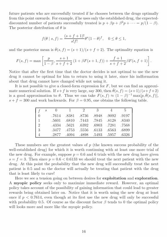
It is not possible to give a closed-form expression for F , but we can find an approxi-mate numerical solution. If s+f is very large, say 300, then θ(s, f) = (s+1)/(s+f+2)is a good approximation to θ. Thus we can take F (s, f) ≈ (1 − β)−1 max[p, θ(s, f)],s+ f = 300 and work backwards. For β = 0.95, one obtains the following table.

s 0 1 2 3 4 5f0 .7614 .8381 .8736 .8948 .9092 .91971 .5601 .6810 .7443 .7845 .8128 .83402 .4334 .5621 .6392 .6903 .7281 .75683 .3477 .4753 .5556 .6133 .6563 .68994 .2877 .4094 .4898 .5493 .5957 .6326

These numbers are the greatest values of p (the known success probability of thewell-established drug) for which it is worth continuing with at least one more trial ofthe new drug. For example, suppose p = 0.6 and 6 trials with the new drug have givens = f = 3. Then since p = 0.6 < 0.6133 we should treat the next patient with the newdrug. At this point the probability that the new drug will successfully treat the nextpatient is 0.5 and so the doctor will actually be treating that patient with the drugthat is least likely to cure!

Here we see a tension going on between desires for exploitation and exploration.A myopic policy seeks only to maximize immediate reward. However, an optimalpolicy takes account of the possibility of gaining information that could lead to greaterrewards being obtained later on. Notice that it is worth using the new drug at leastonce if p < 0.7614, even though at its first use the new drug will only be successfulwith probability 0.5. Of course as the discount factor β tends to 0 the optimal policywill looks more and more like the myopic policy.

16

5 Negative Programming

The special theory of minimizing nonnegative costs. We see that action that extremizes the

right hand side of the optimality equation is optimal. Stopping problems and OSLA rule.

5.1 Example: a partially observed MDP

Example 5.1. A hidden object moves between two location according to a Markovchain with probability transition matrix P = (pij). A search in location i costs ci,and if the object is there it is found with probability αi. The aim is to minimize theexpected cost of finding the object.

This is example of a partially observable Markov decision process (POMDP).The decision-maker cannot directly observe the underlying state, but he must maintaina probability distribution over the set of possible states, based on his observations, andthe underlying MDP. This distribution is updated by the usual Bayesian calculations.

Solution. Let xi be the probability that the object is in location i (where x1+x2 = 1).Value iteration of the dynamic programming equation is via

Fs(x1) = min

{

c1 + (1− α1x1)Fs−1

((1− α1)x1p11 + x2p21

1− α1x1

)

,

c2 + (1− α2x2)Fs−1

((1− α2)x2p21 + x1p11

1− α2x2

)}

.

The arguments of Fs−1(·) are the posterior probabilities that the object in location 1,given that we have search location 1 (or 2) and not found it.

Now F0(x1) = 0, F1(x1) = min{c1, c2}, F2(x) is the minimum of two linear functionsof x1. If Fs−1 is the minimum of some collection of linear functions of x1 it follows thatthe same can be said of Fs. Thus, by induction, Fs is a concave function of x1.

Since Fs → F in the N and F case, we can deduce that the infinite horizon returnfunction, F , is also a concave function. Notice that in the optimality equation for F(obtained by letting s → ∞ in the equation above), the left hand term within themin{·, ·} varies from c1 + F (p21) to c1 + (1 − α1)F (p11) as x1 goes from 0 to 1. Theright hand term varies from c2 + (1− α2)F (p21) to c2 + F (p11) as x1 goes from 0 to 1.

Consider the special case of α1 = 1 and c1 = c2 = c. Then the left hand term is thelinear function c + (1 − x1)F (p21). This means we have the picture below, where theblue and red curves corresponds to the left and right hand terms, and intersect exactlyonce since the red curve is concave.

Thus the optimal policy can be characterized as “search location 1 iff the probabilitythat the object is in location 1 exceeds a threshold x∗

1”.

17

0 1x1x∗

1

c+ F (p21)

c

c+ (1− α2)F (p21)

c+ F (p11)

The value of x∗1 depends on the parameters, αi and pij . It is believed the answer is

of this form for all values of the parameters, but this is still an unproved conjecture.

5.2 Stationary policies

A Markov policy is a policy that specifies the control at time t to be simply a functionof the state and time. In the proof of Theorem 4.2 we used ut = ft(xt) to specify thecontrol at time t. This is a convenient notation for a Markov policy, and we can writeπ = (f0, f1, . . . ) to denote such a policy. If in addition the policy does not depend ontime and is non-randomizing in its choice of action then it is said to be a deterministicstationary Markov policy, and we write π = (f, f, . . . ) = f∞.

For such a policy we might write

Ft(π, x) = c(x, f(x)) + E[Ft+1(π, x1) | xt = x, ut = f(x)]

or Ft+1 = L(f)Ft+1, where L(f) is the operator having action

L(f)φ(x) = c(x, f(x)) + E[φ(x1) | x0 = x, u0 = f(x)].

5.3 Characterization of the optimal policy

Negative programming is about maximizing non-positive rewards, r(x, u) ≤ 0, or min-imizing non-negative costs, c(x, u) ≥ 0. The following theorem gives a necessary andsufficient condition for a stationary policy to be optimal: namely, it must choose theoptimal u on the right hand side of the optimality equation. Note that in this theoremwe are requiring that the infimum over u is attained as a minimum over u (as wouldbe the case if we make the finite actions assumptions, F).

Theorem 5.2. Suppose D or N holds. Suppose π = f∞ is the stationary Markov policysuch that

f(x) = argminu

[c(x, u) + βE[F (x1) | x0 = x, u0 = u] .

Then F (π, x) = F (x), and π is optimal.

(i.e. u = f(x) is the value of u which minimizes the r.h.s. of the DP equation.)

18

Proof. The proof is really the same as the final part of proving Theorem 4.3. Bysubstituting the optimality equation into itself and using the fact that π specifies theminimizing control at each stage,

F (x) = Eπ

[s−1∑

t=0

βtc(xt, ut)

∣∣∣∣∣x0 = x

]

+ βsEπ [F (xs)|x0 = x] . (5.1)

In case N we can drop the final term on the right hand side of (5.1) (because it isnon-negative) and then let s → ∞; in case D we can let s → ∞ directly, observing thatthis term tends to zero. Either way, we have F (x) ≥ F (π, x).

A corollary is that if assumption F holds then an optimal policy exists. NeitherTheorem 5.2 or this corollary are true for positive programming (see Example 4.1).

5.4 Optimal stopping over a finite horizon

One way that the total-expected cost can be finite is if it is possible to enter a statefrom which no further costs are incurred. Suppose u has just two possible values: u = 0(stop), and u = 1 (continue). Suppose there is a termination state, say 0, that is enteredupon choosing the stopping action. Once this state is entered the system stays in thatstate and no further cost is incurred thereafter. We let c(x, 0) = k(x) (stopping cost)and c(x, 1) = c(x) (continuation cost). This defines a stopping problem.

Suppose that Fs(x) denotes the minimum total cost when we are constrained tostop within the next s steps. The dynamic programming equation is

Fs(x) = min{k(x), c(x) + E[Fs−1(x1) | x0 = x, u0 = 1]} , (5.2)

with F0(x) = k(x), c(0) = 0.Consider the set of states in which it is at least as good to stop now as to continue

one more step and then stop:

S = {x : k(x) ≤ c(x) + E[k(x1) | x0 = x, u0 = 1)]}.

Clearly, it cannot be optimal to stop if x 6∈ S, since in that case it would be strictlybetter to continue one more step and then stop. If S is closed then the followingtheorem gives us the form of the optimal policies for all finite-horizons.

Theorem 5.3. Suppose S is closed (so that once the state enters S it remains in S.)Then an optimal policy for all finite horizons is: stop if and only if x ∈ S.

Proof. The proof is by induction. If the horizon is s = 1, then obviously it is optimalto stop only if x ∈ S. Suppose the theorem is true for a horizon of s− 1. As above, ifx 6∈ S then it is better to continue for more one step and stop rather than stop in statex. If x ∈ S, then the fact that S is closed implies x1 ∈ S and so Fs−1(x1) = k(x1). Butthen (5.2) gives Fs(x) = k(x). So we should stop if s ∈ S.

The optimal policy is known as a one-step look-ahead rule (OSLA rule).

19

5.5 Example: optimal parking

A driver is looking for a parking space on the way to his destination. Each parkingspace is free with probability p independently of whether other parking spaces are freeor not. The driver cannot observe whether a parking space is free until he reaches it.If he parks s spaces from the destination, he incurs cost s, s = 0, 1, . . . . If he passesthe destination without having parked the cost is D. Show that an optimal policy isto park in the first free space that is no further than s∗ from the destination, where s∗

is the greatest integer s such that (Dp+ 1)qs ≥ 1.

Solution. When the driver is s spaces from the destination it only matters whetherthe space is available (x = 1) or full (x = 0). The optimality equation gives

Fs(0) = qFs−1(0) + pFs−1(1),

Fs(1) = min

{

s, (take available space)

qFs−1(0) + pFs−1(1), (ignore available space)

where F0(0) = D, F0(1) = 0.Now we solve the problem using the idea of a OSLA rule. It is better to stop now

(at a distance s from the destination) than to go on and take the first available spaceif s is in the stopping set

S = {s : s ≤ k(s− 1)}where k(s − 1) is the expected cost if we take the first available space that is s − 1 orcloser. Now

k(s) = ps+ qk(s− 1),

with k(0) = qD. The general solution is of the form k(s) = −q/p+ s + cqs. So aftersubstituting and using the boundary condition at s = 0, we have

k(s) = − q

p+ s+

(

D +1

p

)

qs+1, s = 0, 1, . . . .

SoS = {s : (Dp+ 1)qs ≥ 1}.

This set is closed (since s decreases) and so by Theorem 5.3 this stopping set describesthe optimal policy.

We might let D be the expected distance that that the driver must walk if he takesthe first available space at the destination or further down the road. In this case,D = 1 + qD, so D = 1/p and s∗ is the greatest integer such that 2qs ≥ 1.

20

6 Optimal Stopping Problems

More on stopping problems and their solution.

6.1 Bruss’s odds algorithm

A doctor, using a special treatment, codes 1 for a successful treatment, 0 otherwise. Hetreats a sequence of n patients and wants to minimize any suffering, while achievinga success with every patient for whom that is possible. Stopping on the last 1 wouldachieve this objective, so he wishes to maximize the probability of this.

Solution. Suppose Xk is the code of the kth patient. Assume X1, . . . , Xn are indepen-dent with pk = P (Xk = 1). Let qk = 1−pk and rk = pk/qk. Bruss’s odds algorithmsums the odds from the sth event to the last event (the nth)

Rs = rs + · · ·+ rn

and finds the greatest s, say s∗, for which Rs ≥ 1. We claim that by stopping thefirst time that code 1 occurs amongst patients {s∗, s∗+1, . . . , n}, the doctor maximizesprobability of stopping on the last patient who can be successfully treated.

To prove this claim we just check optimality of a OSLA-rule. The stopping set is

S = {i : qi+1 · · · qn > (pi+1qi+2qi+3 · · · qn) + (qi+1pi+2qi+3 · · · qn)+ · · ·+ (qi+1qi+2qi+3 · · · pn)}

= {i : 1 > ri+1 + ri+2 + · · ·+ rn}= {s∗, s∗ + 1, . . . , n}.

Clearly the stopping set is closed, so the OSLA-rule is optimal. The probability ofstopping on the last 1 is (qs∗ · · · qn)(rs∗ + · · ·+ rn) and (by solving a little optimizationproblem) this is always ≥ 1/e = 0.368, provided R1 ≥ 1.

We can use the odds algorithm to re-solve the secretary problem. Code 1 when acandidate is better than all who have been seen previously. Our aim is to stop on thelast candidate coded 1. We proved previously that X1, . . . , Xh are independent andP (Xt = 1) = 1/t. So ri = (1/t)/(1− 1/t) = 1/(t− 1). The algorithm tells us to ignorethe first s∗ − 1 candidates and the hire the first who is better than all we have seenpreviously, where s∗ is the greatest integer s for which

1

s− 1+

1

s+ · · ·+ 1

h− 1≥ 1

(

≡ the least s for which1

s+ · · ·+ 1

h− 1≤ 1

)

.

We can also solve a ‘groups’ version of the secretary problem. Suppose we seeh groups of candidates, of sizes n1, . . . , nh. We wish to stop with the group thatcontains the best of all the candidates. Then p1 = 1, p2 = n2/(n1 + n2), . . . , ph =nh/(n1 + · · · + nh). The odds algorithm tells us to stop if group i contains the bestcandidate so far and i ≥ s∗, where s∗ is the greatest integer s such that

ns∑s−1

i=1 ni

+ns+1∑s

i=1 ni+ · · ·+ nh

∑h−1i=1 ni

≥ 1.

21

6.2 Example: Stopping a random walk

Suppose that xt follows a random walk on {0, . . . , N}. At any time t we may stop thewalk and take a positive reward r(xt). In states 0 and N we must stop. The aim is tomaximize Er(xT ).

Solution. The dynamic programming equation is

F (0) = r(0), F (N) = r(N)

F (x) = max{r(x), 1

2F (x − 1) + 12F (x+ 1)

}, 0 < x < N.

We see that

(i) F (x) ≥ 12F (x− 1) + 1

2F (x+ 1), so F (x) is concave.

(ii) Also F (x) ≥ r(x).

We say F is a concave majorant of r.

In fact, F can be characterized as the smallest concave majorant of r. For supposethat G is any other concave majorant of r. Starting with F0 = 0, we have G ≥ F0. Sowe can prove by induction that

Fs(x) = max{r(x), 1

2Fs−1(x− 1) + 12Fs−1(x− 1)

}

≤ max{r(x), 1

2G(x− 1) + 12G(x + 1)

}

≤ max {r(x), G(x)}≤ G(x).

Theorem 4.3 tells us that Fs(x) → F (x) as s → ∞. Hence F ≤ G.A OSLA rule is not optimal here. The optimal rule is to stop iff F (x) = r(x).

6.3 Optimal stopping over the infinite horizon

Consider now a general stopping problem over the infinite-horizon with k(x), c(x) aspreviously, and with the aim of minimizing total expected cost. Let Fs(x) be the infimalcost given that we are required to stop by the sth step. Let F (x) be the infimal costwhen all that is required is that we stop eventually. Since less cost can be incurred ifwe are allowed more time in which to stop, we have

Fs(x) ≥ Fs+1(x) ≥ F (x).

Thus by monotone convergence Fs(x) tends to a limit, say F∞(x), and F∞(x) ≥ F (x).

Example 6.1. Consider the problem of stopping a symmetric random walk on theintegers, where c(x) = 0, k(x) = exp(−x). The policy of stopping immediately, say π,has F (π, x) = exp(−x), and since e−x is a convex function this satisfies the infinite-horizon optimality equation,

F (x) = min{exp(−x), (1/2)F (x− 1) + (1/2)F (x+ 1)}.

22

However, π is not optimal. The random walk is recurrent, so we may wait until reachingas large an integer as we like before stopping; hence F (x) = 0. Thus we see two things:

(i) It is possible that F∞ > F . This is because Fs(x) = e−x, but F (x) = 0.

(ii) Theorem 4.2 is not true for negative programming. Policy π has F (π, x) = e−x

and this satisfies the optimality equation. Yet π is not optimal.

Remark. In Theorem 4.3 we had F∞ = F , but for that theorem we assumed F0(x) =k(x) = 0 and Fs(x) was the infimal cost possible over s steps, and thus Fs ≤ Fs+1 (inthe N case). However, Example 6.1 k(x) > 0 and Fs(x) is the infimal cost amongst theset of policies that are required to stop within s steps. Now Fs(x) ≥ Fs+1(x).

The following lemma gives conditions under which the infimal finite-horizon costdoes converge to the infimal infinite-horizon cost.

Lemma 6.2. Suppose all costs are bounded as follows.

(a) K = supx

k(x) < ∞ (b) C = infxc(x) > 0. (6.1)

Then Fs(x) → F (x) as s → ∞.

Proof. Suppose π is an optimal policy for the infinite horizon problem and stops at therandom time τ . It has expected cost of at least (s + 1)CP (τ > s). However, since itwould be possible to stop at time 0 the cost is also no more than K, so

(s+ 1)CP (τ > s) ≤ F (x) ≤ K.

In the s-horizon problem we could follow π, but stop at time s if τ > s. This implies

F (x) ≤ Fs(x) ≤ F (x) +KP (τ > s) ≤ F (x) +K2

(s+ 1)C.

By letting s → ∞, we have F∞(x) = F (x).

Note that the problem posed here is identical to one in which we pay K at the startand receive a terminal reward r(x) = K − k(x).

Theorem 6.3. Suppose S is closed and (6.1) holds. Then an optimal policy for theinfinite horizon is: stop if and only if x ∈ S.

Proof. By Theorem 5.3 we have for all finite s,

Fs(x)= k(x) x ∈ S,< k(x) x 6∈ S.

Lemma 6.2 gives F (x) = F∞(x).

23

6.4 Sequential Probability Ratio Test

A statistician wishes to decide between two hypotheses, H0 : f = f0 and H1 : f = f1on the basis of i.i.d. observations drawn from a distribution with density f . Ex ante hebelieves the probability that Hi is true is pi (where p0 + p1 = 1). Suppose that he hasthe sample x = (x1, . . . , xn). The posterior probabilities are in the likelihood ratio

ℓn(x) =f1(x1) · · · f1(xn)

f0(x1) · · · f0(xn)

p1p0

.

Suppose it costs γ to make an observation. Stopping and declaring Hi true results ina cost ci if wrong. This leads to the optimality equation for minimizing expected cost

F (ℓ) = min

{

c0ℓ

1 + ℓ, c1

1

1 + ℓ,

γ +ℓ

1 + ℓ

∫

F (ℓf1(y)/f0(y))f1(y)dy +1

1 + ℓ

∫

F (ℓf1(y)/f0(y))f0(y)dy

}

Taking H(ℓ) = (1 + ℓ)F (ℓ), the optimality equation can be rewritten as

H(ℓ) = min

{

c0ℓ, c1, (1 + ℓ)γ +

∫

H(ℓf1(y)/f0(y))f0(y)dy

}

.

This is a similar problem to the one we solved about searching for a hidden object. Thestate is ℓn. We can stop (in two ways) or continue by paying for another observation,in which case the state makes a random jump to ℓn+1 = ℓnf1(x)/f0(x), where x is anobservation from f0. We can show that H(·) is concave in ℓ, and that therefore theoptimal policy can be described by two numbers, a∗0 ≤ a∗1: If ℓn ≤ a∗0, stop and declareH0 true; If ℓn ≥ a∗1, stop and declare H1 true; otherwise take another observation.

6.5 Bandit processes

A bandit process is a special type of MDP in which there are just two possible actions:u = 0 (freeze) or u = 1 (continue). The control u = 0 produces no reward and the statedoes not change (hence the term ‘freeze’). Under u = 1 we obtain a reward r(xt) andthe state changes, to xt+1, according to the Markov dynamics P (xt+1 | xt, ut = 1).

A simple family of alternative bandit processes (SFABP) is a collection of nsuch bandit processes. At each time t = 0, 1, . . . we must select exactly one bandit toreceive the continuation action, while all others are frozen.

This provide a very rich modelling framework. With it we can model questions like:

• Which of n drugs should we give to the next patient?

• Which of n jobs should we work on next?

• When of n oil fields should we explore next?

24

7 Bandit Processes and the Gittins Index

The multi-armed bandit problem. Gittins index theorem.

7.1 Multi-armed bandit problem

A multi-armed bandit is a slot-machine with multiple arms. The arms differ in thedistributions of rewards that they pay out when pulled. An important special case iswhen arm i is a so-called Bernoulli bandit, with parameter pi. We have already metthis as the drug-testing model in §4.5. Such an arm pays £1 with probability pi, and£0 with probability 1− pi; this happens independently each time the arm is pulled. Ifthere are n such arms, and a gambler knows the true values of p1, . . . , pn, then obviouslyhe maximizes his expected reward by always pulling the arm of maximum pi. However,if he does not know the pi, then he must choose each successive arm on the basis of theinformation he has obtained by playing, updated in a Bayesian manner on the basis ofobserving the rewards he has obtained on previous pulls. The aim in the multi-armedbandit problem (MABP) is to maximize the expected total discounted reward.

More generally, we consider a problem of controlling the evolution of n indepen-dent reward-producing Markov processes decision processes. The action space of eachprocess contains just two controls, which cause the process to be either ‘continued’ or‘frozen’. At each instant (in discrete time) exactly one of these so-called bandit pro-cesses is continued (and reward from it obtained), while all the other bandit processesare frozen. The continued process can change state; but frozen processes do not changestate. Reward is accrued only from the bandit process that is continued. This createswhat is termed a simple family of alternative bandit processes (SFABP). Theword ‘simple’ means that all the n bandit processes are available at all times.

Let x(t) = (x1(t), . . . , xn(t)) be the states of the n bandits. Let it denote the banditprocess that is continued at time t under some policy π. In the language of Markovdecision problems, we wish to find the value function:

F (x) = supπ

E

[∞∑

t=0

rit(xit(t))βt

∣∣∣∣∣x(0) = x

]

,

where the supremum is taken over all policies π that are realizable (or non-anticipatory),in the sense that it depends only on the problem data and x(t), not on any informationwhich only becomes known only after time t.

Setup in this way, we have an infinite-horizon discounted-reward Markov decisionproblem. It therefore has a deterministic stationary Markov optimal policy. Its dynamicprogramming is

F (x) = maxi:i∈{1,...,n}

ri(x) + β

∑

y∈Ei

Pi(xi, y)F (x1, . . . , xi−1, y, xi+1, . . . , xn)

. (7.1)

25

7.2 The two-armed bandit

Consider first a problem with one arm B1 which always pays λ, and a second arm ofgeneral type. The optimality equation, when B2 is in its state x, is

F (x) = max

{

λ

1− β, r(x) + β

∑

y

P (x, y)F (y)

}

= max

{

λ

1− β, sup

τ>0E

[τ−1∑

t=0

βtr(x(t)) + βτ λ

1− β

∣∣∣ x(0) = x

]}

.

The left hand choice within max{·, ·} corresponds to continuing B1. The right handchoice corresponds to continuing B2 for at least one step and then switching to B1 asome later step, τ . Notice that once we switch to B1 we will never wish switch back toB2 because things remain the same as when we first switched away from B2.

We are to choose the stopping time τ so as to optimally switch from continuingB2 to continuing B1. Because the two terms within the max{·, ·} are both increasingin λ, and are linear and convex, respectively, there is a unique λ, say λ∗, for which theyare equal.

λ∗ = sup

{

λ :λ

1− β≤ sup

τ>0E

[τ−1∑

t=0

βtr(x(t)) + βτ λ

1− β

∣∣∣ x(0) = x

]}

. (7.2)

Of course this λ depends on x(0). We denote its value as G(x). After a little algebra

G(x) = supτ>0

E[∑τ−1

t=0 βtr(x(t)∣∣∣ x(0) = x

]

E[∑τ−1

t=0 βt∣∣∣ x(0) = x

] . (7.3)

G(x) is called the Gittins index (of state x), named after its originator, John Gittins.The definition above is by a calibration, the idea being that we find a B1 paying aconstant reward λ, such that we are indifferent as to which bandit to continue next.

In can be easily shown that τ = min{t : Gi(xi(t)) ≤ Gi(xi(0)), τ > 0}, that is, τ isthe first time B2 is in a state where its Gittins index is no greater than it was initially.

In (7.3) we see that the Gittins index is the maximal possible quotient of ‘expectedtotal discounted reward over τ steps’, divided by ‘expected total discounted time overτ steps’, where τ is at least 1 step. The Gittins index can be computed for all statesof Bi as a function only of the data ri(·) and Pi( · , · ). That is, it can be computedwithout knowing anything about the other bandit processes.

7.3 Gittins index theorem

Remarkably, the problem posed by a SFABP (or a MABP) can be solved by using theseGittins indices.

26

Theorem 7.1 (Gittins Index Theorem). The problem posed by a SFABP, as setupabove, is solved by always continuing the process having the greatest Gittins index.

The Index Theorem is due to Gittins and Jones, who had obtained it by 1970, andpresented it in 1972. The solution of the MABP impressed many experts as surpris-ing and beautiful. Peter Whittle describes a colleague of high repute, asking anothercolleague ‘What would you say if you were told that the multi-armed bandit problemhad been solved?’ The reply was ‘Sir, the multi-armed bandit problem is not of such anature that it can be solved ’.

Single machine scheduling. Recall the example in §3.2 in which n jobs are to beprocessed successively on one machine. Job i has a known processing times ti, assumedto be a positive integer. On completion of job i a positive reward ri is obtained. Weused an interchange argument to show that the discounted sum of rewards is maximizedby processing jobs in decreasing order of the index riβ

t1/(1− βt1).Now we do this using Gittins index. The optimal stopping time on the right hand

side of (7.3) is τ = ti, the numerator is riβti and the denominator is 1+β+· · ·+βti−1 =

(1− βti)/(1− β). Thus, Gi = riβti(1− β)/(1− βti). Note that Gi → ri/ti as β → 1.

7.4 Playing golf with many balls

There have been many proofs of the index theorem, all of which are useful in developinginsight. The following proof is perhaps the simplest (due to Weber (1992)). It is funto explain it in a special context (invented by Dimitri, Tetali and Winkler, 2003).

A golfer is playing with n balls. They are at positions x1, . . . , xn. If he plays balli it will next land at location y with probability P (xi, y). He wishes to minimize theexpected number of shots taken to get one ball in the hole (location 0).

To represent this as a SFABP we set rewards and costs all 0, except that a rewardR is obtained by continuing a bandit that is in state 0. So if some bandit (ball) reachesstate 0, say with the golfer’s tth shot, he will continue to play it there, obtaining reward(βt + βt+1 + · · · )R. Suppose the golfer pays a ‘green fee’ of R/(1 − β). Then he willbe trying to maximize

− R

1− β+ (βt + βt+1 + · · · )R = −(1 + β + · · ·+ βt−1)R

which tends to −tR as β → 1, so he’ll want to minimize the expected number of shotstaken to sink a ball. We claim this problem can be solved by a (Gittins) index policy.

Proof. Suppose the golfer is playing with just one ball, which is in location xi. Thegolfer faces a cost of 1 for each shot he takes until the ball is sunk. So to motivate himto play on, we offer him a prize g(xi) which he receives if he plays at least one moreshot and eventually sinks the ball. He is allowed to quit subsequently if the ball landsin a bad place and the offered prize is no longer sufficiently motivating. But if this everhappens, we will increase the offered prize, so that it again becomes just advantageous

27

for him to keep playing. This defines an nondecreasing sequence of offered prizes forball i. Notice that it is defined independently of the other balls.

Now he plays with n balls. For each of them we define an offered prize, as above.It is a function of its location, just as if he were playing only with that ball.

The key idea is that with these offered prizes the golfer can keep playing until a ballis sunk, and he will just break even. He is guaranteed to collect the least possible prizewhen a ball is finally sunk if he follows the policy of always playing the ball for whichthe least prize is on offer. But the prizes were invented to make the game is ‘just fair’,and so this policy must also minimize the expected number of shots required to sink aball in the hole. The prize g(xi) is of course the Gittins index for location xi.

7.5 Example: Weitzman’s problem

‘Pandora’ has n boxes, each of which contains an unknown prize. Ex ante the prize inbox i has a value with probability distribution function Fi. She can learn the value ofthe prize by opening box i, which costs her ci to do. At any stage she may stop andtake as her reward the maximum of the prizes she has found. She wishes to maximizethe expected value of the prize she takes, minus the costs of opening boxes.

Solution. This problem can be modelled as a SFABP. Box i is associated with a banditprocess Bi, which starts in state 0. The first time it is ‘continued’ there is a cost ci,and the state becomes xi, chosen by the distribution Fi. At all subsequent times thatit is continued the reward is r(xi) = (1 − β)xi, and the state remains xi. We wish tomaximize the expected value of

−τ∑

t=1

βt−1cit +max{r(xi1 ), . . . , r(xiτ )}∞∑

t=τ

βt

where we open boxes i1, . . . , iτ and then take the best prize thereafter. In the limit asβ → 1 this objective corresponds to that of Weitzman’s problem, namely,

−τ∑

t=1

cit +max{xi1 , . . . , xiτ }

and so we can find the solution using the Gittins index theorem.The Gittins index of an opened box is r(xi). The index of an unopened box i is the

solution toGi

1− β= −ci +

β

1− βEmax{r(xi), Gi}

or, by setting gi = G/(1 − β), and letting β → 1, we get an index that is the solutionof gi = −ci + Emax{xi, gi}.

For example, if Fi is a two point distribution with xi = 0 or xi = ri, with probabil-ities 1− pi and pi, then gi = −ci + (1− pi)gi + piri =⇒ gi = ri − ci/pi.

Pandora’s optimal strategy is thus: Open boxes in decreasing order of gi until firstreaching a point that a revealed prize is greater than all gi of unopened boxes.

28

7.6 *Calculation of the Gittins index*

How can we compute the Gittins index value for each possible state of a bandit processBi? The input is the data of ri(·) and Pi(·, ·). If the state space of Bi is finite, sayEi = {1, . . . , ki}, then the Gittins indices can be computed in an iterative fashion. Firstwe find the state of greatest index, say 1 such that 1 = argmaxj ri(j). Having foundthis state we can next find the state of second-greatest index. If this is state j, thenGi(j) is computed in (7.3) by taking τ to be the first time that the state is not 1. Thismeans that the second-best state is the state j which maximizes

E[ri(j) + βri(1) + · · ·+ βτ−1ri(1)]

E[1 + β + · · ·+ βτ−1],

where τ is the time at which, having started at xi(0) = j, we have xi(τ) 6= 1. Onecan continue in this manner, successively finding states and their Gittins indices, indecreasing order of their indices. If Bi moves on a finite state space of size ki then itsGittins indices (one for each of the ki states) can be computed in time O(k3i ).

If the state space of a bandit process is infinite, as in the case of the Bernoullibandit, there may be no finite calculation by which to determine the Gittins indices forall states. In this circumstance, we can approximate the Gittins index using somethinglike the value iteration algorithm. Essentially, one solves a problem of maximizing righthand side of (7.3), subject to τ ≤ N , where N is large.

7.7 *Forward induction policies*

If we put τ = 1 on the right hand side of (7.3) then it evaluates to Eri(xi(t)). Ifwe use this as an index for choosing between projects, we have a myopic policy orone-step-look-ahead policy. The Gittins index policy generalizes the idea of a one-step-look-ahead policy, since it looks-ahead by some optimal time τ , so as to maximize,on the right hand side of (7.3), a measure of the rate at which reward can be accrued.This defines a so-called forward induction policy.

7.8 *Proof of the Gittins index theorem*

The proof in the §7.4 has all the key ideas. For completeness we give a fuller proof ofthe Gittins index theorem.

Proof of Theorem 7.1. We start by considering a problem in which only bandit processBi is available. Let us define the fair charge, γi(xi), as the maximum amount that agambler would be willing to pay per step in order to be permitted to continue Bi for atleast one more step, and being free to stop continuing it whenever he likes thereafter.This is

γi(xi) = sup

{

λ : 0 ≤ supτ>0

E

[τ−1∑

t=0

βt(

ri(xi(t))− λ) ∣∣∣xi(0) = xi

]}

. (7.4)

29

Notice that (7.2) and (7.4) are equivalent definitions and so γi(xi) = Gi(xi). Noticealso that the time τ will be the first time that Gi(xi(τ)) < Gi(xi(0)).

We next define the prevailing charge for Bi at time t as gi(t) = mins≤t γi(xi(s)).So gi(t) actually depends on xi(0), . . . , xi(t) (which we omit from its argument forconvenience). Note that gi(t) is a nonincreasing function of t and its value dependsonly on the states through which bandit i evolves. The proof of the Index Theorem iscompleted by verifying the following facts, each of which is almost obvious.

(i) Suppose that in the problem with n available bandit processes, B1, . . . , Bn, theagent not only collects rewards, but also pays the prevailing charge of whateverbandit that he chooses to continue at each step. Then he cannot do better thanjust break even (i.e. expected value of rewards minus prevailing charges is 0).

This is because he could only make a strictly positive profit (in expected value) ifthis were to happens for at least one bandit. Yet the prevailing charge has beendefined in such a way that he can only just break even.

(ii) If he always continues the bandit of greatest prevailing charge then he will inter-leave the n nonincreasing sequences of prevailing charges into a single nonincreas-ing sequence of prevailing charges and so maximize their discounted sum.

(iii) Using this strategy he also just breaks even; so this strategy, (of always continuingthe bandit with the greatest gi(xi)), must also maximize the expected discountedsum of the rewards can be obtained from this SFABP.

30

8 Average-cost Programming

The average-cost optimality equation. Policy improvement algorithm.

8.1 Average-cost optimality equation

Suppose that for a stationary Markov policy π, the following limit exists:

λ(π, x) = limt→∞

1

tEπ

[t−1∑

τ=0

c(xτ , uτ )

∣∣∣∣∣x0 = x

]

.

We might expect there to be a well-defined notion of an optimal average-cost, λ(x) =infπ λ(π, x), and that under appropriate assumptions, λ(x) = λ should not depend onx. Moreover, a reasonable guess is that

Fs(x) = sλ+ φ(x) + ǫ(s, x),

where ǫ(s, x) → 0 as s → ∞. Here φ(x) + ǫ(s, x) reflects a transient due to the initialstate. Suppose that the state space and action space are finite. From the optimalityequation for the finite horizon problem we have

Fs(x) = minu

{c(x, u) + E[Fs−1(x1) | x0 = x, u0 = u]}. (8.1)

So by substituting Fs(x) ∼ sλ+ φ(x) into (8.1), we obtain

sλ+ φ(x) ∼ minu

{c(x, u) + E[(s− 1)λ+ φ(x1) | x0 = x, u0 = u]}

which suggests that the average-cost optimality equation should be:

λ+ φ(x) = minu

{c(x, u) + E[φ(x1) | x0 = x, u0 = u]}. (8.2)

Theorem 8.1. Suppose there exists a constant λ and bounded function φ satisfying(8.2). Let π be the policy which in each state x chooses u to minimize the right handside. Then λ is the minimal average-cost and π is the optimal stationary policy.

Proof. Suppose u is chosen by some policy π′. By repeated substitution of (8.2) intoitself we have

φ(x) ≤ −tλ+ Eπ′

[t−1∑

τ=0

c(xτ , uτ)

∣∣∣∣∣x0 = x

]

+ Eπ′ [φ(xt) | x0 = x].

with equality if π′ = π. Divide this by t and let t → ∞. Boundedness of φ ensures that(1/t)Eπ′ [φ(xt) | x0 = x] → 0. So we obtain

0 ≤ −λ+ limt→∞

1

tEπ′

[t−1∑

τ=0

c(xτ , uτ )

∣∣∣∣∣x0 = x

]

,

with equality if π′ = π.

31

So an average-cost optimal policy can be found by looking for a bounded solutionto (8.2). Notice that if φ is a solution of (8.2) then so is φ+(a constant), because the (aconstant) will cancel from both sides of (8.2). Thus φ is undetermined up to an additiveconstant. In searching for a solution to (8.2) we can therefore pick any state, say x,and arbitrarily take φ(x) = 0. The function φ is called the relative value function.

8.2 Example: admission control at a queue

Each day a consultant is presented with the opportunity to take on a new job. Thejobs are independently distributed over n possible types and on a given day the offeredtype is i with probability ai, i = 1, . . . , n. Jobs of type i pay Ri upon completion.Once he has accepted a job he may accept no other job until that job is complete. Theprobability that a job of type i takes k days is (1− pi)

k−1pi, k = 1, 2, . . . . Which jobsshould the consultant accept?

Solution. Let 0 and i denote the states in which he is free to accept a job, and inwhich he is engaged upon a job of type i, respectively. Then (8.2) is

λ+ φ(0) =

n∑

i=1

aimax[φ(0), φ(i)],

λ+ φ(i) = (1− pi)φ(i) + pi[Ri + φ(0)], i = 1, . . . , n.

Taking φ(0) = 0, these have solution φ(i) = Ri − λ/pi, and hence

λ =

n∑

i=1

aimax[0, Ri − λ/pi].

The left hand side is increasing in λ and the right hand side is decreasing λ. Hencethere is a root, say λ∗, and this is the maximal average-reward. The optimal policytakes the form: accept only jobs for which piRi ≥ λ∗.

8.3 Value iteration bounds

Value iteration in the average-cost case is based upon the idea that Fs(x) − Fs−1(x)approximates the minimal average-cost for large s. For the rest of this lecture wesuppose the state space is finite.

Theorem 8.2. Define

ms = minx

{Fs(x) − Fs−1(x)}, Ms = maxx

{Fs(x) − Fs−1(x)}. (8.3)

Then ms ≤ λ ≤ Ms, where λ is the minimal average-cost.

32

Proof. Suppose π = f∞ is the average-cost optimal policy over the infinite horizon,taking u = f(x), with average-cost λ. Then

Fs−1(x) +ms ≤ Fs−1(x) + [Fs(x) − Fs−1(x)]

= Fs(x)

≤ c(x, f(x)) + E[Fs−1(x1) | x0 = x, u0 = f(x)].

We substitute this into itself t− 1 times to get

Fs−1(x) ≤ −mst+ Eπ

[t−1∑

τ=0

c(xτ , uτ)

∣∣∣∣∣x0 = x

]

+ Eπ[Fs−1(xt) | x0 = x].

Divide by t and let t → ∞ to get ms ≤ λ. A bound λs ≤ Ms is found similarly using

Fs−1(x) ≥ −Ms + c(x, u) + E[Fs−1(x1) | x0 = x, u0 = fs(x)].

≥ −Mst+ Eπs

[t−1∑

τ=0

c(xτ , uτ )

∣∣∣∣∣x0 = x

]

+ Eπs[Fs−1(xt) | x0 = x].

This justifies use of a value iteration algorithm in which we calculate Fs untilMs −ms ≤ ǫms. At that point the stationary policy f∞

s achieves an average-cost thatis within ǫ× 100% of optimal.

8.4 Policy improvement algorithm

In the average-cost case a policy improvement algorithm is be based on the follow-ing observations. Suppose that for a policy π = f∞, we have that λ, φ solve

λ+ φ(x) = c(x, f(x0)) + E[φ(x1) | x0 = x, u0 = f(x0)],

and there exists a policy π1 = f∞1 such that

λ+ φ(x) ≥ c(x, f1(x0)) + E[φ(x1) | x0 = x, u0 = f1(x0)], (8.4)

for all x, and with strict inequality for some x (and thus f1 6= f). Then following thelines of proof in Theorems 8.1 and 8.2 (repeatedly substituting (8.4) into itself),

λ ≥ limt→∞

1

tEπ1

[t−1∑

τ=0

c(xτ , uτ)

∣∣∣∣∣x0 = x

]

. (8.5)

So π1 is at least as good as π. If there is no π1 then π satisfies (8.2) and so π is optimal.This justifies the following policy improvement algorithm

33

(0) Choose an arbitrary stationary policy π0. Set s = 1.

(1) For stationary policy πs−1 = f∞s−1 determine φ, λ to solve

λ+ φ(x) = c(x, fs−1(x)) + E[φ(x1) | x0 = x, u0 = fs−1(x)].

This gives a set of linear equations, and so is intrinsically easier to solve than (8.2).The average-cost of πs−1 is λ.

(2) Now determine the policy πs = f∞s from

fs(x) = argminu

{c(x, u) + E[φ(x1) | x0 = x, u0 = u]},

taking fs(x) = fs−1(x) whenever this is possible. If πs = πs−1 then we have a solutionto (8.2) and so πs−1 is optimal. Otherwise πs is a new policy. By the calculation in(8.5) this has an average-cost no more than λ, so πs is at least as good as πs−1, Wenow return to step (1) with s := s+ 1.

If both the action and state spaces are finite then there are only a finite numberof possible stationary policies and so the policy improvement algorithm must find anoptimal stationary policy in finitely many iterations. By contrast, the value iterationalgorithm only obtains increasingly accurate approximations of λ∗.

Example 8.3. Consider again the example of §8.2. Let us start with a policy π0 whichaccept only jobs of type 1. The average-cost of this policy can be found by solving

λ+ φ(0) = a1φ(1) +

n∑

i=2

aiφ(0),

λ+ φ(i) = (1− pi)φ(i) + pi[Ri + φ(0)], i = 1, . . . , n.

The solution is λ = a1p1R1/(a1 + p1), φ(0) = 0, φ(1) = p1R1/(a1 + p1), and φ(i) =Ri − λ/pi, i ≥ 2. The first use of step (1) of the policy improvement algorithm willcreate a new policy π1, which improves on π0, by accepting jobs for which φ(i) =max{φ(0), φ(i)}, i.e. for which φ(i) = Ri − λ/pi > 0 = φ(0).

If there are no such i then π0 is optimal. So we may conclude that π0 is optimal ifand only if piRi ≤ a1p1R1/(a1 + p1) for all i ≥ 2.

Policy improvement in the discounted-cost case.

In the case of strict discounting the policy improvement algorithm is similar:

(0) Choose an arbitrary stationary policy π0. Set s = 1.

(1) For stationary policy πs−1 = f∞s−1 determine G to solve

G(x) = c(x, fs−1(x)) + βE[G(x1) | x0 = x, u0 = fs−1(x)].

(2) Now determine the policy πs = f∞s from

fs(x) = argminu

{c(x, u) + βE[G(x1) | x0 = x, u0 = u]},

taking fs(x) = fs−1(x) whenever this is possible. Stop if fs = fs−1. Otherwise returnto step (1) with s := s+ 1.

34

9 Continuous-time Markov Decision Processes

Control problems in a continuous-time stochastic setting. Markov jump processes when the

state space is discrete. Uniformization.

9.1 Stochastic scheduling on parallel machines

A collection of n jobs is to be processed on a single machine. They have processingtimes X1, . . . , Xn, which are ex ante distributed as independent exponential randomvariables, Xi ∼ E(λi) and EXi = 1/λi, where λ1, . . . , λn are known.

If jobs are processed in order 1, 2, . . . , n, they finished in expected time 1/λ1+ · · ·+1/λn. So the order of processing does not matter.

But now suppose there are m (2 ≤ m < n) identical machines working in parallel.Let Ci be the completion time of job i.

• maxi Ci is called the makespan (the time when all jobs are complete).

• ∑i Ci is called the flow time (sum of completion times).

Suppose we wish to minimize the expected makespan. We can find the optimalorder of processing by stochastic dynamic programming. But now we are in continuoustime, t ≥ 0. So we need the important facts:

(i) min(Xi, Xj) ∼ E(λi + λj); (ii) P (Xi < Xj | min(Xi, Xj) = t) = λi/(λi + λj).

Suppose m = 2. The optimality equations are

F ({i}) = 1

λi

F ({i, j}) = 1

λi + λj[1 + λiF ({j}) + λjF ({i})]

F (S) = mini,j∈S

1

λi + λj[1 + λiF (Si) + λjF (Sj)],

where S is a set of uncompleted jobs, and we use the abbreviated notation Si = S \{i}.It is helpful to rewrite the optimality equation. Let Λ =

∑

i λi. Then

F (S) = mini,j∈S

1

Λ

1 + λiF (Si) + λjF (Sj) +∑

k 6=i,j

λkF (S)

= minui∈[0,1],i∈S,∑

iui≤2

1

Λ

[

1 + ΛF (S) +∑

i

uiλi(F (Si)− F (S))

]

This is helpful, because in all equations there is now the same divisor, Λ. An eventoccurs after a time that is exponentially distributed with parameter Λ, but with proba-bility λk/Λ this is a ‘dummy event’ if k 6= i, j. This trick is known as uniformization.Having set this up we might also then say let Λ = 1.

35

We see that it is optimal to start by processing the two jobs in S for which δi(S) :=λi(F (Si)− F (S)) is least.

The policy of always processing the m jobs of smallest [largest] λi is called theLowest [Highest] Hazard Rate first policy, and denoted LHR [HHR] .

Theorem 9.1.(a) Expected makespan is minimized by LHR.

(b) Expected flow time is minimized by HHR.

(c) E[C(n−m+1)] (expected time there is first an idle machine) is minimized by LHR.

Proof. (*starred*) We prove only (a), and for ease assume m = 2 and λ1 < · · · < λn.We would like to prove that for all i, j ∈ S ⊆ {1, . . . , n},

i < j ⇐⇒ δi(S) < δj(S) (except possibly if both i and j

are the jobs that would be processed by the optimal policy).(9.1)

Truth of (9.1) would imply that jobs should be started in the order 1, 2, . . . , n.Stochastic sequential assignment problem with arrivalsLet π be LLR. Take an induction hypothesis that (9.1) is true and that F (S) =

F (π, S) when S is a strict subset of {1, . . . , n}. Now consider S = {1, . . . , n}. Weexamine F (π, S), and δi(π, S), under π. Let S

k denote S \ {k}. For i ≥ 3,

F (π, S) =1

λ1 + λ2[1 + λ1F (S1) + λ2F (S2)]

F (π, Si) =1

λ1 + λ2[1 + λ1F (S1i) + λ2F (S2i)]

=⇒ δi(π, S) =1

λ1 + λ2[λ1δi(S

1) + λ2δi(S2)], i ≥ 3. (9.2)

If for some 3 ≤ i < j we were to have δi(π, S) > δj(π, S) then this would require thateither δi(S

1) > δj(S1) or δi(S

2) > δj(S2). But our induction hypothesis for (9.1) rules

these out.Similarly, we can compute δ1(π, S).

F (π, S) =1

λ1 + λ2 + λ3[1 + λ1F (S1) + λ2F (S2) + λ3F (π, S)]

F (π, S1) =1

λ1 + λ2 + λ3[1 + λ1F (S1) + λ2F (S12) + λ3F (S13)]

=⇒ δ1(π, S) =1

λ1 + λ2 + λ3[λ2δ1(S

2) + λ3δ1(π, S) + λ1δ3(S1)]

=1

λ1 + λ2[λ1δ3(S

1) + λ2δ1(S2)]. (9.3)

By comparing (9.2) and (9.3) we see that we could only have δi(S) < δ1(S) for i ≥ 3 ifat least one of δi(S

1) < δ3(S1) or δi(S

2) < δ1(S2) is true. These are ruled out by our

induction hypothesis. Similarly, we cannot have δi(S) < δ2(S) for i ≥ 3.

36

This completes a step of a step of an inductive proof by showing that (9.1) is truefor S, and that F (S) = F (π, S). We only need to check the base of the induction. Thisis provided by the simple calculation

δ1({1, 2}) = λ1(F ({2})− F ({1, 2})) = λ1

[1

λ2− 1

λ1 + λ2

(

1 +λ1

λ2+

λ2

λ1

)]

= − λ2

λ1 + λ2≤ δ2({1, 2}).

The proof of (b) is very similar, except that the inequality in (9.1) should be reversed.The base of the induction comes from δ1({1, 2}) = −1.

The proof of (c) is also similar. The base of the induction is provided by δ1({1, 2}) =λ1(0 − 1/(λ1 + λ2)). Since we are seeking to maximize EC(n−m+1) we should processjobs for which δi is greatest, i.e., least λi. The problem in (c) is known as the Lady’snylon stocking problem. We think of a lady (having m = 2 legs) who wears twostockings each day, which may fail, and she wishes to maximize the expected time untilshe has only one good stocking left to wear.

9.2 Controlled Markov jump processes

The above example illustrates the idea of a controlled Markov jump process. Itevolves in continuous time, and in a discrete state space. In general:

• The state is i. We choose some control, say u (u ∈ A(i), a set of availablecontrols).

• After a time that is exponentially distributed with parameter qi(u) =∑

j 6=i qij(u),(i.e. having mean 1/qi(u)), the state jumps.

• Until the jump occurs cost accrues at rate c(i, u).

• The jump is to state j (6= i) with probability qij(u)/qi(u).

The infinite-horizon optimality equation is

F (i) = minu∈A(i)

1

qi(u)

c(i, u) +∑

j

qij(u)F (j)

.

Suppose qi(u) ≤ B for all i, u and use the uniformization trick,

F (i) = minu∈A(i)

1

B

c(i, u) + (B − qi(u))F (i) +∑

j

qij(u)F (j)

.

We now have something that looks exactly like a discrete-time optimality equation

F (i) = minu∈A(i)

c(i, u) +

∑

j

pij(u)F (j)

37

where c(i, u) = c(i, u)/B, pij(u) = qij(u)/B, j 6= i, and Pii(u) = 1− qi(u)/B.This is great! It means we can use all the methods and theorems that we have

developed previously for solving discrete-time dynamic programming problems.We can also introduce discounting by imagining that there is an ‘exponential clock’

of rate α which takes the state to a place where no further cost or reward is obtained.This leads to an optimality equation of the form

F (i) = minu

c(i, u) + β

∑

j

pij(u)F (j)

,

where β = B/(B + α), c(i, u) = c(i, u)/(B + α), and pij(u) is as above.

9.3 Example: admission control at a queue

The number of customers waiting in a queue is 0, 1, . . . . There is a constant servicerate µ (meaning that the service times of customers are distributed E(µ), and we maycontrol the arrival rate u between 0 and a maximum value M . Let c(x, u) = ax− Ru.There is a holding cost a per unit time for each customer in the queue and receivinga reward R at the point that each new customer is admitted (and therefore incurringreward at rate Ru when the arrival rate is u). Suppose there is discounting at rate α.The problem is one of choosing 0 ≤ ut ≤ M to minimize

E

[∫ ∞

0

(axt −Rut)e−αtdt

]

.

Let us take B = α+M + µ, and without loss of generality assume B = 1.After uniformization the discounted-cost optimality equation will look like

F (0) = infu∈[0,M ]

{−Ru+ β[uF (1) + (M − u)F (j − 1)]}

F (x) = infu∈[0,M ]

{ax− Ru+ β[uF (x+ 1) + µF (x− 1) + (M − u)F (x)]}, x ≥ 1.

So we can see that the optimal control is bang-bang, taking u = 0 or u = M as thecoefficient of u, namely −R+ F (x+ 1)− F (x), is positive or negative. One can set upa value iteration form of this, i.e.

Fk+1(0) = infu∈[0,M ]

{−Ru+ β[uFk(1) + (M − u)Fk(j − 1)]}

Fk+1(x) = infu∈[0,M ]

{ax−Ru+ β[uFk(x+ 1) + µFk(x − 1) + (M − u)Fk(x)]}, x ≥ 1

and then prove by induction that Fk(x) is concave in x. This means that there existsa threshold rule such that the optimal policy will be of the form:

u =

{

0

Mas x

≥<

x∗.

38

Time-average cost optimality. The optimality equation is

φ(0) + γ = infu∈[0,M ]

[−Ru+ uφ(1) + (µ+M − u)φ(0)],

= infu∈[0,M ]

[u{−R+ φ(1)− φ(0)} + (µ+M)φ(0)],

φ(x) + γ = infu[ax−Ru+ uφ(x+ 1) + µφ(x− 1) + (M − u)φ(x)],

= infu∈[0,M ]

[ax+ u{−R+ φ(x + 1)− φ(x)} + µφ(x− 1) +Mφ(x)], x ≥ 1.

Thus u should be chosen to be 0 or M as −R+ φ(x+1)− φ(x) is positive or negative.Let us consider what happens under the policy that take u = M for all x. The

relative costs for this policy, say f , are given by

f(x) + γ = ax−Rλ+Mf(x+ 1) + µf(x− 1), x ≥ 1.

The solution to the homogeneous part of this recursion is of the form f(x) = d11x +

d2(µ/M)x. Assuming M < µ and we desire a solution for f that does not growexponentially, we take d2 = 0 and so the solution is effectively the solution to theinhomogeneous part, i.e.

f(x) =ax(x+ 1)

2(µ−M), γ =

aM

µ−M−MR,

Applying the idea of policy improvement, we conclude that a better policy is to takeu = 0 (i.e. don’t admit a customer) if −R+ f(x+ 1)− f(x) > 0, i.e. if

(x+ 1)a

µ−M−R > 0.

Further policy improvement is needed to reach the optimal policy. However, this policyalready exhibits an interesting property: it rejects customers for smaller queue lengthx than does a policy which rejects a customer if and only if

(x+ 1)a

µ−R > 0.

This second policy is optimal if one is purely concerned with whether or not an in-dividual customer that joins when there are x customers in front of him will show aprofit on the basis of the difference between the reward R and his expected holdingcost (x+1)a/µ. This example exhibits the difference between individual optimality(which is myopic) and social optimality. The socially optimal policy is more reluc-tant to admit customers because it anticipates that more customers are on the way;thus it feels less badly about forgoing the profit on a customer that presents himselfnow, recognizing that admitting such a customer can cause customers who are admittedafter him to suffer greater delay.

39

10 LQ Regulation

Models with linear dynamics and quadratic costs in discrete and continuous time. Riccati

equation, and its validity with additive white noise. Linearization of nonlinear models.

10.1 The LQ regulation problem

As we have seen, the elements of a control optimization problem are specification of (i)the dynamics of the process, (ii) which quantities are observable at a given time, and(iii) an optimization criterion.

In the LQG model the plant equation and observation relations are linear, thecost is quadratic, and the noise is Gaussian (jointly normal). The LQG model isimportant because it has a complete theory and illuminates key concepts, such ascontrollability, observability and the certainty-equivalence principle.

Begin with a model in which the state xt is fully observable and there is no noise.The plant equation of the time-homogeneous [A,B, · ] system has the linear form

xt = Axt−1 +But−1, (10.1)

where xt ∈ Rn, ut ∈ R

m, A is n× n and B is n×m. The cost function is

C =h−1∑

t=0

c(xt, ut) +Ch(xh), (10.2)

with one-step and terminal costs

c(x, u) = x⊤Rx+ u⊤Sx+ x⊤S⊤u+ u⊤Qu =

(xu

)⊤(R S⊤

S Q

)(xu

)

, (10.3)

Ch(x) = x⊤Πhx. (10.4)

All quadratic forms are non-negative definite (� 0), and Q is positive definite (≻ 0).There is no loss of generality in assuming that R, Q and Πh are symmetric. This is amodel for regulation of (x, u) to the point (0, 0) (i.e. steering to a critical value).

To solve the optimality equation we shall need the following lemma.

Lemma 10.1. Suppose x, u are vectors. Consider a quadratic form

(xu

)⊤(Πxx Πxu

Πux Πuu

)(xu

)

.

Assume it is symmetric and Πuu > 0, i.e. positive definite. Then the minimum withrespect to u is achieved at

u = −Π−1uuΠuxx,

and is equal tox⊤[Πxx −ΠxuΠ

−1uuΠux

]x.

40

Proof. Suppose the quadratic form is minimized at u. Then

(x

u+ h

)⊤(Πxx Πxu

Πux Πuu

)(x

u+ h

)

= x⊤Πxxx+ 2x⊤Πxuu+ 2h⊤Πuxx+ 2h⊤Πuuu︸ ︷︷ ︸

+u⊤Πuuu+ h⊤Πuuh.

To be stationary at u, the underbraced linear term in h⊤ must be zero, so

u = −Π−1uuΠuxx,

and the optimal value is x⊤[Πxx −ΠxuΠ

−1uuΠux

]x.

Theorem 10.2. Assume the structure of (10.1)–(10.4). Then the value function hasthe quadratic form

F (x, t) = x⊤Πtx, t ≤ h, (10.5)

and the optimal control has the linear form

ut = Ktxt, t < h.

The time-dependent matrix Πt satisfies the Riccati equation

Πt = fΠt+1, t < h, (10.6)

where Πh has the value given in (10.4), and f is an operator having the action

fΠ = R+A⊤ΠA− (S⊤ +A⊤ΠB)(Q +B⊤ΠB)−1(S +B⊤ΠA). (10.7)

The m× n matrix Kt is given by

Kt = −(Q+B⊤Πt+1B)−1(S +B⊤Πt+1A), t < h. (10.8)

Proof. Assertion (10.5) is true at time h. Assume it is true at time t+ 1. Then

F (x, t) = infu

[c(x, u) + (Ax +Bu)⊤Πt+1(Ax +Bu)

]

= infu

[(xu

)⊤(R+A⊤Πt+1A S⊤ +A⊤Πt+1BS +B⊤Πt+1A Q+B⊤Πt+1B

)(xu

)]

.

Lemma 10.1 shows the minimizer is u = Ktx, and gives the form of f .

41

10.2 The Riccati recursion

The backward recursion (10.6)–(10.7) is called the Riccati equation.

(i) Since the optimal control is linear in the state, say u = Kx, an equivalent expressionfor the Riccati equation is

fΠ = infK

[R+K⊤S + S⊤K +K⊤QK + (A+BK)⊤Π(A +BK)

].

(ii) The optimally controlled process obeys xt+1 = Γtxt. We call Γt the gain matrixand it is given by

Γt = A+BKt = A−B(Q+B⊤Πt+1B)−1(S +B⊤Πt+1A).

(iii) S can be normalized to zero by choosing a new control u∗ = u + Q−1Sx, andsetting A∗ = A − BQ−1S, R∗ = R − S⊤Q−1S. So A∗x + Bu∗ = Ax + Bu andc(x, u) = x⊤Rx+ u∗⊤Qu∗.

(iv) Similar results are true if xt+1 = Atxt+Btut+αt, where {αt} is a known sequenceof disturbances, and the aim is to track a sequence of values (xt, ut), t = 0, . . . , h− 1,so the cost is

c(x, u, t) =

(x− xt

u− ut

)⊤(Rt S⊤

t

St Qt

)(x− xt

u− ut

)

.

10.3 White noise disturbances

Suppose the plant equation (10.1) is now

xt+1 = Axt +But + ǫt,

where ǫt ∈ Rn is vector white noise, defined by the properties Eǫ = 0, Eǫtǫ

⊤t = N

and Eǫtǫ⊤s = 0, t 6= s. The dynamic programming equation is then

F (x, t) = infu

{c(x, u) + Eǫ[F (Ax +Bu+ ǫ, t+ 1)]

},

with F (x, h) = x⊤Πhx. Try a solution F (x, t) = x⊤Πtx + γt. This holds for t = h.Suppose it is true for t+ 1, then

F (x, t) = infu

{c(x, u) + E(Ax+Bu+ ǫ)⊤Πt+1(Ax +Bu+ ǫ) + γt+1

}

= infu

{c(x, u) + (Ax+Bu)⊤Πt+1(Ax+Bu)

+ 2Eǫ⊤Πt+1(Ax +Bu)}+ E

[ǫ⊤Πt+1ǫ

]+ γt+1

= infu

{c(x, u) + (Ax+Bu)⊤Πt+1(Ax+Bu)

}+ tr(NΠt+1) + γt+1,

where tr(A) means the trace of matrix A. Here we use the fact that

E[ǫ⊤Πǫ

]= E

∑

ij

ǫiΠijǫj

= E

∑

ij

ǫjǫiΠij

=∑

ij

NjiΠij = tr(NΠ).

42

Thus (i) Πt follows the same Riccati equation as before, (ii) the optimal control isut = Ktxt, and (iii)

F (x, t) = x⊤Πtx+ γt = x⊤Πtx+h∑

j=t+1

tr(NΠj).

The final term can be viewed as the cost of correcting future noise. In the infinitehorizon limit of Πt → Π as t → ∞, we incur an average cost per unit time of tr(NΠ),and a transient cost of x⊤Πx that is due to correcting the initial x.

10.4 LQ regulation in continuous-time

In continuous-time we take x = Ax+Bu and cost

C =

∫ h

0

(xu

)⊤(R S⊤

S Q

)(xu

)

dt+ (x⊤Πx)h.

We can obtain the continuous-time solution from the discrete time solution by movingforward in time in increments of ∆. Make the following replacements.

xt+1 → xt+∆, A → I +A∆, B → B∆, R, S, Q → R∆, S∆, Q∆.

Then as before, F (x, t) = x⊤Πx, where Π obeys the Riccati equation

∂Π

∂t+R+A⊤Π+ ΠA− (S⊤ +ΠB)Q−1(S +B⊤Π) = 0.

This is slightly simpler than the discrete time version. The optimal control is u(t) =K(t)x(t), where K(t) = −Q−1(S +B⊤Π).

The optimally controlled plant equation is x = Γ(t)x, where

Γ(t) = A+BK = A−BQ−1(S +B⊤Π).

10.5 Linearization of nonlinear models

Linear models are important because they arise naturally via the linearization of non-linear models. Consider the state-structured nonlinear model:

x = a(x, u).

Suppose x, u are perturbed from an equilibrium (x, u) where a(x, u) = 0. Let x′ = x− xand u′ = u− u. The linearized version is

x′ = x = a(x+ x′, u+ u′) = Ax′ +Bu

where

Aij =∂ai∂xj

∣∣∣∣(x,u)

, Bij =∂ai∂uj

∣∣∣∣(x,u)

.

If (x, u) is to be a stable equilibrium point then we must be able to choose a controlthat can bring the system back to (x, u) from any nearby starting point.

43

11 Controllability and Observability

Controllability in discrete and continuous time. Stabilizability.

11.1 Controllability and Observability

The discrete-time system [A,B, ·] is defined by the plant equation

xt = Axt−1 +But−1, (11.1)

The controllability question is: can we bring x to an arbitrary prescribed value bysome u-sequence?

The discrete-time system [A,B,C] is defined by (11.1) and observation relation

yt = Cxt−1. (11.2)

yt ∈ Rp is observed, but xt is not. C is p× n. The observability question is: can we

infer x0 from subsequent y values?

Definition 11.1. The [A,B, ·] system is r-controllable if one can bring it from an ar-bitrary prescribed x0 to an arbitrary prescribed xr by some u-sequence u0, u1, . . . , ur−1.A system of dimension n is controllable if it is r-controllable for some r

Definition 11.2. The [A,B,C] system s said to be r-observable if x0 can be inferredfrom knowledge of the observations y1, . . . , yr and relevant control values u0, . . . , ur−2

for any initial x0. An n-dimensional system is observable if r-observable for some r.

The notion of observability stands in dual relation to that of controllability; a dualitythat indeed persists throughout the subject.

11.2 Controllability

Example 11.3. Consider the case, (n = 2, m = 1),

xt =

(a11 0a21 a22

)

xt−1 +

(10

)

ut−1.

This system is not 1-controllable. But

x2 −A2x0 = Bu1 +ABu0 =

(1 a110 a21

)(u1

u0

)

.

So it is 2-controllable if and only if a21 6= 0.

In general, by substituting the plant equation (11.1) into itself, we see that we mustfind u0, u1, . . . , ur−1 to satisfy

∆ = xr −Arx0 = Bur−1 +ABur−2 + · · ·+Ar−1Bu0, (11.3)

for arbitrary ∆. In providing conditions for controllability we use the following theorem.

44

Theorem 11.4. (The Cayley-Hamilton theorem) Any n × n matrix A satisfiesits own characteristic equation. So that if

det(λI −A) =

n∑

j=0

ajλn−j

then∑n

j=0 ajAn−j = 0.

The implication is that I, A,A2, . . . , An−1 contains basis for Ar, r = 0, 1, . . . . Weare now in a position to characterise controllability.

Theorem 11.5. (i) The system [A,B, · ] is r-controllable iff the matrix

Mr =[B AB A2B · · · Ar−1B

]

has rank n, (ii) equivalently, iff the n× n matrix

MrM⊤r =

r−1∑

j=0

Aj(BB⊤)(A⊤)j

is nonsingular (or, equivalently, positive definite.) (iii) If the system is r-controllablethen it is s-controllable for s ≥ min(n, r), and (iv) a control transferring x0 to xr with

minimal cost∑r−1

t=0 u⊤t ut is

ut = B⊤(A⊤)r−t−1(MrM⊤r )−1(xr −Arx0), t = 0, . . . , r − 1.

Proof. (i) The system (11.3) has a solution for arbitrary ∆ iff Mr has rank n.

(ii) That is, iff there does not exist nonzero w such that w⊤Mr = 0. Now

MrM⊤r w = 0 =⇒ w⊤MrM

⊤r w = 0 ⇐⇒ w⊤Mr = 0 =⇒ MrM

⊤r w = 0.

(iii) The rank of Mr is non-decreasing in r, so if the system is r-controllable, it is(r + 1)-controllable. By the Cayley-Hamilton theorem, the rank is constant for r ≥ n.

(iv) Consider the Lagrangian

r−1∑

t=0

u⊤t ut + λ⊤

(

∆−r−1∑

t=0

Ar−t−1But

)

,

giving

ut =12B

⊤(A⊤)r−t−1λ.

Now we can determine λ from (11.3).

45

11.3 Controllability in continuous-time

Theorem 11.6. (i) The n dimensional system [A,B, · ] is controllable iff the matrixMn has rank n, or (ii) equivalently, iff

G(t) =

∫ t

0

eAsBB⊤eA⊤s ds,

is positive definite for all t > 0. (iii) If the system is controllable then a control that

achieves the transfer from x(0) to x(t) with minimal control cost∫ t

0u⊤s usds is

u(s) = B⊤eA⊤(t−s)G(t)−1(x(t)− eAtx(0)).

Note that there is now no notion of r-controllability. However, G(t) ↓ 0 as t ↓ 0, sothe transfer becomes more difficult and costly as t ↓ 0.

11.4 Example: broom balancing

Consider the problem of balancing a broom in an upright position on your hand. ByNewton’s laws, the system obeys m(u cos θ + Lθ) = mg sin θ.

mg

Lθ

xx

θ

uu

L

u cos θ

mg sin θ

Figure 1: Force diagram for broom balancing

For small θ we have cos θ ∼ 1 and θ ∼ sin θ = (x− u)/L. So with α = g/L

x = α(x − u),

equivalently,d

dt

(xx

)

=

(0 1α 0

)(xx

)

+

(0−α

)

u.

Since[B AB

]=

[0 −α−α 0

]

,

the system is controllable if θ is initially small.

46

11.5 Stabilizability

Suppose we apply the stationary closed-loop control u = Kx so that x = Ax + Bu =(A+BK)x. So with Γ = A+BK, we have

x = Γx, xt = eΓtx0, where eΓt =

∞∑

j=0

(Γt)j/j!

Similarly, in discrete-time, we have can take the stationary control, ut = Kxt, sothat xt = Axt−1 +But−1 = (A+BK)xt−1. Now xt = Γtx0.

We are interested in choosing Γ so that xt → 0 and t → ∞.

Definition 11.7.Γ is a stability matrix in the continuous-time sense if all its eigenvalues have

negative real part, and hence xt → 0 as t → ∞.

Γ is a stability matrix in the discrete-time sense if all its eigenvalues of lie strictlyinside the unit disc in the complex plane, |z| = 1, and hence xt → 0 as t → ∞.

The [A,B] system is said to stabilizable if there exists a K such that A + BK isa stability matrix.

Note that ut = Kxt is linear and Markov. In seeking controls such that xt → 0 itis sufficient to consider only controls of this type since, as we see in the next lecture,such controls arise as optimal controls for the infinite-horizon LQ regulation problem.

11.6 Example: pendulum

Consider a pendulum of length L, unit mass bob and angle θ to the vertical. Supposewe wish to stabilise θ to zero by application of a force u. Then

θ = −(g/L) sin θ + u.

We change the state variable to x = (θ, θ) and write

d

dt

(θ

θ

)

=

(

θ−(g/L) sin θ + u

)

∼(

0 1−g/L 0

)(θ

θ

)

+

(01

)

u.

Suppose we try to stabilise with a control that is a linear function of only θ (not θ), sou = Kx = (−κ, 0)x = −κθ. Then

Γ = A+BK =

(0 1

−g/L 0

)

+

(01

)(−κ 0

)=

(0 1

−g/L− κ 0

)

.

The eigenvalues of Γ are ±√

−g/L− κ. So either −g/L − κ > 0 and one eigenvaluehas a positive real part, in which case there is in fact instability, or −g/L−K < 0 andeigenvalues are purely imaginary, which means we will in general have oscillations. Sosuccessful stabilization must be a function of θ as well, (and this would come out ofsolution to the LQ regulation problem.)

47

11.7 Example: satellite in a plane orbit

Consider a satellite of unit mass in a planar orbit and take polar coordinates (r, θ).

r = rθ2 − c

r2+ ur, θ = −2rθ

r+

1

ruθ,

where ur and uθ are the radial and tangential components of thrust. If ur = uθ = 0then there is a possible equilibrium in which the orbit is a circle of radius r = ρ,θ = ω =

√

c/ρ3 and r = θ = 0.Consider a perturbation of this orbit and measure the deviations from the orbit by

x1 = r − ρ, x2 = r, x3 = θ − ωt, x4 = θ − ω.

Then, with n = 4, m = 2,

x ∼

0 1 0 03ω2 0 0 2ωρ0 0 0 10 −2ω/ρ 0 0

x+

0 01 00 00 1/ρ

(ur

uθ

)

= Ax+Bu.

It is easy to check that M2 =[B AB

]has rank 4 and that therefore the system is

controllable.

Suppose ur = 0 (radial thrust fails). Then

B =

000

1/ρ

M4 =[B AB A2B A3B

]=

0 0 2ω 00 2ω 0 −2ω3

0 1/ρ 0 −4ω2/ρ1/ρ 0 −4ω2/ρ 0

.

which is of rank 4, so the system is still controllable. We can change the radius bytangential braking or thrust.

But if uθ = 0 (tangential thrust fails). Then

B =

0100

M4 =[B AB A2B A3B

]=

0 1 0 −ω2

1 0 −ω2 00 0 −2ω/ρ 00 −2ω/ρ 0 2ω3/ρ

.

Since (2ωρ, 0, 0, ρ2)M4 = 0, this is singular and has only rank 3. In fact, the uncontrol-lable component is the angular momentum, 2ωρδr + ρ2δθ = δ(r2θ)|r=ρ,θ=ω.

48

12 Observability and the LQG Model

LQ regulation problem over the infinite horizon. More on observability. Least squares estima-

tion and the LQG model.

12.1 Infinite horizon limits

Consider the time-homogeneous case and write the finite-horizon cost in terms of timeto go s. The terminal cost, when s = 0, is denoted F0(x) = x⊤Π0x. In all that followswe take S = 0, without loss of generality.

Lemma 12.1. Suppose Π0 = 0, R � 0, Q � 0 and [A,B, · ] is controllable or stabiliz-able. Then {Πs} has a finite limit Π.

Proof. Costs are non-negative, so Fs(x) is non-decreasing in s. Now Fs(x) = x⊤Πsx.Thus x⊤Πsx is non-decreasing in s for every x. To show that x⊤Πsx is bounded weuse one of two arguments.

If the system is controllable then x⊤Πsx is bounded because there is a policy which,for any x0 = x, will bring the state to zero in at most n steps and at finite cost andcan then hold it at zero with zero cost thereafter.

If the system is stabilizable then there is a K such that Γ = A+ BK is a stabilitymatrix. Using ut = Kxt, we have xt = Γtx and ut = KΓtx, so

Fs(x) ≤∞∑

t=0

(x⊤t Rxt + u⊤

t Qut) = x⊤

[∞∑

t=0

(Γ⊤)t(R+K⊤QK)Γt

]

x < ∞.

Hence in either case we have an upper bound and so x⊤Πsx tends to a limit forevery x. By considering x = ej , the vector with a unit in the jth place and zeroselsewhere, we conclude that the jth element on the diagonal of Πs converges. Thentaking x = ej + ek it follows that the off diagonal elements of Πs also converge.

Both value iteration and policy improvement are effective ways to compute thesolution to an infinite-horizon LQ regulation problem. Policy improvement goes alongthe lines developed in Lecture 8.

12.2 Observability

From (11.1) and (11.2) we can determine yt in terms of x0 and subsequent controls:

xt = Atx0 +

t−1∑

s=0

AsBut−s−1,

yt = Cxt−1 = C

[

At−1x0 +

t−2∑

s=0

AsBut−s−2

]

.

49

Thus, if we define the ‘reduced observation’

yt = yt − C

[t−2∑

s=0

AsBut−s−2

]

,

then x0 is to be determined from the system of equations

yt = CAt−1x0, 1 ≤ t ≤ r. (12.1)

By hypothesis, these equations are mutually consistent, and so have a solution; thequestion is whether this solution is unique. This is the reverse of the situation forcontrollability, when the question was whether the equation for u had a solution at all,unique or not. Note that an implication of the system definition is that the propertyof observability depends only on the matrices A and C; not upon B at all.

Theorem 12.2. (i) The system [A, · , C] is r-observable iff the matrix

Nr =

CCACA2

...CAr−1

has rank n, or (ii) equivalently, iff the n× n matrix

N⊤r Nr =

r−1∑

j=0

(A⊤)jC⊤CAj

is nonsingular. (iii) If the system is r-observable then it is s-observable for s ≥min(n, r), and (iv) the determination of x0 can be expressed

x0 = (N⊤r Nr)

−1r∑

j=1

(A⊤)j−1C⊤yj. (12.2)

Proof. If the system has a solution for x0 (which is so by hypothesis) then this solutionmust is unique iff the matrix Nr has rank n, whence assertion (i). Assertion (iii) followsfrom (i). The equivalence of conditions (i) and (ii) can be verified directly as in thecase of controllability.

If we define the deviation ηt = yt −CAt−1x0 then the equation amounts to ηt = 0,1 ≤ t ≤ r. If these equations were not consistent we could still define a ‘least-squares’solution to them by minimizing any positive-definite quadratic form in these deviationswith respect to x0. In particular, we could minimize

∑r−1t=0 η⊤t ηt. This minimization

gives (12.2). If equations (12.1) indeed have a solution (i.e. are mutually consistent,as we suppose) and this is unique then expression (12.2) must equal this solution; theactual value of x0. The criterion for uniqueness of the least-squares solution is thatN⊤

r Nr should be nonsingular, which is also condition (ii).

50

We have again found it helpful to bring in an optimization criterion in proving (iv);this time, not so much to construct one definite solution out of many, but to constructa ‘best-fit’ solution where an exact solution might not have existed. This approach liesclose to the statistical approach necessary when observations are corrupted by noise.

12.3 Observability in continuous-time

Theorem 12.3. (i) The n-dimensional continuous-time system [A, · , C] is observableiff the matrix Nn has rank n, or (ii) equivalently, iff

H(t) =

∫ t

0

eA⊤sC⊤CeAs ds

is positive definite for all t > 0. (iii) If the system is observable then the determinationof x(0) can be written

x(0) = H(t)−1

∫ t

0

eA⊤sC⊤y(s) ds,

where

y(t) = y(t)−∫ t

0

CeA(t−s)Bu(s) ds.

12.4 Example: satellite in planar orbit

Recall the linearised equation x = Ax, for perturbations of the orbit of a satellite, (heretaking ρ = 1), where

x1

x2

x3

x4

=

r − ρr

θ − ωt

θ − ω

A =

0 1 0 03ω2 0 0 2ω0 0 0 10 −2ω 0 0

.

By taking C =[0 0 1 0

]we see that the system is observable on the basis of

angle measurements alone, but not observable for C =[1 0 0 0

], i.e. on the basis

of radius movements alone.

N4 =

0 0 1 00 0 0 10 −2ω 0 0

−6ω3 0 0 −4ω2

N4 =

1 0 0 00 1 0 0

3ω2 0 0 2ω0 −ω2 0 0

12.5 Imperfect state observation with noise

The full LQG model, whose description has been deferred until now, assumes lineardynamics, quadratic costs and Gaussian noise. Imperfect observation is the most im-

51

portant point. The model is

xt = Axt−1 +But−1 + ǫt, (12.3)

yt = Cxt−1 + ηt, (12.4)

where ǫt is process noise. The state observations are degraded in that we observe onlythe p-vector yt = Cxt−1 + ηt, where ηt is observation noise. Typically p < n. In this[A,B,C] system A is n× n, B is n×m, and C is p× n. Assume

cov

(ǫη

)

= E

(ǫη

)(ǫη

)⊤

=

(N LL⊤ M

)

and that x0 ∼ N(x0, V0). Let Wt = (Yt, Ut−1) = (y1, . . . , yt;u0, . . . , ut−1) denote theobserved history up to time t. Of course we assume that t, A, B, C, N , L, M , x0 andV0 are also known; Wt denotes what might be different if the process were rerun.

Lemma 12.4. Suppose x and y are jointly normal with zero means and covariancematrix

cov

[xy

]

=

[Vxx Vxy

Vyx Vyy

]

.

Then the distribution of x conditional on y is Gaussian, with

E(x | y) = VxyV−1yy y, (12.5)

andcov(x | y) = Vxx − VxyV

−1yy Vyx. (12.6)

Proof. Both y and x− VxyV−1yy y are linear functions of x and y and therefore they are

Gaussian. From E[(x− VxyV

−1yy y)y⊤

]= 0 it follows that they are uncorrelated and

this implies they are independent. Hence the distribution of x − VxyV−1yy y conditional

on y is identical with its unconditional distribution, and this is Gaussian with zeromean and the covariance matrix given by (12.6)

The estimate of x in terms of y defined as x = Hy = VxyV−1yy y is known as the

linear least squares estimate of x in terms of y. Even without the assumption thatx and y are jointly normal, this linear function of y has a smaller covariance matrixthan any other unbiased estimate for x that is a linear function of y. In the Gaussiancase, it is also the maximum likelihood estimator.

52

13 Kalman Filter and Certainty Equivalence

The Kalman filter. Certainty equivalence. The HJB equation for dynamic programming in

continuous time.

13.1 The Kalman filter

Notice that both xt and yt can be written as a linear functions of the unknown noiseand the known values of u0, . . . , ut−1.

xt = Atx0 +At−1Bu0 + · · ·+But−1 +At−1ǫ0 + · · ·+Aǫt−1 + ǫt

yt = C(

At−1x0 +At−2Bu0 + · · ·+But−2 +At−2ǫ0 + · · ·+Aǫt−2 + ǫt−1

)

+ ηt

Thus the distribution of xt conditional on Wt = (Yt, Ut−1) must be normal, with somemean xt and covariance matrix Vt. Notice that Vt is policy independent (does notdepend on u0, . . . , ut−1).

The following theorem describes recursive updating relations for xt and Vt.

Theorem 13.1. (The Kalman filter) Suppose that conditional on W0, the initialstate x0 is distributed N(x0, V0) and the state and observations obey the recursions ofthe LQG model (12.3)–(12.4). Then conditional on Wt, the current state is distributedN(xt, Vt). The conditional mean and variance obey the updating recursions

xt = Axt−1 +But−1 +Ht(yt − Cxt−1), (13.1)

where the time-dependent matrix Vt satisfies a Riccati equation

Vt = gVt−1, t < h,

where V0 is given, and g is the operator having the action

gV = N +AV A⊤ − (L +AV C⊤)(M + CV C⊤)−1(L⊤ + CV A⊤). (13.2)

The p×m matrix Ht is given by

Ht = (L +AVt−1C⊤)(M + CVt−1C

⊤)−1. (13.3)

Compare this to the very similar statement of Theorem 10.2. Notice that (13.2)computes Vt forward in time (Vt = gVt−1), whereas (10.7) computes Πt backward intime (Πt = fΠt+1).

Proof. The proof is by induction on t. Consider the moment when ut−1 has been chosenbut yt has not yet observed. The distribution of (xt, yt) conditional on (Wt−1, ut−1) isjointly normal with means

E(xt | Wt−1, ut−1) = Axt−1 +But−1,

E(yt | Wt−1, ut−1) = Cxt−1.

53

Let ∆t−1 = xt−1 − xt−1, which by an inductive hypothesis is N(0, Vt−1). Consider theinnovations

ξt = xt − E(xt | Wt−1, ut−1) = xt − (Axt−1 +But−1) = ǫt −A∆t−1,

ζt = yt − E(yt | Wt−1, ut−1) = yt − Cxt−1 = ηt − C∆t−1.

Conditional on (Wt−1, ut−1), these quantities are normally distributed with zero meansand covariance matrix

cov

[ǫt −A∆t−1

ηt − C∆t−1

]

=

[N +AVt−1A

⊤ L+AVt−1C⊤

L⊤ + CVt−1A⊤ M + CVt−1C

⊤

]

=

[Vξξ Vξζ

Vζξ Vζζ

]

.

Thus it follows from Lemma 12.4 that the distribution of ξt conditional on knowing(Wt−1, ut−1, ζt), (which is equivalent to knowing Wt = (Yt, Ut−1)), is normal with meanVξζV

−1ζζ ζt and covariance matrix Vξξ − VξζV

−1ζζ Vζξ. These give (13.1)–(13.3).

13.2 Certainty equivalence

We say that a quantity a is policy-independent if Eπ(a | W0) is independent of π.

Theorem 13.2. Suppose LQG model assumptions hold. Then (i) the value functionis of the form

F (Wt) = x⊤t Πtxt + · · · (13.4)

where xt is the linear least squares estimate of xt whose evolution is determined by theKalman filter in Theorem 13.1 and ‘+ · · · ’ indicates terms that are policy independent;(ii) the optimal control is given by

ut = Ktxt,

where Πt and Kt are the same matrices as in the full information case of Theorem 10.2.

It is important to grasp the remarkable fact that (ii) asserts: the optimal controlut is exactly the same as it would be if all unknowns were known and took values equalto their linear least square estimates (equivalently, their conditional means) based uponobservations up to time t. This is the idea known as certainty equivalence. As wehave seen in the previous section, the distribution of the estimation error xt − xt doesnot depend on Ut−1. The fact that the problems of optimal estimation and optimalcontrol can be decoupled in this way is known as the separation principle.

Proof. The proof is by backward induction. Suppose (13.4) holds at t. Recall that

xt = Axt−1 +But−1 +Htζt, ∆t−1 = xt−1 − xt−1.

54

Then with a quadratic cost of the form c(x, u) = x⊤Rx+ 2u⊤Sx+ u⊤Qu, we have

F (Wt−1) = minut−1

E [c(xt−1, ut−1) + xtΠtxt + · · · | Wt−1, ut−1]

= minut−1

E

[

c(xt−1 −∆t−1, ut−1)

+ (Axt−1 +But−1 +Htζt)⊤Πt(Axt−1 +But−1 +Htζt)

+ · · ·∣∣∣Wt−1, ut−1

]

(13.5)

= minut−1

[c(xt−1, ut−1) + (Axt−1 +But−1)

⊤Πt(Axt−1 +But−1)]+ · · · ,

where we use the fact that, conditional on Wt−1, ut−1, the quantities ∆t−1 and ζt havezero means and are policy independent. So when we evalute (13.5) the expectationsof all terms which are linear in these quantities are zero, like E[x⊤

t−1R∆t−1], and theexpectations of all terms which are quadratic in these quantities, like E[∆⊤

t−1R∆t−1],are policy independent (and so may be included as part of + · · · ).

13.3 The Hamilton-Jacobi-Bellman equation

In continuous time the plant equation is,

x = a(x, u, t).

Consider a discounted cost of

C =

∫ h

0

e−αtc(x, u, t) dt+ e−αhC(x(h), h).

The discount factor over δ is e−αδ = 1− αδ + o(δ). So the optimality equation is,

F (x, t) = infu

[c(x, u, t)δ + (1− αδ)F (x + a(x, u, t)δ, t+ δ) + o(δ)] .

By considering the term of order δ in the Taylor series expansion we obtain,

infu

[

c(x, u, t)− αF +∂F

∂t+

∂F

∂xa(x, u, t)

]

= 0, t < h, (13.6)

with F (x, h) = C(x, h). In the undiscounted case, we simply put α = 0. Notice that in(14.8) we have α = 0 and the term of ∂F

∂t disappears because h = ∞.

Equation (13.6) is called the Hamilton-Jacobi-Bellman equation (HJB). Itsheuristic derivation we have given above is justified by the following theorem. It can beviewed as the equivalent, in continuous time, of the backwards induction that we usein discrete time to verify that a policy is optimal because it satisfies the the dynamicprogramming equation.

55

Theorem 13.3. Suppose a policy π, using a control u, has a value function F whichsatisfies the HJB equation (13.6) for all values of x and t. Then π is optimal.

Proof. Consider any other policy, using control v, say. Then along the trajectory definedby x = a(x, v, t) we have

− d

dte−αtF (x, t) = e−αt

[

c(x, v, t)−(

c(x, v, t) − αF +∂F

∂t+

∂F

∂xa(x, v, t)

)]

≤ e−αtc(x, v, t).

The inequality is because the term round brackets is nonnegative. Integrating thisinequality along the v path, from x(0) to x(h), gives

F (x(0), 0)− e−αhC(x(h), h) ≤∫ h

t=0

e−αtc(x, v, t) dt.

Thus the v path incurs a cost of at least F (x(0), 0), and hence π is optimal.

13.4 Example: LQ regulation

The undiscounted continuous time DP equation for the LQ regulation problem is

0 = infu

[x⊤Rx+ u⊤Qu+ Ft + F⊤

x (Ax +Bu)].

Suppose we try a solution of the form F (x, t) = x⊤Π(t)x, where Π(t) is a symmetric ma-trix. Then Fx = 2Π(t)x and the optimizing u is u = − 1

2Q−1B⊤Fx = −Q−1B⊤Π(t)x.

Therefore the DP equation is satisfied with this u if

0 = x⊤

[

R+ΠA+A⊤Π−ΠBQ−1B⊤Π+dΠ

dt

]

x,

where we use the fact that 2x⊤ΠAx = x⊤ΠAx+x⊤A⊤Πx. This must hold for all x. Sowe have a solution to the HJB equation if Π(t) satisfies the Riccati differential equation

R +ΠA+A⊤Π−ΠBQ−1B⊤Π+dΠ

dt= 0,

with a given boundary value for Π(h).

56

13.5 Example: harvesting fish

A fish population of size x obeys the plant equation,

x = a(x, u) =

{a(x) − u x > 0,a(x) x = 0.

The function a(x) reflects the facts that the population can grow when it is small,but is subject to environmental limitations when it is large. It is desired to maximize

the discounted total harvest∫ T

0ue−αt dt, subject to 0 ≤ u ≤ umax, where umax is the

greatest possible fishing rate.

Solution. The DP equation (with discounting) is

supu

[

u− αF +∂F

∂t+

∂F

∂x[a(x)− u]

]

= 0, t < T.

Since u occurs linearly with the maximization we again have a bang-bang optimalcontrol, of the form

u =

0undetermined

umax

for Fx

>=<

1.

Suppose F (x, t) → F (x) as T → ∞, and ∂F/∂t → 0. Then

supu

[

u− αF +∂F

∂x[a(x) − u]

]

= 0. (13.7)

Let us make a guess that F (x) is concave, and then deduce that

u =

0undetermined, but effectively a(x)

umax

for x

<=>

x. (13.8)

Clearly, x is the operating point. We suppose

x =

{a(x) > 0, x < xa(x)− umax < 0, x > x.

We say that there is chattering about the point x, in the sense that u will switchbetween its maximum and minimum values either side of x, effectively taking the valuea(x) at x. To determine x we note that

F (x) =

∫ ∞

0

e−αta(x)dt = a(x)/α. (13.9)

So from (13.7) and (13.9) we have

Fx(x) =αF (x) − u(x)

a(x)− u(x)→ 1 as x ր x or x ց x. (13.10)

57

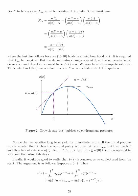
For F to be concave, Fxx must be negative if it exists. So we must have

Fxx =αFx

a(x)− u−(

αF − u

a(x)− u

)(a′(x)

a(x)− u

)

=

(αF − u

a(x)− u

)(α− a′(x)

a(x)− u

)

≃ α− a′(x)

a(x)− u(x)

where the last line follows because (13.10) holds in a neighbourhood of x. It is requiredthat Fxx be negative. But the denominator changes sign at x, so the numerator mustdo so also, and therefore we must have a′(x) = α. We now have the complete solution.The control in (13.8) has a value function F which satisfies the HJB equation.

xx

a(x)

umax

α = a′(x)

u = a(x)

Figure 2: Growth rate a(x) subject to environment pressures

Notice that we sacrifice long term yield for immediate return. If the initial popula-tion is greater than x then the optimal policy is to fish at rate umax until we reach xand then fish at rate u = a(x). As α ր a′(0), x ց 0. If α ≥ a′(0) then it is optimal towipe out the entire fish stock.

Finally, it would be good to verify that F (x) is concave, as we conjectured from thestart. The argument is as follows. Suppose x > x. Then

F (x) =

∫ T

0

umaxe−αtdt+

∫ ∞

T

a(x)e−αtdt

= a(x)/α+ (umax − a(x))(1− e−αT

)/α

58

where T = T (x) is the time taken for the fish population to decline from x to x, whenx = a(x)− umax. Now

T (x) = δ + T (x+ (a(x) − umax)δ) =⇒ 0 = 1 + (a(x)− umax)T′(x)

=⇒ T ′(x) = 1/(umax − a(x))

So F ′′(x) has the same sign as that of

d2

dx2

(1− e−αT

)= −αe−αT (α− a′(x))

(umax − a(x))2,

which is negative, as required, since α = a′(x) ≥ a′(x), when x > x. The case x < x issimilar.

59

14 Pontryagin’s Maximum Principle

Pontryagin’s maximum principle. Optimization of consumption. Parking a rocket car. Adjoint

variables as Lagrange multipliers.

14.1 Example: optimization of consumption

Suppose that given x(0), κ and T , all positive, we wish to choose u(t) to maximize∫ T

0

log u(t) dt+ κ logx(T ), subject to x(t) = ax(t) − u(t), 0 ≤ t ≤ T.

Solution. Try using a Lagrange multiplier λ(t) for the constraint x(t) = ax(t)− u(t).The Lagrangian is

L = κ logx(T ) +

∫ T

0

[log u− λ(x − (ax− u))]dt

Now use integration by parts, and define H(x, u, λ) = log u+ λ(ax− u).

L = κ log x(T )− λ(t)x(t)∣∣∣

T

0+

∫ T

0

[log u+ λx+ λ(ax − u)]dt

= [κ log x(T )− λ(T )x(T )] + λ(0)x(0) +

∫ T

0

[λx+H(x, u, λ)]dt.

To make L stationary with respect to both x(t) and u(t), at every point within theintegrand, we need

λ+∂

∂xH(x, u, λ) = 0 =⇒ λ = −aλ

∂

∂uH(x, u, λ) = 0 =⇒ u = 1/λ,

and so λ(t) = λ(0)e−at, u(t) = λ(0)−1eat and x(t) = ax(t) − λ(0)−1eat.If the value of x(T ) is prescribed (and < eaTx(0) so u need not be negative), then

we can solve this differential equation for x, choosing λ(0) so that x(t) takes prescribedvalues x(0) and x(T ) at t = 0 and T . We get (after some algebra)

u(t) =

(x(0)− x(T )e−aT

(T − t)x(0)− x(T )e−aT

)

x(t).

If the value of x(T ) is free, then stationarity of L with respect to x(T ) requiresκ/x(T )− λ(T ) = 0 which (after some algebra) implies λ(0) = (κ+ T )/x(0) and

u(t) =1

T + κx(0)eat =

1

(T − t) + κx(t).

If a > 1/(κ + T ) the trajectory is one in which x(t) is initially increasing and thendecreasing; otherwise x(t) is decreasing. The optimal ‘inheritance’ left at T is

x(T ) =κ

κ+ Tx(0)eaT .

60

14.2 Heuristic derivation of Pontryagin’s maximum principle

Pontryagin’s maximum principle (PMP) states a necessary condition that musthold on an optimal trajectory. It is a calculation for a fixed initial value of the state,x(0). In comparison, the dynamic programming approach is a calculation for a generalinitial value of the state. Thus, when PMP is useful, it finds an open-loop prescriptionof the optimal control, whereas dynamic programming is useful for finding a closed-loopprescription. PMP can be used as both a computational and analytic technique (andin the second case can solve the problem for general initial value.)

We begin by considering a time-homogeneous formulation, with plant equation x =a(x, u) and instantaneous cost c(x, u). The trajectory is to be controlled until it reachessome stopping set S, where there is a terminal costK(x). As in (13.6) the value functionF (x) obeys the a dynamic programming equation (without discounting)

infu∈U

[

c(x, u) +∂F

∂xa(x, u)

]

= 0, x 6∈ S, (14.1)

with terminal condition

F (x) = K(x), x ∈ S. (14.2)

Define the adjoint variable

λ = −Fx. (14.3)

This is a column n-vector, and is to be regarded as a function of time as the statemoves along the optimal trajectory. The proof that Fx exists in the required sense isactually a tricky technical matter. We also define the Hamiltonian

H(x, u, λ) = λ⊤a(x, u)− c(x, u), (14.4)

a scalar, defined at each point of the path as a function of the current x, u and λ.

Theorem 14.1. (PMP) Suppose u(t) and x(t) represent the optimal control and statetrajectory. Then there exists an adjoint trajectory λ(t) such that together u(t), x(t) andλ(t) satisfy

x = Hλ, [ = a(x, u) ] (14.5)

λ = −Hx, [ = −λ⊤ax + cx ] (14.6)

and for all t, 0 ≤ t ≤ T , and all feasible controls v,

H(x(t), v, λ(t)) ≤ H(x(t), u(t), λ(t)), (14.7)

i.e. the optimal control u(t) is the value of v maximizing H((x(t), v, λ(t)).

‘Proof.’ Our heuristic proof is based upon the DP equation; this is the most directand enlightening way to derive conclusions that may be expected to hold in general.

61

Assertion (14.5) is immediate, and (14.7) follows from the fact that the minimizingvalue of u in (14.1) is optimal. Assuming u is the optimal control we have from (14.1)in incremental form as

F (x, t) = c(x, u)δ + F (x+ a(x, u)δ, t+ δ) + o(δ).

Now use the chain rule to differentiate with respect to xi and this yields

d

dxiF (x, t) = δ

d

dxic(x, u) +

∑

j

∂

∂xjF (x+ a(x, u)δ, t+ δ)

d

dxi(xj + aj(x, u)δ)

=⇒ −λi(t) = δdc

dxi− λi(t+ δ)− δ

∑

j

λj(t+ δ)dajdxi

+ o(δ)

=⇒ d

dtλi(t) =

dc

dxi−∑

j

λj(t)dajdxi

which is (14.6).

Notice that (14.5) and (14.6) each give n equations. Condition (14.7) gives a furtherm equations (since it requires stationarity with respect to variation of them componentsof u.) So in principle these equations, if nonsingular, are sufficient to determine the2n+m functions u(t), x(t) and λ(t).

14.3 Example: parking a rocket car

A rocket car has engines at both ends. Initial position and velocity are x1(0) and x2(0).

0 x1

x2

By firing the rockets (causing acceleration of u in the forward or reverse direction) wewish to park the car in minimum time, i.e. minimize T such that x1(T ) = x2(T ) = 0.The dynamics are x1 = x2 and x2 = u, where u is constrained by |u| ≤ 1.

Let F (x) be minimum time that is required to park the rocket car. Then

F (x1, x2) = min−1≤u≤1

{

δ + F (x1 + x2δ, x2 + uδ)}

.

By making a Taylor expansion and then letting δ → 0 we find the HJB equation:

0 = min−1≤u≤1

{

1 +∂F

∂x1x2 +

∂F

∂x2u

}

(14.8)

62

with boundary condition F (0, 0) = 0. We can see that the optimal control will be abang-bang control with u = − sign( ∂F

∂x2) and so F satisfies

0 = 1 +∂F

∂x1x2 −

∣∣∣∣

∂F

∂x2

∣∣∣∣.

Now let us tackle the same problem using PMP. We wish to minimize

C =

∫ T

0

1 dt

where T is the first time at which x = (0, 0). For dynamics if x1 = x2, x2 = u, |u| ≤ 1,the Hamiltonian is

H = λ1x2 + λ2u− 1,

which is maximized by u = sign(λ2). The adjoint variables satisfy λi = −∂H/∂xi, so

λ1 = 0, λ2 = −λ1. (14.9)

Suppose that at termination λ1 = α, λ2 = β. Then in terms of time to go we cancompute

λ1 = α, λ2 = β + αs.

These reveal the form of the solution: there is at most one change of sign of λ2 on theoptimal path; u is maximal in one direction and then possibly maximal in the other.

From (14.1) or (14.8) we see that the maximized value of H must be 0. So attermination (when x2 = 0), we conclude that we must have |β| = 1. We now considerthe case β = 1. The case β = −1 is similar.

If β = 1, α ≥ 0 then λ2 = 1 + αs ≥ 0 for all s ≥ 0 and

u = 1, x2 = −s, x1 = s2/2.

In this case the optimal trajectory lies on the parabola x1 = x22/2, x1 ≥ 0, x2 ≤ 0. This

is half of the switching locus x1 = ±x22/2 (shown dotted in Figure 3).

If β = 1, α < 0 then u = −1 or u = 1 as the time to go is greater or less thans0 = 1/|α|. In this case,

u = −1, x2 = (s− 2s0), x1 = 2s0s− 12s

2 − s20, s ≥ s0,u = 1, x2 = −s, x1 = 1

2s2, s ≤ s0.

The control rule expressed as a function of s is open-loop, but in terms of (x1, x2) andthe switching locus, it is closed-loop.

63

a

b

x1

x2

u = 1

u = −1switching locus

Figure 3: Optimal trajectories for parking a rocket car. Notice that the trajectoriesstarting from two nearby points, a and b, are qualitatively different. From a we takefirst u = 1 then u = −1. From b we first take u = −1, then u = 1.

14.4 Adjoint variables as Lagrange multipliers

We have already seen in §14.1 that it is possible to think of λ(t) as a Lagrange multiplierfor the constraint x = a(x, u) (at time t). Consider the Lagrangian

L = −K(x(T )) +

∫ T

0

[−c− λ⊤(x− a)

]dt.

This is to be maximized over (x, u, λ) paths having the property that x(t) first entersthe set S at time T . We integrate λ⊤x by parts to obtain

L = −K(x(T ))− λ(T )⊤x(T ) + λ(0)⊤x(0) +

∫ T

0

[

λ⊤x+ λ⊤a− c]

dt.

We now think about varying both x(t) and u(t), but without regard to the constraintx = a(x, u). The quantity within the integral must be stationary with respect tox = x(t) and hence λ+ λ⊤ax − cx = 0 =⇒ λ = −Hx, i.e. (14.6).

If x(T ) is unconstrained then the Lagrangian must also be stationary with respectto small variations in x(T ) that are in a direction σ such that x(T ) + ǫσ is in thestopping set (or within o(ǫ) of it), and this gives (Kx(x(T )) + λ(T ))⊤σ = 0, i.e. theso-called transversality conditions, which we will say more about in (15.1).

It is good to have this alternative viewpoint, but it is informal and less easy torigorise than the ‘proofs’ of in §14.2, and §15.1

64

15 Using Pontryagin’s Maximum Principle

Transversality conditions. Examples with Pontryagin’s maximum principle.

15.1 Transversality conditions

In (14.1) we see that H must be maximized to 0. We can make this a generally validassertion, and also say some things about the terminal value of λ(T ) (the so-calledtransversality conditions.)

Theorem 15.1. (i) H = 0 on the optimal path. (ii) The terminal condition

(λ+Kx)⊤σ = 0 (15.1)

holds at the terminal x for all σ such that x+ ǫσ is within o(ǫ) of the termination pointof a possible optimal trajectory for all sufficiently small positive ǫ.

‘Proof.’ Assertion (i) follows from (14.1). To see (ii), suppose that x is a point atwhich the optimal trajectory first enters S. Then x ∈ S and so F (x) = K(x). Supposex+ ǫσ + o(ǫ) ∈ S. Then

0 = F (x+ ǫσ + o(ǫ))−K(x+ ǫσ + o(ǫ))

= F (x)−K(x) + (Fx(x)−Kx(x))⊤σǫ + o(ǫ)

Together with F (x) = K(x) this gives (Fx − Kx)⊤σ = 0. Since λ = −Fx we get

(λ+Kx)⊤σ = 0.

15.2 Example: use of transversality conditions

Suppose x1 = x2, x2 = u, x(0) = (0, 0), u is unconstrained, and we wish to minimize

C = −x1(1) +

∫ 1

0

12u(t)

2 dt.

Here K(x) = −x1(1). The Hamiltonian is

H(x, u, λ) = λ1x2 + λ2u− 12u

2,

which is maximized at u(t) = λ2(t). Now λi = −∂H/∂xi gives

λ1 = 0, λ2 = −λ1.

The terminal x is unconstrained so in the transversality condition of (λ+Kx)⊤σ = 0,

σ is arbitrary and so we also have

λ1(1)− 1 = 0, λ2(1) = 0.

Thus the solution must be λ1(t) = 1 and λ2(t) = 1 − t. The optimal control isu(t) = 1− t.

Note that there is often more than one way to set up a control problem. In this

problem, we might have takenK = 0, but included a cost of−∫ 1

0x2 dt = −x1(1)+x1(0).

65

15.3 Example: insects as optimizers

A colony of insects consists of workers and queens, of numbers w(t) and q(t) at time t.If a time-dependent proportion u(t) of the colony’s effort is put into producing workers,(0 ≤ u(t) ≤ 1, then w, q obey the equations

w = auw − bw, q = c(1− u)w,

where a, b, c are constants, with a > b. The function u is to be chosen to maximize thenumber of queens at the end of the season. Show that the optimal policy is to produceonly workers up to some moment, and produce only queens thereafter.

Solution. In this problem the Hamiltonian is

H = λ1(auw − bw) + λ2c(1 − u)w

and K(w, q) = −q. The adjoint equations and transversality conditions give

−λ1 = Hw = λ1(au− b) + λ2c(1− u)

−λ2 = Hq = 0,

λ1(T ) = −Kw = 0λ2(T ) = −Kq = 1

,

and hennce λ2(t) = 1 for all t. Since H is maximized by u,

u =01

if ∆(t) := λ1a− c<>

0.

Since ∆(T ) = −c, we must have u(T ) = 0. If t is a little less than T , λ1 is small andu = 0 so the equation for λ1 is

λ1 = λ1b− c. (15.2)

As long as λ1 is small, λ1 < 0. Therefore as the remaining time s increases, λ1(s)increases, until such point that ∆(t) = λ1a−c ≥ 0. The optimal control becomes u = 1and then λ1 = −λ1(a − b) < 0, which implies that λ1(s) continues to increase as sincreases, right back to the start. So there is no further switch in u.

The point at which the single switch occurs is found by integrating (15.2) from t toT , to give λ1(t) = (c/b)(1− e−(T−t)b) and so the switch occurs where λ1a− c = 0, i.e.(a/b)(1− e−(T−t)b) = 1, or

tswitch = T + (1/b) log(1− b/a).

Experimental evidence suggests that social insects do closely follow this policy andadopt a switch time that is nearly optimal for their natural environment.

15.4 Problems in which time appears explicitly

Thus far, c(·), a(·) and K(·) have been function of (x, u), but not t. Sometimes wewish to solve problems in t appears, such as when x = a(x, u, t). We can cope with this

66

generalization by the simple mechanism of introducing a new variable that equates totime. Let x0 = t, with x0 = a0 = 1.

Having been augmented by this variable, the Hamiltonian gains a term and becomes

H = λ0a0 +H = λ0a0 +n∑

i=1

λiai − c

where λ0 = −Ft and a0 = 1. Theorem 15.1 says that H must be maximized to 0.Equivalently, on the optimal trajectory,

H(x, u, λ) =

n∑

i=1

λiai − c must be maximized to − λ0.

Theorem 14.1 still holds. However, to (14.6) we can now add

λ0 = −Ht = ct − λat, (15.3)

and transversality condition

(λ +Kx)⊤σ + (λ0 +Kt)τ = 0, (15.4)

which must hold at the termination point (x, t) if (x + ǫσ, t + ǫτ) is within o(ǫ) of thetermination point of an optimal trajectory for all small enough positive ǫ.

We can now understand what to do with various types of time-dependancy and ter-minal conditions on x(T ) and/or T . For example, we can draw the following inferences.

(i) If K is time-independent (so Kt = 0) and the terminal time T is unconstrained(so τ is arbitrary) then the transversality condition implies λ0(T ) = 0. Since His always maximized to −λ0(t) it must be maximized to 0 at T .

(ii) If a, c are only functions of (x, u) then λ0 = ct − λ⊤at = 0, and so λ0(t) isconstant on the optimal trajectory. Since H is always maximized to −λ0(t) itmust be maximized to a constant on the optimal trajectory.

(iii) If both (i) and (ii) are true then H is maximized to 0 along the entire optimaltrajectory. We had this in the problem of parking in minimal time, §14.3.

15.5 Example: monopolist

Miss Prout holds the entire remaining stock of Cambridge elderberry wine for thevintage year 1959. If she releases it at rate u (in continuous time) she realises a unitprice p(u) = (1 − u/2), for 0 ≤ u ≤ 2 and p(u) = 0 for u ≥ 2. She holds an amount xat time 0 and wishes to release it in a way that maximizes her total discounted return,∫ T

0e−αtup(u) dt, (where T is unconstrained.)

67

Solution. Notice that t appears in the cost function. The plant equation is x = −uand the Hamiltonian is

H(x, u, λ) = e−αtup(u)− λu = e−αtu(1− u/2)− λu.

Note that K = 0. Maximizing with respect to u and using λ = −Hx gives

u = 1− λeαt, λ = 0, t ≥ 0,

so λ is constant. The terminal time is unconstrained so the transversality condition givesλ0(T ) = −Kt|t=T = 0. Therefore, since we require H to be maximized to −λ0(T ) = 0at T , we have u(T ) = 0, and hence

λ = e−αT , u = 1− e−α(T−t), t ≤ T,

where T is then the time at which all wine has been sold, and so

x =

∫ T

0

u dt = T −(1− e−αT

)/α.

Thus u is implicitly a function of x, through T .

0.5 1.0 1.5 2.0 2.5 3.0

0.2

0.4

0.6

0.8

1.0

x(t)

u(t)

Figure 4: Trajectories of x(t), u(t), for α = 1.

The optimal value function is

F (x) =

∫ T

0

(u− u2/2)e−αt dt =1

2

∫ T

0

(e−αt − eαt−2αT

)dt =

(1− e−αT

)2

2α.

15.6 Example: neoclassical economic growth

Suppose x is the existing capital per worker and u is consumption of capital per worker.The plant equation is

x = f(x)− γx− u, (15.5)

where f(x) is production per worker (which depends on capital available to the worker),and −γx represents depreciation of capital. We wish to choose u to maximize

∫ T

t=0

e−αtg(u)dt,

68

where g(u) measures utility and T is prescribed.

Solution. This is really the same as the fish harvesting example in §13.5, with a(x) =f(x)− γx. So let us take

x = a(x)− u. (15.6)

It is convenient to takeH = e−αt [g(u) + λ(a(x) − u)]

so including a discount factor in the definition of u, corresponding to expression of Fin terms of present values. Here λ is a scalar. Then g′(u) = λ (assuming the maximumis at a stationary point), and

d

dt

(e−αtλ

)= −Hx = −e−αtλa′(x) (15.7)

orλ(t) = (α − a′(x))λ(t). (15.8)

From g′(u) = λ we have g′′(u)u = λ and hence from (15.8) we obtain

u =1

σ(u)[a′(x)− α], (15.9)

where

σ(u) = −g′′(u)

g′(u)

is the elasticity of marginal utility. Assuming g is strictly increasing and concave wehave σ > 0. So (x, u) are determined by (15.6) and (15.9). An equilibrium solution atx, u is determined by

u = a(x) a′(x) = α,

These give the balanced growth path; interestingly, it is independent of g.

This provides an example of so-called turnpike theory. For sufficiently large T theoptimal trajectory will move from the initial x(0) to within an arbitrary neighbourhoodof the balanced growth path (the turnpike) and stay there for all but an arbitrarily smallfraction of the time. As the terminal time becomes imminent the trajectory leaves theneighbourhood of the turnpike and heads for the terminal point x(T ) = 0.

69

16 Controlled Diffusion Processes

Control problems in a continuous-time, continuous state space, stochastic setting.

16.1 The dynamic programming equation

The DP equation in incremental form is

F (x, t) = infu{c(x, u)δt+ E[F (x(t+ δt), t+ δt) | x(t) = x, u(t) = u)]}.

If appropriate limits exist then this can be written in the limit δt ↓ 0 as

infu[c(x, u) + Ft(x, t) + Λ(u)F (x, t)] = 0.

Here Λ(u) is the operator defined by

Λ(u)φ(x) = limδt↓0

[E[φ(x(t + δt)) | x(t) = x, u(t) = u]− φ(x)

δt

]

(16.1)

or

Λ(u)φ(x) = limδt↓0

E

[φ(x(t + δt))− φ(x)

δt

∣∣∣∣x(t) = x, u(t) = u

]

the conditional expectation of the ‘rate of change’ of φ(x) along the path. The operatorΛ converts a scalar function of state, φ(x), to another such function, Λφ(x). However, itsaction depends upon the control u, so we write it as Λ(u). It is called the infinitesimalgenerator of the controlled Markov process. Equation (16.1) is equivalent to

E[φ(x(t + δt) | x(t) = x, u(t) = u] = φ(x) + Λ(u)φ(x)δt + o(δt).

This equation takes radically different forms depending upon whether the state spaceis discrete or continuous. Both are important.

If the state space is discrete we have the Markov jump process of Lecture 9. In thiscase Λ(u)φ(i) =

∑

j qij(u)[φ(j) − φ(i)]. Now we turn to the case of continuous statespace.

16.2 Diffusion processes and controlled diffusion processes

The Wiener process {B(t)}, is a scalar process for which B(0) = 0, the incrementsin B over disjoint time intervals are statistically independent and B(t) is normallydistributed with zero mean and variance t. (‘B’ stands for Brownian motion. It canbe understood as a δ → 0 limit of a symmetric random walk in which steps ±

√δ are

made at times δ, 2δ, . . . .) The specification is internally consistent because, for example,

B(t) = B(t1) + [B(t)−B(t1)]

and for 0 ≤ t1 ≤ t the two terms on the right-hand side are independent normalvariables of zero mean and with variance t1 and t− t1 respectively.

70

If δB is the increment of B in a time interval of length δt then

E(δB) = 0, E[(δB)2] = δt, E[(δB)j ] = o(δt), for j > 2,

where the expectation is one conditional on the past of the process. Note that since

E[(δB/δt)2] = O[(δt)−1

]→ ∞,

the formal derivative ǫ = dB/dt (continuous-time ‘white noise’) does not exist in amean-square sense, but expectations such as

E

[{∫

α(t)ǫ(t)dt

}2]

= E

[{∫

α(t)dB(t)

}2]

=

∫

α(t)2dt

make sense if the integral is convergent.Now consider a stochastic differential equation

δx = a(x, u)δt+ g(x, u)δB,

which we shall write formally as

x = a(x, u) + g(x, u)ǫ.

This, as a Markov process, has an infinitesimal generator with action

Λ(u)φ(x) = limδt↓0

E

[φ(x(t + δt))− φ(x)

δt

∣∣∣∣x(t) = x, u(t) = u

]

= φxa+12φxxg

2

= φxa+12Nφxx,

where N(x, u) = g(x, u)2. So in the scalar case this controlled diffusion process hasDP equation

infu

[c+ Ft + Fxa+ 1

2NFxx

]= 0, (16.2)

and in the vector case

infu

[c+ Ft + F⊤

x a+ 12 tr(NFxx)

]= 0.

16.3 Example: noisy LQ regulation in continuous time

The dynamic programming equation is

infu

[x⊤Rx+ u⊤Qu+ Ft + F⊤

x (Ax+Bu) + 12 tr(NFxx)

]= 0.

In analogy with the discrete and deterministic continuous cases that we have consideredpreviously, we try a solution of the form,

F (x, t) = x⊤Π(t)x + γ(t).

71

This leads to the same Riccati equation as in Section 13.4,

0 = x⊤

[

R+ΠA+A⊤Π−ΠBQ−1B⊤Π+dΠ

dt

]

x,

and also, as in Section 10.3,

dγ

dt+ tr(NΠ(t)) = 0, giving γ(t) =

∫ T

t

tr(NΠ(τ)) dτ.

16.4 Example: passage to a stopping set

Consider a problem of movement on the unit interval 0 ≤ x ≤ 1 in continuous time,x = u + ǫ, where ǫ is white noise of power v. The process terminates at time T whenx reaches one end or the other of the the interval. The cost is made up of an integral

term 12

∫ T

0(L + Qu2)dt, penalising both control and time spent, and a terminal cost

which takes the value C0 or C1 according as termination takes place at 0 or 1.Show that in the deterministic case v = 0 one should head straight for one of the

termination points at a constant rate and that the value function F (x) has a piecewiselinear form, with possibly a discontinuity at one of the boundary points if that boundarypoint is the optimal target from no interior point of the interval.

Show, in the stochastic case, that the dynamic programming equation with thecontrol value optimized out can be linearised by a transformation F (x) = α logφ(x) fora suitable constant α, and hence solve the problem.

Solution. In the deterministic case the optimality equation is

infu

[L+Qu2

2+ u

∂F

∂x

]

= 0, 0 < x < 1, (16.3)

with boundary conditions F (0) = C0, F (1) = C1. If one goes (from x) for x = 0 atspeed w one incurs a cost of C0 + (x/2w)(L +Qw2) with a minimum over w value ofC0 + x

√LQ. Indeed (16.3) is solved by

F (x) = min[

C0 + x√

LQ,C1 + (1− x)√

LQ]

.

The minimizing option determines the target and the optimal w is√

L/Q.In the stochastic case

infu

[L+Qu2

2+ u

∂F

∂x+

v

2

∂2F

∂x2

]

= 0.

So u = −Q−1Fx and

L−Q−1

(∂F

∂x

)2

+ v∂2F

∂x2= 0.

72

Make the transform F (x) = −Qv logφ(x) so φ(x) = e−F (x)/Qv. Then the above equa-tion simplifies to

Qv2∂2φ

∂x2− Lφ = 0,

with solutionφ(x) = k1 exp

(x

v

√

L/Q)

+ k2 exp(

−x

v

√

L/Q)

.

We choose the constants k1, k2 to meet the two boundary conditions on F .

0 0.2 0.4 0.6 0.81

1

1.2

1.4

1.6

1.8

2.0

2.2

v = 1

v = 2

v = 0.5

v = 0.25

v = 0.125

Figure 5: F (x) against x for the passage to a stopping set

The figure shows the solution for L = 1, Q = 4, C0 = 1, C1 = 1.5 and v = 0.125, 0.25,0.5, 1, 2 and the deterministic solution.

Notice that for these parameter choices the presence of noise actually reduces cost.This is because we are nearly indifferent as to which endpoint we hit, and L is smallrelative to Q. So it will be good to keep u small and let the noise do most of the workin bringing the state to endpoint.

73