partially separable convexly-constrained optimization … · partially separable...
TRANSCRIPT
Partially separable convexly-constrained optimization
with non-Lipschitzian singularities and its complexity
X. Chen∗ Ph. L. Toint† and H. Wang‡
19 April 2017
Abstract
An adaptive regularization algorithm using high-order models is proposed for partiallyseparable convexly constrained nonlinear optimization problems whose objective functioncontains non-Lipschitzian `q-norm regularization terms for q ∈ (0, 1). It is shown that thealgorithm using an p-th order Taylor model for p odd needs in general at most O(ε−(p+1)/p)evaluations of the objective function and its derivatives (at points where they are defined)to produce an ε-approximate first-order critical point. This result is obtained eitherwith Taylor models at the price of requiring the feasible set to be ’kernel-centered’ (whichincludes bound constraints and many other cases of interest), or for non-Lipschitz models,at the price of passing the difficulty to the computation of the step. Since this complexitybound is identical in order to that already known for purely Lipschitzian minimizationsubject to convex constraints [9], the new result shows that introducing non-Lipschitziansingularities in the objective function may not affect the worst-case evaluation complexityorder. The result also shows that using the problem’s partially separable structure (ifpresent) does not affect complexity order either. A final (worse) complexity bound isderived for the case where Taylor models are used with a general convex feasible set.
Keywords: complexity theory, nonlinear optimization, non-Lipschitz function, `q-norm regular-
ization, partially separable problems.
1 Introduction
We consider the partially separable convexly constrained nonlinear optimization problem:
minx∈F
f(x) =∑i∈N
fi(Uix) +∑i∈H|Uix|q =
∑i∈N
fi(xi) +∑i∈H
fi(xi) (1.1)
where F is a non-empty closed convex set, N ∪H def= M, N ∩H = ∅, fi : IRn → IR, q ∈ (0, 1),
fi(xi) = |xi|q = |Uix|q for i ∈ H and where, for i ∈ M, xidef= Uix with Ui a (fixed) ni × n
∗Department of Applied Mathematics, The Hong Kong Polytechnic University, Hong Kong. Email:[email protected]†Namur Center for Complex Systems (naXys) and Department of Mathematics, University of Namur, 61,
rue de Bruxelles, B-5000 Namur, Belgium. Email: [email protected]‡Department of Applied Mathematics, The Hong Kong Polytechnic University, Hong Kong. Email:
1
Chen, Toint, Wang: Evaluation complexity of non-Lipschitzian optimization 2
matrix with ni ≤ n. Without loss of generality, we assume that ‖Ui‖ = 1 for all i ∈ M andthat the ranges of the UTi for i ∈ N span IRn in that the intersection of the nullspaces of theUi is reduced to the origin(1). In what follows, the “element functions” fi (i ∈ N ) will be“well-behaved” smooth functions with Lipschitz continuous derivatives(2). If H 6= ∅, we alsorequire that
ni = 1 (1.2)
and (initially at least(3)) that the feasible set is ’kernel centered’, in the sense that, if PX [·] isthe orthogonal projection ont the convex set X , then, for i ∈ H,
Pker(Ui)[F ] ⊆ F whenever ker(Ui) ∩ F 6= ∅ (1.3)
in addition of F being convex, closed and non-empty. As will be discussed below (afterLemma 4.2), we may assume without loss of generality that, ker(Ui) ∩ F 6= ∅ (and thusPker(Ui)[F ] ⊆ F) for all i ∈ H. ’Kernel centered’ feasible sets include boxes (corresponding tobound constrained problems), spheres/cylinders centered at the origin and other sets such as{
(x1, x2) ∈ IRn1+1 | x1 ∈ F1 and g1(x1) ≤ x2 ≤ −g2(x1)}, H = {2}, (1.4)
where F1 is a non-empty closed convex set in IRn1 and gi(·) are convex functions from IRn1 toIR (i = 1, 2, n1 + 1 ≤ n) such that gi(x1) ≤ 0 (i = 1, 2) for x1 ∈ F1. Compositions using (1.4)recursively, rotations, cartesian products or intersections of such sets are also kernel-centered.
Problem (1.1) has many applications in engineering and science. Using the non-Lipschitzregularization function in the second term of the objective function f has remarkable advan-tages for the restoration of piecewise constant images and sparse signals [1,4,28], and sparsevariable selection, for instance in bioinformatics [14, 27]. Theory and algorithms for solvingq-norm regularized optimization problems have been developed in [12,15,29].
The partially separable structure defined in problem (1.1) is ubiquitous in applications ofoptimization. It is most useful in the frequent case where ni � n and subsumes that of sparseoptimization (in the special case where the rows of each Ui are selected rows of the identitymatrix). Moreover the decomposition in (1.1) has the advantage of being invariant for linearchanges of variables (only the Ui matrices vary).
Partially separable optimization was proposed by Griewank and Toint in [26], studiedfor more than thirty years (see [10, 11, 20, 21, 30] for instance) and extensively used in thepopular CUTE(st) testing environment [23] as well as in the AMPL [19], LANCELOT [17] andFILTRANE [24] packages, amongst others. In particular, the design of trust-region algorithm-s exploiting the partially separable decomposition (1.1) was investigated by Conn, Gould,Sartenaer and Toint in [16,18] and Shahabuddin [33].
Focussing now on the nice multivariate element functions (i ∈ N ), we note that using thepartially separable nature of a function f can be very useful if one wishes to use derivativesof
fN (x)def=∑i∈N
fi(Uix) =∑i∈N
fi(xi) (1.5)
(1)If the {UTi }i∈N do not span IRn, problem (1.1) can be modified without altering its optimal value byintroducing an additional identically zero element term f0(U0x) (say) in N with associated U0 such that∩i∈N ker(Ui) ⊆ range(UT0 ). It is clear that, since f0(x0) = 0, it is differentiable with Lipschitz continuousderivative for any order p ≥ 1. Obviously, this covers the case where N = ∅ 6= H.
(2)Hence the symbol N for “nice”.(3)We will drop this assumption in Section 5.
Chen, Toint, Wang: Evaluation complexity of non-Lipschitzian optimization 3
of order larger than one in the context of the p-th order Taylor series
TfN ,p(x, s) = fN (x) +
p∑j=1
1
j!∇jxfN (x)[s]j . (1.6)
Indeed, it may be verified that
∇jxfN (x)[s]j =∑i∈N∇jxifi(xi)[Uis]
j . (1.7)
This last expression indicates that only the |N | tensors {∇jxifi(xi)}i∈N of dimension nji needs
to be computed and stored, a very substantial gain compared to the nj-dimensional ∇jxfN (x)when (as is common) ni � n for all i. It may therefore be argued that exploiting derivativetensors of order larger than 2 — and thus using the high-order Taylor series (1.6) as a localmodel of f(x + s) in the neighbourhood of x — may be practically feasible if f is partiallyseparable. Of course the same comment applies to
fH(x)def=∑i∈H
fi(Uix) =∑i∈H
fi(xi) (1.8)
whenever the required derivatives of fi(xi) = |xi|p (i ∈ H) exist.Interestingly, the use of high-order Taylor models for optimization was recently inves-
tigated by Birgin et al. [3] in the context of adaptive regularization algorithms for uncon-strained problems. Their proposal belongs to this emerging class of methods pioneered byGriewank [25], Nesterov and Polyak [32] and Cartis, Gould and Toint [6, 7] for the uncon-strained case and by these last authors in [8] for the convexly constrained case of interest here.Such methods are distinguished by their excellent evaluation complexity, in that they needat most O(ε−(p+1)/p) evaluations of the objective function and their derivatives to producean ε-approximate first-order critical point, compared to the O(ε−2) evaluations which mightbe necessary for the steepest descent and Newton’s methods (see [31] and [5] for details).However, most adaptive regularization methods rely on a non-separable regularization termin the model of the objective function, making exploitation of structure difficult(4).
The purpose of the present paper is twofold. Its first aim is to show that worst-caseevaluation complexity for nonconvex minimization subject to convex constraints is not affectedby the introduction of non-Lipschitzian singularities in the objective function. The secondand concurrent one is to show that this complexity is not affected either by the use of partiallyseparable structure, if present in the problem.
The remaining of the paper is organized as follows. Section 2 establishes a necessaryfirst-order optimality condition for the non-Lipschitzian case. Section 3 then introduces thepartially separable adaptive regularization algorithm for this problem while Section 4 is de-voted to its worst-case evaluation complexity analysis for the case where Taylor models areused with a kernel-centered feasible set. Section 5 drops the kernel-centered assumption fornon-Lipschitz models and Taylor models. The results are discussed in Section 6 and somefinal conclusions and perspectives are presented in Section 7.Notations. In what follow, ‖x‖ denotes the Euclidean norm of the vector x and ‖T‖p therecursively induced Euclidean norm on the p-th order tensor T (see [3, 9] for details). Thenotation T [s]i means that the tensor T is applied to i copies of the vector s. For any set X ,|X | denotes its cardinality. For any I ⊆M, we also denote fI(x) =
∑i∈I fi(x).
(4)The only exception we are aware of is the unpublished note [22] in which a p-th order Taylor model iscoupled with a regularization term involving the (totally separable) q-th power of the q norm (q ≥ 1).
Chen, Toint, Wang: Evaluation complexity of non-Lipschitzian optimization 4
2 First-order necessary conditions
In this section, we first present exact and approximate first-order necessary conditions fora local minimizer of problem (1.1). Such conditions for optimization problems with non-Lipschitzian singularities have been independently defined in the scaled form [15] or in sub-spaces [2, 14]. In a recent paper [13], KKT necessary optimality conditions for constrainedoptimization problems with non-Lipschitzan singularities are studied under the relaxed con-stant positive linear dependence and basic qualification. The above optimality conditionstake the singularity into account by no longer requiring that the gradient (for unconstrainedproblems, say) nearly vanishes at an approximate solution xε (which would be impossible ifthe singularity is active) but by requiring that a scaled version of this requirement holds inthat ‖Xε∇1
xf(xε)‖ is suitably small, where Xε is a diagonal matrix whose diagonal entries arethe components of xε. Unfortunately, if the i-th component of xε is small but not quite smallenough to consider that the singularity is active for variable i (say it is equal to 2ε), the i-thcomponent of ∇1
xf(x) can be as large as a multiple of ε−1. As a result, comparing worst-caseevaluation complexity bounds with those known for purely Lipschitz continuous problems(such as those proposed in [3] or [9]) may be misleading, since these latter conditions wouldnever accept an approximate first-order critical point with such a large gradient. In order toavoid these pitfalls, we now propose a stronger definition of approximate first-order criticalpoint for non-Lipschitzian problems where such “border-line” situations do not occur. Thenew definition is also makes use of subspaces but exactly reduces to the standard conditionfor Lipschitzian problems if the singularity is not active at xε, even if it is close to it.
Given a vector x ∈ IRn and ε ≥ 0, denote
C(x, ε) def= {i ∈ H | |Uix| ≤ ε}, R(x, ε)
def=
⋂i∈C(x,ε)
ker(Ui) =
[spani∈C(x,ε)
{UTi }
]⊥
andW(x, ε)
def= N ∪ (H \ C(x, ε)).
For convenience, if ε = 0, we denote C(x)def= C(x, 0), R(x)
def= R(x, ε) and W(x)
def=
W(x, 0).Observe that the definition of R(x, ε) above gives that
R(x, ε)⊥ ⊆ spani∈H{UTi }. (2.1)
Also note that any x ∈ IRn can be decomposed uniquely as x = y + z where y ∈ R(x)⊥ andz ∈ R(x). By the definition of R(x), it is not difficult to verify that
Uiz = 0, ∀i ∈ C(x) and x ∈ R(x).
Finaly note that, although f(x) is nonsmooth if H 6= ∅, fW(x,ε)(x) is as differentiable as thefi(x) for i ∈ N and any ε ≥ 0. This allows us to formulate our first-order necessary condition.
Chen, Toint, Wang: Evaluation complexity of non-Lipschitzian optimization 5
Theorem 2.1 If x∗ ∈ F is a local minimizer of problem (1.1), then
χf (x∗) = 0, (2.2)
where, for any x ∈ F ,
χf (x∗) = χf (x∗, 0)def=
∣∣∣∣∣∣∣ minx+d∈F
d∈R(x),‖d‖≤1
∇1xfW(x)(x)Td
∣∣∣∣∣∣∣ . (2.3)
Proof. Suppose first thatR(x∗) = {0} (which happens if x∗ = 0 ∈ F and spani∈H{UTi } =IRn). Then (2.2)-(2.3) holds vacuously. Now suppose that R(x∗) contains at least onenonzero element. By assumption, there exists δx∗ > 0 such that
f(x∗) = min{fN (x) + fH(x) | x ∈ F , ‖x− x∗‖ ≤ δx∗}= min{fN (y + z) + fH(y + z) | y + z ∈ F , y ∈ R(x∗)
⊥, z ∈ R(x∗), ‖y + z − x∗‖ ≤ δx∗}
≤ min{fN (y + z) +∑i∈H|Ui(y + z)|q | y + z ∈ F , y = 0, z ∈ R(x∗), ‖z − x∗‖ ≤ δx∗}
= min{fN (z) +∑i∈H|Uiz|q | z ∈ F ∩R(x∗), ‖z − x∗‖ ≤ δx∗}
= min{fN (z) +∑
i∈H\C(x∗)
|Uiz|q | z ∈ F ∩R(x∗), ‖z − x∗‖ ≤ δx∗}.
We now introduce a new problem, which is problem (1.1) reduced to R(x∗), namely,
min fW(x∗)(z) = fN (z) +∑
i∈H\C(x∗)
|Uiz|q,
s.t. z ∈ F ∩R(x∗)
(2.4)
where the gradient ∇1zfW(x∗)(z) is locally Lipschitz continuous in some (bounded) neigh-
borhood of x∗. It then follows from x∗ ∈ R(x∗) that
fW(x∗)(x∗) = fN (x∗) +∑
i∈H\C(x∗)
|Uix∗|q = f(x∗).
Therefore, we have that
fW(x∗)(x∗) ≤ min{fW(x∗)(z) | z ∈ F ∩ C(x∗), ‖z − x∗‖ ≤ δx∗}
which implies that x∗ is a local minimizer of problem (2.4). Hence, we have
∇1zfW(x∗)(x∗)
T (z − x∗) ≥ 0, z ∈ F ∩R(x∗). (2.5)
In addition,
{d = 0} ⊆ {d | x∗ + d ∈ F , d ∈ R(x∗), ‖d‖ ≤ 1} ⊆ {d | x∗ + d ∈ F , d ∈ R(x∗)}
which gives the desired result (2.2)-(2.3). 2
Chen, Toint, Wang: Evaluation complexity of non-Lipschitzian optimization 6
We call x∗ a first-order stationary point of (1.1), if x∗ satisfies the relation (2.2) in Theorem 2.1.For ε > 0, we call xε an ε-approximate first-order stationary point of (1.1), if xε satisfies
χf (xε, ε)def=
∣∣∣∣∣∣∣ minx+d∈F
d∈R(xε,ε),‖d‖≤1
∇1xfW(xε,ε)(xε)
Td
∣∣∣∣∣∣∣ ≤ ε. (2.6)
Theorem 2.2 Let xε be an ε-approximate first-order stationary point of (1.1). Thenany cluster point of {xε}ε>0 is a first-order stationary point of problem (1.1) as ε→ 0.
Proof. Suppose that x∗ is any cluster point of {xε}ε>0. Hence there must exist aninfinite sequence {εk} converging to zero and an infinite sequence {xεk}k≥0 ⊆ {xε}ε>0
such that x∗ = limk→∞ xεk and xεk is an εk-approximate first-order stationary point of(1.1) for eack k ≥ 0. If R(x∗) = {0}, (2.2) holds vacuously and hence x∗ is a first-orderstationary point. Suppose therefore that R(x∗) contains at least one nonzero element,implying that the dimension of R(x∗) is strictly positive.
First of all, we claim that there must exist k∗ ≥ 0 such that R(xεk , εk)⊥ ⊆ R(x∗)
⊥ for anyk ≥ k∗. Indeed, if that is not the case, there exists a subsequence of {xεk}, say {xεkj }, such
that limj→∞ εkj = 0 and R(xεkj , εkj )⊥ 6⊆ R(x∗)
⊥ for all j. Using now (2.1) and the fact
that H is a finite set, we obtain that there must exist an i0 ∈ H such that i0 ∈ C(xεkjt , εkjt )but i0 /∈ C(x∗) where {kjt} ⊆ {kj} with t = 1, 2, · · · . For convenience, we continue to use{kj} to denote its subsequence {kjt}. Hence, we have that
|Ui0xεkj | ≤ εkj .
Let j go to infinity. It then follows from the above inequality that |Ui0x∗| = 0, whichcontradicts the fact that i0 /∈ C(x∗). Thus, we conclude that, for some k∗ ≥ 0 and allk ≥ k∗, R(xεk , εk)
⊥ ⊆ R(x∗)⊥. Therefore we have that R(x∗) ⊆ R(xεk , εk) for k ≥ k∗.
For any fixed εk approximate first-order stationary point xεk , consider the following twominimization problems.
min ∇1xfW(xεk ,εk)
(xεk)Td,
s.t. xεk + d ∈ F , d ∈ R(xεk , εk), ‖d‖ ≤ 1,(2.7)
and
min ∇1xfW(xεk ,εk)
(xεk)Td,
s.t. xεk + d ∈ F , d ∈ R(x∗), ‖d‖ ≤ 1.(2.8)
Since d = 0 is a feasible point of both problems (2.7) and (2.8), the minimum values of(2.7) and (2.8) are both nonpositive. Moreover, it follows from R(x∗) ⊆ R(xεk , εk) thatthe minimum value of (2.8) is not smaller than that of (2.7).
Chen, Toint, Wang: Evaluation complexity of non-Lipschitzian optimization 7
Hence, from (2.6), we have that for any xεk ,∣∣∣∣∣∣∣∣ minxεk+d∈F
d∈R(x∗),‖d‖≤1
∇1xfW(xεk ,εk)
(xεk)Td
∣∣∣∣∣∣∣∣ ≤∣∣∣∣∣∣∣∣ min
xεk+d∈Fd∈R(xεk ,εk),‖d‖≤1
∇1xfW(xεk ,εk)
(xεk)Td
∣∣∣∣∣∣∣∣ ≤ εk. (2.9)
Suppose that dεk is a minimizer of problem (2.8), then (2.9) implies that
−εk ≤ ∇1xfW(xεk ,εk)
(xεk)Tdεk ≤ 0, (2.10)
where dεk should satisfy that xεk + dεk ∈ F , dεk ∈ R(x∗) and ‖dεk‖ ≤ 1. Note that, sincedεk ∈ R(x∗),
∇1xfW(xεk ,εk)
(xεk)Tdεk =
∇xfN (xεk) +∑
i∈H\C(xεk )
q|Uixεk |q−1sign(Uixεk)UTi
T
dεk
= ∇xfN (xεk)Tdεk +∑
i∈H\C(xεk )
q|Uixεk |q−1sign(Uixεk)Uidεk
= ∇xfN (xεk)Tdεk +∑i∈H
q|Uixεk |q−1sign(Uixεk)Uidεk .
(2.11)
From the compactness of {d | ‖d‖ ≤ 1}, we know that there must exist a subsequenceof {dεk} such that dεkj → d∗ ∈ R(x∗) with ‖d∗‖ ≤ 1 as j goes to infinity. Since for
i ∈ H\C(x∗), we have limk→∞ |Uixεk |q−1 = |Uix∗|q−1. Let k go to infinity in (2.10) and(2.11), and we obtain that
0 = ∇1xfW(xεk ,εk)
(x∗)Td∗ = ∇fN (x∗)
Td∗ +∑
i∈H\C(x∗)
q|Uix∗|q−1sign(Uix∗)Uid∗,
which implies that
minx∗+d∈F
d∈R(x∗),‖d‖≤1
∇1xfW(xεk ,εk)
(x∗)Td = ∇1
xfW(x∗)(x∗)Td∗ = 0
and completes the proof. 2
3 A partially separable regularization algorithm
We now examine the desired properties of the element functions fi more closely. Assumefirst that, for i ∈ N , each element function fi is p times continuously differentiable and itsp-th order derivative tensor ∇pxfi is globally Lipschitz continuous with constant Li ≥ 0 in thesense that, for all xi, yi ∈ range(Ui),
‖∇pxifi(xi)−∇pxifi(yi)‖p ≤ Li‖xi − yi‖. (3.1)
Chen, Toint, Wang: Evaluation complexity of non-Lipschitzian optimization 8
It can be shown (see (4.6) below) that this assumption implies that, for i ∈ N ,
fi(xi + si) = Tfi,p(xi, si) +1
(p+ 1)!τiLi‖si‖p+1 with |τi| ≤ 1, (3.2)
where si = Uis.Because the quantity τiLi in (3.2) is usually unknown in practice, it is impossible to use
(3.2) directly to model the objective function in a neighbourhood of x. However, we mayreplace this term with an adaptive parameter σi, which yields the following (p+ 1)-th ordermodel for the i-th element (i ∈ N ):
mi(xi, si) = Tfi,p(xi, si) +1
(p+ 1)!σi‖si‖p+1. (3.3)
There is more than one possible choice for defining the element models for i ∈ H. Thefirst(5) is to pursue the line of polynomial Taylor-based models, for which we need the followingtechnical result.
Lemma 3.1 We have that, for i ∈ H and all x, s ∈ IRn with Uix 6= 0 6= Ui(x+ s),
|xi + si|q = |xi|q + q
∞∑j=1
1
j!
(j−1∏`=1
(q − `)
)|xi|q−jµ(xi, si)
j , (3.4)
where
µ(xi, si)def=
si if xi > 0 and xi + si > 0,−si if xi < 0 and xi + si < 0,−(2xi + si) if xi > 0 and xi + si < 0,
2xi + si if xi < 0 and xi + si > 0.
(3.5)
Proof. If y ∈ IR+, it can be verified that the Taylor expansion |y + z|q at y 6= 0 andy + z ∈ IR+ is given by
[y + z]q = yq + q
∞∑j=1
1
j!
[j−1∏`=1
(q − `)
]yq−jzj . (3.6)
Let us now consider i ∈ H. Relation (3.6) yields that, if xi > 0 and xi + si > 0,
|xi + si|q = |xi|q + q
∞∑j=1
1
j!
[j−1∏`=1
(q − `)
]|xi|q−jsji . (3.7)
By symmetry, if we have that if xi < 0 and xi + si < 0, then
|xi + si|q = |xi|q + q∞∑j=1
(−1)j
j!
[j−1∏`=1
(q − `)
]|xi|q−jsji . (3.8)
(5)Another choice is discussed in Section 5.
Chen, Toint, Wang: Evaluation complexity of non-Lipschitzian optimization 9
Moreover, if xi > 0 and xi + si < 0, then
|xi + si|q = | − xi|q + q∞∑j=1
(−1)j
j!
[j−1∏`=1
(q − `)
]| − xi|q−j(2xi + si)
j . (3.9)
Symmetrically, if xi < 0 and xi + si > 0, then again,
|xi + si|q = | − xi|q + q
∞∑j=1
1
j!
[j−1∏`=1
(q − `)
]| − xi|q−j(2xi + si)
j (3.10)
(3.4)-(3.5) then trivially results from (3.7)-(3.10) and the identity | − xi| = |xi|. 2
We now slightly abuse notation by defining
T|·|q ,p(xi, si)def=
Txq ,p(xi, si) if xi > 0 and xi + si > 0,
T(−x)q ,p(xi,−si) if xi < 0 and xi + si < 0,
T(−x)q ,p(−xi, 2xi + si) if xi > 0 and xi + si < 0,
Txq ,p(−xi, 2xi + si) if xi < 0 and xi + si > 0.
(3.11)
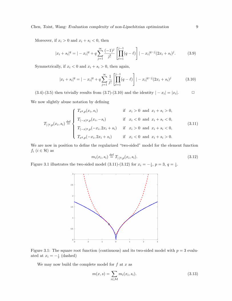
We are now in position to define the regularized “two-sided” model for the element functionfi (i ∈ H) as
mi(xi, si)def= T|·|q ,p(xi, si). (3.12)
Figure 3.1 illustrates the two-sided model (3.11)-(3.12) for xi = − 12, p = 3, q = 1
2.
-3 -2 -1 0 1 2 30
0.5
1
1.5
2
2.5
3
Figure 3.1: The square root function (continuous) and its two-sided model with p = 3 evalu-ated at xi = − 1
2(dashed)
We may now build the complete model for f at x as
m(x, s) =∑i∈M
mi(xi, si). (3.13)
Chen, Toint, Wang: Evaluation complexity of non-Lipschitzian optimization 10
The algorithm considered in this paper exploits the model (3.13) as follows. At eachiteration k, the model (3.13) taken at the iterate x = xk is (approximately) minimized inorder to define a step sk. If the decrease in the objective function value along sk is comparableto that predicted by the Taylor model, the trial point xk + sk is accepted as the new iterateand the regularization parameters σi,k (i.e. σi at iteration k) possibly updated. The processis terminated when an approximate local minimizer is found, that is when, for some k ≥ 0,
χf (xk, ε) ≤ ε. (3.14)
In order to simplify notation in what follows, we make the following definitions:
Ckdef= C(xk, ε), Rk
def= R(xk, ε), Wk
def= W(xk, ε),
andC+k
def= C(xk + sk, ε), R+
kdef= R(xk + sk, ε), W+
kdef= W(xk + sk, ε).
Having defined the criticality measure (2.3), it is natural to use this measure also forterminating the approximate model minimization: to find sk, we therefore minimize m(xk, s)over s until, for some constant θ ≥ 0 and some exponent r > 1,
χm(xk, sk, ε) = χmW+k
(xk, sk, ε) ≤ min
[14q2 min
i∈H∩W+k
|Ui(xk + sk)|r, θ‖sk‖p]
(3.15)
where
χmW+k
(xk, sk, ε)def=
∣∣∣∣∣∣∣∣ minxk+sk+d∈Fd∈R+
k ,‖d‖≤1
∇1smW+
k(xk, sk)
Td
∣∣∣∣∣∣∣∣ . (3.16)
We also require that, once |Ui(xk + s)| < ε occurs for some i ∈ H in the course of themodel minimization, it is fixed at this value, meaning that the remaining minimization iscarried out in R(xk + s, ε). Thus the dimension of R(xk + s, ε) (and therefore of R(xk, ε)) ismonotonically non-increasing during the step computation and across iterations. Note thatcomputing a step sk satisfying (3.15) is always possible since the subspace R(xk + s, ε) canonly become smaller during the model minimization and since we have seen in Section 2 thatχm(xk, sk) = 0 at any local minimizer of mW(xk+s,ε)(xk, s).
3.1 The algorithm
We now introduce some notation useful for describing our algorithm. Define
xi,kdef= Uixk, si,k
def= Uisk.
Also letδfi,k
def= fi(xi,k)− fi(xi,k + si,k)
δfkdef= fW+
k(xk)− fW+
k(xk + sk) =
∑i∈W+
k
δfi,k,
δmi,kdef= mi(xi,k, 0)−mi(xi,k, si,k),
Chen, Toint, Wang: Evaluation complexity of non-Lipschitzian optimization 11
δmkdef= mW+
k(xk, 0)−mW+
k(xk, sk) =
∑i∈W+
k
δmi,k,
and
δTkdef= TfW+
k,p(xk, 0)− TfW+
k,p(xk, sk)
= [TfN ,p(xk, 0)− TfN ,p(xk, sk)] + [T|·|H\C+k,p
(xk, 0)− T|·|H\C+k,p
(xk, sk)]
= δmk + 1(p+ 1)!
∑i∈N
σi,k‖si,k‖p+1.
(3.17)
The partially separable adaptive regularization algorithm is now formally stated as Algorith-m 3.1 on the following page.
Note that an x0 ∈ F can always be computed by projecting an infeasible starting pointonto F . The idea of the second and third parts of (3.21) and (3.22) is to identify caseswhere the model mi overestimates the element function fi to an excessive extent, leavingsome space for reducing the regularization and hence allowing longer steps. The requirementthat ρk ≥ η in both (3.21) and (3.22) is intended to prevent a situation where a particularregularization parameter is increased and another decreased at a given unsuccessful iteration,followed by the opposite situation at the next iteration, potentially leading to cycling. Othermore elaborate mechanisms can be designed to achieve the same goal, such as attempting toreduce a given regularization parameter at most a fixed number of times before the occurenceof a successful iteration, but we do not investigate those alternatives in detail here. Theidea of the second and third parts of (3.21) and (3.22) is simply to identify cases where themodel mi overestimates the element function fi to an excessive extent, leaving some spacefor reducing the regularization and hence allowing longer steps.
We note at this stage that the condition sk ∈ Rk implies that
Ck ⊆ C+k and W+k ⊆ Wk.
Note that the above algorithm considerably simplifies in the Lipschitzian case where H =∅, since
fWk(x) = fM(x) = f(x)
for all k ≥ 0 and all x ∈ F = FQ.
4 Evaluation complexity for ’kernel-centered’ fesible sets
We start our worst-case analysis by formalizing our assumptions for problem (1.1).
AS.1 The feasible set F is closed, convex and non-empty.
AS.2 Each element function fi (i ∈ N ) is p times continuously differentiable in anopen set containing F , where p is odd whenever H 6= ∅.
Chen, Toint, Wang: Evaluation complexity of non-Lipschitzian optimization 12
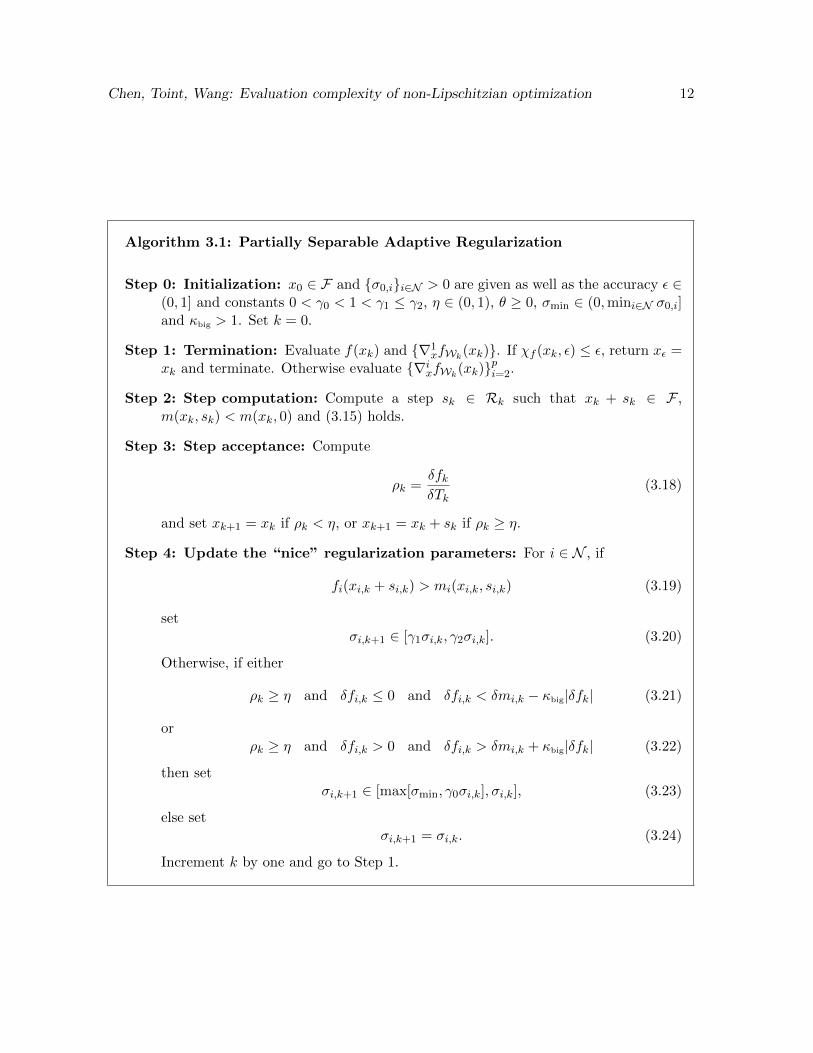
Algorithm 3.1: Partially Separable Adaptive Regularization
Step 0: Initialization: x0 ∈ F and {σ0,i}i∈N > 0 are given as well as the accuracy ε ∈(0, 1] and constants 0 < γ0 < 1 < γ1 ≤ γ2, η ∈ (0, 1), θ ≥ 0, σmin ∈ (0,mini∈N σ0,i]and κbig > 1. Set k = 0.
Step 1: Termination: Evaluate f(xk) and {∇1xfWk
(xk)}. If χf (xk, ε) ≤ ε, return xε =xk and terminate. Otherwise evaluate {∇ixfWk
(xk)}pi=2.
Step 2: Step computation: Compute a step sk ∈ Rk such that xk + sk ∈ F ,m(xk, sk) < m(xk, 0) and (3.15) holds.
Step 3: Step acceptance: Compute
ρk =δfkδTk
(3.18)
and set xk+1 = xk if ρk < η, or xk+1 = xk + sk if ρk ≥ η.
Step 4: Update the “nice” regularization parameters: For i ∈ N , if
fi(xi,k + si,k) > mi(xi,k, si,k) (3.19)
setσi,k+1 ∈ [γ1σi,k, γ2σi,k]. (3.20)
Otherwise, if either
ρk ≥ η and δfi,k ≤ 0 and δfi,k < δmi,k − κbig|δfk| (3.21)
orρk ≥ η and δfi,k > 0 and δfi,k > δmi,k + κbig|δfk| (3.22)
then setσi,k+1 ∈ [max[σmin, γ0σi,k], σi,k], (3.23)
else setσi,k+1 = σi,k. (3.24)
Increment k by one and go to Step 1.
Chen, Toint, Wang: Evaluation complexity of non-Lipschitzian optimization 13
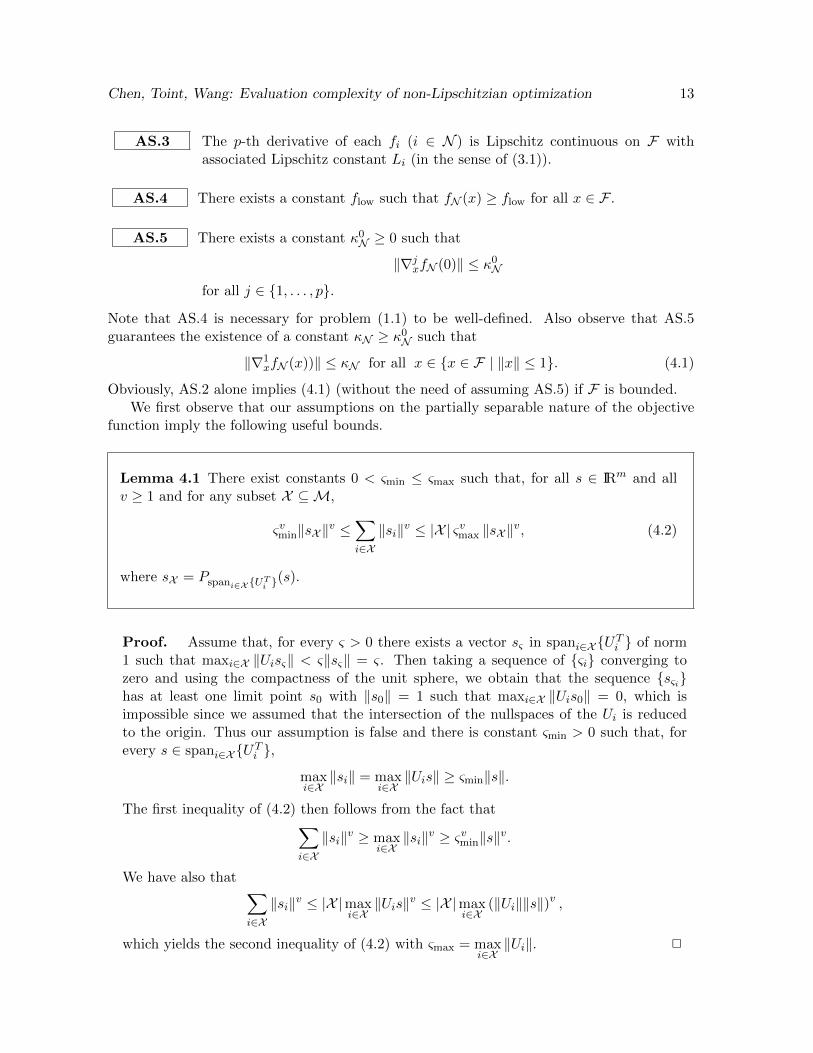
AS.3 The p-th derivative of each fi (i ∈ N ) is Lipschitz continuous on F withassociated Lipschitz constant Li (in the sense of (3.1)).
AS.4 There exists a constant flow such that fN (x) ≥ flow for all x ∈ F .
AS.5 There exists a constant κ0N ≥ 0 such that
‖∇jxfN (0)‖ ≤ κ0Nfor all j ∈ {1, . . . , p}.
Note that AS.4 is necessary for problem (1.1) to be well-defined. Also observe that AS.5guarantees the existence of a constant κN ≥ κ0N such that
‖∇1xfN (x))‖ ≤ κN for all x ∈ {x ∈ F | ‖x‖ ≤ 1}. (4.1)
Obviously, AS.2 alone implies (4.1) (without the need of assuming AS.5) if F is bounded.We first observe that our assumptions on the partially separable nature of the objective
function imply the following useful bounds.
Lemma 4.1 There exist constants 0 < ςmin ≤ ςmax such that, for all s ∈ IRm and allv ≥ 1 and for any subset X ⊆M,
ςvmin‖sX ‖v ≤∑i∈X‖si‖v ≤ |X | ςvmax ‖sX ‖v, (4.2)
where sX = Pspani∈X {UTi }(s).
Proof. Assume that, for every ς > 0 there exists a vector sς in spani∈X {UTi } of norm1 such that maxi∈X ‖Uisς‖ < ς‖sς‖ = ς. Then taking a sequence of {ςi} converging tozero and using the compactness of the unit sphere, we obtain that the sequence {sςi}has at least one limit point s0 with ‖s0‖ = 1 such that maxi∈X ‖Uis0‖ = 0, which isimpossible since we assumed that the intersection of the nullspaces of the Ui is reducedto the origin. Thus our assumption is false and there is constant ςmin > 0 such that, forevery s ∈ spani∈X {UTi },
maxi∈X‖si‖ = max
i∈X‖Uis‖ ≥ ςmin‖s‖.
The first inequality of (4.2) then follows from the fact that∑i∈X‖si‖v ≥ max
i∈X‖si‖v ≥ ςvmin‖s‖v.
We have also that ∑i∈X‖si‖v ≤ |X |max
i∈X‖Uis‖v ≤ |X |max
i∈X(‖Ui‖‖s‖)v ,
which yields the second inequality of (4.2) with ςmax = maxi∈X‖Ui‖. 2
Chen, Toint, Wang: Evaluation complexity of non-Lipschitzian optimization 14
Taken for v = 1 and X = N , this lemma states that∑
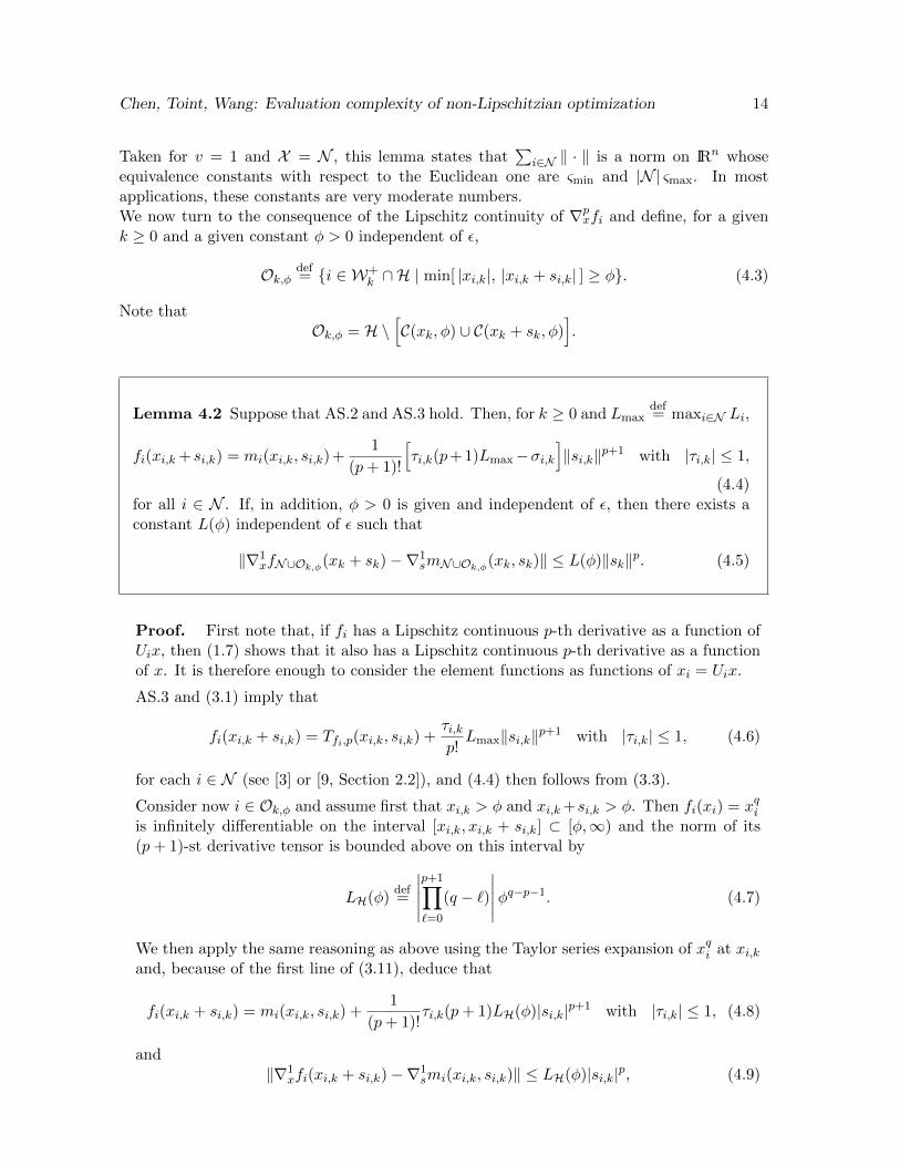
i∈N ‖ · ‖ is a norm on IRn whoseequivalence constants with respect to the Euclidean one are ςmin and |N | ςmax. In mostapplications, these constants are very moderate numbers.We now turn to the consequence of the Lipschitz continuity of ∇pxfi and define, for a givenk ≥ 0 and a given constant φ > 0 independent of ε,
Ok,φdef= {i ∈ W+
k ∩H | min[ |xi,k|, |xi,k + si,k| ] ≥ φ}. (4.3)
Note thatOk,φ = H \
[C(xk, φ) ∪ C(xk + sk, φ)
].
Lemma 4.2 Suppose that AS.2 and AS.3 hold. Then, for k ≥ 0 and Lmaxdef= maxi∈N Li,
fi(xi,k + si,k) = mi(xi,k, si,k) +1
(p+ 1)!
[τi,k(p+ 1)Lmax−σi,k
]‖si,k‖p+1 with |τi,k| ≤ 1,
(4.4)for all i ∈ N . If, in addition, φ > 0 is given and independent of ε, then there exists aconstant L(φ) independent of ε such that
‖∇1xfN∪Ok,φ(xk + sk)−∇1
smN∪Ok,φ(xk, sk)‖ ≤ L(φ)‖sk‖p. (4.5)
Proof. First note that, if fi has a Lipschitz continuous p-th derivative as a function ofUix, then (1.7) shows that it also has a Lipschitz continuous p-th derivative as a functionof x. It is therefore enough to consider the element functions as functions of xi = Uix.
AS.3 and (3.1) imply that
fi(xi,k + si,k) = Tfi,p(xi,k, si,k) +τi,kp!Lmax‖si,k‖p+1 with |τi,k| ≤ 1, (4.6)
for each i ∈ N (see [3] or [9, Section 2.2]), and (4.4) then follows from (3.3).
Consider now i ∈ Ok,φ and assume first that xi,k > φ and xi,k+si,k > φ. Then fi(xi) = xqiis infinitely differentiable on the interval [xi,k, xi,k + si,k] ⊂ [φ,∞) and the norm of its(p+ 1)-st derivative tensor is bounded above on this interval by
LH(φ)def=
∣∣∣∣∣p+1∏`=0
(q − `)
∣∣∣∣∣φq−p−1. (4.7)
We then apply the same reasoning as above using the Taylor series expansion of xqi at xi,kand, because of the first line of (3.11), deduce that
fi(xi,k + si,k) = mi(xi,k, si,k) +1
(p+ 1)!τi,k(p+ 1)LH(φ)|si,k|p+1 with |τi,k| ≤ 1, (4.8)
and‖∇1
xfi(xi,k + si,k)−∇1smi(xi,k, si,k)‖ ≤ LH(φ)|si,k|p, (4.9)
Chen, Toint, Wang: Evaluation complexity of non-Lipschitzian optimization 15
hold in this case (see [3]). The argument is obviously similar if xi,k < −φ and xi,k + si,k <−φ, using symmetry and the second line of (3.11). Let us now consider the case wherexi,k > φ and xi,k + si,k < −φ. The expansion (3.4) then shows that we may reason asfor xi,k < −φ and xi,k + si,k < −φ using a Taylor expansion at −xi (which we know bysymmetry) and the third line of (3.11). The case where xi,k < −φ and xi,k + si,k > φ issimilar, using the fourth line of (3.11). As a consequence, (4.8) and (4.9) hold for everyi ∈ Ok,φ with Lipschitz constant LH(φ). Moreover, using (4.2) and the definitions (4.7),∑
i∈N∪Ok,φ
Li‖si‖p+1 ≤ max [Lmax, LH(φ)]∑
i∈N∪Ok,φ
‖si‖p+1
from which (4.5) may in turn be derived from (4.9) and (4.2) with
L(φ)def= |M| ςp+1
max max [Lmax, LH(φ)] . (4.10)
2
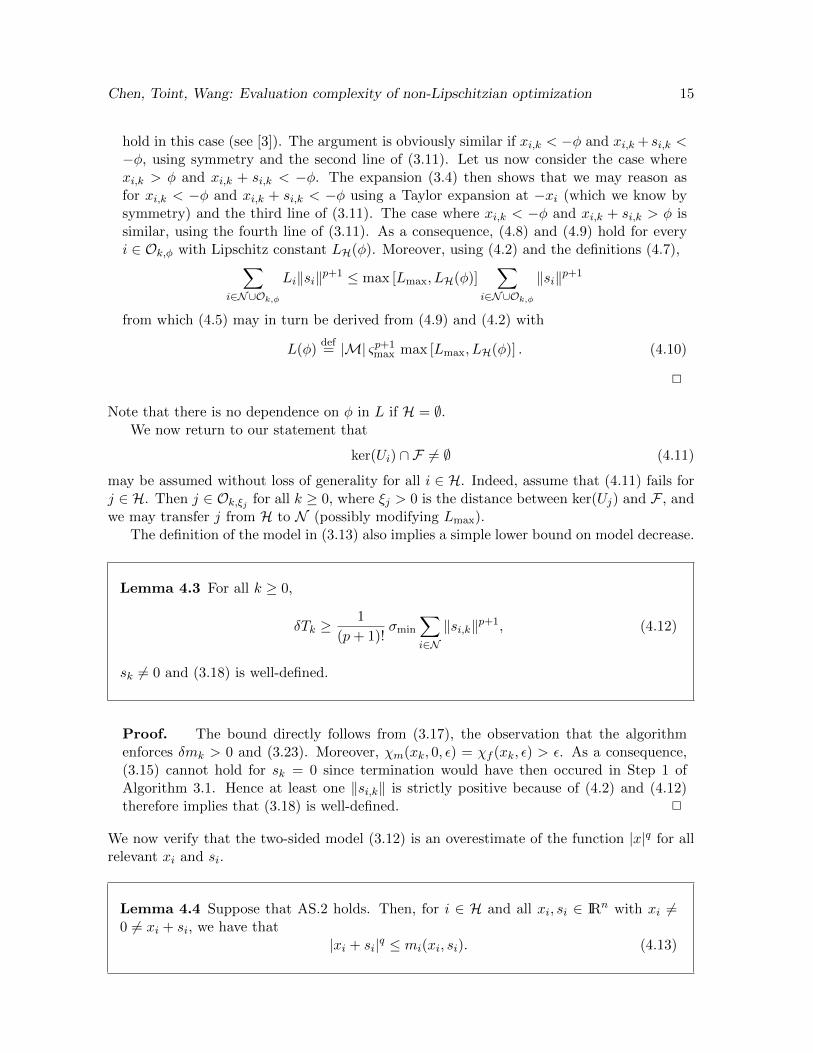
Note that there is no dependence on φ in L if H = ∅.We now return to our statement that
ker(Ui) ∩ F 6= ∅ (4.11)
may be assumed without loss of generality for all i ∈ H. Indeed, assume that (4.11) fails forj ∈ H. Then j ∈ Ok,ξj for all k ≥ 0, where ξj > 0 is the distance between ker(Uj) and F , andwe may transfer j from H to N (possibly modifying Lmax).
The definition of the model in (3.13) also implies a simple lower bound on model decrease.
Lemma 4.3 For all k ≥ 0,
δTk ≥1
(p+ 1)!σmin
∑i∈N‖si,k‖p+1, (4.12)
sk 6= 0 and (3.18) is well-defined.
Proof. The bound directly follows from (3.17), the observation that the algorithmenforces δmk > 0 and (3.23). Moreover, χm(xk, 0, ε) = χf (xk, ε) > ε. As a consequence,(3.15) cannot hold for sk = 0 since termination would have then occured in Step 1 ofAlgorithm 3.1. Hence at least one ‖si,k‖ is strictly positive because of (4.2) and (4.12)therefore implies that (3.18) is well-defined. 2
We now verify that the two-sided model (3.12) is an overestimate of the function |x|q for allrelevant xi and si.
Lemma 4.4 Suppose that AS.2 holds. Then, for i ∈ H and all xi, si ∈ IRn with xi 6=0 6= xi + si, we have that
|xi + si|q ≤ mi(xi, si). (4.13)
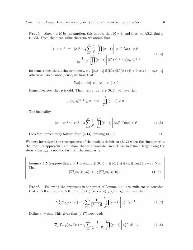
Chen, Toint, Wang: Evaluation complexity of non-Lipschitzian optimization 16
Proof. Since i ∈ H by assumption, this implies that H 6= ∅, and thus, by AS.2, that pis odd. From the mean-value theorem, we obtain that
|xi + si|q = |xi|q + q
p∑j=1
1
j!
[j−1∏`=1
(q − `)
]|xi|q−jµ(xi, si)
j
+ 1(p+ 1)!
[p∏`=1
(q − `)
]|Uiz|q−p−1µ(xi, si)
p+1
(4.14)
for some z such that, using symmetry, z ∈ [x, x+s] if (Uix)(Ui(x+s)) > 0 or z ∈ [−x, x+s]otherwise. As a consequence, we have that
|Uiz| ≥ min[ |xi|, |xi + si| ] > 0.
Remember now that p is odd. Then, using that q ∈ (0, 1), we have that
µ(xi, si)p+1 ≥ 0 and
p∏`=1
(q − `) < 0.
The inequality
|xi + si|q ≤ |xi|q + q
p∑j=1
1
j!
[j−1∏`=1
(q − `)
]|xi|q−jµ(xi, si)
j (4.15)
therefore immediately follows from (4.14), proving (4.13). 2
We next investigate the consequences of the model’s definition (3.12) when the singularity atthe origin is approached and show that the two-sided model has to remain large along thesteps when xi,k is not too far from the singularity.
Lemma 4.5 Suppose that p ≥ 1 is odd, q ∈ (0, 1), i ∈ H, |xi| ∈ (ε, 1], and |xi + si| ≥ ε.Then
|∇1simi(xi, si)| > 1
2q |∇1
simi(xi, 0)|. (4.16)
Proof. Following the argument in the proof of Lemma 4.2, it is sufficient to considerthat xi > 0 and xi + si > 0. From (3.11) (where µ(xi, si) = si), we have that
∇1siTxq ,p(xi, si) = q
p∑j=1
1
(j − 1)!
[j−1∏`=1
(q − `)
]xq−ji sj−1i . (4.17)
Define si = βxi. This gives that (4.17) now reads
∇1siTxq ,p(xi, βxi) = q
p∑j=1
1
(j − 1)!
[j−1∏`=1
(q − `)
]xq−1i βj−1, (4.18)
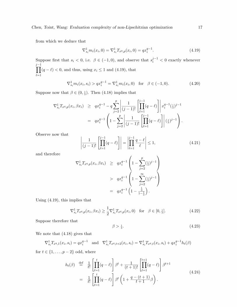
Chen, Toint, Wang: Evaluation complexity of non-Lipschitzian optimization 17
from which we deduce that
∇1simi(xi, 0) = ∇1
siTxq ,p(xi, 0) = qxq−1i . (4.19)
Suppose first that si < 0, i.e. β ∈ (−1, 0), and observe that sj−1i < 0 exactly wheneverj−1∏`=1
(q − `) < 0, and thus, using xi ≤ 1 and (4.19), that
∇1simi(xi, si) > qxq−1i = ∇1
simi(xi, 0) for β ∈ (−1, 0). (4.20)
Suppose now that β ∈ (0, 13). Then (4.18) implies that
∇1siTxq ,p(xi, βxi) ≥ qxq−1i − q
p∑j=2
∣∣∣∣∣ 1
(j − 1)!
[j−1∏`=1
(q − `)
]∣∣∣∣∣xq−1i ( 13)j−1
= qxq−1i
1−p∑j=2
∣∣∣∣∣ 1
(j − 1)!
[j−1∏`=1
(q − `)
]∣∣∣∣∣ ( 13)j−1
.
Observe now that ∣∣∣∣∣ 1
(j − 1)!
[j−1∏`=1
(q − `)
]∣∣∣∣∣ =
∣∣∣∣∣j−1∏`=1
q − ``
∣∣∣∣∣ ≤ 1, (4.21)
and therefore
∇1siTxq ,p(xi, βxi) ≥ qxq−1i
1−p∑j=2
( 13)j−1
> qxq−1i
1−∞∑j=2
( 13)j−1
= qxq−1i
(1−
13
1− 13
).
Using (4.19), this implies that
∇1siTxq ,p(xi, βxi) ≥
1
2∇1siTxq ,p(xi, 0) for β ∈ [0, 1
3]. (4.22)
Suppose therefore thatβ > 1
3. (4.23)
We note that (4.18) gives that
∇1siTxq ,1(xi, si) = qxq−1i and ∇1
siTxq ,t+2(xi, si) = ∇1siTxq ,t(xi, si) + qxq−1i ht(β)
for t ∈ {1, . . . , p− 2} odd, where
ht(β)def= 1
t!
[t∏
`=1
(q − `)
]βt + 1
(t+ 1)!
[t+1∏`=1
(q − `)
]βt+1
= 1t!
[t∏
`=1
(q − `)
]βt(
1 +q − (t+ 1)t+ 1 β
).
(4.24)
Chen, Toint, Wang: Evaluation complexity of non-Lipschitzian optimization 18
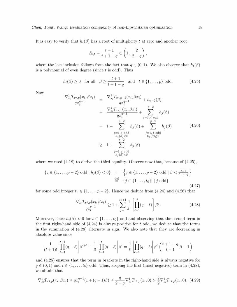
It is easy to verify that ht(β) has a root of multiplicity t at zero and another root
β0,t =t+ 1
t+ 1− q∈(
1 ,2
2− q
),
where the last inclusion follows from the fact that q ∈ (0, 1). We also observe that ht(β)is a polynomial of even degree (since t is odd). Thus
ht(β) ≥ 0 for all β ≥ t+ 1
t+ 1− qand t ∈ {1, . . . , p} odd. (4.25)
Now∇1siTxq ,p(xi, βxi)
qxq−1i
=∇1siTxq ,p−2(xi, βxi)
qxq−1i
+ hp−2(β)
=∇1siTxq ,1(xi, βxi)
qxq−1i
+
p−2∑j=1, j odd
hj(β)
= 1 +
p−2∑j=1, j oddhj(β)<0
hj(β) +
p−2∑j=1, j oddhj(β)≥0
hj(β)
≥ 1 +
p−2∑j=1, j oddhj(β)<0
hj(β)
(4.26)
where we used (4.18) to derive the third equality. Observe now that, because of (4.25),
{j ∈ {1, . . . , p− 2} odd | hj(β) < 0} ={j ∈ {1, . . . , p− 2} odd | β < t+1
t+1−q
}def= {j ∈ {1, . . . , t0}| | j odd}
(4.27)for some odd integer t0 ∈ {1, . . . , p− 2}. Hence we deduce from (4.24) and (4.26) that
∇1siTxq ,p(xi, βxi)
qxq−1i
≥ 1 +
t0+1∑j=1
1
j!
[j∏`=1
(q − `)
]βj . (4.28)
Moreover, since ht(β) < 0 for t ∈ {1, . . . , t0} odd and observing that the second term inthe first right-hand side of (4.24) is always positive for t odd, we deduce that the termsin the summation of (4.28) alternate in sign. We also note that they are decreasing inabsolute value since
1
(t+ 1)!
∣∣∣∣∣t+1∏`=1
(q − `)
∣∣∣∣∣βt+1 − 1
t!
∣∣∣∣∣t∏
`=1
(q − `)
∣∣∣∣∣βt =1
t!
∣∣∣∣∣t∏
`=1
(q − `)
∣∣∣∣∣βt(t+ 1− qt+ 1
β − 1
)and (4.25) ensures that the term in brackets in the right-hand side is always negative forq ∈ (0, 1) and t ∈ {1, . . . , t0} odd. Thus, keeping the first (most negative) term in (4.28),we obtain that
∇1siTxq ,p(xi, βxi) ≥ qx
q−1i (1 + (q− 1)β) ≥ q
2− q∇1siTxq ,p(xi, 0) >
q
2∇1siTxq ,p(xi, 0). (4.29)
Chen, Toint, Wang: Evaluation complexity of non-Lipschitzian optimization 19
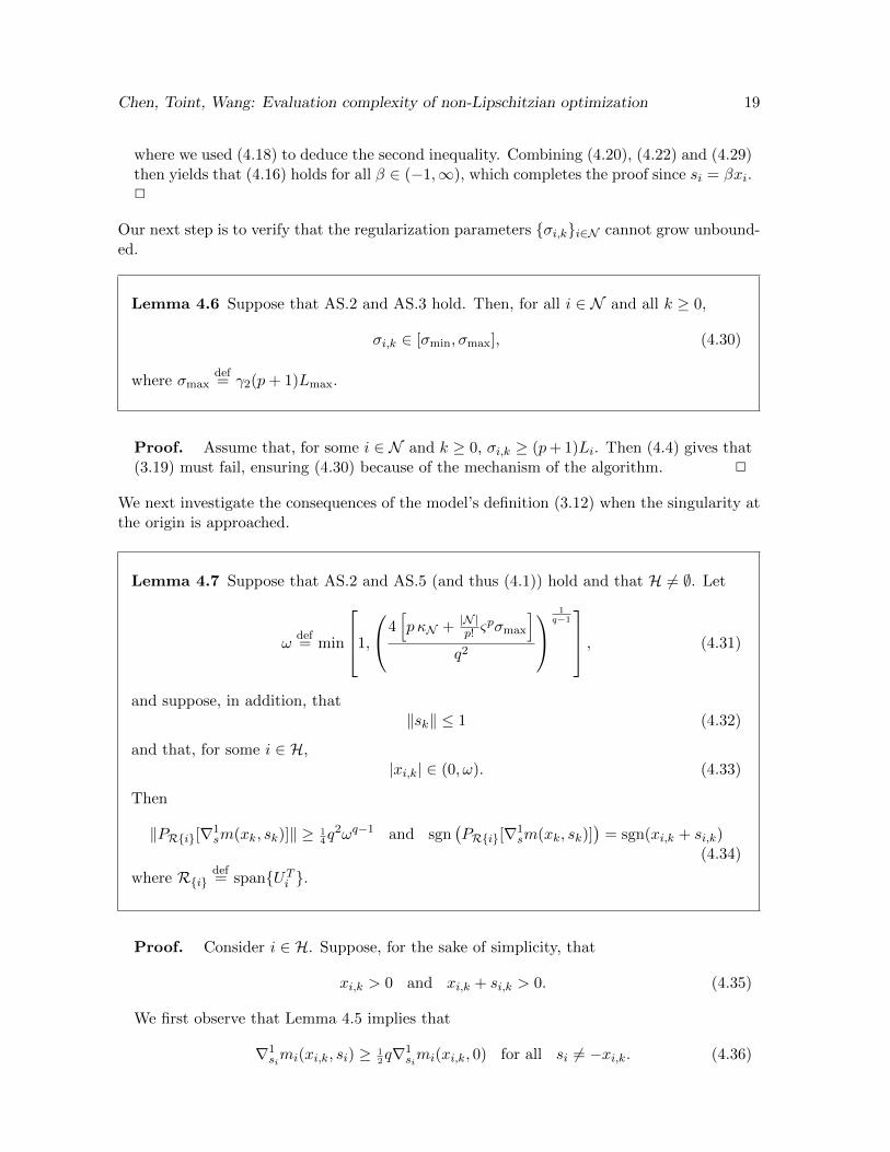
where we used (4.18) to deduce the second inequality. Combining (4.20), (4.22) and (4.29)then yields that (4.16) holds for all β ∈ (−1,∞), which completes the proof since si = βxi.2
Our next step is to verify that the regularization parameters {σi,k}i∈N cannot grow unbound-ed.
Lemma 4.6 Suppose that AS.2 and AS.3 hold. Then, for all i ∈ N and all k ≥ 0,
σi,k ∈ [σmin, σmax], (4.30)
where σmaxdef= γ2(p+ 1)Lmax.
Proof. Assume that, for some i ∈ N and k ≥ 0, σi,k ≥ (p+ 1)Li. Then (4.4) gives that(3.19) must fail, ensuring (4.30) because of the mechanism of the algorithm. 2
We next investigate the consequences of the model’s definition (3.12) when the singularity atthe origin is approached.
Lemma 4.7 Suppose that AS.2 and AS.5 (and thus (4.1)) hold and that H 6= ∅. Let
ωdef= min
1,
4[p κN + |N |
p! ςpσmax
]q2
1q−1
, (4.31)
and suppose, in addition, that‖sk‖ ≤ 1 (4.32)
and that, for some i ∈ H,|xi,k| ∈ (0, ω). (4.33)
Then
‖PR{i}[∇1sm(xk, sk)]‖ ≥ 1
4q2ωq−1 and sgn
(PR{i}[∇1
sm(xk, sk)])
= sgn(xi,k + si,k)(4.34)
where R{i}def= span{UTi }.
Proof. Consider i ∈ H. Suppose, for the sake of simplicity, that
xi,k > 0 and xi,k + si,k > 0. (4.35)
We first observe that Lemma 4.5 implies that
∇1simi(xi,k, si) ≥ 1
2q∇1
simi(xi,k, 0) for all si 6= −xi,k. (4.36)
Chen, Toint, Wang: Evaluation complexity of non-Lipschitzian optimization 20
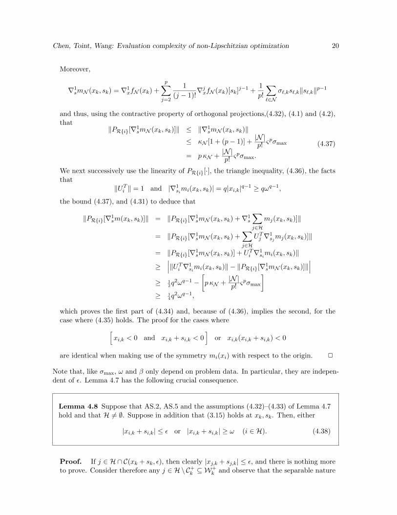
Moreover,
∇1smN (xk, sk) = ∇1
xfN (xk) +
p∑j=2
1
(j − 1)!∇jxfN (xk)[sk]
j−1 +1
p!
∑`∈N
σ`,ks`,k‖s`,k‖p−1
and thus, using the contractive property of orthogonal projections,(4.32), (4.1) and (4.2),that
‖PR{i}[∇1smN (xk, sk)]‖ ≤ ‖∇1
smN (xk, sk)‖≤ κN [1 + (p− 1)] +
|N |p!ςpσmax
= p κN +|N |p!ςpσmax.
(4.37)
We next successively use the linearity of PR{i}[·], the triangle inequality, (4.36), the factsthat
‖UTi ‖ = 1 and |∇1simi(xk, sk)| = q|xi,k|q−1 ≥ qωq−1,
the bound (4.37), and (4.31) to deduce that
‖PR{i}[∇1sm(xk, sk)]‖ = ‖PR{i}[∇1
smN (xk, sk) +∇1s
∑j∈H
mj(xk, sk)]‖
= ‖PR{i}[∇1smN (xk, sk) +
∑j∈H
UTj ∇1sjmj(xk, sk)]‖
= ‖PR{i}[∇1smN (xk, sk)] + UTi ∇1
simi(xk, sk)‖
≥∣∣∣‖UTi ∇1
simi(xk, sk)‖ − ‖PR{i}[∇1smN (xk, sk)]‖
∣∣∣≥ 1
2q2ωq−1 −
[p κN +
|N |p!ςpσmax
]≥ 1
4q2ωq−1,
which proves the first part of (4.34) and, because of (4.36), implies the second, for thecase where (4.35) holds. The proof for the cases where[
xi,k < 0 and xi,k + si,k < 0]
or xi,k(xi,k + si,k) < 0
are identical when making use of the symmetry mi(xi) with respect to the origin. 2
Note that, like σmax, ω and β only depend on problem data. In particular, they are indepen-dent of ε. Lemma 4.7 has the following crucial consequence.
Lemma 4.8 Suppose that AS.2, AS.5 and the assumptions (4.32)–(4.33) of Lemma 4.7hold and that H 6= ∅. Suppose in addition that (3.15) holds at xk, sk. Then, either
|xi,k + si,k| ≤ ε or |xi,k + si,k| ≥ ω (i ∈ H). (4.38)
Proof. If j ∈ H ∩ C(xk + sk, ε), then clearly |xj,k + sj,k| ≤ ε, and there is nothing moreto prove. Consider therefore any j ∈ H\C+k ⊆ W
+k and observe that the separable nature
Chen, Toint, Wang: Evaluation complexity of non-Lipschitzian optimization 21
of the linear optimization problem in (3.16) implies that∣∣∣∣∣∣∣ minxk+sk+d∈Fd∈R{j},‖d‖≤1
PR{j} [∇1sm(xk, sk)]
Td
∣∣∣∣∣∣∣ =
∣∣∣∣∣∣∣ minxk+sk+d∈Fd∈R{j},‖d‖≤1
∇1smW+
k(xk, sk)
Td
∣∣∣∣∣∣∣≤
∣∣∣∣∣∣∣∣ minxk+sk+d∈Fd∈R+
k ,‖d‖≤1
∇1smW+
k(xk, sk)
Td
∣∣∣∣∣∣∣∣= χm(xk, sk, ε)
≤ 14q2|xj,k + sj,k|r.
(4.39)
Observe now that, because of the second part of (4.34) and the fact that nj = 1 becauseof (1.2), the optimal value for the convex optimization problem in the left-hand side ofthis relation is given by
|PR{j} [∇1sm(xk, sk)]| |d∗|
where d∗ is the problem solution and d∗ has the opposite sign of PR{j} [∇1sm(xk, sk)].
Moreover, the facts that j ∈ H and (1.3) ensure that xj,k + sj,k + dj = 0 is feasible for theoptimization problem on the left-hand side of (4.39), and hence that |d∗| ≥ |xj,k + sj,k|.Hence, we obtain that
14q2ωq−1|xj,k + sj,k| ≤ 1
4q2|xj,k + sj,k|r,
and thus, since ω ≤ 1, that
|xj,k + sj,k| ≥ ωq−1r−1 ≥ ω,
and the second alternative in (4.38) holds. 2
The rest of our complexity analysis depends on the following partitioning of the set of itera-tions. Let the index set of the “successful” and “unsuccessful” iterations be given by
S def= {k ≥ 0 | ρk ≥ η} and U def
= {k ≥ 0 | ρk < η}.
We next focus on the case where H 6= ∅ and partition S into subsets depending on |xi,k| and|xi,k + si,k| for i ∈ H. We first isolate the set of sucessful iterations which “deactivate” somevariable, that is
Sεdef= {k ∈ S | |xi,k + si,k| ≤ ε for some i ∈ H},
as well as the set of successful iterations with large steps
S‖s‖def= {k ∈ S \ Sε | ‖sk‖ > 1}. (4.40)
Let us now choose a constant α ≥ 0 such that
α =
{34ω if H 6= ∅,
0 otherwise.(4.41)
Chen, Toint, Wang: Evaluation complexity of non-Lipschitzian optimization 22
Then, at iteration k ∈ S \ (Sε ∪ S‖s‖), we distinguish
I♥,kdef={i ∈ H \ Ck | |xi,k| ∈ [α,+∞) and |xi,k + si,k| ∈ [α,+∞)
},
I♦,kdef={i ∈ H \ Ck |
(|xi,k| ∈ [ω,+∞) and |xi,k + si,k| ∈ (ε, α)
)or(|xi,k| ∈ (ε, α) and |xi,k + si,k| ∈ [ω,+∞)
)},
I♣,kdef={i ∈ H \ Ck | |xi,k| ∈ (ε, ω) and |xi,k + si,k| ∈ (ε, ω)
}.
Using these notations, we further define
S♥def= {k ∈ S \ (Sε ∪ S‖s‖) | I♥,k = H \ Ck}, S♦
def= {k ∈ S \ (Sε ∪ S‖s‖) | I♦,k 6= ∅},
S♣def= {k ∈ S \ (Sε ∪ S‖s‖) | I♣,k 6= ∅}.
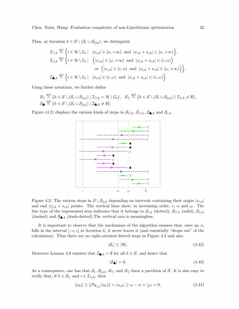
Figure (4.2) displays the various kinds of steps in S♥,k, S♦,k, S♣,k and Sε,k.
ε α ω 1
♥
♥
♥
♦
♣
♣
ε
♣
ε
♣
♣
ε
♦
♥
♥
Figure 4.2: The various steps in S \ S‖s‖ depending on intervals containing their origin |xi,k|and end |xi,k + si,k| points. The vertical lines show, in increasing order, ε, α and ω. Theline type of the represented step indicates that it belongs to Sε,k (dotted), S♥,k (solid), S♦,k(dashed) and S♣,k (dash-dotted).The vertical axis is meaningless.
It is important to observe that the mechanism of the algorithm ensures that, once an xifalls in the interval [−ε, ε] at iteration k, it never leaves it (and essentially “drops out” of thecalculation). Thus there are no right-oriented dotted steps in Figure 4.2 and also
|Sε| ≤ |H|. (4.42)
Moreover Lemma 4.8 ensures that I♣,k = ∅ for all k ∈ S, and hence that
|S♣| = 0. (4.43)
As a consequence, one has that Sε, S‖s‖, S♥, and S♦ form a partition of S. It is also easy toverify that, if k ∈ S♦ and i ∈ I♦,k, then
‖sk‖ ≥ ‖PR{i}(sk)‖ = |si,k| ≥ ω − α = 14ω > 0, (4.44)
Chen, Toint, Wang: Evaluation complexity of non-Lipschitzian optimization 23
where we have used the contractive property of orthogonal projections.We now show that the steps at iterations whose index is in S♥ are not too short.
Lemma 4.9 Suppose that AS.1-AS.3 and AS.5 hold, that
ε < α (4.45)
and consider k ∈ S♥ before termination. Then
‖sk‖ ≥ (κ♥ ε)1p , (4.46)
where
κ♥def=
[2(L(α) + θ +
|N |p!
ςp+1max σmax)
]−1. (4.47)
Proof. Observe first that, since k ∈ S♥ ⊆ S, we have that xk+1 = xk + sk and, becauseε ≤ α and C+k ⊆ Ck, we deduce that Ck = C+k = Ck+1 and Rk = R+
k = Rk+1. Moreoverthe definition of S♥ ensures that, for all i ∈ H \ Ck,
min[|xi,k|, |xi,k + si,k|
]≥ α. (4.48)
HenceO∗
def= Ok,α = H \ Ck = H \ C+k ,
and thusR∗
def= Rk = R+
k and W∗def= Wk =W+
k = N ∪O∗. (4.49)
As a consequence the step computation must have been completed because (3.15) holds,which implies that
χm(xk, sk, ε) = χmW∗ (xk, sk, ε) =
∣∣∣∣∣∣∣ minxk+sk+d∈Fd∈R∗,‖d‖≤1
∇smW∗(xk, sk)Td
∣∣∣∣∣∣∣ ≤ θ‖sk‖p. (4.50)
Observe also that (4.49), (4.5) with φ = α (because k ∈ S♥) , (4.30) and (4.2) then implythat
‖∇1xfW∗(xk+1)−∇1
smW∗(xk, sk)‖ = ‖∇1xfN∪O∗(xk+1)−∇1
smN∪O∗(xk, sk)‖
≤ L(α)‖sk‖p + 1(p+ 1)!
σmax
∑i∈N‖∇1
s‖si,k‖p+1 ‖
≤ L(α)‖sk‖p + 1p!σmax
∑i∈N‖si,k‖p
≤ L(α)‖sk‖p +|N |p!
ςp+1max σmax‖sk‖p
=
[L(α) +
|N |p!
ςp+1max σmax
]‖sk‖p,
(4.51)
Chen, Toint, Wang: Evaluation complexity of non-Lipschitzian optimization 24
and also that
χf (xk+1, ε) = |∇1xfW∗(xk+1)[dk+1]|
≤ |∇1xfW∗(xk+1)[dk+1]−∇1
smW∗(xk, sk)[dk+1]|+|∇1
smW∗(xk, sk)[dk+1]|,(4.52)
where the first equality defines the vector dk+1 with
‖dk+1‖ ≤ 1. (4.53)
Assume now, for the purpose of deriving a contradiction, that
‖sk‖ <
χf (xk+1, ε)
2(L(α) + θ +|N |p!
ςp+1max σmax)
1p
(4.54)
at iteration k ∈ S♥. Using (4.53) and (4.51), we then obtain that
−∇1xfW∗(xk+1)[dk+1] +∇1
smW∗(xk, sk)[dk+1]
≤ |∇1xfW∗(xk+1)[dk+1]−∇1
smW∗(xk, sk)[dk+1]|
= |(∇1xfW∗(xk+1)−∇1
smW∗(xk, sk))[dk+1]|
≤ ‖∇1xfW∗(xk+1)−∇1
smW∗(xk, sk)‖ ‖dk+1‖
< (L(α) +|N |p!
ςp+1max σmax)‖sk‖p.
(4.55)
From (4.54) and the first part of (4.52), we have that
−∇1xfW∗(xk+1)[dk+1] +∇1
smW∗(xk, sk))[dk+1] < 12χf (xk+1, ε)
= − 12∇1xfW∗(xk+1)[dk+1],
which in turn ensures that
∇1smW∗(xk, sk)[dk+1] < 1
2∇1xfW∗(xk+1)[dk+1] < 0.
Moreover, by definition of χf (xk+1, ε),
xk+1 + dk+1 ∈ F and dk+1 ∈ Rk+1 = R+k .
Hence, using (3.16) and (4.53),
|∇1smW∗(xk, sk)[dk+1]| ≤ χmW∗ (xk, sk, ε). (4.56)
We may then substitute this inequality in (4.52) to deduce as above that
χf (xk+1) ≤ |∇1xfW∗(xk+1)[dk+1]−∇1
smW∗(xk, sk)[dk+1]|+ χmW∗ (xk, sk, ε)
≤ (L(α) + θ +|N |p!
ςp+1max σmax)‖sk‖p
(4.57)
where the last inequality results from (4.55), the identity xk+1 = xk + sk and (4.50). Butthis contradicts our assumption that (4.54) holds. Hence (4.54) must fail. The inequality(4.46) then follows by combining this conclusion with the fact that χf (xk+1, ε) > ε beforetermination. 2
Chen, Toint, Wang: Evaluation complexity of non-Lipschitzian optimization 25
We are now ready to consider our first complexity result, whose proof uses restrictions of thesuccessful and unsuccessful iteration index sets defined above to {0, . . . , k}, which are givenby
Skdef= {0, . . . , k} ∩ S, Uk
def= {0, . . . , k} \ Sk, (4.58)
respectively.
Theorem 4.10 Suppose that AS.1-AS.5 hold and that
ε ≤[α,
(14ωκ− 1p+1
♥
)p]if H 6= ∅. (4.59)
Then Algorithm 3.1 requires at most
κS(f(x0)− flow)ε− p+1
p + |H| (4.60)
successful iterations to return a point xε ∈ F such that χf (xε, ε) ≤ ε, for
κS =(p+ 1)!
η σmin ςp+1min
[2(L(α) + θ +
|N |p!
ςp+1max γ2)
] p+1p. (4.61)
Proof. Let k ∈ S be index of a successful iteration before termination, and suppose firstthat H 6= ∅. Because the iteration is successful, we obtain, using AS.4 and Lemma 4.3,that
f(x0)− flow ≥ f(x0)− f(xk+1) ≥∑`∈Sk
[f(x`)− f(x` + s`)
]≥ η
∑`∈Sk
[f(x`)− Tf,p(x`, s`)
].
(4.62)In addition to (4.58), let us define
Sε,kdef= {0, . . . , k} ∩ Sε, S‖s‖,k
def= {0, . . . , k} ∩ S‖s‖, (4.63)
S♥,kdef= {0, . . . , k} ∩ S♥, S♦,k
def= {0, . . . , k} ∩ S♦.
Chen, Toint, Wang: Evaluation complexity of non-Lipschitzian optimization 26
We now use the fact that S‖s‖,k ∪ S♥,k ∪ S♦,k = Sk \ Sε,k ⊆ Sk, and (4.2) to deduce from(4.62) that
f(x0)− flow ≥ η
∑`∈S‖s‖,k
[f(x`)− Tf,p(x`, s`)
]+∑
`∈S♥,k
[f(x`)− Tf,p(x`, s`)
]
+∑
`∈S♦,k
[f(x`)− Tf,p(x`, s`)
]≥ ησmin
(p+ 1)!
{|S‖s‖,k| min
`∈S‖s‖,k
[∑i∈N‖si,`‖p+1
]+ |S♥,k| min
`∈S♥,k
[∑i∈N‖si,`‖p+1
]
+ |S♦,k| min`∈S♦,k
[∑i∈N‖si,`‖p+1
]}
≥ ησminςp+1min
(p+ 1)!
{|S‖s‖,k| min
`∈S‖s‖,k‖s`‖p+1 + |S♥,k| min
`∈S♥,k‖s`‖p+1
+ |S♦,k| min`∈S♦,k
‖s`‖p+1
}.
Because of of (4.40), (4.63), Lemma 4.9 and (4.44), this now yields that
f(x0)− flow ≥ ησminςp+1min
(p+ 1)!
{|S‖s‖,k|+ |S♥,k|(κ♥ε)
p+1p + |S♦|,k(ω − α)p+1
}≥ ησminς
p+1min
(p+ 1)!
{|S‖s‖,k|+ |S♥,k|+ |S♦,k|
}min
[(κ♥ε)
p+1p , ( 1
4ω)p+1
]≥ ησminς
p+1min
(p+ 1)!|Sk \ Sε| (κ♥ε)
p+1p
where we used (4.59), the partition of Sk \ Sε,k in S‖s‖,k ∪ S♥,k ∪ S♦,k and the inequality14ω < 1 to obtain the last inequality. Thus
|Sk| ≤ κS(f(x0)− flow)ε− p+1
p + |Sε,k|, (4.64)
where κS is given by (4.61). The desired iteration complexity (4.60) then follows fromthis bound, |Sε,k| ≤ |Sε| and (4.42). 2
To complete our analysis in terms of evaluations rather than successful iterations, we need tobound the total number of all (successful and unsuccessful) iterations.
Lemma 4.11 Assume that AS.2 and AS.3 hold. Then, for all k ≥ 0,
k ≤ κa|Sk|+ κb,
where
κadef= 1 +
|N | | log γ0|log γ1
and κbdef=|N |
log γ1log
(σmax
σmin
).
Chen, Toint, Wang: Evaluation complexity of non-Lipschitzian optimization 27
Proof. For i ∈ N , define
Ji,kdef= {j ∈ {0, . . . , k} | (3.20) holds with k ← j},
(the set of iterations where σi,j is increased) and
Di,kdef= {j ∈ {0, . . . , k} | (3.23) holds with k ← j} ⊆ Sk
(the set of iterations where σi,j in decreased), the final inclusion resulting from the con-dition that ρk ≥ η in both (3.21) and (3.22). Observe also that the mechanism of thealgorithm, the fact that γ0 ∈ (0, 1) and Lemma 4.6 impose that, for each i ∈ N ,
σminγ|Ji,k|1 γ
|Sk|0 ≤ σi,0γ
|Ji,k|1 γ
|Di,k|0 ≤ σi,k ≤ σmax.
Dividing by σmin > 0 and taking logarithms yields that, for all i ∈ N and all k > 0,
|Ji,k| log γ1 + |Sk| log γ0 ≤ log
(σmax
σmin
). (4.65)
Note now that, if (3.19) fails for all i ∈ N and given that Lemma 4.4 ensures thatfi(xi + si) ≤ mi(xi, si) for i ∈ H \ C+k , then
δfk =∑i∈W+
k
δfi,k ≥∑i∈W+
k
δmi,k = δmk.
Thus, in view of (3.18), we have that ρk ≥ 1 > η and iteration k is successful. Thus, ifiteration k is unsuccessful, σi,k is increased with (3.20) for at least one i ∈ N . Hence wededuce that
|Uk| ≤∑i∈N|Ji,k| ≤ |N | max
i∈N|Ji,k|. (4.66)
The desired bound follows from (4.65) and (4.66) by using the fact that k = |Sk|+|Uk|−1 ≤|Sk|+ |Uk|, the term -1 in the equality accounting for iteration 0. 2
We may now state our main evaluation complexity result.
Theorem 4.12 Suppose that AS.1, (1.3), AS.2-AS.5 and (4.59) hold. Then Algorith-m 3.1 using models (3.12) for i ∈ H requires at most
κa[κS(f(x0)− flow)ε
− p+1p + |H|
]+ κb + 1 (4.67)
iterations and evaluations of f and its first p derivatives to return a point xε ∈ F suchthat χf (xε, ε) ≤ ε.
Proof. If termination occurs at iteration 0, the theorem obviously holds. Assumetherefore that termination occurs at iteration k + 1, in which case there must be at leastone successful iteration. We may therefore deduce the desired bound from Theorem 4.10,
Chen, Toint, Wang: Evaluation complexity of non-Lipschitzian optimization 28
Lemma 4.11 and the fact that each successful iteration involves the evaluation of f(xk)and {∇ixfWk
(xk)}pi=1, while each unsuccessful iteration only involves that of f(xk) and∇1xfWk
(xk). 2
Note that we may count derivatives’ evaluations in Theorem 4.12 because only the deriva-tives of fWk
are ever evaluated, and these are well-defined. For completeness, we state thecomplexity bound of the important purely Lipschitzian case.
Corollary 4.13 Suppose that AS.1-AS.4 hold and H = ∅. Then Algorithm 3.1 requiresat most
κa[κS(f(x0)− flow)ε
− p+1p
]+ κb + 1
iterations and evaluations of f and its first p derivatives to return a point xε ∈ F suchthat
χf (xε)def=
∣∣∣∣∣∣∣ minx+d∈F‖d‖≤1
∇1xfW(x)(x)Td
∣∣∣∣∣∣∣ ≤ ε.
Proof. Directly follows from Theorem 4.12, H = ∅ and the obesrvation that R(x, ε) =IRn for all x ∈ F since C(x, ε) = ∅. 2
5 Evaluation complexity for general convex FThe two-sided model (3.12) has clear advantages, the main ones being that, except at theorigin where it is non-smooth, it is polynomial and has finite gradients (and higher derivatives)over each of its two branches. It is not however without drawbacks. The first of these is thatits prediction for the gradient (and higher derivatives) is arbitrarily inaccurate as the originis approached, the second being its evaluation cost which is typically higher than evaluating|x+s|q or its derivative directly. In particular, it is the first drawback that required the carefulanalysis of Lemma 4.5, in turn leading, via Lemma 4.7, to the crucial Lemma 4.8. This issignificant because this last lemma, in addition to the use of (3.12) and the requirement thatp must be odd, also requires the ’kernel-centered’ assumption (1.3), a sometimes undesirablerestriction of the feasible domain geometry.
In the case where evaluating fN is very expensive and the convex F is not ’kernel-centered’,it may sometimes be acceptable to push the difficulty of handling the non-Lipschitzian natureof the `q norm regularization in the subproblem of computing sk, if evaluations of fN can besaved. In this context, a simple alternative is then to use
mi(xi, si) = |xi + si|q for i ∈ H (5.1)
that is mi(xi, si) = fi(xi + si) for i ∈ H. The cost of finding a suitable step satisfying(3.15) may of course be increased, but, as we already noted, this cost is irrelevant for worst-case evaluation analysis as long as only the evaluation of fN and its derivatives is takeninto account. The choice (5.1) clearly maintains the overestimation property of Lemma 4.4.
Chen, Toint, Wang: Evaluation complexity of non-Lipschitzian optimization 29
Moreover, it is easy to verify (using AS.3 and (5.1)) that
‖∇xfW+k
(xk+sk)−∇1smW+
k(xk, sk)‖ = ‖∇xfN (xk+sk)−∇1
smN (xk, sk)‖ ≤ Lmax‖sk‖p. (5.2)
This in turn implies that the proof of Lemma 4.9 can be extended without requiring (4.48)and using O∗ = H \ C+k . The derivation of (4.51) then simplifies because of (5.2) and holdsfor all i ∈ H \ C+k with L(α) = Lmax, so that (4.46) holds for all k ∈ S, the assumption (4.45)being now irrelevant. This result then implies that the distinction made between S♥, S♦,S♣ and S‖s‖ is unecessary because (4.46) holds for all k ∈ S = S♥. Moreover, since we nolonger need Lemma 4.8 to prove that S♣ = ∅, we no longer need the restrictions that p isodd and (1.3) either. As consequence, we deduce that Theorem 4.10 holds for arbitrary p ≥ 1and for arbitrary convex, closed non-empty F , without the need to assume (4.59) and withL(α) replaced by Lmax in (4.61). Without altering Lemma 4.11, we may therefore deduce thefollowing complexity result.
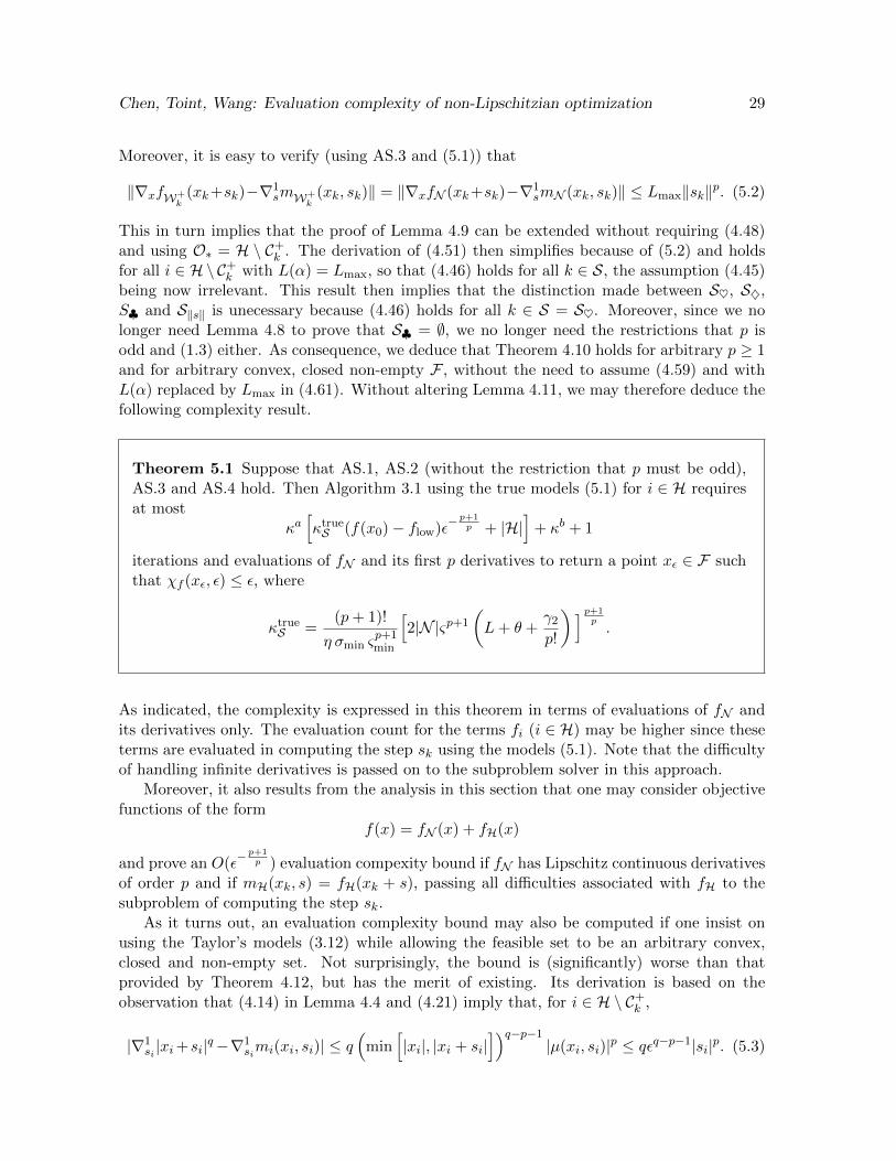
Theorem 5.1 Suppose that AS.1, AS.2 (without the restriction that p must be odd),AS.3 and AS.4 hold. Then Algorithm 3.1 using the true models (5.1) for i ∈ H requiresat most
κa[κtrueS (f(x0)− flow)ε
− p+1p + |H|
]+ κb + 1
iterations and evaluations of fN and its first p derivatives to return a point xε ∈ F suchthat χf (xε, ε) ≤ ε, where
κtrueS =(p+ 1)!
η σmin ςp+1min
[2|N |ςp+1
(L+ θ +
γ2p!
)] p+1p.
As indicated, the complexity is expressed in this theorem in terms of evaluations of fN andits derivatives only. The evaluation count for the terms fi (i ∈ H) may be higher since theseterms are evaluated in computing the step sk using the models (5.1). Note that the difficultyof handling infinite derivatives is passed on to the subproblem solver in this approach.
Moreover, it also results from the analysis in this section that one may consider objectivefunctions of the form
f(x) = fN (x) + fH(x)
and prove an O(ε− p+1
p ) evaluation compexity bound if fN has Lipschitz continuous derivativesof order p and if mH(xk, s) = fH(xk + s), passing all difficulties associated with fH to thesubproblem of computing the step sk.
As it turns out, an evaluation complexity bound may also be computed if one insist onusing the Taylor’s models (3.12) while allowing the feasible set to be an arbitrary convex,closed and non-empty set. Not surprisingly, the bound is (significantly) worse than thatprovided by Theorem 4.12, but has the merit of existing. Its derivation is based on theobservation that (4.14) in Lemma 4.4 and (4.21) imply that, for i ∈ H \ C+k ,
|∇1si |xi+si|q−∇1
simi(xi, si)| ≤ q(
min[|xi|, |xi + si|
])q−p−1|µ(xi, si)|p ≤ qεq−p−1|si|p. (5.3)
Chen, Toint, Wang: Evaluation complexity of non-Lipschitzian optimization 30
This bound can then be used in a variant of Lemma 4.9 just like (5.2) was in Section 5. Inthe updated version of Lemma 4.9, we replace L(α) by
L∗def= |N | ςpmax Lmax + |H| ςpmax q
and (4.51) now becomes
‖∇1xfW+
k(xk+1)−∇1
smW+k
(xk, sk)‖ ≤[L∗ε
q−p−1 +|N |p!ςpσmax
]‖sk‖p.
This results in replacing (4.57) by
χf (xk+1) ≤ (L∗εq−p−1+θ+
|N |p!
ςp+1max σmax)‖sk‖p ≤ (L∗+θ+
|N |p!
ςp+1max σmax)εq−p−1‖sk‖p (5.4)
and therefore (4.46) is replaced by
‖sk‖ ≥[2
(L∗ + θ +
|N |p!
ςp+1max σmax
)]− 1p
εp+2−qp .
We may now follow the steps leading to Theorem 5.1 and deduce a new complexity bound.
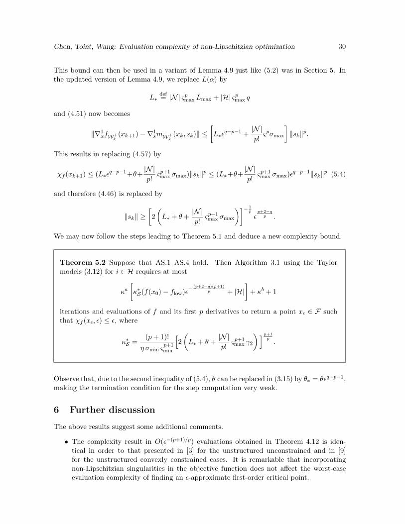
Theorem 5.2 Suppose that AS.1–AS.4 hold. Then Algorithm 3.1 using the Taylormodels (3.12) for i ∈ H requires at most
κa[κ∗S(f(x0)− flow)ε
− (p+2−q)(p+1)p + |H|
]+ κb + 1
iterations and evaluations of f and its first p derivatives to return a point xε ∈ F suchthat χf (xε, ε) ≤ ε, where
κ∗S =(p+ 1)!
η σmin ςp+1min
[2
(L∗ + θ +
|N |p!
ςp+1max γ2
)] p+1p.
Observe that, due to the second inequality of (5.4), θ can be replaced in (3.15) by θ∗ = θεq−p−1,making the termination condition for the step computation very weak.
6 Further discussion
The above results suggest some additional comments.
• The complexity result in O(ε−(p+1)/p) evaluations obtained in Theorem 4.12 is iden-tical in order to that presented in [3] for the unstructured unconstrained and in [9]for the unstructured convexly constrained cases. It is remarkable that incorporatingnon-Lipschitzian singularities in the objective function does not affect the worst-caseevaluation complexity of finding an ε-approximate first-order critical point.
Chen, Toint, Wang: Evaluation complexity of non-Lipschitzian optimization 31
• Interestingly, Corollary 4.13 also shows that using partially separable structure does notaffect the evaluation complexity either, therefore allowing cost-effective use of problemstructure with high-order models.
• The algorithm(6) presented here is considerably simpler than that discussed in [16, 18]in the context of structured trust-regions. In addition, the present assumptions are alsoweaker. Indeed, an additional condition on long steps (see AA.1s in [18, p.364]) is nolonger needed.
• Can one use even order models with Taylor models in the present framework? The mainissue is that, when p is even, the two-sided model T|·|q ,p(xi, si) is no longer always anoverestimate of |xi + si|q when |xi + si| > |xi|, as can be verified from (4.14). Whilethis can be taken care of by adding a regularization term to mi, the necessary size ofthe regularization parameter may be unbounded when the iterates are sufficiently closefrom the singularity. This in turn destroys the good complexity because it forces thealgorithm to take much too short steps.
An alternative is to use mixed-orders models, that is models of even order (p, say) forthe fi whose index is in N and odd order models for those with index in H. However,this last (odd) order has to be at least as large as p, because it is the lowest order whichdominates in the crucial Lemma 4.9 where the length is bounded below away from thesingularity. The choice of a (p+ 1)-st order model for i ∈ H is then most natural.
• A variant of the algorithm can be stated where it is possible for a particular xi to leavethe ε-neighbourhood of zero, provided the associated step results in a significant (inview of Theorem 4.10) objective function decrease, such as a multiple of ε(p+1)/p orsome ε-independent constant. These decreases can then be counted separately in theargument of Theorem 4.10 and cycling is impossible since there can be only a finitenumber of such decreases.
7 Conclusions
We have considered the problem of minimizing a partially-separable nonconvex objectivefunction f involving non-Lipschitzian q-norm regularization terms and subject to generalconvex constraints. Problems of this type are important in many areas, including data com-pression, image processing and bioinformatics. We have shown that the introduction of thenon-Lipschitzian singularities and the exploitation of problem structure do not affect theworst-case evaluation complexity. More precisely, we have first defined ε-approximate first-order critical points for the considered class of problems in a way that make the obtainedcomplexity bounds comparable to existing results for the purely Lipschitzian case. We havethen shown that, if p is the (odd) degree of the models used by the algorithm, if the feasibleset is ’kernel-centered’ and if Taylor models are used for the q-norm regularization terms, the
bound of O(ε− p+1
p ) evaluations of f and its relevant derivatives (derived for the Lipschitziancase in [9]) is preserved in the presence of non-Lipschitzian singularities. In addition, we haveshown that partially-separable structure present in the problem can be exploited (especiallyfor high degree derivative tensors) without affecting the evaluation complexity either. We
(6)And theory, if one restricts one’s attention to the case where H = ∅.
Chen, Toint, Wang: Evaluation complexity of non-Lipschitzian optimization 32
have also shown that, if the difficulty of handling the non-Lipschitzian regularization termsis passed to the subproblem (which can be meaningfull if evaluating the other parts of theobjective function is very expensive) in that non-Lipschitz models are used for these terms,then the same bounds hold in terms of evaluation of the expensive part of the objective func-tion, without the restriction that the feasible set be ‘kernel-centered’. A worse complexitybound has finally been provided in the case where one uses Taylor models for the q-normregularization terms with a general convex feasible set.
These objectives have been attained by introducing a new first-order criticality measure aswell as the new two-sided model of the singularity given by (3.11), which exploits the inherentsymmetry and provides a useful overestimate of the |x|q if its order is chosen odd, withoutthe need for smoothing functions.
Acknowledgements
Xiaojun Chen would like to thank Hong Kong Research Grant Council for grant PolyU153000/15p. PhilippeToint would like to thank the Belgian Fund for Scientific Research (FNRS), the University of Namur and theHong Kong Polytechnic University for their support while this research was being conducted.
References
[1] W. Bian and X. Chen. Linearly constrained non-Lipschitzian optimization for image restoration. SIAMJournal on Imaging Sciences, 8:2294–2322, 2015.
[2] W. Bian and X. Chen. Optimality and complexity for constrained optimization problems with nonconvexregularization. Mathematics of Operations Research, (to appear), 2017.
[3] E. G. Birgin, J. L. Gardenghi, J. M. Martınez, S. A. Santos, and Ph. L. Toint. Worst-case evaluationcomplexity for unconstrained nonlinear optimization using high-order regularized models. MathematicalProgramming, Series A, 163(1):359–368, 2017.
[4] A.M. Bruckstein, D.L. Donoho, and M. Elad. From sparse solutions of systems of equations to sparsemodeling of signals and images. SIAM Review, 51:34–81, 2009.
[5] C. Cartis, N. I. M. Gould, and Ph. L. Toint. On the complexity of steepest descent, Newton’s andregularized Newton’s methods for nonconvex unconstrained optimization. SIAM Journal on Optimization,20(6):2833–2852, 2010.
[6] C. Cartis, N. I. M. Gould, and Ph. L. Toint. Adaptive cubic overestimation methods for unconstrained op-timization. Part I: motivation, convergence and numerical results. Mathematical Programming, Series A,127(2):245–295, 2011.
[7] C. Cartis, N. I. M. Gould, and Ph. L. Toint. Adaptive cubic overestimation methods for unconstrainedoptimization. Part II: worst-case function-evaluation complexity. Mathematical Programming, Series A,130(2):295–319, 2011.
[8] C. Cartis, N. I. M. Gould, and Ph. L. Toint. An adaptive cubic regularization algorithm for nonconvexoptimization with convex constraints and its function-evaluation complexity. IMA Journal of NumericalAnalysis, 32(4):1662–1695, 2012.
[9] C. Cartis, N. I. M. Gould, and Ph. L. Toint. Second-order optimality and beyond: characterization andevaluation complexity in convexly-constrained nonlinear optimization. Foundations of ComputationalMathematics, (submitted), 2016.
[10] L. Chen, N. Deng, and J. Zhang. A trust region method with partial-update technique for unary opti-mization. In D. Z. Du, X. S. Zhang, and K. Cheng, editors, Operations Research and Its Applications.Proceedings of the First International Symposium, ISORA ’95, pages 40–46, Beijing, 1995. Beijing WorldPublishing.
[11] L. Chen, N. Deng, and J. Zhang. Modified partial-update Newton-type algorithms for unary optimization.Journal of Optimization Theory and Applications, 97(2):385–406, 1998.
Chen, Toint, Wang: Evaluation complexity of non-Lipschitzian optimization 33
[12] X. Chen, D. Ge, and Y. Ye. Complexity of unconstrained `2-`p minimization. Mathematical Programming,Series A, 143:371–383, 2014.
[13] X. Chen, L. Guo, Z. Lu, and J.J. Ye. An augmented Lagrangian method for non-Lipschitz nonconvexprogramming. SIAM Journal on Numerical Analysis, 55:168–193, 2017.
[14] X. Chen, L. Niu, and Y. Yuan. Optimality conditions and smoothing trust region Newton method fornon-Lipschitz optimization. SIAM Journal on Optimization, 23:1528–1552, 2013.
[15] X. Chen, F. Xu, and Y. Ye. Lower bound theory of nonzero entries in solutions of `2-`p minimization.SIAM Journal on Scientific Computing, 32:2832–2852, 2010.
[16] A. R. Conn, N. I. M. Gould, A. Sartenaer, and Ph. L. Toint. Convergence properties of minimiza-tion algorithms for convex constraints using a structured trust region. SIAM Journal on Optimization,6(4):1059–1086, 1996.
[17] A. R. Conn, N. I. M. Gould, and Ph. L. Toint. LANCELOT: a Fortran package for large-scale nonlinearoptimization (Release A). Number 17 in Springer Series in Computational Mathematics. Springer Verlag,Heidelberg, Berlin, New York, 1992.
[18] A. R. Conn, N. I. M. Gould, and Ph. L. Toint. Trust-Region Methods. MPS-SIAM Series on Optimization.SIAM, Philadelphia, USA, 2000.
[19] R. Fourer, D. M. Gay, and B. W. Kernighan. AMPL: A mathematical programming language. Computerscience technical report, AT&T Bell Laboratories, Murray Hill, USA, 1987.
[20] D. M. Gay. Automatically finding and exploiting partially separable structure in nonlinear programmingproblems. Technical report, Bell Laboratories, Murray Hill, New Jersey, USA, 1996.
[21] D. Goldfarb and S. Wang. Partial-update Newton methods for unary, factorable and partially separableoptimization. SIAM Journal on Optimization, 3(2):383–397, 1993.
[22] N. I. M. Gould, J. Hogg, T. Rees, and J. Scott. Solving nonlinear least-squares problems. Technicalreport, Rutherford Appleton Laboratory, Chilton, England, 2016.
[23] N. I. M. Gould, D. Orban, and Ph. L. Toint. CUTEst: a constrained and unconstrained testing environ-ment with safe threads for mathematical optimization. Computational Optimization and Applications,60(3):545–557, 2015.
[24] N. I. M. Gould and Ph. L. Toint. FILTRANE, a Fortran 95 filter-trust-region package for solving systemsof nonlinear equalities, nonlinear inequalities and nonlinear least-squares problems. ACM Transactionson Mathematical Software, 33(1):3–25, 2007.
[25] A. Griewank. The modification of Newton’s method for unconstrained optimization by bounding cubicterms. Technical Report NA/12, Department of Applied Mathematics and Theoretical Physics, Universityof Cambridge, Cambridge, United Kingdom, 1981.
[26] A. Griewank and Ph. L. Toint. On the unconstrained optimization of partially separable functions. InM. J. D. Powell, editor, Nonlinear Optimization 1981, pages 301–312, London, 1982. Academic Press.
[27] J. Huang, J.L. Horowitz, and S. Ma. Asymptotic properties of bridge estimators in sparse highdimensionalregression models. Annals of Statistics, 36:587–613, 2018.
[28] Y.F. Liu, S. Ma, Y.H. Dai, and S. Zhang. A smoothing SQP framework for a class of composite lqminimization over polyhedron. Mathematical Programming, Series A, 158:467–500, 2016.
[29] Z. Lu. Iterative reweighted minimization methods for lp regularized unconstrained nonlinear programming.Mathematical Programming, Series A, 147:277–307, 2014.
[30] J. Marecek, P. Richtarik, and M. Takac. Distributed block coordinate descent for minimizing partiallyseparable functions. Technical report, Department of Mathematics and Statistics, University of Edinburgh,Edinburgh, Scotland, 2014.
[31] Yu. Nesterov. Introductory Lectures on Convex Optimization. Applied Optimization. Kluwer AcademicPublishers, Dordrecht, The Netherlands, 2004.
[32] Yu. Nesterov and B. T. Polyak. Cubic regularization of Newton method and its global performance.Mathematical Programming, Series A, 108(1):177–205, 2006.
[33] J. S. Shahabuddin. Structured trust-region algorithms for the minimization of nonlinear functions. PhDthesis, Department of Computer Science, Cornell University, Ithaca, New York, USA, 1996.