1

OPTIMISATION  DE  FORME  ET  MORPHING  CONTRAINT  Balaji  Ragavan,Piotr  Breitkopf,Pierre  Villon  

Laboratoire  Roberval,  Université  de  Technologie  de  Compiègne  

 

   

2

Problème  d’opMmisaMon  élémentaire  •  On  cherche       opt  soluMon  de    

!opt = Argmin J !( ),! !"( )

!

   

3

Ici,  on  étudie  les  problèmes  du  type  fonction coût J(X,! ) où ! !" est le vecteur des paramètresX ! # est l'état du systèmeX et ! sont reliés par l'équation d'état e(X,! )=0 les contraintes s'expriment sur X sous la forme g(X)!0

11

[ANR-OMD2 Optimisation Multidisciplinaire Massivement [ANR-OMD2 Optimisation Multidisciplinaire Massivement Parallèle] Parallèle]

Towards a space-reduction approach Towards a space-reduction approach for for

efficient shape optimizationefficient shape optimizationBalaji Raghavan, Piotr Breitkopf, Pierre Balaji Raghavan, Piotr Breitkopf, Pierre

VillonVillonLaboratoire Roberval, UTC-CNRS (UMR 6253), Laboratoire Roberval, UTC-CNRS (UMR 6253),

Université de Technologie de Compiègne, Compiègne, Université de Technologie de Compiègne, Compiègne,

FRANCE.FRANCE.

22

Typical shape optimization problemTypical shape optimization problem

Xopt

={X1...X

N}

opt= Argmin J(X

1....X

N)

such thatG(X

1...X

N)<=0 (shape feasibility constraint)

H(X1...X

N) = 0 (mass/volume constraint)

& geometric boundsLB<=X

1...X

N<=UB

START

STOP

Xin

optimal?

Calculate J(Xi),

G(Xi),H(X

i)

Calculate Gradients, Hessians by finitedifferences

CAD stage(Catia,etc)

Where

X= set of geometric design variables

(lengths, angles, radii,coordinates etc etc)

O

33

Shape optimization test-cases (OMD2)Shape optimization test-cases (OMD2)1st test-case 2nd test-case3rd test-case

- 3D Engine inlet duct- 86 geometric parameters- CAD Catia

- 3D A/C duct- 8 geometric parameters- CAD in Catia- CFD OpenFOAM

- 2D design A/C duct- 13 geometric parameters- CAD by hand (Matlab)- Modeled OpenFOAM

44

Problem 1: Problem 1: CAD parameterization CAD parameterization generates generates ''INadmissible'' ''INadmissible'' shapesshapes

- 2D design A/C duct- 13 geometric parameters- 150 admissible shapes obtained/200 combinations of geom. params- Success rate of 75%

- 3D Engine inlet duct (CATIA)- 86 geometric parameters- only 80 admissible shapes obtained/200 combinations of geom. params- Success rate of 40%

- 3D A/C duct (CATIA)- 8 geometric parameters- 110 admissible shapes obtained/200 combinations of geom. params- Success rate of 55%

Reason:Reason: G G is not explicitly known!is not explicitly known!LB and UB are LB and UB are insufficientinsufficient

to guarantee admissible shapes. to guarantee admissible shapes.

(Balaji,Breitkopf,EWC,2012)

2nd test-case1st test-case 3rd test-case

55

Other issues/deficienciesOther issues/deficiencies

High dimensionalityHigh dimensionality

RedundancyRedundancy

Not ideal for non-intrusive optimizationNot ideal for non-intrusive optimization

Lack global comprehension of admissible shape for a particular Lack global comprehension of admissible shape for a particular problemproblem

66

Our solution: shape interpolation Our solution: shape interpolation to to implicitlyimplicitly satisfy ''G'' satisfy ''G''

● Use a ''common'' form of parametrization of ''shape'' i.e. Use a ''common'' form of parametrization of ''shape'' i.e. Indicator functionIndicator function S(S(xx,,VV)) - - and use this to develop:and use this to develop:

● New, more New, more compactcompact set of (intelligent) parameters with a comprehension of shape, set of (intelligent) parameters with a comprehension of shape, topology, topology, admissibilityadmissibility..

● Present overall approach for reparametrization by interpolating exclusively between Present overall approach for reparametrization by interpolating exclusively between admissible shapes during the course of optimizationadmissible shapes during the course of optimization

Classical morphing → INADMISSIBLE shapes

''shape interpolation'' → exclusively admissibleadmissible shapes (from FEA/CFD meshes, etc)

77

''a posteriori''''a posteriori'' shape interpolation-I shape interpolation-IIndicator function ( )χ

(e.g. pixel map -vector of O's and 1's)

By projecting S on an appropriate basis we can write:φ

We introduce:

The Shape indicator function χ(x) → S(x,V)

where V=geometric design variables

ENCODING

(e.g. pixel map -vector of O's and 1's)

Shape indicator functions for different radii (pixel map vectors)

Example: plate with circular hole

88

''a posteriori''''a posteriori'' shape interpolation-II shape interpolation-II

S(x,V)=S0(x)+Σφ

i(x)α

i(V)PROJECTION

DoE

- Generate M snapshots of ''admissible'' shapes- Represent shapes using shape indicator functions (S

1..S

M)

- Project on basis calculted using POD:φ

S=[S1,S

2,...,S

M],S=UDV, =[Vφ

1,...,V

m], where m<<M

And α=φTS → α1(V),...,α

m(V), m<<M

Premise of POD-Morphing (Raghavan,Breitkopf,Villon,EJCM,2010)

Advantage: reduced dimensionalityTrouble: does not guarantee admissibility, reduces precision

NOW, consider (μ α1,...,α

m) = 0

α-manifold !

99

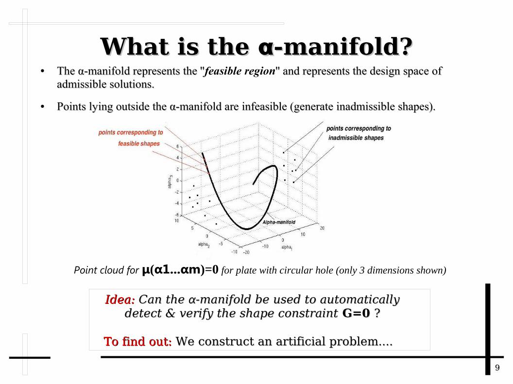
What is the What is the αα-manifold?-manifold?● The The α-manifold represents the ''α-manifold represents the ''feasible region'' and represents the design space of '' and represents the design space of

admissible solutions.admissible solutions.

● Points lying outside the α-manifold are infeasible (generate inadmissible shapes).Points lying outside the α-manifold are infeasible (generate inadmissible shapes).

Point cloud for μ(α1...αm)=0 for plate with circular hole (only 3 dimensions shown)

Idea:Idea: Can the Can the αα-manifold be used to automatically -manifold be used to automatically detect & verify the shape constraintdetect & verify the shape constraint G=0 G=0 ??

To find out:To find out: We construct an artificial problem.... We construct an artificial problem....

88

α-manifolds = feasible region! (part 1)α-manifolds = feasible region! (part 1)

Plate with elliptical hole

16 geometric parameters

OPTIMIZATION PROBLEM

Image Snapshots (elliptical holes) &

POD

99

Plate with elliptical hole (sample Plate with elliptical hole (sample snapshots)snapshots)

99

α-manifolds = feasible region! (part 2)α-manifolds = feasible region! (part 2)

1010

Basic ideaBasic idea

OUR HYPOTHESES:OUR HYPOTHESES:

● The α-manifold=feasible region in shape-space, since it The α-manifold=feasible region in shape-space, since it implicitlyimplicitly represents all represents all constraintsconstraints on the geometric variables → exclusively on the geometric variables → exclusively ''admissible'' shapes. shapes.

● Dimensionality of α-manifold (Dimensionality of α-manifold (pp) = TRUE dimensionality of the design ) = TRUE dimensionality of the design domain.domain.

THEREFORE:THEREFORE:

● FIRST detect FIRST detect pp using Fukunaga-Olsen algorithm: calculating the rank of the moment matrix for the local neighborhood of the evaluation point using a polynomial basis centered around the evaluation point.

● SECOND constrain the evaluation point to STAY on the manifold during the optimization using ''Diffuse manifold walking''.

1111

Difuse Manifold ''walking''Difuse Manifold ''walking''

Prediction:- Current evaluation point P

i

- Generate nearest neighbors for Pi

- α-space Diffuse Approximation for J- Gradient-based algorithm (e.g. Quasi-Newton) → P0

i+1

Correction:- Generate nearest neighbors for P0

i+1

- α-space Diffuse Approximation for tangent-plane- Project P0

i+1 on tangent-plane → P1

i+1

Iterate till convergence → Pf

i+1

1212

α-space optimizationα-space optimization

1313

Test case 1: Renault A/C duct

α-manifolds (p=2)

Choice of 'm'

1313 bounded geometric design variables. bounded geometric design variables.

Objective: Head loss. Objective: Head loss.

1414

Test case 2: Renault A/C duct (3D)Test case 2: Renault A/C duct (3D)88 bounded geometric design variables. bounded geometric design variables.

Objectives: Head loss (inlet → outlet)Objectives: Head loss (inlet → outlet)

α-manifolds not shown (p=4)

1515

Test-case 3:Test-case 3: Renault engine inlet duct Renault engine inlet duct

8383 bounded geometric design variables. bounded geometric design variables.

Objectives: Flow rate, TumbleObjectives: Flow rate, Tumble

α-manifolds (p=3)

(a),(b),(c) and (d)

1616

Why bother calculating the Why bother calculating the indicator functions at all ??indicator functions at all ??

1717

Conclusions.....Conclusions.....● geometric parametrization → high dimensionality, non-uniform orders of magnitude, inability to separate the geometric parametrization → high dimensionality, non-uniform orders of magnitude, inability to separate the

CAD and optimization phases, unable to guarantee admissible shapes → geometric CAD and optimization phases, unable to guarantee admissible shapes → geometric ''morphing'' ''morphing'' difficult/impractical.difficult/impractical.

(1) A (1) A ''complete''''complete'' representation of structural shape using the shape indicator function. representation of structural shape using the shape indicator function.

(2) The (2) The αα--manifold → feasible region, gives true dimensionality after all shape and technological constraints have manifold → feasible region, gives true dimensionality after all shape and technological constraints have been taken into account. been taken into account.

(3) Staying on the α-manifold guarantees admissible shapes by taking all these hidden constraints and (3) Staying on the α-manifold guarantees admissible shapes by taking all these hidden constraints and relationships between geometric parameters into account implicitly relationships between geometric parameters into account implicitly (assumption of convexity)(assumption of convexity)..

(4) We bring the problem dimensionality down from several dozen /hundred geometric parameters to a FEW local (4) We bring the problem dimensionality down from several dozen /hundred geometric parameters to a FEW local parameters (parameters (2-3 in a 86 geometric parameter 3D test case)2-3 in a 86 geometric parameter 3D test case)..

● ''diffuse walking''''diffuse walking'' forces the evaluation point to stay on the α-manifold using a local Diffuse Approximation. forces the evaluation point to stay on the α-manifold using a local Diffuse Approximation.

● Approach was successfully applied to 2 different test-cases and a third case is under investogation.

Future work: Future work:

Investigate α-manifolds in greater detail, full mathematical development, continuity?Investigate α-manifolds in greater detail, full mathematical development, continuity?

Improve indicator function → same precision with a lower resolution?Improve indicator function → same precision with a lower resolution?

Combining the approach with a POD-based ROM (POD,CPOD,etc).Combining the approach with a POD-based ROM (POD,CPOD,etc).

Extension of α-space walking to multi-objective optimization. Extension of α-space walking to multi-objective optimization.