optimality and diversi–ability of mean variance and arbitrage … · optimality and...

Optimality and Diversiability of MeanVariance and Arbitrage Pricing Portfolios

M. Hashem Pesaran Paolo Za¤aroni

University of Cambridge Imperial College LondonCIMF and USC and CIMF

August 2010

Pesaran and Za¤aroni Optimality and Diversiability

Agenda

Focus of this paper: large N characterization ofmean-variance and arbitrage-pricing portfolios.

Set-up: dynamic factor model.

Results for portfolios weights and return (Theorems),abstracts from estimation uncertainty.

Discussion of implications for:

Diversication and granularity.Role of factorsconditional distribution.Limit approximations.Short-selling.Sub-optimal trading strategies.


This papers contributions

The paper shows newresults for MV and AP tradingstrategies:

(i) It extends known results on diversication (common versusidiosyncratic risk) of MV and AP portfolios to non-exactpricing cases.

(ii) It characterizes asymptotic behaviour of portfolio weights:in non-exact pricing cases MV and AP portfolio weightsasymptotically equivalent and, moreover, functionallyindependent of factors conditional moments

(iii) (technical) provides primitive conditions on asset returnsdistribution that extends typical high-level assumptions usedin asset pricing literature.


Remark 1. Our analysis here abstracts from estimation:results are pointwise in t and we let N ! ∞ (no doubleasymptotics but cross-sectional asymptotics).

Remark 2. Generally speaking, our analysis sheds light on theissue of how to construct a market-beta neutral portfolio?One needs to identify and estimate accurately factor loadingscorresponding to strong factors! Nothing else matters.


A factor model of asset returns

Set-up: dynamic factor model: N-dimensional vector ofasset returns rt driven by a k 1 vector of common factorsand the N 1 vector of idiosyncratic components: k is xedas N ! ∞.

rt r0,t1e = µt1 + Bzt + εt

where A(N ),t [Ni=1Ai .

[[Ni=1Ait

[ At , so that

rt 2 A(N ),t for any NBoth factors and idiosyncratic shocks conditionallyheteroskedastic with zero conditional means

zt j A(N ),t1 (0,Ωt1), εt j A(N ),t1 (0,Gt1), (1)

k k matrix Ωt > 0, N N matrix Gt > 0 with Ht = G1t .It can be alternatively assumed zt j A(N ),t1 (0, Ik ) withBt = BΩ

12t .


Covariance matrix of asset returns

Gt need not be diagonal. Even bounded max eigenvaluecondition assumed by Chamberlain and Rothschild (1983) notrequired. We only need εt to be cross sectionally weaklydependent in the sense discussed in Chudik, Pesaran, andTosetti (2010). that allows ρ(Gt ) = O(Nα), for α < 1.

Asset return conditional variance-covariance matrix follows as:

Eh( rt r0,t1eµt1)( rt r0,t1e µt1)

0 j A(N ),t1i

= Σt1 = BΩt1 B0 +Gt1.

No need to specify any parametric form for H1t and Ωt .

Our set up nests various dynamic factor models withtime-varying conditional second moment: Diebold and Nerlove(1989), Harvey et al (1994), King et al (1994), Chib et al(2002), Fiorentini et al (2004), Connor et al (2006) amongothers.


Conditional means of asset returns

Conditional mean of the asset returns:

E (rt r0,t1e j A(N ),t1) µt1 = vt1 +B λt1,

Here:

vt1 pricing error,λt1 factor risk premia,

B factor loadings.

Assume vt row-wise independent from B, and Ht .Given the focus of the analysis, we take specications of µt1and vt1 as given.Dynamics can be allowed for through serial correlations inλt1.


APT Restrictions

APT starts from

µt1 = Bλt1 + vt1, (2)

whereλt1 =

B0Ht1B

1 B0Ht1µt1 (3)

is the GLS estimator and the regression residuals vt1 satisesB0Ht vt1 = 0.We make assumptions on population quantities λt1, vt1rather than on sample quantities λt1, vt1 given our aim ofestablishing limit of portfolio weights and portfolios returns.


B = ( β1, ..., βN )0 N k matrix of factor loadings such that

as N ! ∞:

N1B0e!p µβ, N1B0HtB!p Dt > 0. (4)

e = (1, 1, ..., 1)0. This result require row-wise independenceof B from Ht , εtFactors are strong in the sense that B0B = Op(N)Great deal of cross-sectional dependence is permitted.Primitive conditions are provided.

Can generalize to heterogeneous non-random B.


Three assumptions about pricing errors

Assumption on pricing consequences of di¤erent no-arbitragerestrictions (recall µt= Bλt+vt).(i) exact pricing: for any N

vt = 0.

(ii) asymptotic arbitrage pricing: as N ! ∞

e0iHtvt = Op(N 12 ), N

12 e0Htvt !p ct , v0tHtvt !p dt .

(iii) unconstrained (no arbitrage): as N ! ∞

e0iHt vt = Op(1),e0Ht vtN

!p ct ,v0tHt vtN

!p dt .

When exact pricing condition holds, our factor model isCAPM/intertemporal CAPM.


Turning to arbitrage pricing, note that under APT we shouldnot be able to nd a portfolio wt such that as N ! ∞

varhw0t1(rt r0te) j A(N ),t1

i! 0, w0t1µt1 v > 0 a.s.

otherwise there will be possibility of making unabounded riskfree returns. Under this setting we must have

v0tHt vt = v0t

Ht HtB(B0HtB)1B0Ht

vt = Op(1). (5)

Our conditions on vt ,B,Ht is slightly stronger than requiredby APT (we require the existence of limits rather than upperbounds).


Further limit conditions are required such that as N ! ∞,

e0HteN

!p at > 0, (6)

B0HtBN

!p Dt > 0, (see above) (7)

B0HtHtBN

!p Et 0, (8)

B0Htei = Op(1), e0Htei = Op(1) (9)

where ei is the i th column of the identity matrix IN .


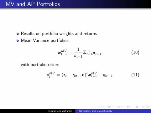
MV and AP Portfolios

Results on portfolio weights and returns

Mean-Variance portfolios:

wMVt1 =1

κt1Σ1t1µt1. (10)

with portfolio return

ρMVt = (rt r0t1e)0wMVt1 + r0t1. (11)


Arbitrage-Pricing portfolios: used to establish APT (seeIngersoll, 1984, Theorem 1)

wAPt1 =1

κt1Ht1vt1 (12)

with associated portfolio return

ρAPt = (rt r0t1e)0wAPt1 + r0t1. (13)

Recall that B0Ht vt1 = 0.


Relationships of MV and AP portfolios

To clarify analogies between MV and AP portfolios, set

Σ1t = Ht HtB(B0HtB)1B0Ht ,as compared to

Σ1t = Ht HtB(N1Ω1t +N1 B0HtB)

1N1B0Ht .

Then for any nite N > k, the AP portfolio weights satisfy

wapt1 = Σ1t1vt1 = Σ1t1vt1 = Σ1t1vt1 = Σ1t1µt1.

The AP portfolio return satises

ρapt = r0,t1 + (εt + vt1)0Σ1t1vt1,

and the di¤erence between the MV and the AP portfolio returnssatises

ρmvt ρapt = ε0tΣ1t1Bλt1 + λ

0t1B

0Σ1t1B(λt1 + zt ).


Remarks:

AP expressed as function of true pricing error vt .Estimation of APT portfolio weights does not require factorrisk premia λt .

Di¤erence between MV and AP portfolio returns involves anOp(N

12 ) term ε0tΣ

1t1Bλt1, and an Op(1) term

(z0t + λ0t1)B0Σ

1t1Bλt1, irrespective of the assumed form of

no-arbitrage.

AP portfolio return independent of the factors and their riskpremia for any N.

Under exact pricing ρAPt = r0t1.


A well diversied portfolio

We consider a slightly di¤erent denition from Chamberlain(1983) of well-diversication.

Denition 1 (well-diversication) The portfolio w is well diversiedif

kwk!p 0 as N ! ∞.

Remark (a) Since

w0Gt1w kwk ρ(Gt1) a.s.

well-diversication of w implies that idiosyncratic risk vanishes inmean square if the maximum eigenvalue of Gt1 does not growtoo quickly.


Market neutrality

Denition 2 (asymptotic market neutrality) The portfolio w is saidto be asymptotically market (or beta) neutral if

k B0wk!p 0 as N ! ∞.

Remark (a) For the AP portfolio, Denition 2 applies for all niteN > k as well, since

B0wapt = 0, for any N > k, by construction.

Remark (b) When w satises Denition 2, contribution to portfolioreturn of both the common risk, zt , and the risk premia, λt ,vanish.Remark (c) A portfolio that satises Denition 2 need not be welldiversied, as acknowledged for instance by Hubermann (1982, p.187).Remark (d) Denition 2 relevant if the portfolio weights do notdecay to zero too quickly.


Main Theorems

(exact no-arbitrage pricing) Under the exact pricing condition(i) For any i

Nwmvit e0iHtBD1t Ω1t λt !p 0 (14)

andw apit = 0.


(ii) If it is further assumed that

N1/2e0Ht1εt j At1 !d N(0, at1),

N1/2B0Ht1εt j At1 !d N(0,Dt1),

then

ρmvt r0,t1 ! p λ0t1Ω1t1(λt1 + zt ),

µmvρ,t1 r0,t1σmvρ,t1

!! p (λ0t1Ω

1t1λt1)

12 ,

andρapt = r0,t1.


To summarize, under exact no-arbitrage pricing:

wmv is well-diversied (Denition 1), but it is not marketneutral (Denition 2). wap satises Denitions 1 for anyN > k.

The limit mv portfolio excess return, and its (ex ante) Sharperatio, are only a function of the factors characteristics.

The ap portfolio excess return is identically zero.

The mv portfolio weights are Op(N1), and a function of thefactorscharacteristics.


(asymptotic no-arbitrage pricing) In this case we have(i) For any i

N12wmvit wit !p 0

andN

12w apit wit !p 0,

wherewit = N

12 e0iHtvt (ct/bt )e0iHtBA1t µβ.


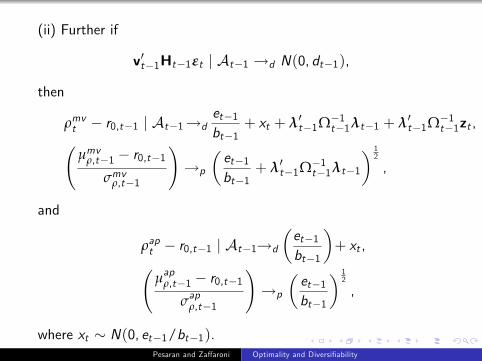
(ii) Further if

v0t1Ht1εt j At1 !d N(0, dt1),

then

ρmvt r0,t1 j At1!det1bt1

+ xt + λ0t1Ω1t1λt1 + λ0t1Ω

1t1zt ,

µmvρ,t1 r0,t1σmvρ,t1

!!p

et1bt1

+ λ0t1Ω1t1λt1

12

,

and

ρapt r0,t1 j At1!d

et1bt1

+ xt ,

µapρ,t1 r0,t1σapρ,t1

!!p

et1bt1

12

,

where xt N(0, et1/bt1).Pesaran and Za¤aroni Optimality and Diversiability

To summarize, under asymptotic no-arbitrage pricing:

wmvt is neither well-diversied nor market neutral.

The limit mv portfolio excess return, and the associated exante Sharpe ratio, are functions of both factors andasset-specic characteristics.

The ex ante Sharpe ratio is positive and bounded.

The same features apply to the limit ap portfolio excess returnwith the notable di¤erence of being functionally independentof the common factors.

In general, the limit Sharpe ratio for the ap portfolio is smallerthan that of the mv portfolio.

The mv and ap portfolio weights are both Op(N12 ). Their

limit approximation, wit , is the same and does not depend onthe distribution of the common factors, zt .


Portfolio diversication

Under the exact pricing case, the MV portfolio weights can bewritten as

wmvt = N1HtBD1t Ω1t λt +Op(N3/2),

and

wmv 0t wmvt = N1λ0tΩ1t D

1t

B0HtHtB

N

D1t Ω1

t λt +Op(N5/2)

yielding wmv 0t wmvt !p 0 as N ! ∞. Hence, in this case theMV portfolio is well-diversied in the sense of Denition 1.


The above result does not carry over to other two cases: inthe asymptotic no-arbitrage case we have

wmv 0t wmvt = v0tHtHtvt 2(ct/bt )v0tHtHtB

N

A1t µβ

+(ct/bt )2µ0βA1t

B0HtHtB

N

A1t µβ

+Op(N1/2),

which is Op(1). In this case the weights are not granular andthe possibility that one or more assets in the portfolio will begiven sizeable weights can not be ruled out even if N ! ∞.


Comparisons with some sub-optimal portfolios

We consider the global-minimum-variance (GMV) and theequal weighted (EW) portfolios.

GMV portfolio weights, wgmvt = (wgmv1t ,wgmv2t , ...,wgmvNt )0

solution to the problem:

wgmvt = argminww0Σtw

, such that w0e = 1,

yielding

wgmvt =Σ1t ee0Σ1t e

.

Well known that this portfolio does not belong to the e¢ cientfrontier, unless µi ,t1 = µt1 for all i .

This portfolio is still of interest since it does not require theestimation of expected returns. Jagannathan and Ma (2003)report comparable performance to MV portfolio.


Let

wgmvit = N1btat

e0iHte e0iHtBA1t µβ

. (15)

Then, under any of the no-arbitrage conditions listed inAssumption 5 we have:

N(wgmvit wgmvit )!p 0. (16)


For portfolio returns and the ex ante Sharpe ratio we have underexact no-arbitrage, for a random variable gt N(0, at1/bt1),

N12 (ρgmvt r0,t1) j At1 !d gt ,

N12

µgmvρ,t1 r0,t1

σgmvρ,t1

!!p

pat1µ

0βA 1

t1Ω1t1λt1.

Under asymptotic no-arbitrage

N12 (ρgmvt r0,t1) j At1 !d gt +

ct1at1

,

µgmvρ,t1 r0,t1

σgmvρ,t1

!!p

ct1pat1bt1

.


For the EW portfolio, dened by wewt = N1e, we have

ρewt r0,t1 = N1(rt r0,t1e)0e!p µv ,t1 + µ0βλt1,

where N1e0vt !p µvt , and µewρ,t1 r0,t1

σewρ,t1

!!p

µv ,t1 + µ0β λt1

µ0βΩt1µβ

.

The EW portfolio is well-diversied, but is not market neutral.Well-diversication occurs when ρ (Gt1) = op(N).ex ante Sharpe ratio of the equal weighted portfolio isbounded in N, but need not be positive.

Relatively favourable evidence provided in the empiricalliterature for the EW portfolio (see De Miguel et al (2009))most likely is due to negative impact of estimation uncertaintyon the performance of MV and AP portfolios.


Limit portfolios

Conditional distribution of factors zt can be irrelevant, as faras form of MV limiting portfolios is concerned.

Contribution of factors risk premia λt and Ωt could vanish ata fast rate.

Empirical implication: can we avoid specifying, let aloneestimating, λt and Ωt (and set them equal to zero matrices)?


Obviously, for nite N, this implies approximation error(except for AP portfolios).

But using the limit portfolio formulae permits avoiding modeland estimation risk (namely consequences of incorrectlyspecifying and poorly estimating Ωt and λt).

This suggests (radical) shrinkage-type estimator for Σ1t .(Performance will be illustrated with Monte-Carlo exercises ina follow up estimation paper)


Short-selling

When Ht diagonal

wmvit !p hii ,t

24vit µhvt

µ0βΣ1β βi

1+ µ0βΣ1β µβ

35 ,and if the factor loadings are also mutually orthogonal,

wmvit !phii ,t

1+ µ0βΣ1β µβ

24 vit +

µβ1

σβ1

2 vit v (1)it

+....+

µβk

σβk

2(vit v (k )it )

35 .where v (j)it = µhvt

βijµβj, µhvt is a weighted average of the pricing

errors, vjt .


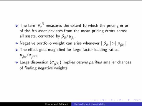
The term v (j)it measures the extent to which the pricing errorof the ith asset deviates from the mean pricing errors acrossall assets, corrected by βij/µβj .

Negative portfolio weight can arise whenever j βik j>j µβk j.The e¤ect gets magnied for large factor loading ratios,µβk/σ

β(k ).

Large dispersion (σβ(k )) implies ceteris paribus smaller chances

of nding negative weights.


Final remarks

Conclusion: new results for MV and AP trading strategies:

(i) establish well diversication and market neutrality for MV andAP portfolios under various form of no-arbitrage (understand howto build market neutral strategies).(ii) Under certain conditions, (rst-order) limit approximation ofAP and MV portfolio weights are functionally independent fromconditional distribution of factors.(iii) Primitive conditions on asset returns distribution are derived.


Implications for

Diversication.

Relevance of factors conditional distribution.

Short-selling.

Practical implementation of MV/AP portfolios (no need toestimate conditional mean and covariance of factors, althoughwe do need estimation of factors!)


Agenda of future research:

This paper presents characterization of MV/AP trading strategieswithout model and estimation risk. We are now looking at extentto which these properties are preserved when we allow for both(double asymptotics in N,T ).


optimality and diversi–ability of mean variance and arbitrage … · optimality and...

Documents