Optimal Transport and Wasserstein Distance

The Wasserstein distance — which arises from the idea of optimal transport — is being usedmore and more in Statistics and Machine Learning. In these notes we review some of thebasics about this topic. Two good references for this topic are:

Kolouri, Soheil, et al. Optimal Mass Transport: Signal processing and machine-learningapplications. IEEE Signal Processing Magazine 34.4 (2017): 43-59.

Villani, Cedric. Topics in optimal transportation. No. 58. American Mathematical Soc.,2003.

As usual, you can find a wealth of information on the web.

1 Introduction

Let X ∼ P and Y ∼ Q and let the densities be p and q. We assume that X, Y ∈ Rd. Wehave already seen that there are many ways to define a distance between P and Q such as:

Total Variation : supA|P (A)−Q(A)| = 1

2

∫|p− q|

Hellinger :

√∫(√p−√q)2

L2 :

∫(p− q)2

χ2 :

∫(p− q)2

q.

These distances are all useful, but they have some drawbacks:

1. We cannot use them to compare P and Q when one is discrete and the other is con-tinuous. For example, suppose that P is uniform on [0, 1] and that Q is uniform onthe finite set {0, 1/N, 2/N, . . . , 1}. Practically speaking, there is little difference be-tween these distributions. But the total variation distance is 1 (which is the largestthe distance can be). The Wasserstein distance is 1/N which seems quite reasonable.

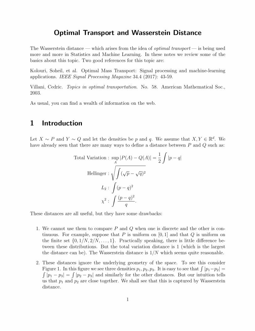
2. These distances ignore the underlying geometry of the space. To see this considerFigure 1. In this figure we see three densities p1, p2, p3. It is easy to see that

∫|p1−p2| =∫

|p1 − p3| =∫|p2 − p3| and similarly for the other distances. But our intuition tells

us that p1 and p2 are close together. We shall see that this is captured by Wassersteindistance.

1

−3 −2 −1 0 1 2 3 −3 −2 −1 0 1 2 3 −3 −2 −1 0 1 2 3

Figure 1: Three densities p1, p2, p3. Each pair has the same distance in L1, L2, Hellingeretc. But in Wasserstein distance, p1 and p2 are close.

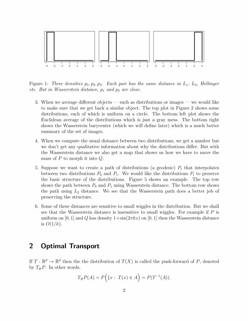
3. When we average different objects — such as distributions or images — we would liketo make sure that we get back a similar object. The top plot in Figure 2 shows somedistributions, each of which is uniform on a circle. The bottom left plot shows theEuclidean average of the distributions which is just a gray mess. The bottom rightshows the Wasserstein barycenter (which we will define later) which is a much bettersummary of the set of images.

4. When we compute the usual distance between two distributions, we get a number butwe don’t get any qualitative information about why the distributions differ. But withthe Wasserstein distance we also get a map that shows us how we have to move themass of P to morph it into Q.

5. Suppose we want to create a path of distributions (a geodesic) Pt that interpolatesbetween two distributions P0 and P1. We would like the distributions Pt to preservethe basic structure of the distributions. Figure 5 shows an example. The top rowshows the path between P0 and P1 using Wasserstein distance. The bottom row showsthe path using L2 distance. We see that the Wasserstein path does a better job ofpreserving the structure.

6. Some of these distances are sensitive to small wiggles in the distribution. But we shallsee that the Wasserstein distance is insensitive to small wiggles. For example if P isuniform on [0, 1] and Q has density 1+sin(2πkx) on [0, 1] then the Wasserstein distanceis O(1/k).

2 Optimal Transport

If T : Rd → Rd then the the distribution of T (X) is called the push-forward of P , denotedby T#P . In other words,

T#P (A) = P({x : T (x) ∈ A

)= P (T−1(A)).

2

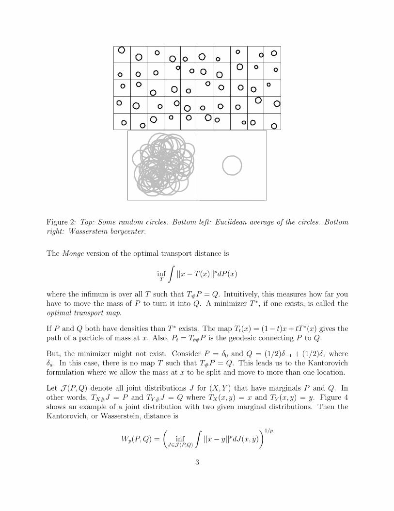
Figure 2: Top: Some random circles. Bottom left: Euclidean average of the circles. Bottomright: Wasserstein barycenter.

The Monge version of the optimal transport distance is

infT

∫||x− T (x)||pdP (x)

where the infimum is over all T such that T#P = Q. Intuitively, this measures how far youhave to move the mass of P to turn it into Q. A minimizer T ∗, if one exists, is called theoptimal transport map.

If P and Q both have densities than T ∗ exists. The map Tt(x) = (1− t)x+ tT ∗(x) gives thepath of a particle of mass at x. Also, Pt = Tt#P is the geodesic connecting P to Q.

But, the minimizer might not exist. Consider P = δ0 and Q = (1/2)δ−1 + (1/2)δ1 whereδa. In this case, there is no map T such that T#P = Q. This leads us to the Kantorovichformulation where we allow the mass at x to be split and move to more than one location.

Let J (P,Q) denote all joint distributions J for (X, Y ) that have marginals P and Q. Inother words, TX#J = P and TY#J = Q where TX(x, y) = x and TY (x, y) = y. Figure 4shows an example of a joint distribution with two given marginal distributions. Then theKantorovich, or Wasserstein, distance is

Wp(P,Q) =

(inf

J∈J (P,Q)

∫||x− y||pdJ(x, y)

)1/p

3

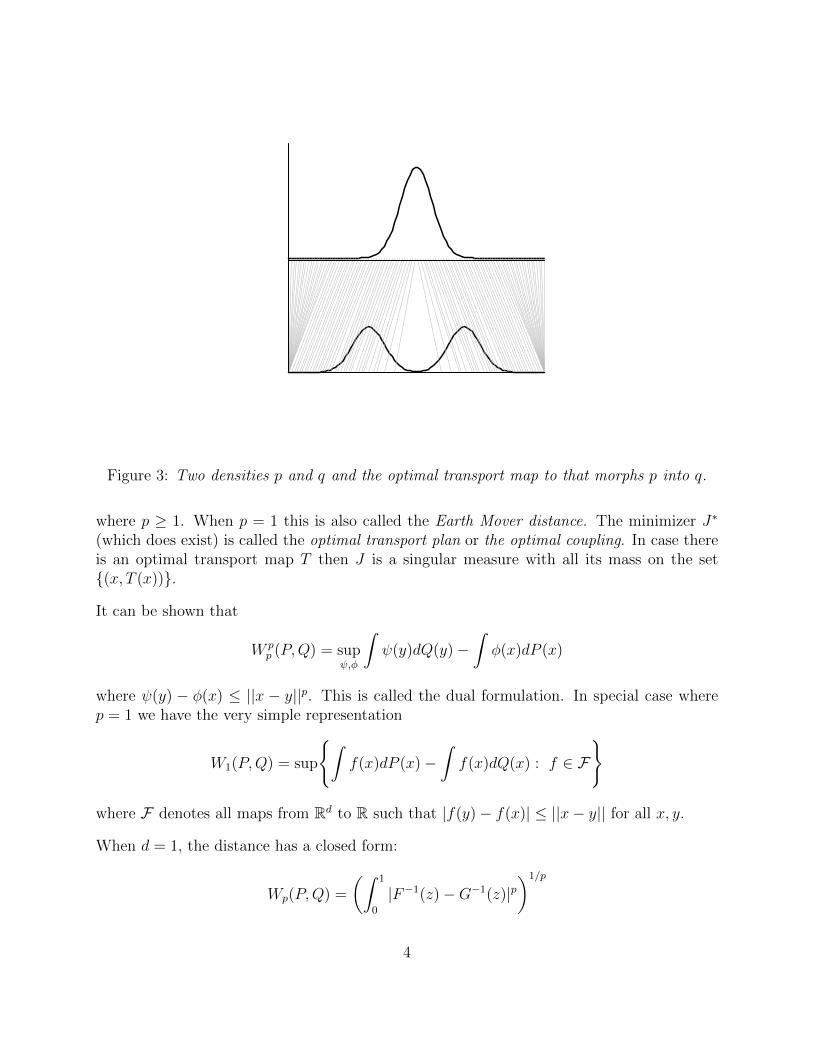
Figure 3: Two densities p and q and the optimal transport map to that morphs p into q.

where p ≥ 1. When p = 1 this is also called the Earth Mover distance. The minimizer J∗

(which does exist) is called the optimal transport plan or the optimal coupling. In case thereis an optimal transport map T then J is a singular measure with all its mass on the set{(x, T (x))}.

It can be shown that

W pp (P,Q) = sup

ψ,φ

∫ψ(y)dQ(y)−

∫φ(x)dP (x)

where ψ(y) − φ(x) ≤ ||x − y||p. This is called the dual formulation. In special case wherep = 1 we have the very simple representation

W1(P,Q) = sup

{∫f(x)dP (x)−

∫f(x)dQ(x) : f ∈ F

}

where F denotes all maps from Rd to R such that |f(y)− f(x)| ≤ ||x− y|| for all x, y.

When d = 1, the distance has a closed form:

Wp(P,Q) =

(∫ 1

0

|F−1(z)−G−1(z)|p)1/p

4

Figure 4: This plot shows one joint distribution J with a given X marginal and a given Ymarginal. Generally, there are many such joint distributions. Image credit: Wikipedia.

and F and G are the cdf’s of P and Q. If P is the empirical distribution of a datasetX1, . . . , Xn and Q is the empirical distribution of another dataset Y1, . . . , Yn of the samesize, then the distance takes a very simple function of the order statistics:

Wp(P,Q) =

(n∑i=1

||X(i) − Y(i)||p)1/p

.

An interesting special case occurs for Normal distributions. If P = N(µ1,Σ1) and Q =N(µ2,Σ2) then

W 2(P,Q) = ||µ1 − µ2||2 +B2(Σ1,Σ2)

whereB2(Σ1,Σ2) = tr(Σ1) + tr(Σ2)− 2tr

[(Σ

1/21 Σ2Σ

1/21 )1/2

].

There is a connection between Wasserstein distance and L1 distance (Indyk and Thaper2003). Suppose that P and Q are supported on [0, 1]d. Let G1, G2, . . . be a dyadic sequenceof cubic partitions where each cube in Gi has side length 1/2i. Let p(i) and q(i) be themultinomials from P and Q one grid Gi. Fix ε > 0 and let k = log(2d/ε). Then

W1(P,Q) ≤ 2dm∑i=1

1

2i||p(i) − q(i)||1 +

ε

2. (1)

5

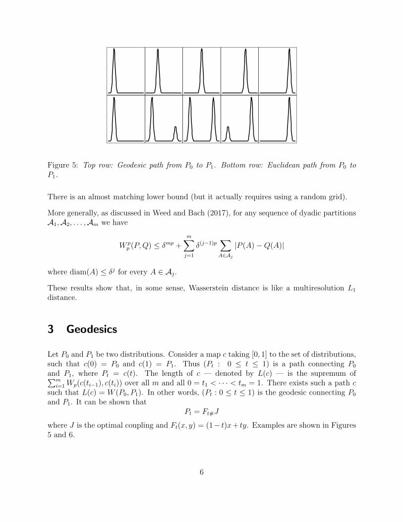
Figure 5: Top row: Geodesic path from P0 to P1. Bottom row: Euclidean path from P0 toP1.

There is an almost matching lower bound (but it actually requires using a random grid).

More generally, as discussed in Weed and Bach (2017), for any sequence of dyadic partitionsA1,A2, . . . ,Am we have

W pp (P,Q) ≤ δmp +

m∑j=1

δ(j−1)p∑A∈Aj

|P (A)−Q(A)|

where diam(A) ≤ δj for every A ∈ Aj.

These results show that, in some sense, Wasserstein distance is like a multiresolution L1

distance.

3 Geodesics

Let P0 and P1 be two distributions. Consider a map c taking [0, 1] to the set of distributions,such that c(0) = P0 and c(1) = P1. Thus (Pt : 0 ≤ t ≤ 1) is a path connecting P0

and P1, where Pt = c(t). The length of c — denoted by L(c) — is the supremum of∑mi=1Wp(c(ti−1), c(ti)) over all m and all 0 = t1 < · · · < tm = 1. There exists such a path c

such that L(c) = W (P0, P1). In other words, (Pt : 0 ≤ t ≤ 1) is the geodesic connecting P0

and P1. It can be shown thatPt = Ft#J

where J is the optimal coupling and Ft(x, y) = (1− t)x+ ty. Examples are shown in Figures5 and 6.

6

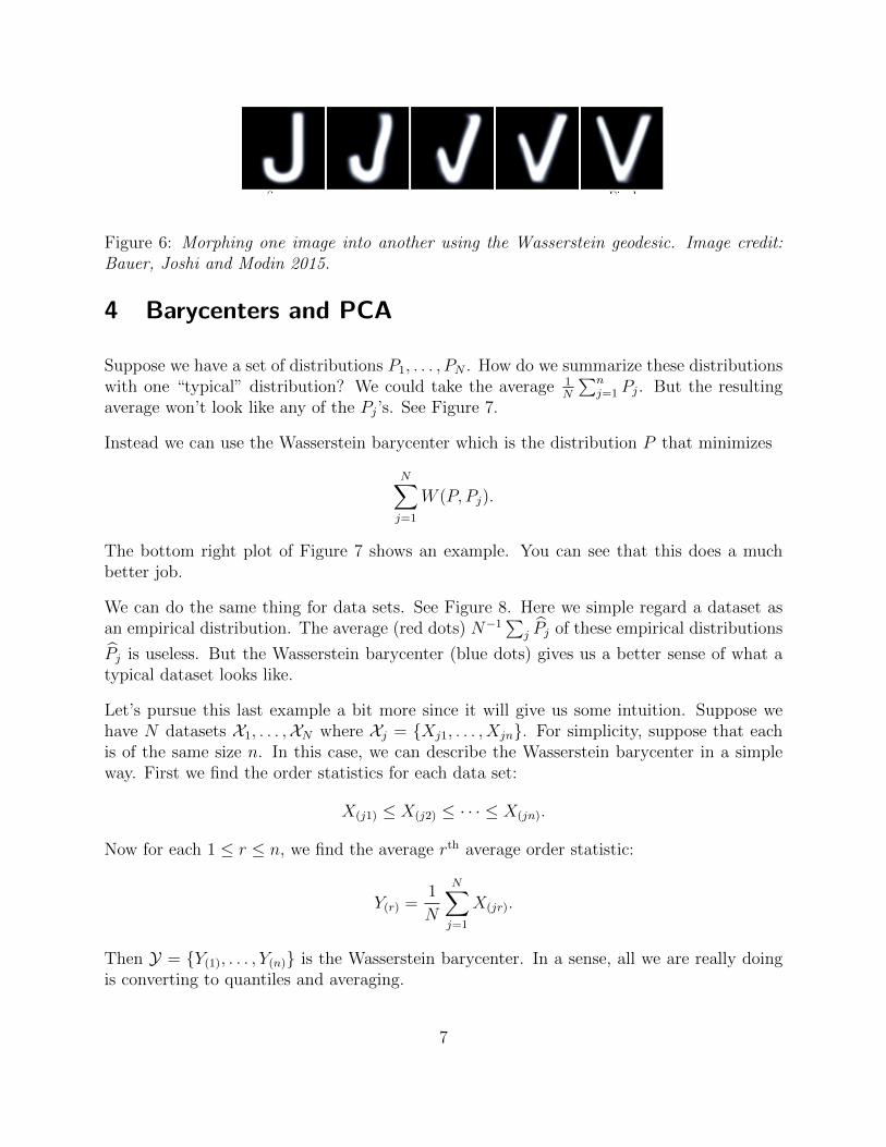
Figure 6: Morphing one image into another using the Wasserstein geodesic. Image credit:Bauer, Joshi and Modin 2015.

4 Barycenters and PCA

Suppose we have a set of distributions P1, . . . , PN . How do we summarize these distributionswith one “typical” distribution? We could take the average 1

N

∑nj=1 Pj. But the resulting

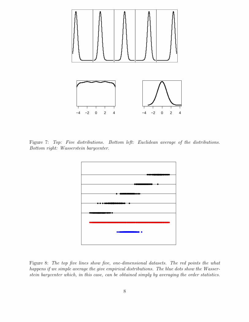
average won’t look like any of the Pj’s. See Figure 7.

Instead we can use the Wasserstein barycenter which is the distribution P that minimizes

N∑j=1

W (P, Pj).

The bottom right plot of Figure 7 shows an example. You can see that this does a muchbetter job.

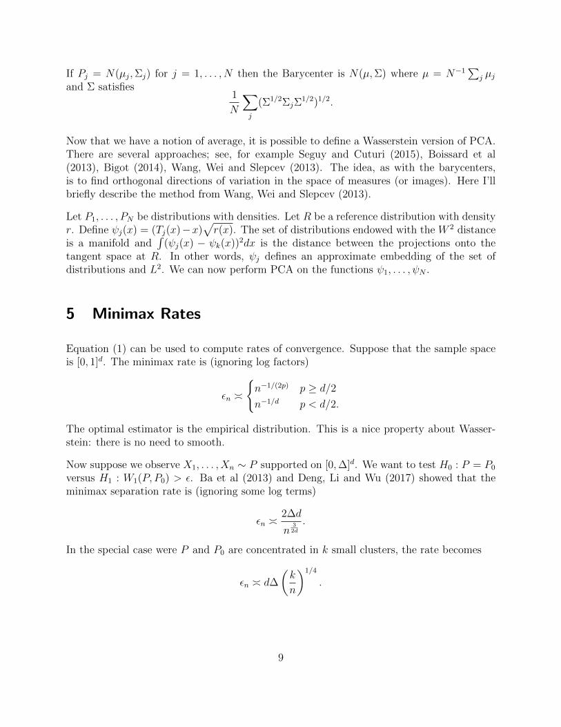
We can do the same thing for data sets. See Figure 8. Here we simple regard a dataset asan empirical distribution. The average (red dots) N−1

∑j P̂j of these empirical distributions

P̂j is useless. But the Wasserstein barycenter (blue dots) gives us a better sense of what atypical dataset looks like.

Let’s pursue this last example a bit more since it will give us some intuition. Suppose wehave N datasets X1, . . . ,XN where Xj = {Xj1, . . . , Xjn}. For simplicity, suppose that eachis of the same size n. In this case, we can describe the Wasserstein barycenter in a simpleway. First we find the order statistics for each data set:

X(j1) ≤ X(j2) ≤ · · · ≤ X(jn).

Now for each 1 ≤ r ≤ n, we find the average rth average order statistic:

Y(r) =1

N

N∑j=1

X(jr).

Then Y = {Y(1), . . . , Y(n)} is the Wasserstein barycenter. In a sense, all we are really doingis converting to quantiles and averaging.

7

−4 −2 0 2 4 −4 −2 0 2 4

Figure 7: Top: Five distributions. Bottom left: Euclidean average of the distributions.Bottom right: Wasserstein barycenter.

●● ●● ● ●●● ●● ●● ●●● ●●● ● ●● ●● ● ●●● ●● ●● ● ●●● ●● ●● ● ●● ● ● ●●●●● ● ● ●●● ●● ● ●● ● ●●● ●●● ●●●● ●●● ● ●● ●● ●●●●●● ●● ●●● ● ● ●●●●● ●●● ●

●●● ● ● ●●● ●● ● ●●● ●● ●● ● ●●● ●●● ● ●● ● ●●● ● ●● ●● ●●●● ● ●●●● ● ●●●● ●●● ●● ● ●● ● ●●●● ●● ●●● ●● ●● ●●●● ●●● ●●●● ●● ● ●● ●● ●● ●● ● ●● ● ●

●● ●●●● ●●● ●●● ●●●● ● ● ● ●●●● ●● ● ●●●● ●● ●● ● ● ●●● ●● ●●●● ●●● ●●●●●●● ●● ● ●● ●● ●●●● ●●●● ●● ●●● ● ●● ● ●● ● ●●●● ● ●● ●●● ●● ● ●● ● ●●

●●●● ●●● ●● ●●● ●●● ● ●●● ●●●● ●●● ●● ● ●●● ●● ● ●●● ●●●●● ●●●● ●●● ●●● ● ●●●● ●●● ●● ●● ● ●●●●● ●● ● ●●●● ●●●● ●●● ●● ●●● ●●● ●●●●● ●●

● ●● ●●●● ●● ●● ●● ●●● ●●● ● ●● ●●● ● ●●● ● ● ●●●●● ●● ●● ●● ●● ●●● ● ● ●● ●●● ●● ● ●●● ● ●●● ●●● ● ●●● ●● ● ●● ●● ●●●● ● ●● ● ● ●● ●● ●●● ● ●● ●●●

●● ●● ● ●●● ●● ●● ●●● ●●● ● ●● ●● ● ●●● ●● ●● ● ●●● ●● ●● ● ●● ● ● ●●●●● ● ● ●●● ●● ● ●● ● ●●● ●●● ●●●● ●●● ● ●● ●● ●●●●●● ●● ●●● ● ● ●●●●● ●●● ● ●●● ● ● ●●● ●● ● ●●● ●● ●● ● ●●● ●●● ● ●● ● ●●● ● ●● ●● ●●●● ● ●●●● ● ●●●● ●●● ●● ● ●● ● ●●●● ●● ●●● ●● ●● ●●●● ●●● ●●●● ●● ● ●● ●● ●● ●● ● ●● ● ● ●● ●●●● ●●● ●●● ●●●● ● ● ● ●●●● ●● ● ●●●● ●● ●● ● ● ●●● ●● ●●●● ●●● ●●●●●●● ●● ● ●● ●● ●●●● ●●●● ●● ●●● ● ●● ● ●● ● ●●●● ● ●● ●●● ●● ● ●● ● ●● ●●●● ●●● ●● ●●● ●●● ● ●●● ●●●● ●●● ●● ● ●●● ●● ● ●●● ●●●●● ●●●● ●●● ●●● ● ●●●● ●●● ●● ●● ● ●●●●● ●● ● ●●●● ●●●● ●●● ●● ●●● ●●● ●●●●● ●● ● ●● ●●●● ●● ●● ●● ●●● ●●● ● ●● ●●● ● ●●● ● ● ●●●●● ●● ●● ●● ●● ●●● ● ● ●● ●●● ●● ● ●●● ● ●●● ●●● ● ●●● ●● ● ●● ●● ●●●● ● ●● ● ● ●● ●● ●●● ● ●● ●●●

● ●●●●●●●●●●●●●●●●●●●●●●●●●●●●●●●●●●●●●●●●●●●●●●●●●●●●●●●●●●●●●●●●●●●●●●●●●●●●●●●●●●●●●●●●●●●●●●●●●● ●

Figure 8: The top five lines show five, one-dimensional datasets. The red points the whathappens if we simple average the give empirical distributions. The blue dots show the Wasser-stein barycenter which, in this case, can be obtained simply by averaging the order statistics.

8

If Pj = N(µj,Σj) for j = 1, . . . , N then the Barycenter is N(µ,Σ) where µ = N−1∑

j µjand Σ satisfies

1

N

∑j

(Σ1/2ΣjΣ1/2)1/2.

Now that we have a notion of average, it is possible to define a Wasserstein version of PCA.There are several approaches; see, for example Seguy and Cuturi (2015), Boissard et al(2013), Bigot (2014), Wang, Wei and Slepcev (2013). The idea, as with the barycenters,is to find orthogonal directions of variation in the space of measures (or images). Here I’llbriefly describe the method from Wang, Wei and Slepcev (2013).

Let P1, . . . , PN be distributions with densities. Let R be a reference distribution with densityr. Define ψj(x) = (Tj(x)−x)

√r(x). The set of distributions endowed with the W 2 distance

is a manifold and∫

(ψj(x) − ψk(x))2dx is the distance between the projections onto thetangent space at R. In other words, ψj defines an approximate embedding of the set ofdistributions and L2. We can now perform PCA on the functions ψ1, . . . , ψN .

5 Minimax Rates

Equation (1) can be used to compute rates of convergence. Suppose that the sample spaceis [0, 1]d. The minimax rate is (ignoring log factors)

εn �

{n−1/(2p) p ≥ d/2

n−1/d p < d/2.

The optimal estimator is the empirical distribution. This is a nice property about Wasser-stein: there is no need to smooth.

Now suppose we observe X1, . . . , Xn ∼ P supported on [0,∆]d. We want to test H0 : P = P0

versus H1 : W1(P, P0) > ε. Ba et al (2013) and Deng, Li and Wu (2017) showed that theminimax separation rate is (ignoring some log terms)

εn �2∆d

n32d

.

In the special case were P and P0 are concentrated in k small clusters, the rate becomes

εn � d∆

(k

n

)1/4

.

9

6 Confidence Intervals

How do we get hypothesis tests and confidence intervals for the Wasserstein distance? Usu-ally, we would use some sort of central limit theorem. Such results are available when d = 1but are elusive in general.

del Barrio and Loubes (2017) show that

√n(W 2

2 (P, Pn)− E[W 22 (P, Pn)]) N(0, σ2(P ))

for some σ2(P ). And, in the two sample case√nm

n+m

(W 2

2 (Pn, Qm)− E[W 22 (Pn, Qm)]

) N(0, σ2(P,Q))

for some σ2(P,Q). Unfortunately, these results do not give a confidence interval for W (P,Q)since the limit is centered around E[W 2

2 (Pn, Qm)] instead of W 22 (P,Q). However, del Barrio,

Gordaliza and Loubes (2018) show that if some smoothness assumptions holds, then thedistribution centers around W 2

2 (P,Q). More generally, Tudor, Siva and Larry have a finitesample confidence interval for W (P,Q) without any conditions.

All this is for d = 1. The case d > 1 seems to be unsolved.

Another interesting case is when the support X = {x1, . . . , xk} is a finite metric space. Inthis case, Sommerfeld and Munk (2017) obtained some precise results. First, they showedthat (

nm

n+m

) 12p

Wp(Pn, Qm) (

maxu〈G, u〉

)1/pG is a mean 0 Gaussian random vector and u varies over a convex set. By itself, this doesnot yield a confidence set. But they showed that the distribution can be approximated bysubsampling, where the subsamples of size m with m→∞ and m = o(n).

You might wonder why the usual bootstrap does not work. The reason is that the map(P,Q) 7→ W p

p (P,Q) is not Hadamard differentiable. This means that the map does nothave smooth derivatives. In general, the problem of constructing confidence intervals forWasserstein distance is unsolved.

7 Robustness

One problem with the Wasserstein distance is that it is not robust. To see this, note thatW (P, (1− ε)P + εδx)→∞ as x→∞.

10

However, a partial solution to the robustness problem is available due to Alvarez-Esteban,del Barrio, Cuesta Albertos and Matran (2008). They define the α-trimmed Wassersteindistance

τ(P,Q) = infAW2(PA, QA)

where PA(·) = P (A⋂·)/P (A), QA(·) = Q(A

⋂·)/Q(A) and A varies over all sets such that

P (A) ≥ 1− α and Q(A) ≥ 1− α. When d = 1, they show that

τ(P,Q) = infA

(1

1− α

∫A

(F−1(t)−G−1(t))2dt)1/2

where A varies over all sets with Lebesgue measure 1− α.

8 Inference From Simulations

Suppose we have a parametric model (Pθ : θ ∈ Θ). We can estimate θ using the likelihoodfunction

∏i pθ(Xi). But in some cases we cannot actually evaluate pθ. Instead, we can

simulate from Pθ. This happens quite often, for example, in astronomy and climate science.Berntom et al (2017) suggest replacing maximum likelihood with minimum Wassersteindistance. That is, given data X1, . . . , Xn we use

θ̂ = argminθ

W (Pθ, Pn)

where Pn is the ampirical measure. We estimate W (Pθ, Pn) by W (QN , Pn) where QN is theempirical measure based on a sample Z1, . . . , ZN ∼ Pθ.

9 Computing the Distance

We saw that, when d = 1,

Wp(P,Q) =

(∫ 1

0

|F−1(z)−G−1(z)|p)1/p

and F and G are the cdf’s of P and Q. If P is the empirical distribution of a datasetX1, . . . , Xn and Q is the empirical distribution of another dataset Y1, . . . , Yn of the samesize, then the distance takes a very simple function of the order statistics:

Wp(P,Q) =

(n∑i=1

||X(i) − Y(i)||p)1/p

.

11

The one dimensional case is, perhaps, the only case where computing W is easy.

For any d, if P and Q are empirical distributions — each based on n observations — then

Wp(P,Q) = infπ

(∑i

||Xi − Yπ(i)||p)1/p

where the infimum is over all permutations π. This may be solved in O(n3) time using theHungarian algorithm.

Suppose that P has density p and that Q =∑m

j=1 qjδyj is discrete. Given weights w =(w1, . . . , wm) define the power diagram V1, . . . , Vm where y ∈ Vj if y is closer to the ballB(yj, wj) and any other ball B(ys, ws). Define the map T (x) = yj when x ∈ Vj. Accordingto a result known as Bernier’s theorem, if have that P (Vj) = qj then

W2(P,Q) =

(∑j

∫Vj

||x− yj||2dP (x)

)1/2

.

The problem is: how do we choose w is that we end up with P (Vj) = qj? It was shown byAurenhammer, Hoffmann, Aronov (1998) that this corresponds to minimizing

F (w) =∑j

(qjwj −

∫Vj

[||x− yj||2 − wj]dP (x)

).

Merigot (2011) gives a multiscale method to minimize F (w).

There are a few papers (Merigot 2011 and Gerber and Maggioni 2017) use multiscale methodsfor computing the distance. These approaches make use of decompositions like those usedfor the minimax theory.

Cuturi (2013) showed that if we replace inf E||x − y||pdJ(x, y) with the regularized versioninf E||x − y||pdJ(x, y) +

∫j(x, y) log j(x, y) then a minimizer can be found using a fast,

iterative algorithm called the Sinkhorn algorithm. However, this requires discretizing thespace and it changes the metric.

Finally, recall that, if P = N(µ1,Σ1) and Q = N(µ2,Σ2) then

W 2(P,Q) = ||µ1 − µ2||2 +B2(Σ1,Σ2)

whereB2(Σ1,Σ2) = tr(Σ1) + tr(Σ2)− 2tr

[(Σ

1/21 Σ2Σ

1/21 )1/2

].

Clearly computing the distance is easy in this case.

12

10 Applications

The Wasserstein distance is now being used for many tasks in statistical machine learningincluding:

• Two-sample testing without smoothness

• goodness-of-fit

• analysis of mixture models

• image processing

• dimension reduction

• generative adversarial networks

• domain adaptation

• signal processing

The domain adaptation application is very intriguing. Suppose we have two data sets D1 ={(X1, Y1), . . . , (Xn, Yn)} and D2 = {(X ′1, Y ′1), . . . , (X ′N , Y

′N)} from two related problems. We

want to construct a predictor for the first problem. We could use just D1. But if we canfind a transport map T that makes D2 similar to D1, then we can apply the map to D2 andeffectively increase the sample size for problem 1. This kind of reasoning can be used formany statistical tasks.

11 Summary

Wasserstein distance has many nice properties and has become popular in statistics and ma-chine learning. Recently, for example, it has been used for Generative Adversarial Networks(GANs).

But the distance does have problems. First, it is hard to compute. Second, as we haveseen, we do not have a way to do inference for the distance. This reflects the fact that thedistance is not a smooth functional which is, itself not a good thing. We have also seen thatthe distance is not robust although, the trimmed version may fix this.

13