optimal detectors for transient signal … · optimal detectors for transient signal families and...
TRANSCRIPT

Uppsala UniversitySignals and Systems
OPTIMAL DETECTORS FOR
TRANSIENT SIGNAL FAMILIES
AND NONLINEAR SENSORS
Derivations and Applications
Daniel Asraf
UPPSALA UNIVERSITY 2003
Dissertation for the degree of Doctor of Philosophyin Signal Processing at Uppsala University, 2003.
ABSTRACTAsraf, D., 2003. Optimal Detectors for Transient Signal Families and NonlinearSensors: Derivations and Applications, 201 pp. Uppsala. ISBN 91-506-1664-1.
This thesis is concerned with detection of transient signal families and detectors in non-linear static sensor systems. The detection problems are treated within the framework oflikelihood ratio based binary hypothesis testing.
An analytical solution to the noncoherent detection problem is derived, which in con-trast to the classical noncoherent detector, is optimal for wideband signals. An optimal de-tector for multiple transient signals with unknown arrival times is also derived and shownto yield higher detection performance compared to the classical approach based on thegeneralized likelihood ratio test.
An application that is treated in some detail is that of ultrasonic nondestructive testing,particularly pulse-echo detection of defects in elastic solids. The defect detection problemis cast as a composite hypothesis test and a methodology, based on physical models, fordesigning statistically optimal detectors for cracks in elastic solids is presented. Detec-tors for defects with low computational complexity are also formulated based on a simplephenomenological model of the defect echoes. The performance of these detectors arecompared with the physical model-based optimal detector and is shown to yield moderateperformance degradation.
Various aspects of optimal detection in static nonlinear sensor systems are also treated,in particular the stochastic resonance (SR) phenomenon which, in this context, impliesnoise enhanced detectability. Traditionally, SR has been quantified by means of the signal-to-noise ratio (SNR) and interpreted as an increase of a system’s information processingcapability. Instead of the SNR, rigorous information theoretic distance measures, whichtruly can support the claim of noise enhanced information processing capability, are pro-posed as quantifiers for SR. Optimal detectors are formulated for two static nonlinear sen-sor systems and shown to exhibit noise enhanced detectability.
Key-words: Optimal detection, transient signals, noncoherent detection, unknown arrivaltime, ultrasonic nondestructive testing, nonlinear sensor, stochastic resonance.
Daniel Asraf, Signals and Systems, Uppsala University, P O Box 528,SE-751 20 Uppsala, Sweden. Email: [email protected].
c© Daniel Asraf 2003
ISBN 91-506-1664-1Printed in Sweden by Elanders Gotab AB, Stockholm, March 2003.Distributed by Signals and Systems, Uppsala University, Uppsala, Sweden.

To Marie my wife to beand my family
Abraham, Barbro, and Sabina

iv
AcknowledgmentsI want to express my sincere gratitude to my supervisor and dear friend, Dr. MatsGustafsson, for his valuable guidance, co-operation, encouragement and support.Mats’ broad and deep knowledge of signal processing has truly shaped me duringmy years as a Ph.D student, moreover, his enormous enthusiasm has also been agreat source of motivation. It has been a pleasure and an honor to work with Matsand I am happy that we dedicated some of our countless discussions on topics otherthan science. I sincerely hope the future will bring several more opportunities forus to work together.
I would also like to thank, Dr. John Robinson, of the Swedish Defence Re-search Agency (FOI) for helpful guidance notably during the early stages of myPh.D. studies. John’s mathematical profile brought my interest to the rigorous andpowerful tools associated with continuous-time stochastic calculus, which I hopeto further pursue, mainly for the pure interest but also so that, I too, can become“kosher”.
While working simultaneously at both FOI and the Signals and Systems grouphas proven challenging, I am deeply grateful to both institutions for allowing meto be part of their teams.
I want to thank all the people working at Signals and Systems for providing anopen and creative research environment, especially the “basement click”; FredrikLingvall, Dr. Tomas Olofsson, Dr. Ping Wu, and Professor Tadeusz Stepinski forbeing invaluable sounding-boards and enduring my constant rambling about thebiographies of various scientists. Additionally, I am very thankful to ProfessorAnders Ahlen for reading and constructively criticizing the manuscript.
I am particularly grateful to Dr. Johan Mattsson, of FOI, who provided mewith an ultrasonic scattering code and helped me to absorb rudimentary elastody-namic wave propagation and scattering theory. I would also like to acknowledgeMattias Karlsson, Dr. Peter Krylstedt, Ron Lennartsson, Ingvar Nedgard, Dr. LeifPersson, Dr. Erland Sangfeldt, and DanOberg, of FOI, for being great colleaguesand discussion partners. Due to my affiliation with FOI, I have had the opportunityto work with several international scientists, who I would like to acknowledge. Inparticular, Professor Melvin Hinich, of the University of Texas at Austin, for open-ing up my interest to other areas of signal processing and for being a dear friend.I also wish to thank Dr. Adi Bulsara, of SPAWAR Systems Center, and ProfessorLuca Gammaitoni, of the University of Perugia, for giving me a crash course onStochastic Resonance and SQUIDs but also for spicing up the atmosphere by sim-ply being themselves.

v
My reason for undertaking the “Ph.D-endeavor” begun long before I decidedto enroll as a Ph.D. student. This reason is due entirely to my parents, who broughtme up to value education, have the confidence of free thinking and appreciate theimportance of exploration and development. I am convinced that without this back-ground, my sister Sabina’s constant encouragement and support, I would have mostlikely never written this thesis.
Finally, and most importantly, I would like to express my deepest gratitude tomy fiancee, Marie, for enduring me all these years. You have been an incrediblesource of motivation with your never-ending patience and support. Thank you formaking all this worth while and for opening up my heart, my soul, and my mindto all aspects of life. Marie, words can not express enough how grateful I am andalways will be.
Daniel AsrafUppsala, February 2003.

vi

Contents
Acknowledgments iv
COMPREHENSIVE SUMMARY 1
1 Introduction 31.1 Derivations of optimal detectors . . . . .. . . . . . . . . . . . . 4
1.1.1 Detection of transient signal families in Gaussian noise . . 51.1.2 Optimal detectors in nonlinear sensor systems. . . . . . . 6
1.2 The considered application areas . .. . . . . . . . . . . . . . . . 81.2.1 Ultrasonic defect detection using piezoelectric transducers 81.2.2 Detection of a magnetic field by means of a nonlinear sensor 12
1.3 Problem formulations. . . . . . . . . . . . . . . . . . . . . . . . 171.4 Contributions . . . . . . . . . . . . . . . . . . . . . . . . . . . . 231.5 Outline of the thesis . .. . . . . . . . . . . . . . . . . . . . . . . 25
2 Signal detection 272.1 Signal detection in discrete time . .. . . . . . . . . . . . . . . . 27
2.1.1 Detection of deterministic signals in Gaussian noise . . . 292.1.2 Detection of parameterized signals in Gaussian noise . . . 322.1.3 Detection of Gaussian signals in Gaussian noise . . . . . . 36
2.2 Signal detection in continuous time .. . . . . . . . . . . . . . . . 382.2.1 Detection of deterministic signals in Gaussian noise . . . 402.2.2 Detection of parameterized signals in Gaussian noise . . . 41
2.3 Detection of non-Gaussian signals .. . . . . . . . . . . . . . . . 45
3 Defect detection in ultrasonic nondestructive testing 473.1 Elastodynamic preliminaries. . . . . . . . . . . . . . . . . . . . 47
vii

viii Contents
3.2 Modeling of the piezoelectric transducer .. . . . . . . . . . . . . 493.3 Modeling of the crack echo. . . . . . . . . . . . . . . . . . . . . 51
3.3.1 Physical model in the frequency domain . . . . . .. . . . 513.3.2 Phenomenological model in the time domain . . .. . . . 54
3.4 Modeling of clutter noise in metals. . . . . . . . . . . . . . . . . 573.5 Signal detection applied to nondestructive testing. . . . . . . . . 59
3.5.1 Physical model based crack echo detector. . . . . . . . . 603.5.2 Phenomenological model based crack echo detector. . . . 62
4 Detectors in nonlinear sensor systems 654.1 The superconducting quantum interference device .. . . . . . . . 664.2 The magneto-resistive sensor . . . . . .. . . . . . . . . . . . . . 684.3 Optimal detectors in static nonlinear sensor systems. . . . . . . . 71
4.3.1 Detectability in nonlinear sensor systems . . . . . . . . . 714.3.2 Sensor optimization for detection . .. . . . . . . . . . . 73
5 Concluding remarks and future work 75
A Background on binary hypothesis testing 77A.1 Simple and composite binary hypothesis testing . . . . . . . . . . 77A.2 Bayesian optimality. . . . . . . . . . . . . . . . . . . . . . . . . 78A.3 Neyman-Pearson optimality . . .. . . . . . . . . . . . . . . . . 80A.4 The generalized likelihood ratio strategy. . . . . . . . . . . . . . 81A.5 Detector performance evaluation . . . .. . . . . . . . . . . . . . 82
B Sufficient statistics and statistical distance measures 85B.1 Sufficient statistics . . . . . . . . . . . . . . . . . . . . . . . . . 85B.2 Statistical distance measures . . . . . .. . . . . . . . . . . . . . 88
B.2.1 Information theoretic distance measures . . . . . .. . . . 88B.2.2 The deflection ratio. . . . . . . . . . . . . . . . . . . . . 91
Bibliography 93

COMPREHENSIVE SUMMARY
1


Chapter 1Introduction
THE subjects of signal detection and information theory, in one way or an-other, deal with processing of information bearing signals in order to make
inferences concerning the information they contain. These fields trace back to theclassical work of Bayes, Gauss, Fisher [1], and Neyman and Pearson [2] but it wasnot until the 1930’s and 1940’s that Wiener [3], Shannon [4], and others, shapedthe disciplines into the form we see today.
Ever since the early dawn of signal detection and information theory, the fieldshave been actively used in a multitude of applications ranging from communica-tions and physics to economics. This progress is in many aspects due to the accessof high performing computers, which open the possibilities to process, store andcollect massive amounts of data in order to implement many of the computationallydemanding methodologies within information theory and signal detection.
Still, several applications remain that can benefit from utilizing the generalresults that have been presented within these disciplines, both when it comes topushing the envelopes of already existing methods but also in explaining and un-derstanding new phenomena.
This introductory chapter is intended to give a brief overview of the generalframework used to solve detection problems but also the different application ar-eas considered in the thesis as well as the current state-of-the-art approaches andsolutions to the problems under study. Section 1.1 outlines the generic approach tosolve detection problems based on statistical binary hypothesis testing and also howthis generic setting can be used to cast the specific problem of detecting transientsignal families and signals acquired with nonlinear sensors. Section 1.2, presentsthe two considered application areas, which are magnetic field detection and de-fect detection by means of ultrasonic nondestructive testing. The specific problems
3

4 Chapter 1: Introduction
considered in the thesis are presented in Section 1.3, followed in Section 1.4 by alist of the contributions and publications on which the thesis is based. Finally, inSection 1.5, an outline of the thesis is given.
1.1 Derivations of optimal detectors
From a purely mathematical perspective the problem of optimal signal detectionwas solved once it was connected to statistical hypothesis testing and thereby theclassical 1933 paper by Neyman and Pearson [2]. However, this insight only sig-naled the beginning of a new quest from an engineering point of view. The mainobjective of this engineering quest is to explicitly derive and apply optimal detec-tors for special, practically relevant problems.
The generic approach to solve detection problems is here briefly described byconsidering the binary hypothesis test. Binary hypothesis testing is concerned withdeciding among two possible statistical hypotheses (situations), denotedH0 andH1 respectively, by processing the outcomes,y, of a stochastic variableY . Thestochastic variableY is assumed to have two possible probability distributionsP0
andP1 underH0 andH1, respectively. This problem may be written as
H0 : Y ∼ P0
versusH1 : Y ∼ P1,
(1.1)
whereY ∼ P denotes thatY has the probability distributionP . In [2] Neymanand Pearson present a general formalism for finding a decision rule with the highestprobability of correct detection given a specified probability of false alarm. It isshown that the key quantity to compute is the likelihood ratio which is given by
L(y) =p1(y)p0(y)
, (1.2)
wherep0 andp1 are the probability density functions (pdfs) ofY under theH0 andH1 hypotheses, respectively. A comparison of the likelihood ratio to a thresholdthen yields the Neyman-Pearson optimal decision rule
δ(y) =
1 if L(y) ≥ τ
0 if L(y) < τ,(1.3)
where the thresholdτ is selected to satisfy the imposed false alarm constraint.Hence, given an observationy the decision rule in (1.3) produces eitherδ(y) = 0or δ(y) = 1 corresponding toH0 andH1, respectively. Detection strategies where

1.1. Derivations of optimal detectors 5
the likelihood ratio is compared to a threshold is also the result of a number ofother optimization criteria and is described in some more detail in Appendix A.
Thus, to derive an optimal detector oneonly has to cast the signal detectionproblem as a binary hypothesis test and then find an expression for the likelihoodratio between the considered hypotheses. Several practically relevant detectionproblems have been solved by using this methodology and proved useful in ap-plications such as radar [5, 6, 7, 8, 9, 10], sonar [5, 6, 11], and communication[12, 13].
The ambition of this thesis is to contribute to the above mentioned engineeringquest by focusing on deriving and applying optimal detectors for some problemsassociated with detecting transient signal families as well as signals acquired withnonlinear sensors.
1.1.1 Detection of transient signal families in Gaussian noise
The need to detect transient signals is apparent in applications such as radar [5, 6,7, 8, 9, 10], sonar [5, 6, 11], communication [12, 13], and ultrasonic nondestruc-tive testing (UNDT) [14], with the latter being studied in some detail in this thesis.Moreover, in many of the above mentioned applications it is common that the tran-sient signal to be detected can exhibit different waveforms from one measurementto another.
In digital communication systems this situations arises, for example, when thesymbol to be transmitted is represented by an amplitude modulated sinusoid. At thereceiver the carrier frequency and the modulation might be known but the ampli-tude and phase may not. This yields that the transient signal to be detected can berepresented by an explicit mathematical expression with the amplitude and phaseas unknown parameters.
In the radar, sonar, and UNDT applications the transient signal to be detected is,for example, generated by the back-scattered echo from a potential object impingedby a transmitted pulse. The waveform of the received target echo is dependent onthe the physical attributes involved in the scattering process such as the objectsshape, location, orientation, material, etc.
Regardless of the signal generating mechanism, the transient signal family canbe described by
S = s(θ)|θ ∈ Λ, (1.4)
wheres(θ) = [s1(θ), . . . , sN (θ)]T is a vector1 of samples from a transient signal,θrepresents explicit mathematical or underlying physical parameters andΛ is some
1In the discrete time problems treated in this thesis vectors are taken to be columnar and thesuperscriptT denotes transposition.

6 Chapter 1: Introduction
space whereθ takes its values.The problem of detecting a transient signal, randomly drawn from the family in
(1.4), and corrupted by an additive noise can be formulated as a binary hypothesistest (1.1). A discrete time formulation of (1.1) may be expressed as
H0 : Y = Vversus
H1 : Y = s(θ) + V ,(1.5)
whereY ∈ RN is a stochastic vector representing a sampled version of the ob-
served signal andV is a vector of noise samples. In statistical hypothesis testingthe problem in (1.5) is commonly referred to as a composite hypothesis test sincetheH1-hypothesis is dependent on the unknown parameterθ.
Thus, to find an optimal detector for (1.5) on the form (1.3) the likelihood rationeeds to be computed. This involves not only knowledge of the statistical prop-erties of the noiseV , and the waveforms of the signalss(θ) but also the randomlaw describing how the signalss(θ) are drawn from (1.4), i.e. the distribution ofθ on Λ. Even if all this knowledge is available and expressed by explicit mathe-matical expressions the derivation of the likelihood ratio is often a formidable taskto perform analytically. Historically, the analytical approach was the main routeto consider in order to achieve a practically useful detector, but due to the currentaccess of high performing computers alternative approaches, based on numericalsolutions, are opened up.
1.1.2 Optimal detectors in nonlinear sensor systems
Sensors are generally based on mechanisms where one physical quantity can becoupled to another, e.g. a magnetic field at the input to the sensor yields an elec-trical voltage at its output. Several of these physical mechanisms are nonlinear bynature and when designing sensors great effort and ingenuity are used to obtain alinearized regime within which the sensor is to be operated. However, in situationswhen a sensor is operated outside its linear regime, e.g. in very noisy environ-ments, the interpretation of the sensor outputs becomes more complicated. Thislimits the original usability of the sensor to reach end objectives such as detection,estimation, prediction etc.
Recently a new approach for detecting a weak harmonic signal in additiveGaussian noise, measured by a nonlinear sensor, was proposed independently byHibbset al. [15] and Rouseet al. [16]. Their method utilizes the nonlinear char-acteristics of the super conductive quantum interference device (SQUID) to detecta weak magnetic field corrupted by an additive Gaussian noise. The key step in

1.1. Derivations of optimal detectors 7
their proposed detection strategy is to “tune” the SQUID to operate in the so-calledstochastic resonance (SR) regime [17, 18].
In this context the SR effect yields the somewhat unintuitive phenomenon ofincreased detectability with increased noise strength. A generally accepted descrip-tion of the SR phenomenon is that of a noise induced performance enhancement interms of the system’s information processing capability [17, 18, 19, 20, 21]. Al-though SR has been observed in several different application areas and contexts,one of the most studied and exemplified is that of signal detection, mainly due tothe unintuitive effect of noise enhanced detection performance. Recently a similarstudy has been presented in the signal processing community where Kay poses thequestion: “Can detectability be improved by adding noise?” in a paper with thesame title [22].
As pointed out above, the approach taken by Hibbset al. [15] and Rouseetal. [16] was based on the SR phenomenon and focused less on the signal process-ing methodologies associated with optimal detection. Therefore, it is of interestto explore the potential of deriving and applying statistically optimal detectors fornonlinear sensors. The fundamental problem considered is to detect if a weak sig-nal is present in an additive Gaussian noise environment based on measurementsacquired with a nonlinear sensor. This problem is naturally cast within the frame-work of binary hypothesis testing by modeling the hypotheses in (1.1) as
H0 : Yt = gβ(Vt), 0 ≤ t ≤ Tversus
H1 : Yt = gβ(st + Vt), 0 ≤ t ≤ T.(1.6)
Herest is the signal to be detected,Vt is the additive Gaussian noise,Yt is thesensor output signal andgβ represents the nonlinear sensor, which can be “tuned”by means of the parameterβ. Obviously, even if the noiseVt is Gaussian andthe signal to be detected,st, is deterministic and known, the sensor outputYt
will be non-Gaussian under bothH0 andH1 due to the nonlinear characteristicof gβ . Generally, non-Gaussian detection problems are analytically intractable andthereby usually attracts alternative types of signal processing, e.g. wavelet decom-positions, neural networks, and higher order statistics. A comprehensive tutorialon non-Gaussian detection problems can be found in [23]. The preferred approachfor a particular problem depends on the level of knowledge that can be used indescribing the stochastic processes. In situations when little knowledge is at handone has to retreat to suboptimal techniques which are tailor made for the particularproblem. The approach taken by Hibbset al. [15] and Rouseet al. [16] can beconsidered to belong to these suboptimal techniques since their method is based onqualitative reasoning concerning the spectral characteristics of the signal and noton the likelihood ratio.

8 Chapter 1: Introduction
When the sensor transfer characteristicsgβ , the statistical properties of thenoiseVt as well as the signal to be detectedst, are all considered to be knownthere is no need to retreat to suboptimal procedures to solve (1.6). Instead theclassical statistical hypothesis testing approach can be used to construct an opti-mal likelihood ratio detector. The statistical hypothesis testing formulation of thesensor-detector problem does not only have the benefit of ensuring optimality, italso provides a framework for an information theoretic (IT) view on the sensor“tuning” problem. Moreover, as is shown in this thesis, the IT formulation yields,as a “Bonus”, a generalization of the SR phenomenon.
Due to the development of digital signal processors (DSP) ubiquitous algo-rithms can be implemented in sensor systems to tackle problems such as “tuning”and detection. The signal processing approach can in this way enhance perfor-mance of nonlinear sensor systems by expanding the sensors operating regime andhas the benefit of alleviating the constraints imposed by linearizion and therebyreducing, for example, energy consumption, complicated and costly design proce-dures, the use of expensive materials etc.
1.2 The considered application areas
In this thesis the two considered application areas are defect detection by meansof ultrasonic nondestructive testing (UNDT) and detection of magnetic fields mea-sured by means of a nonlinear magnetic sensor. Although many of the utilizedmethodologies and results presented here are of general applicability this section isintended to give an overview of the two application areas as well as a brief descrip-tion of some of the state-of-the art methods of particular interest for the problemstreated in this thesis. The considered application areas are briefly presented next.
1.2.1 Ultrasonic defect detection using piezoelectric transducers
Most transducers used for ultrasonic nondestructive testing (UNDT) are based onpiezoelectric materials due to their ability to convert electric energy to mechanicalenergy and vice versa. In this type of testing procedure, acoustic waves or pulsesin the frequency range of1 − 10 MHz, are transmitted into a test specimen andthe reflected echoes are analyzed to make inferences about the condition of thespecimen. Many materials, such as stainless steel and copper, consist of randomlyconfigured and densely packed crystals or grains. These grains, as well as othermicro-structural inhomogeneities, affect the acoustical impedance of the material.Therefore, when an acoustic pulse is emitted into a material the pulse will be scat-tered, not only by the defects, but also by a myriad of micro-structures that will

1.2. The considered application areas 9
cause the received signal to exhibit a random behavior. This signal, which is in-duced by the backscattering from the material micro-structure is commonly calledclutter.
Common UNDT objectives are to detect defects or to characterize the shape,location, and orientation of material inhomogeneities. Furthermore, material prop-erties such as density and stiffness can also be estimated by means of an UNDTsystem. These objectives are of significant importance in many industrial branchessuch as nuclear power plants, aircrafts, and construction sites, where componentsof metal, composites, and concrete are tested for flaws. Yet another vast area whereultrasonics has been found very useful is medical diagnosis. Detection of tumorsand monitoring of pregnancies (fetus) are two examples.
The main components of a typical UNDT measurement system are depictedin Figure 1.1. An electric pulser is used to excite one transducer (or an array oftransducers), which converts the electric energy into a displacement field. Thedisplacement field propagates into the test specimen where the wave is scatteredby inhomogeneities in the solid. Parts of these scattered waves are received by asingle transducer (or an array of transducers), which converts the scattered fieldinto an electric signal. The signal is amplified in a receiver and can be viewed onan oscilloscope for instantaneous visual examination or discretized and stored in acomputer.
Oscilloscope
Pulser
Receiver
Digitizer Computer
Transmitter/ReceiverTransducer
TestSpecimen
Figure 1.1: Schematic of an UNDT system.
There are three main transducer configurations used in ultrasonic contact test-ing scenarios. The applicability of the configurations depend on the end objectiveof the examination and the geometrical shape of the specimen being tested. Thesedifferent configurations are depicted in Figure 1.2 and referred to aspulse-echo,pitch-catch, and through-transmission. A common test scenario is the so-called

10 Chapter 1: Introduction
(b) (c)(a)
Figure 1.2: Different contact testing configurations: (a) pulse-echo setup, (b)pitch-catch set up, (c) through-transmission setup.
immersion testing whereby the object is immersed in water in order to achieve a“good” acoustic coupling between the object and the transducer. The UNDT con-tributions in this thesis exclusively considers the contact testing pulse-echo config-uration, which also is the most common setup in industrial applications.
The physical mechanisms from pulser to receiver can in most cases be con-sidered as linear and time invariant [14]. Thus, the whole measurement processfrom the electrical excitation pulse to the received electrical signal can be mod-eled as a series of linear time-invariant (LTI) systems. Due to the LTI properties,the systems can, mathematically, be treated individually and reconfigured whenmodeling/computing overall signal responses.
Often the operator of an UNDT system visually examines the raw signal to de-termine if a test specimen contains defects. This is a very time consuming processsince the defect echoes can be severely obscured by the clutter noise and requiresextensive experience in order to be successful in finding small defects. Moreover,this kind of screening process is colored by the operators subjectivity and ability tomaintain attention through out the inspection of large amounts of data.
In order to alleviate the burden on the operator, to increase detection perfor-mance, and to reduce subjectivity and time consumption, appropriate signal pro-cessing algorithms can be utilized to aid the operator. Such signal processing al-gorithms have mainly been designed for reducing the clutter noise in the measuredsignals. Since the grains in a material specimen being tested have fixed locations,the clutter noise signal will not vary in time, thus simple averaging of multiple mea-surements will not reduce the clutter. However, the clutter noise signal is highlydependent on the position and the frequency characteristic of the transducer. Theseeffects are employed in the two main approaches currently used for clutter suppres-sion. In the first, the spatial diversity of the material grains is utilized by performingmultiple measurements, each at a slightly different position. The resulting signals

1.2. The considered application areas 11
are then averaged yielding a reduction of the clutter. This approach relies on thefact that the echo from a large defect will not change dramatically when movingthe transducer slightly. The other approach utilizes the frequency diversity by us-ing transducers with different center frequencies, whereby the clutter componentin the signal will vary for different frequency bands while the echo from a largedefect should remain relatively constant. Thus, both these approaches rely on thequalitative insights that the echo from a large defect is relatively unchanged oversome specific frequency range as well as small shifts of the transducer position.However, these techniques are both costly and time consuming due to the need ofmultiple measurements and/or the use of several transducers.
One approach, known as split spectrum processing (SSP) [24, 25, 26, 27] uti-lizes the underlying idea in the frequency diversity approach by using one wide-band transducer and then synthetically segmenting the measured signal,y, intoseparate sub-bands using a filter bank, see Figure 1.3. These sub-band signals arethen combined, usually by some nonlinear operation, into a filtered signal, denotedz in Figure 1.3. The SSP approach is qualitative since it is not based on any explicitassumptions of the physical properties of the defects other than that the echo signalfrom a large potential defect will contain spectral energies over a wide frequencyband.
y
. .
. z
fN
f2
f1
OperationNonlinear
IFFT
IFFT
IFFT
FFT
Figure 1.3: Schematic of an SSP system. The sampled signal received from the ul-trasonic transduceryn is filtered through a digitally implemented filter bank usingthe fast Fourier transform and the filter bank outputs are then processed by somememoryless nonlinear operation.
The SSP technique is dependent on several parameters, for example, the centerfrequencies of the bandpass filters, their bandwidth, and overlap in the frequencydomain. Extensive research [24, 28, 29, 30] has been devoted to developing strate-gies for finding parameters yielding an output signal,z, which clearly shows if adefect is present. The parameter optimization is mainly complicated by the non-linear operation used to combine the output from the filter bank. One optimization

12 Chapter 1: Introduction
technique proposed in [28, 29, 30] is based on the so-called signal-to-noise ratioenhancement (SNRE), which is the ratio between the input- and the output SNR.The SNRE is defined by
SNRE=SNRIn
SNROut=
E1yn0√E0(yn0)2
/E1zn0√E0(zn0)2
(1.7)
whereyn0 andzn0 are the input and output signals, respectively,n0 is the samplenumber corresponding to the specific time instant of interest, andE0· andE1·denote the expectation underH0 andH1, respectively. The basic idea in this op-timization strategy is then simply to find the SSP parameters which maximize theSNRE in (1.7) when presented training data containing clutter contaminated defectechoes as well as only clutter.
1.2.2 Detection of a magnetic field by means of a nonlinear sensor
Magnetic sensors are useful in a wide area of application and for a variety of finalobjectives. There exist a multitude of magnetic sensor types, which are based ondifferent physical mechanisms and which are applicable in situations dependingon sensitivity requirements and environment of operation. The two types of mag-netic sensors studied in this thesis are the magneto-resistive (MR) and the superconductive quantum interference device (SQUID), which both are inherently non-linear. Common application areas for both these sensors are nondestructive testingand geomagnetism. For both these applications the main objectives are detection,localization, and classification of either objects buried in the ground or defects re-siding in components. The MR sensor, in particular, is also often used for readingthe magnetic stripe on, for example, credit cards and the SQUID sensor has beenfound very useful in naval warfare where again detection, classification and local-ization are the primary goals.
In this thesis the problem in focus is that of detecting a magnetic fieldst, con-taminated by a strong additive ambient noisevt, based on measurements,yt, fromthe MR or the SQUID sensor, see Figure 1.4.
0, st
vt
yt 0, 1+ gθ(·) δθ(yt)
Sensor Detector
Figure 1.4: Schematic block structure of a sensor-detector system.

1.2. The considered application areas 13
A complication encountered when applying these sensors in very noisy envi-ronments is their nonlinear transfer characteristics which makes it difficult to inter-pret the output signalyt. This complication is often overcome by some means ofsensor tuning where the transfer characteristic is altered so that the sensor producesvaluable output signals. In Figure 1.4 the sensor transfer characteristic is denotedgβ whereβ denotes the tuning parameter.
There are several techniques of varying degree of sophistication for tuningmagnetic sensors [31]. One simple, but efficient, way to tune a magnetic sensoris to inject a carefully chosen external magnetic field, thereby altering the work-ing point of the sensor. In this case the tuning parameterβ could, for example,correspond to the amplitude of the injected field.
A central problem is to find an appropriate value for the tuning parameterβ.This should naturally be solved with the final objective in mind in order to reachthe highest possible performance. As mentioned previously, a recently proposedmethod, presented in [15, 16], for improving the detectability of a weak harmonicsignal in additive Gaussian noise, is based on tuning a nonlinear sensor to operatein the SR regime. This approach is briefly discussed in the proceeding section.
Operating a sensor in the SR regime
The term stochastic resonance (SR) has been given to a phenomenon that mayoccur in nonlinear systems whereby some particular features of a weak input ex-citation is amplified by the assistance of a random signal, e.g. noise. This hasrendered a multitude of publications where systems have been operated in theSR regime in order to exhibit noise induced enhancement of detection perfor-mance [19, 20, 21], channel capacity [32, 33], neuronal responses [34], imageand signal processing [35, 36], etc. Due to the occurrence of SR in such a vari-ety of contexts, different characterizations (definitions) of the SR effect have beenproposed [18]. In many of these studies the quantifier for SR is tailor made for thespecific application under study to exhibit and use the desired effect.
The role of SR in sensor-detector applications is one of the main topics of thisthesis, which is further explained by an example given below. In this example thesensor is represented by a nonlinear dynamical system and the detector is intendedto operate on the output from the sensor. The particular nonlinear dynamics used inthe example is that of a double-well potential2. This particular dynamics is chosensince it is a classical example of the SR effect.
2Double-well potential means that the dynamical system has two local minima in the state space,see Figure 1.5

14 Chapter 1: Introduction
EXAMPLE 1.1: SRIN A DOUBLE-WELL SENSOR
Consider a sensor with a transfer function that can be described by the stochasticnonlinear differential equation (SNDE)
Yt = Y0 +∫ t
0
d
dyf(Yτ )dτ + st + σVt. (1.8)
Here,Yt is a stochastic process representing the sensor’s output signal,f is anonlinear function representing the double-well potential of the system,st is aperiodic excitation signal, andVt is a zero mean unit variance white Gaussiannoise scaled by the noise strength parameterσ. The input signal,st, is taken tobe harmonic and described by
s(t) = A0 cos(2πf0t), (1.9)
whereA0 determines the strength andf0 the frequency. Moreover, let the double-well potential,f , be represented by
f(x) =b
4x4 − a
2x2. (1.10)
The dynamics in (1.10) has two potential minima located at±xm = ±√
a/b.In the absence of noise, and when the system is unperturbed the minima areseparated by a potential barrier with the hight given by∆V = a2/(4b).
If the system in (1.8) is perturbed only by the harmonic signal in (1.9), thenthe potential minima are tilted up and down periodically, thereby lowering thepotential barrier separating them. If the periodic forcing is strong, i.e. largeamplitudesA0, then the system’s state will transit between the potential minimawith a rate corresponding to half the forcing frequencyf0. This type of excitationis called supra-threshold forcing and is visualized in Figure 1.5. A periodicforcing with small amplitudes,A0, will cause the system’s state to rock back andforth in one of the potential wells. This is commonly calledsub-threshold.
The output signal from the system in (1.10), when excited by a sub-thresholdperiodic forcingst, exhibits interesting behavior when altering the inherent noisestrengthσ. First consider the noise strengthσ to be small, then only few transi-tions between the potential minima will occur, generating an output signal withthe typical behavior presented in the lower left plot in Figure 1.6. On the otherhand, if the noise strength is very high, several random transitions between thepotential minima will occur, producing an output signal as in the upper left plot in

1.2. The considered application areas 15
f(x)
x
f(x)
x
f(x)
x
-x m xm
V∆
f(x)
x
Figure 1.5: The double well potential in (1.10) excited by a periodic forcing.
Figure 1.6. For a moderate noise strength the system operates in an intermediateregime where the systems state transits between the wells with a rate synchro-nized with half of the periodic forcing. This is depicted in the middle left plotin Figure 1.6. Also presented in the right column of Figure 1.6 are the powerspectra averaged over 500 realizations of the corresponding time domain signals.
Curiously, when the noise strength is increased and reaches some intermedi-ate level the sensor output signal starts to oscillate betweenxm and−xm with aperiod equivalent to half the forcing frequency. This is the SR effect, which isalso clearly visible in the frequency domain plots in Figure 1.6. Thus, if a fre-quency based detector, with a detection statistic represented by the amplitude ofthe power spectral component at half the forcing frequency, was to operate on thesensors output signal, then the detectability would be improved by adding noise.
In the light of the behavior of the signals presented in Figure 1.6 it is temptingto quantify the SR effect, and thereby the information processing capabilities ofthe system, in terms of spectrum based measures, since the barrier-crossing rate

16 Chapter 1: Introduction
0 0.5 1−20
−10
0
10
20
t [s]
xm
xm
1 3 9 300.1
1
10
f [Hz]
0 0.5 1−20
−10
0
10
20
t [s]
xm
xm
1 3 9 300.1
1
10
f [Hz]
0 0.5 1−20
−10
0
10
20
t [s]
xm
xm
1 3 9 300.1
1
10
f [Hz]
Figure 1.6: On the left the nonlinear sensor output signal is displayed for differentnoise strength parameter valuesσ (increasing values from the bottom row to thetop row). Also depicted by the dashed line is the harmonic input signal, with anormalized amplitude. On the right the corresponding power spectra based on500 realizations of the output signal is displayed.
depends critically on the noise strengthσ. Indeed, the most common way to char-acterize SR is by means of a signal-to-noise ratio (SNR) of the system’s outputsignal. This SNR is expressed in the spectral domain by exclusively consideringthe spectral component at the fundamental frequency given by the input excitation,which corresponds tof0 in Example 1.1. By assuming that the system has a sta-
1.3. Problem formulations 17
tionary solution when the excitation signalst = 0 and a cyclostationary solutionwhenst is harmonic as in (1.9), this spectral based SNR measure may be expressedas [18]
dSR =a
S0V (f0)
. (1.11)
HereS0V (f0) is the power spectral component atf0 of Yt without any periodic
excitation of the system anda = |c1|2/2π, wherec1 is the first coefficient inthe Fourier expansion
∑n∈Z
cnei2πf0nt of the ensemble averaged system responsewith a harmonic excitation of frequencyf0. Obviously, this approach makes mostsense if the system under study can be described by a SNDS as in (1.8) and theexcitation signal is harmonic. However, similar spectral based SNR measures hasalso been utilized for other types of systems and excitation signals [18].
The motivation for having a quantifier for the SR phenomenon and thereby theinformation processing capability of a nonlinear system lies not only in describingthe phenomenon but also, and more importantly, in that such a measure can serveas a cost function when optimizing system performance. In many practical appli-cations, altering of the noise strength is not an option to be considered. Instead,from a technical perspective, a similar effect can occur by “tuning” the system tooperate in the intermediate regime where the SR effect becomes pronounced. Forthe double well potential this could, for example, be made by altering the barrierhight ∆V . As mentioned, Hibbset al. [15] and Rouseet al. [16] managed tooperate a SQUID in its SR regime. At the sensor output they utilized a frequencybased detector, set to the fundamental frequency of the input signal, to detect har-monic magnetic fields. This system clearly showed better detectability with in-creased noise strength. Also, the spectral based SNR measure of the sensor outputin [15, 16] indicated a similar performance enhancement. Based on the resultsfrom these studies general conclusions of noise enhanced detection performancewere drawn. In this thesis, these types of general conclusions are reconsidered us-ing optimal detectors instead of detectors based on suboptimal detection statistics.
1.3 Problem formulations
In several applications such as digital communications, radar and sonar, the signalfamily to be detected can be modeled by an amplitude modulated sinusoid. Thus,the signal family may be expressed as
st = Aat sin(2πfct + φ) (1.12)
whereA is the amplitude,at is the envelope,fc is the carrier frequency andφ isthe phase angle. For this case the unknown parametersθ in (1.4), which spans the

18 Chapter 1: Introduction
signal family, can be various combinations ofA, fc, andφ.Due to the wide applicability of the signal family in (1.12) significant research
has been devoted to developing detectors for these types of signals, in particularwhen corrupted by an additive Gaussian noise. The resulting detection strategiesfocus on providing high performing and practical solutions to problems whereθincludes close to all permutations of the unknown parametersA, fc and φ. Acomprehensive display of several of these detectors and strategies can be foundin [5, 7, 8, 12]. Some special cases, which have received extra attention, are listedbelow:
1. A, at, fc, andφ are completely known3
2. A, at, andfc are known and deterministic andφ ∼ U [0, 2π], whereU [·, ·]denotes the uniform distribution.
3. at andfc are known and deterministic,φ ∼ U [0, 2π] andA ∼ R(σA), whereR(σ) denotes the Rayleigh distribution.
One well-known detector is thenoncoherent detector, which is applicable forthe case listed in item 2 above. However, in the derivations of the likelihood ratiofor the noncoherent detection problem it is assumed that the envelopeat satisfiesthe so-callednarrowband approximation, which can be expressed as
∫ T
0a2
t cos(4πfct + 2φ) dt = 0, ∀φ ∈ [−π, π]. (1.13)
This entails that the bandwidth of the envelope is narrow in comparison with the(carrier) frequency,f0, of the sinusoid. In the case of wideband transient signalsthe envelope can not be considered to satisfy the narrowband approximation (1.13)and thereby the classical noncoherent detector will be suboptimal. This is the topicfor the first problem statement described below.
Problem 1: Wideband noncoherent detector
The objective is to derive an expression of the likelihood ratio for the non-coherent detection problem without imposing the narrowband approximationin (1.13). The objective is also to evaluate the performance of this detectorcompared to the classical noncoherent detector to find out the performancedegradation caused by imposing the narrowband approximation.
3This case simply yields the matched filter detector which is optimal regardless of the wave formof the signal [8].

1.3. Problem formulations 19
An often encountered problem when detecting transient signals is that of un-known arrival time. This situation arises, for example, in the radar, sonar, andUNDT applications where the measured signal is generated by backscattered echo-es due to a transmitted pulse. For this scenario, the arrival time of the receivedtarget echo is mainly dependent on the location of the object to be detected.
The objective is to find a detector which can determine if there is a transientsignal, e.g. target echo, present anywhere within a measurementyT
0 = yt; t ∈[0, T ], taken over some specific time intervalt ∈ [0, T ]. As always, the keyissue in formulating such a detector is to find a detection statistic, preferably thelikelihood ratio. A common approach to obtain a detection statistic for this problemis by means of a maximum likelihood formulation [12]
maxτ∈[0,T ]
L(yT0 |τ), (1.14)
whereL(yT0 |τ) is the likelihood ratio for the case of a single pulse with known
arrival time. For the case of detecting a single pulse with ana priori known arrivaltime pdfpΥ the optimal detection statistic is given by [7, 37]
∫ T
0L(yT
0 |τ)pΥ(τ) dτ. (1.15)
An extension of the unknown arrival time problem discussed above is consid-ered in the problem statement below and treats the case when the measured signalmay consist of multiple pulses all with unknown arrival times. This scenario could,for example, also occur in the radar, sonar, and UNDT applications when there aremultiple targets generating reflected echoes or a single target located in an environ-ment with multi-path propagation. Yet another example is targets of extended spa-tial dimension with several reflecting surfaces generating multiple reflected pulseseven if only one pulse was transmitted.
Problem 2: Multiple pulses with unknown arrival timesThe objective is to first derive an expression for the likelihood ratio whenthe signal to be detected can consist of multiple transient signals with un-known arrival times. Then compare the performance of a detector based onthis likelihood ratio to one with the maximum likelihood ratio detection statis-tic in (1.14).
Generally, formulating an optimal detector for a hypothesis problem such as(1.5) requires that an accurate representation of the signal familyS in (1.4) is ac-cessible. In all practical detection problems the signals to be detected are, in one

20 Chapter 1: Introduction
way or another, generated by some underlying physical mechanisms. In some ofthese situations it is difficult to derive/obtain an explicit parameterized mathemat-ical model of the signal family. A scenario where this difficulty may emerge isthat of defect detection by means of UNDT which is the focus of the third problemstatement below. As mentioned, common approaches to test for defects by meansof a piezoelectric UNDT system are aimed at reducing the clutter noise in the mea-sured signal and does not explicitly utilize the framework of binary hypothesistesting to solve the problem. Thus, a signal detection treatment of the ultrasonicdefect detection problem seems appropriate and has the potential to contribute tothe UNDT application area. The ambition is to add the UNDT problem as yetanother field to the list of applications where optimal signal detection is useful.
Problem 3: Physical model-based optimal UNDT detector for cracksThe objective is to present a methodology for the design of statistically op-timal UNDT detectors for cracks in elastic solids based on physical models.Subproblems to consider are:
•• Formulate the crack detection problem as a one sided composite hypoth-esis test of the form (1.5).
• Utilize state-of-the-art numerical simulation programs to sample the crackecho family of interest to obtain transient signal family members to de-tect.
• Modify the state-of-the-art ultrasonic clutter model in [38] for the prob-lem of interest and derive a numerically more efficient algorithm than thatof [38].
• Unify the numerical crack echo and clutter models with the classical the-ory of signal detection to obtain an optimal detector for the special caseof strip-like cracks with unknown orientation embedded in materials witha grainy micro-structure like steel and copper.
• Determine the performance of the optimal detector through Monte-Carlosimulations to obtain upper bounds on detectability provided that thephysical models used are accurate.
• Compare the performance with the so-called generalized likelihood ratiotest4 (GLRT).
The physical model-based approach outlined above can obviously be adoptedfor other detection problems where numerical physical models of the signal gen-erating mechanisms are accessible. In some cases it may, however, be of to high
4The GLRT detection strategy is briefly described in Appendix A.

1.3. Problem formulations 21
computational complexity for a practical detector implementation. In these situ-ations one has to retreat to other alternatives when constructing detectors. Sincethe main difficulty lies in accurately representing the signal family, one alternativeapproach is to postulate a signal family which is tractable when deriving optimaldetectors. Preferably, such a signal family should be representative for the under-lying physical mechanisms and could, for example, be based on a phenomenolog-ical model5. The appeal of this approach is that the introduced assumptions areconfined to the postulated signal model and thereby any deviations from optimaldetection performance can be directly traced to the assumed signal family.
This type of phenomenological signal modeling approach was adopted earlyin the development of detectors for the radar and sonar applications. In particular,a signal model described by the amplitude modulated sinusoid in (1.12) has beenfrequently used to represent both radar and sonar echoes when deriving detectorswhich have been proved to work successfully in both application areas. However,this methodology has not been fully embraced in the field of UNDT for the problemof detecting defects.
Problem 4: Phenomenological model-based UNDT detectors for cracks
Employ a simple phenomenological signal model, based on (1.12), for thecrack echoes to derive and apply low-complexity signal family detectors. Inthis context, utilize the solution to Problem 2, which makes it possible to con-sider multiple transients with unknown arrival times. Compare the performanceof these low-complexity detectors to the physical model-based optimal detec-tor in Problem 3. Moreover, due to the wideband character of the ultrasonicechoes it is also of interest to utilize the knowledge gained from solving Prob-lem 1 when evaluating the applicability of the low-complexity detectors.
Problem 5 stated below concerns the information processing capability in non-linear sensor-detector systems in particular as well as the concept of quantifiersfor SR in general. As pointed out previously, general claims of noise enhancedinformation processing capability based on the SR effect, when the SNR in (1.11)serves as a quantifier, has been presented in many different scenarios and reportedto occur in a wide class of nonlinear systems [18]. One scenario which has beenvigorously studied in the SR community, and is also of specific interest in this the-sis, is that of signal detection. In this scenario the nonlinear system constitutesa sensor and the information to be passed through the system is the presence or
5By phenomenological modeling we mean modeling which is qualitative, i.e. which does not relyon an underlying detailed physical model but rather based on a combination of observed measure-ments and physical qualitative reasoning.

22 Chapter 1: Introduction
absence of a signal contaminated by an additive Gaussian noise. The traditionalSR based approach to the detection problem does not utilize all information avail-able in the sensors input signal, by simply constructing a frequency based detector.Therefore it is of interest to instead pursue an optimal signal detection approachbased on a likelihood ratio detector. It is also of interest to scrutinize if the SRphenomenon, when quantified with the SNR in (1.11), generally can support theclaim of noise enhanced information processing capability of nonlinear systems.
Problem 5: Noise enhanced detectability in nonlinear sensor systemsReconsider the problem of detecting signals contaminated by additive Gaus-sian noise acquired with a nonlinear sensor in the context of optimal detectiontheory. Subproblems to consider are:
•• Derive an optimal detector which relies on the whole probabilistic struc-ture of the problem by casting it as a binary hypothesis test.
• Determine if the SR phenomenon exist in an information theoretic senseby employing information measures from the Ali-Silvey class6. Alsoevaluate the performance of the optimal detector in terms of Receiver Op-erating Characteristics7 (ROCs) and the minimum achievable probabilityof error.
• If the SR phenomenon exist, then determine a criteria for “true” (or gen-eralized) SR.
The final problem statement is dedicated to performance optimization of non-linear sensors and detectors, and is essentially an application of the results fromthe previous problem. The approach to optimize the performance of detecting amagnetic field by means of a SQUID, presented in [15, 16], focuses on tuning thesensor to operate in the SR regime by maximizing the SNR in (1.11). An, in someaspects, similar technique is also employed in the application area of UNDT andpresented in [24, 25, 26, 27], where the detection performance of the parameter-ized and nonlinear SSP detector is optimized by maximizing the SNRE in (1.7).Although the two application areas discussed above are quite different, there aresimilarities between the two optimization approaches. In particular the utilizationof an optimization criterion which is based on some type of second order statistic,namely the SNR in (1.11) for sensor tuning and the SNRE in (1.7) for the SSPtuning.
6The Ali-Silvey class of information measures [39, 40], is also commonly called Csiszar f -divergences [41, 42], and can be interpreted as distance measures between two probability distri-butions. These are further discussed in Appendix B.
7Detection performance evaluation by means of ROCs is briefly described in Appendix A.

1.4. Contributions 23
However, an important issue to consider is that various types of SNRs doesnot generally reflect the detectability accurately8 [8, 40, 43]. Thus, in order to un-dertake the task of tuning nonlinear sensors and detectors, with respect to optimaldetection performance, it is essential to employ adequate and reliable measures ascost functions.
Problem 6: Optimization of nonlinear sensors and detectorsThe objective is to employ adequate and reliable measures for detectability forboth performance comparisons and parameter tuning. The specific subprob-lems to consider are:
•• Employ information measures from the Ali-Silvey class [39, 40] for tun-ing nonlinear sensors.
• Use the probability of error when selecting parameters for the phenomeno-logical model-based detectors (Problem 4).
1.4 Contributions
The solution to the wideband noncoherent detector (Problem 1) is described inPaper I:
Daniel E. Asraf and Mats G. Gustafsson, “An Analytical Series Expan-sion Solution to the Problem of Noncoherent Detection,” submitted toIEEE Transactions on Information Theory.
This result provides a generalization of the noncoherent detector where the narrow-band condition previously imposed on the amplitude modulation has been relaxed.
The derivation of a detector for multiple transient signals with unknown arrivaltimes (Problem 2) is treated in Paper II:
Daniel E. Asraf and Mats G. Gustafsson, “Detection of Multiple Tran-sient Signals with Unknown Arrival times,” submitted toIEEE Trans-actions on Information Theory.
The presented solution generalizes the single pulse detection approach given in [7,37] by allowing for a random number of pulses of unknown arrival times. Hence,it includes the case of a single pulse with unknown arrival time as a special case.
8Detectability quantified with SNRs is further discussed in Appendix B.

24 Chapter 1: Introduction
The physical model-based transient signal detection strategy for cracks in elas-tic solids (Problem 3) is presented in Paper III:
Daniel E. Asraf and Mats G. Gustafsson, “Optimal Detection of CrackEcho Families in Elastic Solids”, accepted for publication inThe Jour-nal of the Acoustical Society of America.
The phenomenological model-based transient signal detection strategy forcracks in elastic solids (Problem 4) is presented in Paper IV:
Daniel E. Asraf and Mats G. Gustafsson, “Phenomenological Detec-tors for Crack Echo Families in Elastic Solids” submitted toThe Jour-nal of the Acoustical Society of America.
The proposed parameterized detectors are “tuned” based on the probability of errorcriterion (Problem 6).
The influence of noise on performance of an optimal detector for signals ac-quired with a nonlinear sensor (Problem 5) is presented in Paper V:
John W.C. Robinson, Daniel E. Asraf, Adi R. Bulsara and Mario E.Inchiosa, “Information-Theoretic Distance Measures and a General-ization of Stochastic Resonance”Physical Review Letters, vol. 81, no.14, pp. 2850–2853, Oct. 1998.
A new definition of the SR phenomenon is proposed, which generalizes the originalformulation, and the methodology is exemplified by studying signal detection bymeans of the SQUID sensor. Also pointed out is the need for accurate performancemeasures when tuning both the sensor and the detector (Problem 6).
The problem of sensor tuning by means of information theoretic distance mea-sures (Problem 6) is studied in Paper VI:
Karl Stranne, Daniel E. Asraf, John W.C. Robinson, Peter Lindqvistand Peter Sigray, “Information-Theoretic Characterization of SystemPerformance for a Nonlinear Magneto-Resistive Sensor”,Stochasticand Chaotic Dynamics in the Lakes, AIP Conference Proceedings 502,Melville, NY, 2000, pp 603–608.
In this study the magneto-resistive sensor is used to exemplify the proposed ap-proach but the methodologies are generic and can be adopted in tuning also othertypes of nonlinear sensors.

1.5. Outline of the thesis 25
1.5 Outline of the thesis
The different chapters in this comprehensive summary are intended to provide thereader with the background and the surrounding theories on which the papers arebased. The main contributions of the papers are also presented in the chapters. Abrief outline of each chapter is given below.
Chapter 2: Signal detection.This chapter presents the core of the signal detection concepts that has been usedin both application areas; defect detection by means of UNDT and detectors fornonlinear sensors. It includes signal detection in discrete time as well as continu-ous time and a non-Gaussian signal detection problem. Also briefly summarizedare the two application independent contributions in Paper I and Paper II.
Chapter 3: Defect detection in ultrasonic nondestructive testing.This chapter contains a brief description of the ultrasonic models employed for thetransducer, the defect scattering as well as the clutter noise. Thereafter, the detec-tion approaches taken in Paper III and Paper IV are summarized.
Chapter 4: Detectors in nonlinear sensor systems.This chapter contains a brief description of two static nonlinear sensors, namely thesuper conductive quantum interference device (SQUID) and the magneto-resistive(MR) sensor, that have been used in Paper V and Paper VI. Thereafter, the contri-butions in Paper V and Paper VI are summarized.
Chapter 5: Concluding remarks and future work.In this chapter some additional conclusions, of more general nature, concerningthe presented studies are given. Also briefly discussed are suggestions for bothinteresting and necessary directions for future work.

26 Chapter 1: Introduction

Chapter 2Signal detection
THE field of signal detection sprung, in many aspects, from the theoreticalproblems associated with the application and development of the radar, in
which the problem is to detect the presence or absence of a target. In a 1943 report,dedicated to the radar detection problem, D.O. North presented, among severalother remarkable discoveries, for the first time the so-called matched filter princi-ple [44]. Ever since then, signal detection has also been found useful for applica-tions such as sonar, communication, seismology and radio astronomy. Some of theother early pioneers in the field of signal detection who developed several results ofsignificant importance are Van Trees [5, 6, 45], Helstrom [7], and Woodward [9].
This chapter is intended to give the framework for the signal detection problemstreated in the thesis. Overall, the chapter is colored by the considered applicationareas and in particular the problem formulations presented in the previous chap-ter. This chapter begins in Section 2.1 by treating the problem of signal detectionin discrete time and is followed in Section 2.2 by signal detection in continuoustime. In Section 2.3, a non-Gaussian detection problem of particular interest forthe nonlinear sensor application is briefly presented.
2.1 Signal detection in discrete time
This section presents the basic principles for discrete time signal detection, whichhas been employed in Paper III and Paper IV for the problem of detecting strip-likecracks. The UNDT defect detection problem is further developed in Chapter 3,where several concepts from this section are employed.
The underlying observation model is that of a continuous time waveform con-sisting of either a signal corrupted by additive noise, or noise only. Moreover, the
27

28 Chapter 2: Signal detection
observed continuous time signal is considered to be discretized into a vector ofNsamples and the objective is to process theseN samples to determine if the obser-vation contains only noise or a noise contaminated signal. Hence, the hypothesisfor the discrete time signal detection problem can be described by
H0 : Y = VH1 : Y = S + V ,
(2.1)
whereY = [Y1, . . . , YN ]T is a stochastic vector representing the observation,S =[S1, . . . , SN ]T is the signal to be detected, andV = [V1, . . . , VN ]T is the additivenoise with a pdf denotedpV . In this discrete time setting the observation space isthe set ofN -dimensional vectors with real components, i.e.Y ∈ R
N .A decision rule for the hypotheses in (2.1) which is optimal in the NP or Bayes’
sense1 is
δ(y) =
1 if L(y) ≥ τ
0 if L(y) < τ.(2.2)
Here y is a realization ofY , τ is a detection threshold, andL(y) = p1(y)/p0(y)is the likelihood ratio, wherep0 andp1 denotes the pdfs ofY underH0 andH1,respectively. The pdf ofY under the null hypothesis in (2.1) is simply
p0(y) = pV (y), (2.3)
whereasp1 depends onpV as well as the statistical nature of the signalS.Following the formalism presented by Garth and Poor [23], signal detection
problems are categorized within a hierarchical framework. The hierarchy beginswith a completely known and deterministic signal and ranges through parameter-ized signals, stochastic signals, both fully and incompletely modeled, and ends atunstructured signals. For the cases of interest in this thesis the statistical proper-ties of the signalS are considered to be known and based on this assumption thepdf of Y underH1 can be computed. In particular, given a realizations of S theconditional pdf ofY is
p1(y|s) = pV (y − s). (2.4)
Thus, a general expression forp1 is
p1(y) = ESpV (y − S), (2.5)
whereES denotes the average with respect to the signalS. Hence, based on (2.3)and (2.5) the likelihood ratio can expressed as
L(y) = ES
pV (y − S)
pV (y)
= ESL(y|S), (2.6)
1The NP and Bayes’ optimality criteria are discussed in Appendix A.
2.1. Signal detection in discrete time 29
whereL(y|·) denotes the conditional likelihood ratio.Not much can be said about tests based on (2.6) without making further sim-
plifying assumptions. The assumption that will be used throughout the remainderof this section is that the additive noise,V in (2.1), is zero mean colored Gaussianwith a known covariance matrixΣV . The pdf of a Gaussian random vectorX withrealizationsx ∈ R
N can be described by
pX(x) =1
(2π)N/2|ΣX |1/2exp
−1
2(x − µX)T Σ−1
X (x − µX)
, (2.7)
whereµX EX is the mean,ΣX E(x− µX)(X− µX)T is the covariancematrix, |ΣX | denotes the determinant ofΣX andΣ−1
X denotes the inverse ofΣX .The notation that will be used to describe a random variable with a pdf on the form(2.7) isN (µX , ΣX). Thus, the noise,V in (2.1), isV ∼ N (0, ΣV ).
In the considered UNDT application the clutter noise can in many cases beaccurately modeled by a colored Gaussian process [46, 47, 48, 49, 50]. This isalso the property for the physics based clutter noise model derived in Paper III andbriefly presented in Chapter 3. However, in the nonlinear sensor-detector applica-tion, considered in this thesis, the statistical properties under both hypotheses willbe non-Gaussian yielding that other approaches than those presented in this sectionhave to be considered. These techniques are discussed in Section 2.3.
2.1.1 Detection of deterministic signals in Gaussian noise
The first category in the hierarchy mentioned above is when the signal to be de-tected in (2.1) is known and deterministic. This scenario is commonly known asthecoherent detection problem and is particularly favorable analytically since thelikelihood ratio can be obtained regardless of the waveform of the signal to be de-tected. In the light of the UNDT defect detection problem this could correspond todetection of one type of defect with an a priori known shape and location. Sinceif only defects of the same shape and location can occur, and the transmitting andreceiving transducers have fixed locations, then the received waveform generatedby the defect echo will not exhibit any variations.
The hypothesis for the coherent detection problem can be expressed as (2.1),whereS is replaced by a known and deterministic signals. In order to obtain theNP or Bayes optimal decision rule for the coherent detection problem the likelihoodratio has to be computed. Since the noise is zero mean Gaussian with a knowncovariance matrix the pdf of the null hypothesis,p0(y), is immediately obtainedfrom (2.3). Furthermore, since the signal is considered to be completely knownand deterministic the expectation in (2.5) can be dispensed off, which yields the

30 Chapter 2: Signal detection
pdf for the alternative hypothesisp1(y) = pV (y − s). Thus, the discrete timelikelihood ratio for the coherent detection problem is given by
L(y) =p1(y)p0(y)
=1
(2π)N/2|ΣV |1/2 exp−12(y − s)T Σ−1
V (y − s)1
(2π)N/2|ΣV |1/2 exp−12 yT Σ−1
V y
= exp
sT Σ−1V y − 1
2sT Σ−1
V s
.
(2.8)
The natural logarithm2 of (2.8) yields
lnL(y) = sT Σ−1V y − 1
2sT Σ−1
V s, (2.9)
and since the second term in (2.9) is independent of the observationsy it can beincluded in the detection thresholdτ . This yield a detection statistic on the form
T (y) = sT Σ−1V y. (2.10)
Hence, the NP and Bayes optimal decision rule can be expressed as
δ(y) =
1 if T (y) ≥ τ ′
0 if T (y) < τ ′,(2.11)
where
τ ′ = logτ +12sT Σ−1s. (2.12)
In the NP case the thresholdτ is determined from the imposed false alarm con-straint and in the Bayes caseτ depends on the assigned costs as well as the hy-potheses a priori probabilities (for details see Appendix A).
Coherent detection performance
Another appealing feature of the coherent detector is that both the NP and Bayesdetection performance can be analyzed analytically. This analytical tractabilitycomes from the fact that the detection statisticT (y) in (2.10) is Gaussian underboth H0 andH1, since it is a linear combination of Gaussian random variables.Thus, to evaluate the performance of an NP or Bayes optimal detector one candetermine the pdfs of the detection statistic and then calculate either the Bayesrisk, or in the NP case, the probability of detection verses the probability of false
2Any monotone function of the likelihood ratio can equally well serve as a detection statistic (fordetails see Appendix A).

2.1. Signal detection in discrete time 31
alarm. Since the pdfs ofT under bothH0 andH1 are Gaussian it is sufficient tofind the means and variances. The mean underH0 andH1 is
ET (Y )|H0 = 0 and ET (Y )|H1 = sT Σ−1V s, (2.13)
respectively. The variance is the same under both hypotheses and is given by
VarT (Y )|Hj = sT Σ−1V s, j = 0, 1. (2.14)
By definingd2 sT Σ−1
V s, (2.15)
the probability of detection for the decision rule in (2.11) can be expressed as [5]
PD(δ) = 1 − Φ(
lnτd
− d
2
). (2.16)
HereΦ denotes the cumulative probability distribution function (cdf) of aN (0, 1)random variable. The probability of false alarm can also be expressed in terms ofthe cdf of aN (0, 1) random variable, yielding [5]
PF (δ) = 1 − Φ(
lnτd
+d
2
). (2.17)
For anα-level NP test the probability of false alarm isPF (δ) = α and sinceΦ is a monotonically increasing function it has an inverse, yielding that the naturallogarithm of the threshold can be expressed as
lnτ = dΦ−1(1 − α) − d2
2. (2.18)
Now by using (2.18) in (2.16) the probability of detection can be expressed in termsof α as
PD(δ) = 1 − Φ(Φ−1(1 − α) − d). (2.19)
SinceΦ is a monotonically increasing function the performance of anα-level NPdetector for the coherent detection problem will improve monotonically with in-creasingd.
A similar conclusion is also arrived at when evaluating the performance of theBayes decision rule with uniform cost and equal priors [5]. Thus, the quantitywhich is intimately related to the detection performance isd in (2.15), which canbe interpreted as a measure of the signal-to-noise ratio (SNR).
The notion of signal-to-noise ratio appears in many different manifestationsand has been, and is still, used for several purposes also outside the scope of detec-tion of deterministic signals in Gaussian noise. In the SR application, mentioned in

32 Chapter 2: Signal detection
the previous chapter, a SNR measure expressed in a narrowband in the frequencydomain is used to measure performance of nonlinear systems. Also mentioned inthe previous chapter is the employment of an SNR enhancement for parameter op-timization of the SSP detector. From the derivations above it is clear that the abilityof the SNR measure in (2.15) to reflect optimal performance depends heavily onthe assumption of Gaussianity. Since the systems in the SR and SSP applicationsare nonlinear and thereby, in the general case, yields non-Gaussian signals it isquestionable if these SNR measures serve the purpose of which they are intended.
2.1.2 Detection of parameterized signals in Gaussian noise
In the previous section the signal to be detected was considered known and deter-ministic. A generalization of this case arises when the waveform of the signal isallowed to vary. This is often a more realistic model in particular when the signalis generated by some underlying physical mechanism which in one way or anothercan vary and thereby produce signals of different waveforms. For the case of defectdetection by means of UNDT this framework, in contrast to the coherent detectionproblem, can be applied in such a way that the defects to be detected are allowed tohave different shapes and/or locations. This idea is used in Paper III of this thesiswhere the problem is to detect cracks, with unknown orientation, based on a phys-ical model. In Paper IV, the same problem is considered, but instead of employinga physical model for the crack echoes, a phenomenological model is used.
The problem of detecting a family of signals contaminated by Gaussian noiseleads to the composite hypothesis test
H0 : Y = VH1 : Y = s(θ) + V ,
(2.20)
wheres(θ) is a known vector-valued function ofθ, which is a single or a set ofunknown parameters taking values in some spaceΛ.
For a givenθ, the signal,s(θ), in (2.20) is completely known. Thus, the like-lihood ratio for (2.20), conditioned onθ, can be obtained in the same fashion as inthe previous section by substitutings in (2.8) for s(θ) yielding
L(y|θ) = exp
s(θ)T Σ−1V y − 1
2s(θ)T Σ−1
V s(θ)
. (2.21)
There are different strategies when dealing with composite hypothesis tests,such as (2.20), some of which are mentioned in Appendix A, and the applicabilityof these different approaches depends mainly on the a priori knowledge available.The expression in (2.21) forms the basis for the Bayes, the NP, and the generalizedlikelihood ratio test (GLRT) strategies, which are those considered in this thesis.

2.1. Signal detection in discrete time 33
If θ is assumed to be a realization of a random variableΘ, having the knownprior pdf pΘ, then the unconditional likelihood ratio for (2.20) can be obtainedfrom (2.6) as
L(y) = ESL(y|S) = Es(Θ)L(y|s(Θ)) = EΘL(y|Θ). (2.22)
By using (2.21) in (2.22) and explicitly writing out the expectation integral gives
L(y) =∫
θ∈Λexp
s(θ)T Σ−1
V y − 12s(θ)T Σ−1
V s(θ)
pΘ(θ) dθ, (2.23)
which is the NP and Bayes optimal detection statistic for (2.20).If the a priori pdfpΘ is unknown other types of tests have to be employed, e.g.
the GLRT. The GLRT detection statistic can be expressed as
T (y) = maxθ∈Λ
L(y|θ). (2.24)
This detection statistic is of significant practical interest since it does not requirea priori knowledge of the parameter distribution, which is often hard to obtain.Moreover, a detector based on the statistic in (2.24) has been shown to have verycompetitive performance compared to the optimal NP and Bayes detectors for sev-eral problems [12], which also is the conclusion drawn in Paper III where it isemployed to the problem of detecting cracks of unknown orientation.
It is generally mathematically intractable to obtain closed form solutions forthe likelihood ratio in (2.23). The difficulty lies in solving the expectation integralfor arbitrary signal models and parameter pdfs. Although for some special casesclosed form solutions are attainable, one is illustrated in the example below. Thedetector in this example is used in the phenomenological model based approach todetect cracks presented in Paper IV and summarized in Chapter 3.
EXAMPLE 2.1: THE NONCOHERENT DETECTOR
Consider the hypothesis problem in (2.20) with a signal of the form
sn(θ) = an sin(2πfc(n − 1)Ts + θ), n = 1, . . . , N (2.25)
wherean, fc, andTs are the envelope, carrier frequency, and sampling time,respectively, all of which are assumed to be known. Moreover,θ is the phaseof the sinusoidal carrier and is assumed to be unknown and stochastic with auniform distribution over[0, 2π]. Hence, by using (2.23) the likelihood ratio forthis problem can be expressed as
L(y) =12π
∫ 2π
0exp
s(θ)T Σ−1
V y − 12s(θ)T Σ−1
V s(θ)
dθ. (2.26)

34 Chapter 2: Signal detection
wheres(θ) = [s1(θ), s2(θ), . . . , sN (θ)]T . In order to solve the integral in (2.26)the two terms in the exponential function have to be simplified.
First, consider the first term of the exponential function in (2.26). By usingthe trigonometric identitysin(b + c) = sin(b) cos(c) + cos(b) sin(c) the signals(θ) in (2.25) can be expressed as
s(θ) = sscos(θ) + sc sin(θ), (2.27)
where the components inss andsc aressn = an sin(2πfc(n − 1)Ts) andscn =an cos(2πfc(n − 1)Ts), respectively. This yields that the first term in (2.26) canbe expressed as
sT (θ)Σ−1V y = cos(θ)hT
s y + sin(θ)hTc y (2.28)
where
hc = sTc Σ−1
V and hs = sTs Σ−1
V . (2.29)
These two vectors are sometimes called in-phase and quadrature filters, respec-tively.
The second term in the exponential function in (2.26) is now considered.Since the covariance matrix,ΣV , is symmetric and positive-definite a spectraldecomposition yields
ΣV =N∑
k=1
λkukuTk = UΛUT , (2.30)
whereλk are the eigenvalues anduk the corresponding orthonormal eigenvec-tors. By using (2.30) the second term in the exponential function in (2.26) can beexpressed as
sT (θ)Σ−1V s(θ) = sT (θ)UΛ−1UT s(θ)
=N∑
m=1
N∑k=1
N∑n=1
1λn
Um,nUk,nsm(θ)sk(θ)
=N∑
m=1
N∑n=1
1λn
Um,nUm,na2m sin2(2πfc(m − 1)Ts + θ)
=N∑
m=1
N∑n=1
1λn
Um,nUm,na2m
[12
+12
cos(4πfc(m − 1)Ts + 2θ)].
(2.31)

2.1. Signal detection in discrete time 35
The third equality in (2.31) is due the orthogonality of the eigenvectors inU andthe forth equality is obtained with the trigonometric identitysin2(b) = 1/2 −1/2 cos(2b). Furthermore, assuming that the square of the envelopea2
1, . . . , a2N
is slowly varying with respect to twice the carrier frequency yields
N∑m=1
N∑n=1
1λn
Um,nUm,na2m
12
cos(4πfc(m − 1)Ts + 2θ) ≈ 0. (2.32)
This is the before mentionednarrowband approximation. By employing the nar-rowband approximation to (2.31) the second term in the exponential function in(2.26) can be reduced to
sT (θ)Σ−1V s(θ) ≈ 1
2aT Σ−1
V a, (2.33)
wherea = [a1, a2, . . . , aN ]T .
Finally, by using (2.33) and (2.29) in (2.26) the likelihood ratio takes theform
L(y) =12π
∫ 2π
0expcos(θ)hT
s y + sin(θ)hTc y − 1
4aT Σ−1
v a dθ
= exp−14aT Σ−1
v a 12π
∫ 2π
0expcos(θ)hT
s y + sin(θ)hTc y dθ
= exp−14aT Σ−1
v aI0(r).
(2.34)
HereI0 is the zeroth-order modified Bessel function of the first kind and
r =√
(hTs y)2 + (hT
c y)2. (2.35)
Since the factorexp−14 aT Σ−1
V a in (2.34) is independent of the observations,y, it can be included in the detection threshold when formulating a decision rule.Moreover, the Bessel function,I0, is monotonically increasing yielding thatrcan replace the likelihood ratio as a detection statistic. Thus, the NP and Bayesoptimal decision rule for the noncoherent detection problem is
δ(y) =
1 if r ≥ τ ′
0 if r < τ ′,(2.36)
whereτ ′ = I−10 (τ exp1
4 aT Σ−1V a). It should be noted that this decision rule is
derived based on the narrowband approximation and is thereby optimal for caseswhen (2.32) holds.

36 Chapter 2: Signal detection
A detector for signals of the form (2.25) and based on the statistic in (2.35) iscommonly callednoncoherent detector or envelope detector. Similar to the coher-ent detector, the performance of the noncoherent detector can be treated analyti-cally [5, 7, 8]. However, this is not generally the case for composite hypothesistests, such as (2.20), where performance analysis has to be treated on a case bycase basis.
2.1.3 Detection of Gaussian signals in Gaussian noise
In the two preceding sections the signal to be detected was assumed to be highlystructured, either completely known or parametrically determined. In this sectionthe statistical nature of the signalS in (2.1) is modeled by a Gaussian randomvector with a known meanµS and covariance matrixΣS , i.e. S ∼ N (µS , ΣS).Moreover, V and S are also assumed to be independent. Under the foregoingassumptions, the distributions of the observationY in (2.1) can be described byY ∼ N (0, ΣV ) andY ∼ N (µS , ΣV + ΣS) underH0 andH1, respectively. Thelikelihood ratio can thereby be expressed as
L(y) =p1(y)p0(y)
=|ΣV |1/2
|ΣV + ΣS |1/2exp
12yT Σ−1
V ΣS(ΣV + ΣS)−1y
+ µTS (ΣV + ΣS)−1y − µT
S (ΣV + ΣS)−1µS
.
(2.37)
The natural logarithm of the likelihood ratio in (2.37) gives the detection statistic
T (y) =12yT Σ−1
V ΣS(ΣV + ΣS)−1y + µTS (ΣV + ΣS)−1y + G, (2.38)
whereG = (1/2) ln|ΣV |/|ΣV + ΣS | − µTS (ΣV + ΣS)−1µS is independent of
the observationy and can thereby be included in the detection thresholdτ .A well-known case of the Gaussian signal detection problem is detection of an
amplitude modulated sinusoid, where the phase is a uniform random variable andthe amplitude is a Rayleigh random variable [5, 12]. This case can be considered tofall into the categories of both parameterized signal detection and Gaussian signaldetection but is treated in this section because the likelihood ratio is most easilyobtained by using the analytical framework presented here. The classical detec-tor [5, 12] for this problem is commonly calledquadrature matched filter and hasbeen, and still is, widely used in radar, sonar, and communication systems. In theexample below a wideband version of the classical quadrature matched filter detec-tor is derived. The detector in this example is also used in the phenomenologicalmodel based approach to detect cracks presented in Paper IV and summarized inChapter 3.

2.1. Signal detection in discrete time 37
EXAMPLE 2.2: WIDEBAND QUADRATURE MATCHED FILTER DETECTOR
Consider the hypothesis problem in (2.1) with a signal of the form
Sn = Aan sin(2πfc(n − 1)Ts + Θ), n = 1, . . . , N, (2.39)
where the amplitudeA is a Rayleigh distributed random variable, i.e.A ∼R(σ2
A), and the phase angleΘ of the sinusoid is a uniformly distributed randomvariable, i.e.Θ ∼ U [−π, π]. Moreover, assume thatσA, the carrier frequencyfc, the sampling intervalTs, and the envelopea = [a1, . . . , aN ] are all known.
By using the trigonometric identitysin(b+c) = sin(b) cos(c)+cos(b) sin(c)the signal can be expressed as
Sn = A1an sin(2πfc(n − 1)Ts) + A2an cos(2πfc(n − 1)Ts), (2.40)
whereA1 = A cos(Θ) andA2 = A sin(Θ). The stochastic variablesA1 andA2 can be shown [51] to be independent identically distributed (i.i.d.) zero meanGaussian with varianceσ2
A, i.e. Ai ∼ N(0, σ2A), i = 1, 2. Hence, the signal in
(2.40) is zero mean Gaussian with 2 degrees of freedom. A vector representationof the signal is
S = S(
A1
A2
), (2.41)
where
S =
0 a1
a2 sin(2πfcTs) a2 cos(2πfcTs)...
...aN sin(2πfc(N − 1)Ts) aN cos(2πfc(N − 1)Ts)
. (2.42)
This yields the explicit expression for the signal covariance matrix as
ΣS = ESST = σ2ASST . (2.43)
The natural logarithm of the likelihood ratio can now be straightforwardlyobtained by using (2.43) in (2.38) yielding
lnL(y) =σ2
A
2yT Σ−1
V SST (ΣV + σ2ASST )−1y + G, (2.44)
where
G =12
ln
|ΣV ||ΣV + σ2
ASST |
. (2.45)

38 Chapter 2: Signal detection
The expression for the detection statistic in (2.44) can be reduced into a nu-merically efficient formulation by using the matrix inversion lemma [12]
(A + BCD)−1 = A−1 −A−1B(DA−1B + C−1)−1DA−1. (2.46)
In (2.44) letA = ΣV , B = σAS, D = σAST andC = I2×2, whereI2×2 rep-resents an2 × 2 identity matrix. The detection statistic can now be expressed as
lnL(y)
=σ2
A
2yT Σ−1
V SST[Σ−1
V − Σ−1V σ2
AS(σ2AST Σ−1
V S + I2×2)−1ST Σ−1V
]y + G
=σ2
A
2yT HHT y − σ2
A
2yT HQHT y + G.
(2.47)
HereQ is a2 × 2 matrix given by
Q = σ2AST Σ−1
V S(σ2AST Σ−1
V S + I2×2)−1, (2.48)
andH is aN × 2 filter given by
H = Σ−1V S = [hs hc]. (2.49)
It should be noted thatH contains the in-phase and quadrature filters, also definedfor the noncoherent detector in (2.29).
In the derivation of the classicalquadrature matched filter, which also is calledsquare-law envelope detector, the2 × 2 matrix Q in (2.48) is approximated to bediagonal [5, 12]. This simplification is based on the assumption of narrowbandsignals [5, 12], with a condition equivalent to the narrowband approximation in(2.32), and thus not satisfied for wideband transient signals, i.e. envelopesa ofshort time duration. Since no approximations are employed in Example 2.2, adetector based on the statistic in (2.47) is optimal also when the envelopea hasshort time duration.
2.2 Signal detection in continuous time
In the case of discrete time signal detection the mathematical toolbox required totreat the various problems considered was that of ordinary probability calculus.

2.2. Signal detection in continuous time 39
The main reason for this is that the observation space isRN , thus the probability
densities or families of densities under the two hypotheses are onRN and can be in-
tegrated by means of the regular Riemann integral to give probabilities.3 However,when facing continuous time detection problems the observations are realizationsof a random variable indexed by time as a continuous parameter. The observationspace is then a set where each element is a continuous time waveform, i.e. afunc-tion space. Thus, to treat continuous time detection problems requires the notionof probability densities in function spaces and methods of integration of in suchspaces. This section is not claimed to be a comprehensive treatment on this subjectbut covers some selected issues of interest for Paper I and Paper II, which utilizesthe continuous time formalism. Rigorous and comprehensive presentations can befound in [8, 53].
The hypothesis problem for signal detection in continuous time, correspondingto (2.1), can be expressed as
H0 : Yt = Vt, 0 ≤ t ≤ TH1 : Yt = St + Vt, 0 ≤ t ≤ T,
(2.50)
whereSt; t ∈ [0, T ] is the signal to be detected andVt; t ∈ [0, T ] representsan additive noise which here is assumed to be white Gaussian with spectral heightN0/2. The autocovariance function for the white Gaussian noise is
CV (t, u) = EVtVu =N0
2δ(t − u), t, u ∈ R, (2.51)
whereδ denotes the Dirac delta function. In the discrete time setting the moregeneral case of colored Gaussian noise was considered. This more general casecan also be treated in the continuous time formalism by means of, for example, theKarhunen-Loeve expansion [8], but is omitted in this brief presentation.
An NP an Bayes optimal decision rule for the hypothesis problem in (2.50) canbe described by
δ(Y T0 ) =
1 if L(Y T
0 ) ≥ τ
0 if L(Y T0 ) < τ,
(2.52)
whereY T0 denotes the observed signal in the time interval[0, T ] andL(Y T
0 ) isthe likelihood ratio. Since the likelihood ratio in the continuous time setting isL(Y T
0 ) = p1(Y T0 )/p1(Y T
0 ), the pdfs are required to be defined on a space offunctions which will be denotedΩ. This demands a generalization of the concept
3There do exist some “exotic” cases even forRN where more general integration techniques are
required [52].

40 Chapter 2: Signal detection
of pdfs to incorporate also function spaces, which is established by the Radon-Nikodym derivative [8, 53]. Given a probability measureP on an arbitrary spaceΩ the corresponding pdfp can be expressed by the Radon-Nikodym derivative as
p =dP
dµ. (2.53)
Hereµ is a so-calledσ-finite measure onΩ that dominatesP , i.e. µ P . Athorough presentation of measures and generalized integration can be found in [52].
Based on the Radon-Nikodym derivative in (2.53) the likelihood ratio for (2.50)can be formally expressed. Let the probability measures for the observation underH0 andH1 be denotedP0 andP1, respectively, and the corresponding pdfs bedenotedp0 and p1, respectively. This yields the likelihood ratio as the Radon-Nikodym derivative ofP1 with respect toP0 according to
L(Y T0 ) =
p1(Y T0 )
p0(Y T0 )
=dP1(Y T
0 )dµ(Y T
0 )
/dP0(Y T
0 )dµ(Y T
0 )=
dP1
dP0(Y T
0 ). (2.54)
It should be noted that the measureµ in (2.53) does not need to be explicitly definedin order to express the likelihood ratio in (2.54).
The same hierarchy of detection problem that was mentioned for the discretetime case is also applicable for continuous time detection problems and is for (2.50)dependent on the statistical properties of the signalSt. The subsections belowconsiders the cases whenSt is known and deterministic as well as parameterized.
2.2.1 Detection of deterministic signals in Gaussian noise
The scenario considered here is whenSt in (2.50) is deterministic and known i.e.St = st. The most common4 and also the simplest formulation of the likelihoodratio is obtained by first rewriting the hypotheses in (2.50), withSt = st, into anequivalent form given by
H0 : Xt = Wt
H1 : Xt =∫ t0 sudu + Wt.
(2.55)
HereXt =∫ t0 Yudu andWt =
∫ t0 Vudu. The stochastic processWt; t ∈ [0, t]
is a so-called Wiener process which is a Gaussian process with zero mean andautocovariance
CW (t, u) =N0
2mint, u, (t, u) ∈ [0, T ]2. (2.56)
4Another approach to obtain the likelihood ratio is based on the Kahrunen-Loeve transformationand Grenander’s theorem [8].

2.2. Signal detection in continuous time 41
The likelihood ratio for (2.55) is given by the Cameron-Martin formula [8] and canbe expressed as
L(XT0 ) = exp
2
N0
∫ T
0st dXt −
1N0
∫ T
0s2t dt
. (2.57)
Thus a Bayes or NP optimal detector for (2.55) is obtained by constructing a deci-sion rule on the form (2.52) where the the likelihood ratio is given by (2.57).
The reason for reformulating the original hypotheses in (2.50) into the equiva-lent form in (2.55) lies in that the Cameron-Martin formula for the likelihood ratiois based on Pitcher’s theorem [8]. Pitcher’s theorem presents an expression for thelikelihood ratio when the additive stochastic process is continuous and of boundedvariation. The Gaussian white noise in the original hypotheses in (2.50) does nothave bounded variance sinceEV 2
t = CV (t, t) = (N0/2)δ(t − t), which is themotivation for the reformulation. However, the Wiener process in the reformulatedhypotheses (2.55) has bounded variance sinceEW 2
t = CW (t, t) = (N0/2)t,and thus allows the likelihood ratio to be obtained via Pitcher’s theorem.
The equation in (2.57) bears a clear resemblance to the corresponding discretetime formulation in (2.8). It should be noted though, that the first integral in (2.57)is not a regular Riemann integral due to the randomness ofXt. This integral is aso-calledmean-square Stieltjes integral and because of the randomness defined ina stochastic sense as the mean square limit [8].
2.2.2 Detection of parameterized signals in Gaussian noise
A continuous time equivalent to the discrete time parameterized signal detectionproblem can be expressed by the hypotheses
H0 : Xt = Wt
H1 : Xt =∫ t0 su(θ) du + Wt,
(2.58)
wherest(θ) is a known function of the unknown parametersθ.In the discrete time formulation the likelihood ratio in (2.22) is obtained by
taking the expectation, with respect toθ, of the conditional likelihood ratio. Anequivalent approach is also applicable in the continuous time case where the condi-tional likelihood ratio for (2.58) is given by the Cameron-Martin formula in (2.57)by substitutingst for st(θ) yielding
L(XT0 |θ) = exp
2
N0
∫ T
0st(θ)dXt −
1N0
∫ T
0s2t (θ) dt
. (2.59)
Just as in the discrete time case the conditional likelihood ratio in (2.59) is thequantity which constitutes the basis for the Bayes, the NP, and the GLRT detectors

42 Chapter 2: Signal detection
considered in this thesis. The detection statistic for the GLRT is
T (XT0 ) = max
θ∈ΛL(XT
0 |θ), (2.60)
and when the a priori pdf,pΘ, for θ is known the Bayes and the NP test statistic isgiven by
L(XT0 ) =
∫θ∈Λ
exp
2N0
∫ T
0st(θ) dXt −
1N0
∫ T
0s2t (θ) dt
pΘ dθ. (2.61)
The detection statistics in (2.60) and (2.61) are both very similar to their dis-crete time counter parts with no significant differences apart from the mean-squareStieltjes integral.
Wideband noncoherent detector
The formalism presented above is used in Paper I, where the problem of detecting acontinuous time amplitude modulated sinusoid with unknown and uniform phase istreated. This so-called noncoherent detection problem was presented in a discretetime setting with a colored Gaussian noise in Example 2.1, where a solution basedon the narrowband approximation was derived.
In the continuous time setting and when the noise is taken to be white Gaussianthe hypotheses are described by (2.58), where the signal to be detected is given by
st(θ) = at sin(2πfct + θ), t ∈ [0, T ]. (2.62)
Hereat is a known waveform representing the envelope,fc is a known frequency,andθ is an unknown uniformly distributed phase angle. The unconditional likeli-hood ratio (i.e. optimal detection statistic) is given by (2.61) withΘ ∼ U [0, 2π] ,yielding
L(XT0 ) =
12π
∫ π
−πexp
2
N0
∫ T
0st(θ)dXt −
1N0
∫ T
0s2t (θ)dt
dθ. (2.63)
The well-known noncoherent detector is based on an approximative solution tothe likelihood ratio integral in (2.63) and is given by [8]
L(XT0 ) ≈ e
− a2
2N0 I0
(2r1
N0
). (2.64)
Herea2 =∫ T0 a2
t dt andr1 =√
A2c + A2
s, with Ac andAs defined by
Ac ∫ T
0at cos(2πfct)dXt and As
∫ T
0at sin(2πfct)dXt. (2.65)

2.2. Signal detection in continuous time 43
To obtain (2.64) the narrowband approximation [8] is imposed, which requires thata2
t is slowly varying relative4πfc. However, the expression in (2.64) holds withequality ifa2
t is constant or a raised-cosine [8].An analytical series expansion solution to the noncoherent detection problem,
which does not rely on the narrowband approximation and is thus valid for anywaveform of the envelopeat, is derived in Paper I. The analytical series expansionsolution is given by
L(XT0 ) = e
− a2
2N0
[I0
(2r1
N0
)I0
(r2
2N0
)+ 2
∞∑l=1
I2l
(2r1
N0
)Il
(r2
2N0
)cos(lφ)
].
(2.66)Herer2 =
√B2
c + B2s , with Bc andBs defined by
Bc ∫ T
0a2
t cos(4πfct) dt and Bs ∫ T
0a2
t sin(4πfct) dt, (2.67)
andφ = 2φ1 + φ2, whereφ1 = tan−1(Ac/As) andφ2 = tan−1(Bs/Bc).The advantage of a detector based on the general expression in (2.66) over
the classical noncoherent detector with the detection statistic given by (2.64) isillustrated in Paper I for a particular envelope signalat. In this study Monte-Carlosimulations are used to compute the detector performance in terms of minimumprobability of error and ROC curves for different bandwidths of the envelope signaland different SNRs. These results clearly show that the narrowband approximationyields a performance degradation for the classical noncoherent detector when thebandwidth of the envelope is large, i.e. the narrowband approximation does nothold. A similar behavior will of course also be obtained for other types of envelopes(except raised-cosine) for which the narrowband approximation does not hold.
Multiple pulses with unknown arrival time
The continuous time formalism is also employed in Paper II, which treats the prob-lem of detecting multiple transient signals, with unknown arrival times, contami-nated by an additive white Gaussian noise. The hypotheses for this problem can bedescribed by (2.58), where the signal to be detected is on the form
st = st(θ1, . . . , θM , τ1, . . . , τM ) =M∑
m=1
xt(θm, τm), t ∈ [0, T ]. (2.68)
Here M is the number of pulses,xt(θ, τ) denotes a transient (pulse) which isnonzero in a finite time intervalt ∈ [τ, τ +Tx], whereτ is the time location (arrival

44 Chapter 2: Signal detection
time),Tx is the duration time of the pulse, andθ is a parameter vector determiningthe waveform of the pulse.
When deriving an expression for the likelihood ratio the following assumptionsare imposed:
• The arrival timesτm are assumed to be independent realizations of a stochas-tic variableΥ taking values in the set[0, T − Tx] with a known prior distri-butionPΥ and corresponding pdfpΥ.
• The total time occupied by the pulses isM ·Tx T , i.e. the pulse durationsare very short,Tx T
M .
• The waveform parametersθm are assumed to be independent realizationsof a stochastic variableΘ taking values in some setΛ with a known priordistributionPΘ.
The assumptions above can be found relevant in applications such as radar, sonar,and ultrasonic nondestructive testing (UNDT) where pulse-echo detection tech-niques are employed. In, for example, the UNDT application an impinged defectcan generate several short pulses with arrival times that can be modeled as randomdue to their dependence on a potential defect’s location, shape, and orientation.The UNDT application is further discussed in Paper IV and Chapter 3, where alsothe result from this section is employed in deriving detectors.
Under the foregoing assumptions, and whenst contains a fixed number ofpulses, it is shown in Paper II that the likelihood ratio can be expressed as
L(XT0 |M) =
[ ∫ T−Tx
0L(Y τ+Tx
τ )pΥ(τ) dτ
]M
, (2.69)
whereL(Xτ+Txτ ) is the likelihood ratio for a single pulse with known arrival time
i.e. L(Xτ+Txτ ) = EθL(XT
0 |θ, τ). Moreover, since(·)M is monotone, a detec-tion statistic, equally efficient in discriminating the hypothesis as the likelihoodratio in (2.69), is given by
T (Y T0 ) =
∫ T−Tx
0L(Y τ+Tx
τ )pΥ(τ) dτ. (2.70)
This expression is equivalent to the likelihood ratio for the case whenst only con-tains a single pulse, i.e.M = 1.
A classical approach to obtain a detection statistic for the problem of detectinga transient signal with unknown arrival time is to compute the maximum likelihood
2.3. Detection of non-Gaussian signals 45
(ML) ratio over the time interval of interest. Thus the detection statistic is given by
T (Y T0 ) = max
τ∈[0,T−Tx]L(Y τ+Tx
τ ). (2.71)
As mentioned, a decision rule based on this statistic is known as a generalizedlikelihood ratio test (GLRT).
The advantage of a detector based on the expression in (2.70) over the GLRT,with the detection statistic given by (2.71), is illustrated in Paper II for a particu-lar signal family. In this study Monte-Carlo simulations are used to compute thedetector performance in terms of ROC curves for different noise strengthsN0/2.In general, regardless of the particular transient signal family, if the assumptionsstated above are satisfied then a detector based on (2.70) can be expected to out-perform the GLRT based on (2.71).
2.3 Detection of non-Gaussian signals
In the previous sections the problem of detecting a signal contaminated by additiveGaussian noise was considered. As mentioned, this standard problem formula-tion is applicable for a wide range of detection problems and can easily be treatedmathematically due to the properties of Gaussianity and additivity.
In some situations the stochastic processes involved can not be modeled asGaussian. Detection of non-Gaussian signals is a very wide area and is generallyassociated with several mathematical difficulties, some of which are overcome byintroducing assumptions and simplifying models. Due to the mathematical com-plications, the solutions to the non-Gaussian detection problems has branched offinto a set of special cases. An overview of several non-Gaussian signal detectionproblems is nicely presented in a tutorial paper by Garth and Poor [23]. A lessgeneral presentation is given in [54] which focuses on signal detection problemswith an additive non-Gaussian noise.
In this section a discrete time non-Gaussian detection problem is considered,which is of interest for the studies in Paper V and Paper VI. For this problem theobservations underH0 andH1 are modeled by a static nonlinear function of eitheronly an i.i.d. Gaussian noise or a known deterministic signal contaminated by anadditive i.i.d. Gaussian noise. Thus, the hypotheses can be expressed on the form
H0 : Yn = g(Vn), n = 1, . . . , NH1 : Yn = g(sn + Vn), n = 1, . . . , N,
(2.72)
whereg is a static nonlinear function,V1, . . . , VN are i.i.d. Gaussian random vari-ables ands = [s1, . . . , sN ]T is a known and deterministic signal to be detected.

46 Chapter 2: Signal detection
Since the functiong is nonlinear the resulting pdfs ofY = [Y1, . . . , YN ]T underthe two hypothesis will be non-Gaussian.
If only one time instant is considered then the problem reduces toR and thepdfs ofYn under the two hypotheses can be obtained via the formula of probabilitydensities through a nonlinearity [55]. Specifically, ifZ = g(X) and the pdf ofXis pX then the pdf ofZ can be expressed as
pZ(z) =M∑
m=1
pX(a(m)z )
|g′(a(m)z )|
, (2.73)
whereg′(x) = ddxg(x) anda(m)
z Mm=1 are theM roots to the equationz = g(x).
Thus, by employing (2.73) the pdf ofYn underH0 is
p0(yn) =M∑
m=1
pV (b(m)yn )
|g′(b(m)yn )|
, (2.74)
whereb(m)yn M
m=1 denotes theM roots, which satisfyyn = g(b(m)yn ). Similarly, the
pdf of Yn underH1 becomes
p1(yn) =K∑
k=1
pV (c(k)yn )
|g′(sn + c(k)yn )|
, (2.75)
wherec(k)yn K
k=1 denotes theK roots, which satisfyyn = g(sn + c(k)yn ). The like-
lihood ratio for (2.72) can thus be expressed by using (2.74) and (2.75) yielding
L(yn) =p1(yn)p0(yn)
=M∑
m=1
pV (c(m)yn )
|g′(sn + c(m)yn )|
/ K∑k=1
pV (b(k)yn )
|g′(b(k)yn )|
. (2.76)
Moreover, since the noise samplesV1, . . . , VN are assumed i.i.d. the likelihoodratio for the whole signal, i.e. all samplesn = 1, . . . , N , can be expressed as
L(y) =N∏
n=1
L(yn). (2.77)
Closed form expressions for the likelihood ratio in (2.77) is generally difficult tofind since analytical expressions for the pdfs ofYn under the two hypotheses canbe hard to obtain. The tractability of the problem depends mainly on the structureof the nonlinearityg and the pdf of the noisepV . However, the formula for trans-formation of pdfs in (2.73) can be utilized to obtain numerical representations forthe pfds under the two hypothesis and thereby the likelihood ratio. This numericalapproach is taken in Paper V and Paper VI where the performance of an optimaldetector for a static nonlinear sensor is evaluated.

Chapter 3Defect detection in ultrasonicnondestructive testing
TO utilize accurate signal models is often beneficial in reaching a signal pro-cessing objective such as detection. This chapter is intended to give a brief
presentation of the signal models, for the UNDT defect detection application, em-ployed in this thesis. The model of the received signal includes modeling of thetransducer, the defect echo, and the material clutter noise. In particular, the de-fects are assumed to be crack-like and reside in an elastic solid such as steel orcopper. In modeling the crack echo two different approaches are taken where oneis based on an advanced physical model and the other is a simple phenomenolog-ical model based on qualitative reasoning of the involved scattering mechanisms.Equipped with the models mentioned above the defect detection problem can besolved within the framework of optimal signal detection presented in Chapter 2.
This chapter begins in Section 3.1 with a short background on elastodynamicwave propagation and scattering. Section 3.2, is devoted to the modeling of thetransducer. The two crack echo models are presented in Section 3.3, and in Section3.4, the clutter noise model is presented. Finally, in Section 3.5 the defect detec-tion problem is cast as a composite binary hypothesis test and the signal detectionapproaches that have been used in Papers III and Paper IV are summarized.
3.1 Elastodynamic preliminaries
The equations governing elastodynamic wave motions are the equation of motionand the stress-strain constitutive relationship [56]. These expressions provide thebasis for obtaining explicit mathematical models for many of the processes in-
47

48 Chapter 3: Defect detection in ultrasonic nondestructive testing
volved in an UNDT measurement, such as transmission, propagation, scattering,and reception.
The equation of motion, expressed in Cartesian tensor notation and with theEinstein summation convention, for an isotropic elastic solid, without body forces,at some pointx may be written as [14]
ρ∂2uk(t, x)
∂t2=
∂τlk(t, x)∂xl
. (3.1)
Here,ρ is the density of the medium,uk is the particle displacement,τlk is thesymmetric stress tensor, and the subindices denote thex, y, z-dimension. The con-stitutive equation can be expressed as [14]
τlk(t, x) = Clkmn εmn(t, x), (3.2)
whereClkmn denotes the stiffness constants for the material andεmn is the materialstrain. Moreover, for small displacements the strain can be approximated by [14]
εmn(t, x) =12
(∂um(t, x)
∂xn+
∂un(t, x)∂xm
). (3.3)
The particle displacement,uk, in the equation of motion (3.1) have three spa-tial degrees of freedom and can be decomposed into two dominating and funda-mentally different wave components [14]. The wave component associated withthe particle displacements in the propagation direction is called pressure waves orP-waves and the component with displacements orthogonal to the propagation di-rection is referred to as shear waves or S-waves. These wave modes have differentwave speeds, for example, in metals the P-waves travels approximately twice asfast as the S-waves [14]. Other wave modes that occur in elastic wave propagationand scattering are; Rayleigh waves, Lamb waves, and leaky waves. The differentwave modes can exist simultaneously in an elastodynamic medium and depend onthe propagation direction and mode conversions at boundaries in the medium.1
It is often a formidable task to accurately model the scattered field from aninhomogeneity in an elastic solid. Analytical closed form solutions only exist fora few special cases. Generally, scattering problems are solved by introducing theansatz [14]
uk(t, x) = u(in)k (t, x) + Uk(t, x), (3.4)
whereuk is the total displacement field,u(in)k is the incident field generated by
the transmitting transducer andUk is the scattered field from a inhomogeneity inthe elastic solid. The scattered field,Uk, is obtained by using the ansatz in (3.4)and then solving the equation of motion (3.1) when imposing boundary conditionsrepresenting the scatterer.
1A mode conversion occurs when one wave mode is transformed into another.

3.2. Modeling of the piezoelectric transducer 49
3.2 Modeling of the piezoelectric transducer
Piezoelectric materials posses the ability to convert electrical energy to mechanicalenergy and vice versa, due to a coupling between mechanical motion and time-varying electric fields. This feature makes piezoelectric materials very useful forconstructing ultrasonic transducers. A schematic of a typical piezoelectric trans-ducer is presented in Figure 3.1. The electric field is applied via the electrodes,which are attached on both sides of the piezoelectric crystal.
Externalhousing
Connector
Backing
Wear plate
Electrodes
Piezoelectriccrystal
Figure 3.1: Schematic of a piezoelectric transducer.
In the transmission phase an electric excitation signals(in)e (t), generally in
the form of a short pulse, induces a damped vibration in the piezoelectric crystal.The vibrations generate longitudinal waves that propagate both backward into thebacking, where they are absorbed, and forward into the acoustic medium.
A piezoelectric transducer can often be modeled as a linear time invariant (LTI)system [14] with an electro-acoustic impulse responseβea(t) (in [14] the particlevelocity is used whereas here the particle displacement will be used, which is sim-ply related to the velocity through time differentiation). The particle displacement,u(t), normal to the transducer face (the normal displacement) is then described as
u(t) = βea(t) ∗ s(in)e (t), (3.5)
where∗ denotes convolution. The model in (3.5) can be generalized by introducinga spatial weighting functiona(xST
), wherexSTis a point on the transducer surface
ST . The normal displacement at the pointxSTthen becomes
u(xST, t) = a(xST
) u(t). (3.6)
In this thesis the transducer is modeled as a so-called piston transducer whichmeans that the weighting functiona(xST
) is uniform overST .

50 Chapter 3: Defect detection in ultrasonic nondestructive testing
Moreover, in order for the mechanical motion, generated by the piezoelectriccrystal, to propagate into the test specimen, the transducer needs to be in physicalcontact with the object. The most common approach is to apply a coupling gel or alayer of water as an interface between the transducer and the medium but in someapplications the transducers are welded to the test object.
In the reception phase a displacement at every point on the face of the receiv-ing transducer induces a spatially distributed stress throughout the piezoelectriccrystal, which collectively give rise to an electric field over the electrodes. Thus,the voltage signal measured by a receiving transducer can be modeled as beingproportional to the spatial average of the normal displacement over the transducersurface [57]
〈u〉(t) =∫
x∈ST
u(t, x) dx. (3.7)
In a similar fashion as in the transmission phase, the piezoelectric crystal can beconsidered to have an acousto-electrical impulse responseβae(t). Hence, the re-ceived voltage signal can be described as [57]
x(t) = βae(t) ∗ 〈u〉(t). (3.8)
When specifying the properties of a piezoelectric transducer used for UNDTapplications it is common to define an overall impulse response, which includesthe effects of both transmission and reception [14]. The overall impulse responseis often referred to as the transducers efficiency factor and is defined as
β(t) = βae(t) ∗ βea(t) ∗ s(in)e (t). (3.9)
The benefit of introducing the overall impulse response in (3.9) is that themodel for the received signal can be formulated in such a way that the receptionand transmission of the transducer, and the wave propagation and scattering canbe treated separately. Thus, in order to obtain the scattered signal response the ef-ficiency factor in (3.9) is convolved with the combined impulse responses for thewave propagation and scattering.
The efficiency factor, expressed in the frequency domain, that has been used inPaper III and Paper IV is given by [58]
β(ω) =
sin2
(π |ω|−ω1
ω2−ω1
), ω1 ≤ |ω| ≤ ω2,
0, otherwise,(3.10)
where the upper and lower frequencies aref2 = ω2/2π = 6.68 MHz andf1 =ω1/2π = 1.32 MHz, respectively. Hence, the center frequency of the probe is4 MHz and the -3 dB bandwidth is2.68 MHz, yielding a relative bandwidth of67%. Figure 3.2 shows this efficiency factor in both the time- and the frequencydomain.
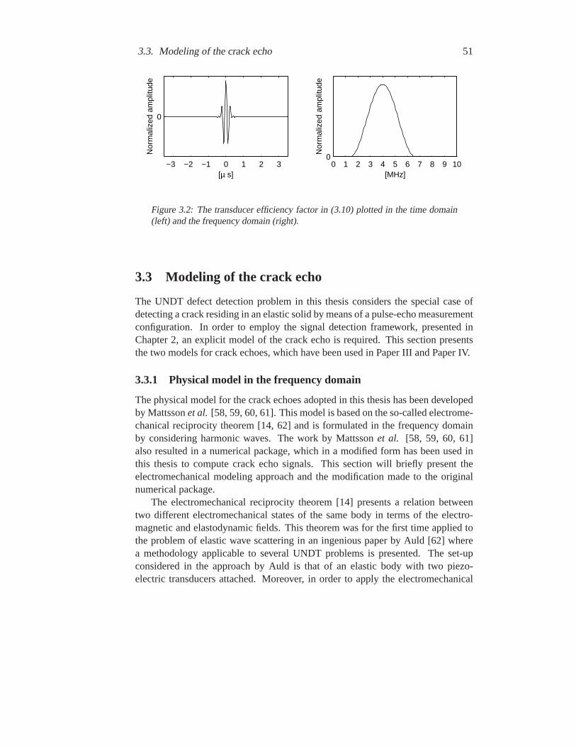
3.3. Modeling of the crack echo 51
−3 −2 −1 0 1 2 3
0
[µ s]
Nor
mal
ized
am
plitu
de
0 1 2 3 4 5 6 7 8 9 100
[MHz]
Nor
mal
ized
am
plitu
de
Figure 3.2: The transducer efficiency factor in (3.10) plotted in the time domain(left) and the frequency domain (right).
3.3 Modeling of the crack echo
The UNDT defect detection problem in this thesis considers the special case ofdetecting a crack residing in an elastic solid by means of a pulse-echo measurementconfiguration. In order to employ the signal detection framework, presented inChapter 2, an explicit model of the crack echo is required. This section presentsthe two models for crack echoes, which have been used in Paper III and Paper IV.
3.3.1 Physical model in the frequency domain
The physical model for the crack echoes adopted in this thesis has been developedby Mattssonet al. [58, 59, 60, 61]. This model is based on the so-called electrome-chanical reciprocity theorem [14, 62] and is formulated in the frequency domainby considering harmonic waves. The work by Mattssonet al. [58, 59, 60, 61]also resulted in a numerical package, which in a modified form has been used inthis thesis to compute crack echo signals. This section will briefly present theelectromechanical modeling approach and the modification made to the originalnumerical package.
The electromechanical reciprocity theorem [14] presents a relation betweentwo different electromechanical states of the same body in terms of the electro-magnetic and elastodynamic fields. This theorem was for the first time applied tothe problem of elastic wave scattering in an ingenious paper by Auld [62] wherea methodology applicable to several UNDT problems is presented. The set-upconsidered in the approach by Auld is that of an elastic body with two piezo-electric transducers attached. Moreover, in order to apply the electromechanical

52 Chapter 3: Defect detection in ultrasonic nondestructive testing
reciprocity theorem the two different states of the considered volume must be de-fined. In the approach by Auld, the first state corresponds to the solution when oneof the transducers is excited by an electromagnetic wave, which carries powerPand is of frequencyω, in the absence of the defect. The second state correspondsto the solution when the other transducer is excited by an electromagnetic wavewith the same frequency and power, butin the presence of the defect. Auld derivesan expression for the reflection coefficient, at the receiving transducer, due to thescatterer. The reflection coefficient, in Cartesian tensor notation, is given by [62]
δΓ(ω) =iω
4P
∫x∈SF
[u(1)k (ω, x)τ (2)
kl (ω, x) − u(2)k (ω, x)τ (1)
kl (ω, x)]n(SF )l dx,
(3.11)where i =
√−1, P is a constant representing the feeding power to the firing
transducer,u(b)k and τ
(b)kl are the displacement and stress, respectively, andb =
1, 2 denotes the state. Moreover, the integration in (3.11) is performed overthe surface of the defect here denotedSF and n(SF ) denotes the inward-directednormal toSF . From a signal processing point of view the reflection coefficientin (3.11) is simply a frequency domain expression of the impulse response of thedefect observed at the receiving transducer.
As mentioned in the previous section, the electrical signal from the receivingtransducer generated by a defect echo is obtained by convolving the transducerefficiency factor in (3.9) with the impulse response of the defect. In the frequencydomain this operation corresponds to a multiplication. Thus, the electrical signalin the frequency domain can be expressed as
s(ω) = β(ω)δΓ(ω). (3.12)
For the pulse echo set-up considered in this thesis there is only one transducerpresent but the approach by Auld is still applicable by simply letting the positionfor the two transducers coincide. The problem geometry as well as the crack spe-cific parameters are depicted in Figure 3.3. The crack defect is modeled as openand strip-like with an infinite length in theY -direction. Moreover, the boundaryconditions at the crack, expressed in the primed coordinate system in Figure 3.3,are taken to be so-called spring boundary conditions [61]
uk(x′, y′, 0+) − uk(x′, y′, 0−) = 0, |x′| > w/2, ∀y′
Kkl[ul(x′, y′, 0+) − ul(x′, y′, 0−)] = w n(z′)l τlk(x′, y′, 0−), |x′| ≤ w/2, ∀y′
n(z′)l τlk(x′, y′, 0+) − n
(z′)l τlk(x′, y′, 0−) = 0, ∀x′, ∀y′.
(3.13)
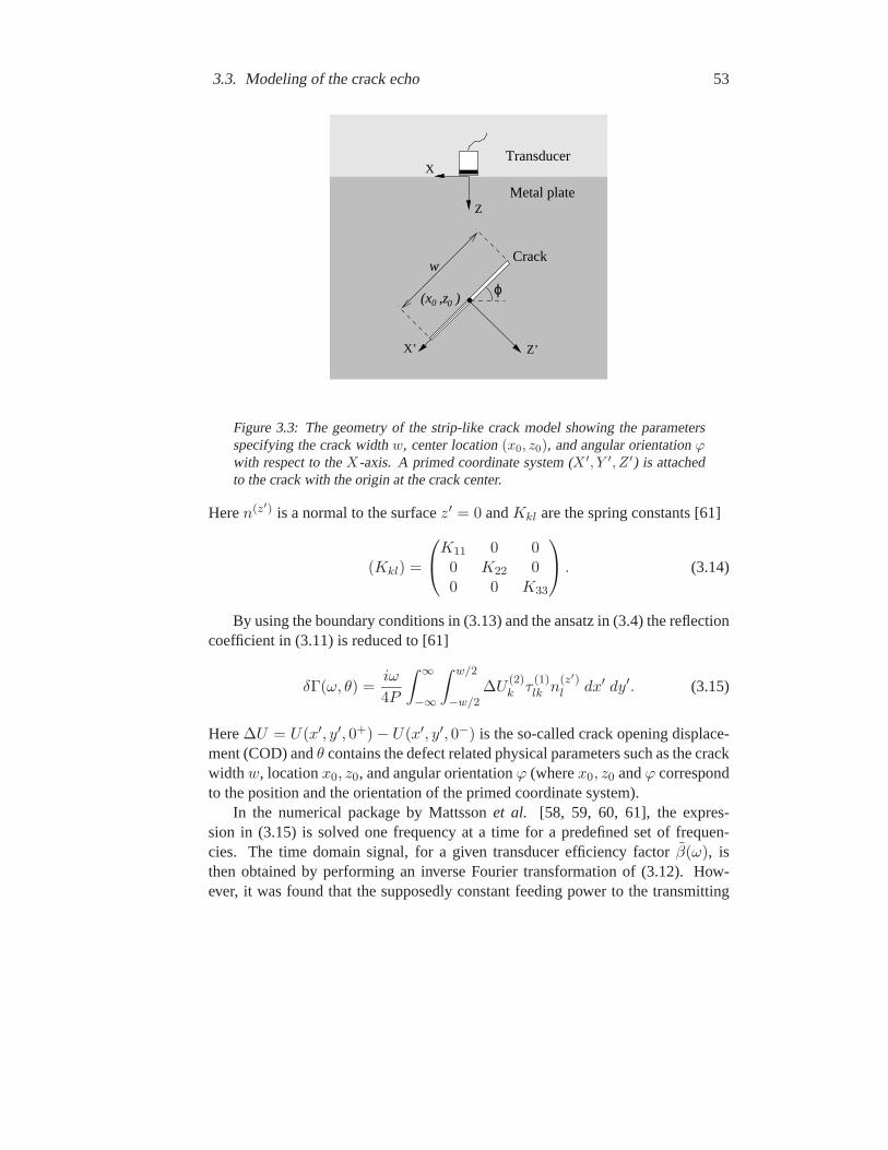
3.3. Modeling of the crack echo 53
X
Z
X’ Z’
0 0(x ,z )
Transducer
ϕ
w
Metal plate
Crack
Figure 3.3: The geometry of the strip-like crack model showing the parametersspecifying the crack widthw, center location(x0, z0), and angular orientationϕwith respect to theX-axis. A primed coordinate system (X ′, Y ′, Z ′) is attachedto the crack with the origin at the crack center.
Heren(z′) is a normal to the surfacez′ = 0 andKkl are the spring constants [61]
(Kkl) =
K11 0 0
0 K22 00 0 K33
. (3.14)
By using the boundary conditions in (3.13) and the ansatz in (3.4) the reflectioncoefficient in (3.11) is reduced to [61]
δΓ(ω, θ) =iω
4P
∫ ∞
−∞
∫ w/2
−w/2∆U
(2)k τ
(1)lk n
(z′)l dx′ dy′. (3.15)
Here∆U = U(x′, y′, 0+) − U(x′, y′, 0−) is the so-called crack opening displace-ment (COD) andθ contains the defect related physical parameters such as the crackwidth w, locationx0, z0, and angular orientationϕ (wherex0, z0 andϕ correspondto the position and the orientation of the primed coordinate system).
In the numerical package by Mattssonet al. [58, 59, 60, 61], the expres-sion in (3.15) is solved one frequency at a time for a predefined set of frequen-cies. The time domain signal, for a given transducer efficiency factorβ(ω), isthen obtained by performing an inverse Fourier transformation of (3.12). How-ever, it was found that the supposedly constant feeding power to the transmitting

54 Chapter 3: Defect detection in ultrasonic nondestructive testing
probe, i.e.P in (3.15), was indirectly varied as a function of frequency in the orig-inal numerical package. Instead of assigning a specific feeding power,P , to thetransmitting transducer a constant displacement amplitude,U0, is assigned at thesurface,ST , of the transducer. Since the displacement is uniform over the face ofthe transducer it is acting as a piston source. The feeding power to a piston trans-ducer that is required to maintain a displacement amplitude,U0, independent of thedisplacement frequency,ω, is proportional to [14]
P ∝ cρω2U20 , (3.16)
wherec is the sound velocity andρ is the density of the wave propagation medium.Thus, from (3.16) it is clear that assigning a constant displacement amplitudeU0
implies a feeding powerP that increases withω2. This behavior results in crackecho signals that are significantly up-shifted in frequency, see right column in Fig-ure 3.4 were signals corresponding to a crack with different angular orientationsare displayed. The original computer package was therefore modified by introduc-ing a frequency scaling of the assigned displacement amplitude for the transmittingtransducer according to
U0(ω) ∝ 1ω
√P
cρ, ω = 0, (3.17)
whereP is kept constant.Simulated crack echo signals with the constant feeding power modification are
presented in the left column in Figure 3.4. These echo signals are computed fora strip-like crack with different angular orientationsϕ (see Figure 3.3) and with aprobe efficiency factor given by (3.10). From Figure 3.4 it can clearly be seen thatthe echo from a crack withϕ = 45o andϕ = 90o contains several pulses. The firstand the second pulses are reflections of the P-wave from the cracks near-tip andfar-tip, respectively. The other pulses, which arrives later in time, are due to theslower propagating mode converted waves [58].
3.3.2 Phenomenological model in the time domain
In the previous section the physical principles governing elastodynamic wave mo-tions were utilized to obtain an advanced numerical model of the crack echo. Inthis section the crack echo is represented by a simple phenomenological modelin the form of an explicit mathematical expression based on qualitative reasoningof the involved scattering mechanisms. This model is employed in Paper IV, andis inspired by the impulse-response method by Lhemery, who has published a se-ries of theoretical and application oriented papers on the subject [63, 64, 65, 66].

3.3. Modeling of the crack echo 55
27 28 29 30 31 32 33 34−1
−0.5
0
0.5
1(a)
Nor
mal
ized
ampl
itude
27 28 29 30 31 32 33 34−1
−0.5
0
0.5
1(d)
27 28 29 30 31 32 33 34−0.04
−0.02
0
0.02
0.04(b)
Nor
mal
ized
ampl
itude
27 28 29 30 31 32 33 34−0.04
−0.02
0
0.02
0.04(e)
27 28 29 30 31 32 33 34−0.02
−0.01
0
0.01
0.02(c)
t [µ s]
Nor
mal
ized
ampl
itude
27 28 29 30 31 32 33 34−0.02
−0.01
0
0.01
0.02(f)
t [µ s]
Figure 3.4: Crack echoes for different angular orientationsϕ = 0 (upper row),ϕ = 45o(middle row) andϕ = 90o(last row), computed with the original numeri-cal package (d)-(f) and the modified version (a)-(c).
Although the impulse-response method is also based on fundamental physical prin-ciples its formulation allows approximations to easily be introduced. This is a greatadvantage since, apart from the obvious desire that the model should represent thecrack echo accurately, another main objective is that the model is tractable for de-riving detectors.
The impulse-response method is formulated in the time domain, in contrast tothe modeling approach in the previous section. A defect echo signal can therebybe expressed as [63]
s(t; θ) = β(t) ∗ h(t; θ), (3.18)
whereβ(t) is the transducer efficiency,h(t; θ) is the impulse response of the de-fect andθ, as before, represents the underlying physical parameters such as shape,location, orientation etc. A general approach to derive the impulse response for adefect of complex geometry and with different acoustical impedances can be foundin [66].
56 Chapter 3: Defect detection in ultrasonic nondestructive testing
In [65] Lhemery studies the special case of a so-called penny shaped crackand presents a signal processing method for defect discrimination. Lhemery showsthat the impulse response for a penny shaped crack consist of two componentsseparated in time. The one appearing first in time is the contribution from thecrack tip closest to the receiving transducer and the second is from the far tip. Thecrack defect impulse response can then be described by
h(t; θ) = hnear tip(t; θ) + hfar tip(t; θ). (3.19)
The occurrence of separate signal components, indicated by (3.19), can alsobe observed in the simulated crack echo responses in Figure 3.4, where also afew more mode converted pulses appears. Based on these simple observations theexpression in (3.19) is extended to includeM components. This yields
h(t; θ) =M∑
m=1
hm(t; θ), (3.20)
whereh1(t; θ) andh2(t; θ) are the near-tip and far-tip impulse responses respec-tively. The remaining terms in (3.20) represent the mode converted contributionsin the crack impulse response.
Instead of deriving a physically based expression for eachhm(t; θ) in (3.20)according to [66] a simple parametric model is postulated. Since the transduceris assumed to generate a transient wave-pulse the efficiency factorβ(t) will havea bandpass character. Thus, each signal component consisting ofβ(t) ∗ hm(t; θ)will also be bandpass and can thereby be represented by an amplitude modulatedsinusoid [13]
β(t) ∗ hm(t; θ) ≈
Amam(t − τm) sin(ωm(t − τm) + φm), t ∈ [τm, τm + Ta]0, otherwise
θm = [Am ωm τm φm].(3.21)
Hereτm is the arrival time,Am is the amplitude,ωm is the carrier frequency,φm isthe phase angle,am(t) is the envelope andTa is the time duration of the envelope.The phenomenological crack scattering model then becomes
s(t; θ) ≈ s(t; θ1, . . . , θM , a1, . . . , aM ) =M∑
m=1
x[t; θm, am(t)], (3.22)
wherex[t; θm, am(t)] is given by (3.21). Note that the physical parameterθ hasbeen replaced by a set of “unphysical” parameters,θ1, . . . , θM , and the envelopesa1(t), . . . , aM (t).

3.4. Modeling of clutter noise in metals 57
3.4 Modeling of clutter noise in metals
Polycrystalline materials, such as stainless steel and copper, consist of denselypacked crystals or grains, which are randomly configured throughout the material.Therefore, in an UNDT scenario, when an acoustic pulse is emitted into a materialthe pulse will be scattered by a myriad of micro-structures causing the receivedsignal to exhibit a random behavior. This signal is commonly called clutter.
It has been shown that the clutter signal from materials can be modeled as acolored Gaussian process when the number of grains is large [46, 47]. Due to thisproperty, clutter models in UNDT studies are often modeled as colored Gaussianprocesses [26, 49, 50, 67]. One evident dilemma with this approach is to find outhow the noise process should be colored. An approach to overcome this difficulty isto derive a physical model based on the material micro-structural properties. Sucha clutter model has been put forward by Yaldaet al. [38] and Margetanet al. [68].
The clutter noise model used in this thesis (Paper III and Paper IV), is a mod-ification of the model by Yaldaet al. [38], which considers an immersion testingpule-echo set-up with a focused transducer. The new model, derived in Paper IIIand briefly presented here, is modified in the following aspects:
• The configuration is that of pulse-echo contact testing.
• The transducer is modeled as unfocused.
• Approximations are introduced to reduce the computational complexity.
The backscattered noise is assumed to be dominated by single scattering of theincident wave field by the individual grains. Based on this assumption the basicidea in this modeling approach is that the clutter noise is a superposition of thebackscattered field from all grains isonified by the transmitting transducer.
By specifying the time interval within which the clutter noise signal is to becomputed will impose restrictions on the depth coordinate. Thistime window ofinterest (TWOI) together with the beam pattern for the transducer yields aspatialregion of interest (SROI) within which the backscattering from grains are to bemodeled. The geometry of the problem is depicted in Figure 3.5.
In the model by Yaldaet al. [38] a clutter noise realization is obtained byadding the backscattered field from all grains in the SROI. To alleviate much of thecomputational complexity the SROI is here first decomposed intoN sub-regionsSROIn, which are slices perpendicular to the propagation direction of the incidentwave, see Figure 3.5. The backscattered contribution from all grains within theSROIn can then be represented by a frequency and depth dependent random vari-ableQn(ω). The statistical properties ofQn(ω) are derived in Paper III, where it

58 Chapter 3: Defect detection in ultrasonic nondestructive testing
SROI
SROIn φl
∆dlx
l th Grain:33(C )lρlrl
X
Z
, ,
Amplification ofmaterial grains
Metal plate
Transducer
Figure 3.5: Sketch over the clutter noise model geometry illustrating the SROI andthel:th grain residing in then:th sub region, SROIn.
is shown, based on the central limit theorem, thatQn(ω) can be modeled as a zeromean Gaussian random variable. The frequency domain clutter noise signal can beexpressed as
v(ω) = β(ω)ω2
4πρc4
N∑n=1
exp2(j ωc − α)RnRn
Qn(ω), (3.23)
whereα is the material attenuation coefficient,Rn is the distance from the trans-ducer to the center of then:th slice.
The discrete time clutter noise realizations used in Paper III and Paper IVwere computed by a numerical implementation of (3.23) under the assumptionof a large number of grains. In this implementation a clutter noise realization,v = [v(1), . . . , v(N)]T , is obtained by an inverse discrete Fourier transformationof [v(ω1), . . . , v(ωN )] computed from (3.23) atN equidistant frequencies. Sincethe frequency domain clutter signal in (3.23) consists of linear combinations ofGaussian random variables, its inverse Fourier transform,v, will also be Gaussian.
A realization of a typical clutter noise signal for a stainless steel with a probeefficiency factor given by (3.10) is depicted in Figure 3.6 in both the time and thefrequency domain.

3.5. Signal detection applied to nondestructive testing 59
27 28 29 30 31 32 33 34
0
[µ s]
Nor
mal
ized
am
plitu
de
0 1 2 3 4 5 6 7 8 9 100
[MHz]
Nor
mal
ized
am
plitu
de
Figure 3.6: A clutter noise realization in the time domain (left) and the corre-sponding discrete Fourier transform (right).
3.5 Signal detection applied to nondestructive testing
The framework of parameterized signal detection, presented in Section 2.1.2, issuitable for treating the defect detection problem. In a typical UNDT situation, apotential defect can have different locations, orientations, and shapes, all of whichwill affect the backscattered wave-field and thereby the measured signal. Thesedefect related physical attributes, which for example are represented byθ in (3.15),can often be considered a priori unknown from one inspection to another. Theuncertainty about the defect related physical attributes can be modeled by con-sideringθ to be a realization of a stochastic variableΘ with the pdfpΘ. Thus,the uncertainty aboutθ is transformed into an uncertainty about the defect echos. The ensemble of the defect echo signals for all possible values ofθ may berepresented by
S = s(θ) ∈ RN | θ ∈ Λ, (3.24)
whereΛ is the set whereθ takes its values.In a testing situation the defect echo,s(θ), is drawn from the signal familyS
in (3.24), according to the pdfpΘ(θ). Moreover, by omitting multiple reflectionsthe clutter noise can be considered both as additive and independent of the defectgenerated signal. Thus, the defect detection problem can be cast as the compositehypothesis test
H0 : Y = VH1 : Y = s(Θ) + V ,
(3.25)
whereV ∼ N (0, ΣV ) represents the clutter noise.

60 Chapter 3: Defect detection in ultrasonic nondestructive testing
As shown in Section 2.1.2, a decision rule for (3.25) can be formulated as
δ(y) =
1 if T (y) ≥ τ
0 if T (y) < τ.(3.26)
Hereτ is a user defined threshold andT is a detection statistic given by either thelikelihood ratio in (2.23), for the NP and Bayes optimal detector, or the maximumlikelihood ratio in (2.24) for the generalized likelihood ratio test (GLRT).
The particular problem considered in Paper III and Paper IV is to detect a strip-like crack residing in an elastic solid. Equipped with the signal models presentedin Sections 3.3.1 and 3.3.2 a few approaches to compute a detection statistic arepresented in the following sections.
3.5.1 Physical model based crack echo detector
Instead of pursuing an analytical approach in deriving a detector for strip-likecracks, the likelihood ratio in (2.23) can be computed numerically. This is sim-ply achieved by a discretization of the pdfpΘ in (2.23) atM sample pointsθm,and generatings(θm) by means of the computerized mathematical model of thecrack scattering described in Section 3.3.1. Thus, the numerical approximation ofthe likelihood ratio reads
L(y) =∫
θ∈ΛL(y|θ) pΘ(θ) dθ ≈
M∑m=1
L(y|θm) Pθm , (3.27)
wherePθm = pθ(θm)∆θ and∆θ is the volume around each sampling point. Theconditional likelihood ratio in (3.27) is
L(y|θm) = exp
s(θm)T Σ−1V y − 1
2s(θm)T Σ−1
V s(θm)
. (3.28)
The NP and Bayes optimal detector for (3.25) can be implemented as a non-linear filter bank based on (3.28) and (3.27), which is depicted in Figure 3.7 as ablock diagram.
If the a priori pdfpΘ is not known, which is often the case in a practical situa-tion, the GLRT approach can be adopted. A numerical approximation of the GLRTdetector in (2.24) can straightforwardly be obtained based on the same filter bank,given by (3.28), that was used for the NP and Bayes optimal detector. Thus, theGLRT detection statistic is
T (y) = maxm
L(y|θm). (3.29)
The corresponding block diagram for the GLRT detector is depicted in Figure 3.8.

3.5. Signal detection applied to nondestructive testing 61
ΣH
H
M
.
.
.
y y
1
0τ<>
θ2
θ
θ1
θ1L( )
L( )θ2
L( )θM
. .
.
P
P
P
L( )
Figure 3.7: Block diagram of the NP and Bayes optimal detector
H
H
.
.
.
. .
.y ymax .
1
0
θ1L( )
L( )θ2
L( )θM
>τ<T( )
Figure 3.8: Block diagram of the GLRT detector
In Paper III the detection approaches described above are exemplified by as-suming that the cracks position(x0, z0), widthw, and the constantsKij are knownwhile the angular orientationϕ is unknown, see Figure 3.3 and the boundary condi-tions in (3.13). Thus, in this caseθ in (3.28) and (3.29) corresponds to the angularorientationϕ of the crack. One should note that a fundamental limitation of thefilter bank implementation of the detectors described above is the computationalcomplexity. For a problem withK unknown parameters which need to be dis-cretized intoM different intervals, the number of filters in the filter bank isMK ,i.e. the number of filters grows exponentially with the number of parametersK.Thus, except for problems with few unknown parameters, one has to consider sub-optimal family detectors with lower complexity.

62 Chapter 3: Defect detection in ultrasonic nondestructive testing
3.5.2 Phenomenological model based crack echo detector
The phenomenological signal model in Section 3.3.2 has been employed in Pa-per IV to obtain low complexity detectors for crack defects. This signal modelconsists of superpositions of pulses given by (3.21). Since the statistical variabil-ity of the underlying physical parameters of the cracks were represented by thestochastic variableΘ in (3.25), the arrival time and waveform parameters in (3.21)are also modeled as stochastic. The problem of detecting several pulses with un-known arrival time is studied in Paper II, where an approximation of the NP andBayes optimal detection statistic is given. This result is applied in Paper IV to thecrack echo detection problem. In order to obtain a simple detection statistic, of lowcomputational complexity, the following assumptions are imposed:
• The number of pulses are assumed to be fixed and the stochastic parametersof the pulses are assumed to be statistically independent.
• The carrier frequencies are assumed to be equal and deterministic but un-known for all pulses and will be denotedωc.
• The discrete time envelopes for all pulses are assumed to be known and equaland denoteda = [a(1), . . . , a(Na)]T , whereNa is the number of samples ofthe envelope.
• The arrival timesτ1, . . . , τM are assumed to be realizations from indepen-dent identically distributed (i.i.d.) stochastic variables with a uniform dis-tribution on the observation interval. In the discrete time representation thiscorresponds to a uniform probability mass function on[1, N − Na].
• The pulse durations are assumed to be short relative the acquisition time, i.e.Na N .
Under these assumptions the detection statistic takes the form (see Paper II)
T (y) =N−Na∑n=1
EA,φ
Lωc(y
n+Nan |A, φ)
, (3.30)
whereyn+Nan denotes the sub-vector ofy from n to n + Na and
Lωc(yn+Nan |A, φ) = exp
xT Σ−1
V yn+Nan − 1
2xT Σ−1
V x
. (3.31)
HereΣV is the covariance matrix (of sizeNa × Na) of the noiseV and
x(n; A, φ, ωc) = Aa(n) sin(ωc(n − 1)Ts + φ) n = 1, . . . , Na, (3.32)
whereTs is the sampling time.

3.5. Signal detection applied to nondestructive testing 63
The assumptions listed above are not based on any detailed analysis of thestatistical properties of the model parameters but rather imposed to obtain a math-ematically tractable problem. Clearly, the position, orientation, and size of a crackwill affect the arrival times as well as the waveforms of the pulses via the intri-cate relationship between the underlying physical parameters and the parametersin (3.21). Due to the lack of knowledge concerning this intricate relationship andthe statistical properties of a potential crack’s physical parameters the assumptionslisted above are intentionally conservative in the sense that they introduce verylittle a priori knowledge. By refining these assumptions to agree more with theunderlying physical reality the detector will yield higher performance but becomesignificantly more complex. In the following subsections three approaches to solveEA,φLωc(yn+Na
n |A, φ) in (3.30) are pursued based on different assumptions ofthe statistical properties of the model parametersA andφ.
Case 1: Matched filter detector
By ignoring thatA andφ can exhibit any form of variability the problem reducesto detecting a deterministic pulse. This is equivalent to the coherent detectionproblem described in Section 2.1.1, with the likelihood ratio given by (2.8). Thus,under these simplified assumptionsEA,φLωc(yn+Na
n |A, φ) reduces to
Lλ(yn+Nan ) = exp
xT (λ)Σ−1
V yn+Nan − 1
2xT (λ)Σ−1
V x(λ)
, (3.33)
whereλ = [ωc A φ] are some fixed parameters.
Case 2: Noncoherent detector
The previous case is here extended by allowing the phaseφ to have a uniformdistribution, i.e. φ ∼ U [0, 2π]. This corresponds to the noncoherent detectionproblem, presented in Example 2.1, where the likelihood ratio is given by (2.34).Thus,EA,φLωc(yn+Na
n |A, φ) can then be expressed as
Lλ(yn+Nan ) = exp−1
4aT Σ−1
v aI0
(√(hT
s (λ)yn+Nan )2 + (hT
s (λ)yn+Nan )2
),
(3.34)wherehs(λ) andhc(λ) are given by (2.29) and depend onλ = [ωc A]. Recall thatthe likelihood ratio for the noncoherent detection problem was derived under thenarrowband approximation. Since the defect echo pulses are relatively widebandit is questionable if the narrowband approximation is satisfied for these types ofpulses.
64 Chapter 3: Defect detection in ultrasonic nondestructive testing
Case 3: Wideband quadrature matched filter detector
The final case that has been considered is when both the pulse amplitudeA andthe phaseφ are modeled as random. The amplitude is here assumed be Rayleighdistributed, i.e.A ∼ R(σA), with an unknown density parameterσA. As in the pre-vious case, the phase is taken to be uniformly distributed. This is equivalent to thedetection problem described in Example 2.2. The likelihood ratio for this problemis given in (2.47), which yields thatEA,φLωc(yn+Na
n |A, φ) can be expressed as
Lλ(yn+Nan ) = expGλ
× exp
σ2A
2(yn+Na
n )T HλHTλ yn+Na
n − σ2A
2(yn+Na
n )T HλQλHTλ yn+Na
n
,
(3.35)
whereλ = [ωc σA], andGλ, Qλ, andHλ now depend onλ and are given by (2.45),(2.48), and (2.49), respectively.
The remaining problem is now to find appropriate values for the parameterλ in(3.33), (3.34), and (3.35). As mentioned, in previous UNDT studies [28, 29, 30],parametric detectors for defects have been optimized by using the SNRE in (1.7) asa criterion function. An alternative strategy is adopted here, which is simply basedon finding the parameterλ∗ that minimizes the probability of error
λ∗ = arg minλ
PE(δλ). (3.36)
Hereδλ∗ is on the form (3.26) with the detection statistic given by (3.30).In Paper IV, the probability of error, for the three detectors presented above, is
computed versus the various parameters inλ. From these simulations it can be con-cluded that it is feasible to optimize the detector parameters based on the minimumprobability of error criterion even for quite small training data sets. Moreover, theseresults show that the detection performance is mainly dependent on the parameterspecifying the carrier frequencyωc. Also presented in Paper IV are the ROCs forthe proposed detectors, which are compared to the physical model-based optimaldetector (Paper III). Moreover, since the wideband quadrature matched filter de-tector (Case 3 above) only shows a slight improvement in the ROCs compared tothe noncoherent detector (Case 2 above) the crack echo pulses can be consideredto satisfy the narrowband condition in this context. This is supported by the studyin Paper I, where the effect of the signal bandwidth on the performance of thenoncoherent detector is analyzed. However, even though the proposed detectorsare based on quite ad hoc assumptions they result in only moderate performancedegradation compared to the physical model-based optimal detector.

Chapter 4Detectors in nonlinear sensorsystems
THIS chapter is devoted to the problem of detecting signals acquired with anonlinear sensor, for which three main topics are considered. The first is to
derive an optimal detector for a static nonlinear sensor system and in particularto evaluate the detection performance as a function of the noise strength. Thisproblem can be treated by means of the framework of non-Gaussian signal detec-tion, presented in Section 2.4. As was pointed out in Section 1.2.2, detectability innonlinear sensor systems could under certain circumstances be enhanced by noise.This phenomenon has been studied under the name of stochastic resonance (SR)[18, 19, 20, 21], which was illustrated in Example 1.1 by means of a dynamicalsystem with a harmonic input signal. The SR phenomenon has also been studiedin static (non-dynamical) systems [69, 70]. The second main topic is to proposea generally applicable quantifier for the SR phenomenon, which truly reflects theinformation processing capability of a system. The third topic concerns optimiza-tion of a tunable nonlinear sensor for detection, which is treated by employing theinsights from the two above mentioned topics.
The nonlinear sensors that have been used in this thesis are the static SQUIDand the static MR sensor, which are described in Sections 5.1 and 5.2, respectively.These sensors are used to illustrate the approaches taken for the three topics men-tioned above, which are briefly outlined in Section 5.3.
65

66 Chapter 4: Detectors in nonlinear sensor systems
4.1 The superconducting quantum interference device
The superconducting quantum interference device (SQUID) is an electromagneticapparatus that converts magnetic flux variations into a voltage variation. TheSQUID is the most sensitive magnetic sensor currently available, achieving a mag-netic field resolution in the order of10−15 Tesla. A significant limitation of thepractical usefulness of the SQUIDs is their sensitivity to both inherent and externalnoise. There are two main types of SQUIDs namely the rf (or AC) SQUID andthe DC SQUID. The rf SQUID is the one studied in Paper V, and its fundamentalcomponents are depicted in Figure 4.1. This section will only give a brief descrip-tion of the SQUID sensor, an in depth presentation of SQUIDs, their underlyingphysical mechanisms and operation can be found in [31].
Josephson junction
Superconducting ring
Low−temperature cage
eΦ
Φ
Figure 4.1: Simplified schematic of a SQUID sensor depicting the externally ap-plied magnetic fluxΦe and the fluxΦ trapped in the superconductive ring.
A time varying external magnetic flux,Φe(t), is applied to the SQUID’s super-conductive ring, which is shielded by a low-temperature cage, see Figure 4.1. Thisexternal flux is here given by
Φe(t) = Φi(t) + ΦDC + σΦV (t), (4.1)
whereΦi(t) is the input flux to be measured (detected),ΦDC is a known DC levelapplied to obtain a symmetric transfer characteristic,ΦV (t) is a noise disturbanceof zero mean and unit variance, andσ is a noise strength parameter. The noise termσΦV (t) in (4.1) can often be modeled as Gaussian with a normalized autocorrela-tion given by
R(τ) =1σ2
EtσΦV (t)σΦV (t + τ) = e−|τ |/τv , (4.2)

4.1. The superconducting quantum interference device 67
whereτv is the noise correlation time. Furthermore, the noise bandwidthτ−1v is in
many situations considerably larger than the bandwidth of input flux signalΦi(t),yielding that the noise can be approximated as being white [19].
The externally applied flux,Φe, yields a magnetic flux through the supercon-ductive loop (denotedΦ in Figure 4.1), which evolves according to the dynamicsdetermined by the superconductive properties of the ring and the Josephson junc-tion. The dynamics of the magnetic flux through the superconducting loop can bedescribed by [18, 19]
LCd2
dt2x(t) = −τL
d
dtx(t) − U ′[x(t)] + xe(t). (4.3)
Herex(t) = Φ(t)/Φ0 is the normalized flux in the loop,xe(t) = Φe(t)/Φ0 isthe normalized external flux,Φ0 = /2e is the flux quantum,L is the inductanceof the loop,C is the junction capacitance, andτL = L/Rj , whereRj is the so-called normal state resistance of the junction. Moreover,U ′(x) = d
dxU(x), withthe functionU given by [18, 19]
U(x) =12x2 − β
4π2cos(2πx), (4.4)
whereβ = 2πLIc/Φ0, andIc is the so-called loop critical current. The parameterβ determines the shape of the potential governing the dynamics of the SQUID.
In most practical applications the SQUID loop is shunted by a low resistanceyielding thatLC τL and thereby that the L.H.S. of (4.3) can be neglected [19].Thus, in these cases the dynamics in (4.3) is reduced to
τLd
dtx(t) = −U ′[x(t)] + xe(t). (4.5)
Due to the modeling assumptions above the first order system in (4.5) bears a clearresemblance to the system studied in Example 1.1 (Chapter 1) with the exceptionof being multi-well. Several studies of various SR phenomenas in rf SQUIDs de-scribed by (4.5) have been published, many of which are devoted to signal detection[15, 16, 19, 20, 21].
A further simplification of the rf SQUID transfer characteristic in (4.5) can bemade if the noise bandwidth,τ−1
v , not only is considered to be much larger than thebandwidth of the input flux signalxi(t), but also much less thanτ−1
L , i.e. τv τL.This is valid in many situations sinceτL is typically in the order of10−10 to 10−12
seconds which far exceeds the bandwidth of most real-world signals of interest.Thus, by settingτL
ddtx(t) = 0 the dynamics in (4.5) can be approximated by the
quasi-static form [71]U ′[x(t)] = xe(t). (4.6)

68 Chapter 4: Detectors in nonlinear sensor systems
The measured output voltage signal from the quasi-static rf SQUID is proportionalto the so-called shielding fluxxs(t) = x(t) − xe(t). A non-dynamic transfercharacteristic can now be obtained by solving (4.6) forxs(t) as a function ofxi(t).This has been done analytically [71, 72], in form of a Fourier-Bessel expansionwhen0 ≤ β < 1, yielding
xs(t) = limN→∞
N∑n=1
(−1)n
nπJn(nβ) sin[2πn(xi(t) + xDC)], (4.7)
wherexDC = ΦDC/Φ0 andJn denotes ann:th order Bessel function of the firstkind. The quasi-static SQUID model in (4.7) has been reported [72] to exhibitSR like phenomenon, when altering the parameterβ. However, in [72] no SNRenhancement was found when altering the noise strength parameterσ. This modelis also used in Paper V to exemplify the proposed information theoretic approachto quantify SR.
4.2 The magneto-resistive sensor
The magneto-resistive (MR) sensor utilizes the magneto-resistive effect in fer-romagnetic transition metals in order to measure external magnetic fields. Theessence of this effect is that the resistance in a ferromagnetic material is dependenton the angle between the internal magnetization and the direction of an appliedcurrent. When an external magnetic field is applied the internal magnetization isrotated, thereby changing the resistance. In Paper VI a so-called barber pole MRsensor is used to detect weak magnetic DC fields in a strong noisy background.In this work the transfer characteristic of the MR sensor is obtained experimen-tally due to difficulties to determine all the required physical parameters and alsosince the available mathematical models for MR sensors transfer characteristics arequite crude. The experimental procedure for acquiring the transfer characteristic issimply to apply external fields of known amplitude to the sensor and measure thesensors response. This section gives a brief presentation of the basic functionalityof an MR sensor, a thorough description of the MR effect can be found in [31].
The basic element in an MR sensor is a thin film of a magneto-resistive alloyetched into a rectangular shape with electrodes attached at both ends. In order tolinearize the sensor for small external fields so-called barber poles are etched onthe thin film, see Figure 4.2. The barber poles are a series of strips of high electricalconductivity that force the current flow in the thin film into a direction determinedby the inclination of the barber poles.
In ferromagnetic materials there are certain preferred directions for the mag-netization, this is due to the materials crystal structure and orientations. The most

4.2. The magneto-resistive sensor 69
y
x (e.a.)
Electricalconnector
Barberpoles
Thin filmmagnetic alloy
Mϕ
θα
I
H
I
Figure 4.2: Schematic of an MR sensor with barber poles.
preferred direction is the so-called easy axis (e.a.), which in Figure 4.2 is assumedto be aligned with thex-direction. It has been shown that the resistance of the MRelement can be described by [31]
R(θ) = R⊥ + ∆R cos2(θ). (4.8)
Hereθ is the angle between the internal magnetization,M , and the direction of theapplied current,∆R = R‖−R⊥, whereR⊥ andR‖ are the resistances perpendicu-lar and parallel, respectively, to thex-direction. Under the influence of an externalmagnetic field,H = [Hx Hy]T , the direction of the magnetizationM will rotate,which is represented by the angleϕ between the e.a. andM . An approximaterelation between the external fieldH andϕ for an ellipsoidal-shaped thin film isgiven by [31]
sin(ϕ) =Hy
H0 + Hx/ cos(ϕ), (4.9)
whereH0 is the so-called characteristic field which is material dependent. Fol-lowing [31], rough approximations of MR sensors’ transfer characteristics can beexpressed in terms of the resistance by using (4.8) and (4.9), and assuming that thex-component of the external field isHx = 0. They-component of the externalfield is here assumed to be given by
Hy(t) = Hs(t) + σHV (t), (4.10)

70 Chapter 4: Detectors in nonlinear sensor systems
whereHs(t) is the magnetic field to be measured (detected),HV (t) is an ambientzero mean unit variance white Gaussian noise disturbance, andσ is a noise strengthparameter.
For an elliptic MR element without barber polesα ≈ 0, which yields thatθ ≈ ϕ (see Figure 4.2). Thus, by using (4.8) and (4.9) the resistance can beexpressed as a function of they-component of the external field according to
R(Hy) = R0 − ∆R
(Hy
H0
)2
, (4.11)
whereR0 = R⊥ + ∆R. Figure 4.3 depicts the resistanceR as a function of theexternal filedHy normalized byH0.
The resistance for an elliptic MR element with barber poles, inclined so thatα = 45o, can be expressed as [31]
R(Hy) = R0 − ∆RHy
H0
√1 −
(Hy
H0
)2
. (4.12)
A typical behavior of the transfer characteristic in (4.12) is depicted in Figure 4.3,where it can clearly be seen thatR(Hy) can be well approximated as linear forHy/H0 close to zero. However, if the sensor is intended to operate in a very noisyenvironment then the external field can not be confined to small amplitudes only,thereby violating the classical operating conditions. In these situations a widerdomain of the MR sensor transfer characteristic will be utilized yielding that thesensor must be considered both nonlinear and non-bijective.
−1.5 −1 −0.5 0 0.5 1 1.5H
y / H
0
R0−∆R
R0− ∆R/2
R0
Figure 4.3: Typical transfer characteristics of an MR sensor expressed in terms ofthe MR elements resistance as a function of the external fieldsy-component. Theresistance is plotted for an MR element without barber poles (dashed) and withbarber poles (solid).

4.3. Optimal detectors in static nonlinear sensor systems 71
4.3 Optimal detectors in static nonlinear sensor systems
The problem of detecting a known signal contaminated by additive noise and mea-sured by means of a static nonlinear sensor is considered. Moreover, the sensor’sstatic nonlinear transfer characteristic, below denotedg, is assumed to be knownyielding that the problem can be expressed as a binary hypothesis test on the form
H0 : Yn = g(σVn), n = 1, . . . , NH1 : Yn = g(sn + σVn), n = 1, . . . , N.
(4.13)
Here,s = [s1, . . . , sN ]T is the sampled signal to be detected,σ is a noise strengthparameter andV1, . . . , VN are noise samples, which are assumed to be i.i.d. Gaus-sian with zero mean and unit variance.
The hypotheses in (4.13) can be directly associated with those in (2.72) yield-ing an optimal detector on the from
δ(y) =
1 if L(y) ≥ τ
0 if L(y) < τ,(4.14)
where the likelihood ratio is given by
L(y) =N∏
n=1
M∑m=1
pV (c(m)yn )
|g′(sn + c(m)yn )|
/ K∑k=1
pV (b(k)yn )
|g′(b(k)yn )|
. (4.15)
In the following two sections the particular problems covered in Paper V andPaper VI, are briefly presented.
4.3.1 Detectability in nonlinear sensor systems
In this section, the performance of a sensor-detector system, in terms of detectabil-ity as a function of the noise strength, is considered. As mentioned previously,these types of studies have been conducted under the name of stochastic resonance(SR), where various kinds of SNR measures, computed on the output of the sensor,has been used to reflect the performance as a function of the noise strengthσ. Thedeflection ratio orgeneralized signal-to-noise ratio can be used to express many ofthe various definitions of SNRs by appropriately choosing1 the functionG below.The deflection ratio is defined by [8, 40]
d∆(p0, p1) (E1
G(Y )
− E0
G(Y )
)2Var0
G(Y )
, (4.16)
1For example, a connection between the deflection ratio in (4.16) and the SNR in (1.11), whichhas been used in several SR studies, is derived in [73].

72 Chapter 4: Detectors in nonlinear sensor systems
wherep0 andp1 are the pdfs ofY underH0 andH1, respectively, and Var0G(Y )denotes the variance ofG(Y ) underH0. However, unlessG in (4.16) is givenby the likelihood ratio in (4.15), the SNRs are not adequate for evaluating theperformance of a nonlinear sensor with respect to hypothesis testing (for detailssee Appendix B). In such situations alternative measures must be employed whichincorporate the whole probabilistic structure of the problem at hand.
From an information theoretic perspective, the problem of assessing perfor-mance of a signal transformation, such as performed by a sensor, can be seen asevaluating how much relevant information that is preserved after the signal hasbeen processed. The hypotheses of the underlying signal in (4.13), i.e. before theinfluence of the sensor, can be described by
H0 : Xn = σVn, n = 1, . . . , NH1 : Xn = sn + σVn, n = 1, . . . , N.
(4.17)
The ability to discriminate betweenH0 andH1 in (4.17) is determined by the pdfsof X = [X1, . . . , XN ]T underH0 and H1, which shall be denotedp0 and p1,respectively. Likewise, the ability to discriminate betweenH0 andH1 in (4.13)depends on the corresponding pdfs ofY , i.e. p0 andp1, which are determinedby g as well asp0 andp1. Moreover, the optimal performance for discriminatingbetween the hypotheses in (4.17) gives the upper limit for the hypothesis test in(4.13), which is achievable ifg in (4.13) is sufficient for the binary hypothesisproblem in (4.17), i.e. sufficient forp0, p1. A brief discussion on sufficientstatistics can be found in Appendix B.
Instead of following the conventional SR approach, by computing some kindof SNR, an alternative route is taken where the so-calledf -divergences are used tocompute a performance measure based on the pdfs of the sensor output signal. Thef -divergences are described by [39, 40, 41]
df (p0, p1) = h
(∫y∈RN
f
(p1(y)p0(y)
)p0(y) dy
), (4.18)
whereh is an increasing function onR andf is a convex2 real function onR+,i.e. [0,∞]. The properties for thef -divergences are summarized in Appendix B,where it is pointed out that these measures, in contrast to the SNRs, can be used toevaluate if a given signal transformation is sufficient with respect top0, p1.
The basic idea for evaluating the information processing capability of a sen-sor, is to computedf (p1, p0) as a function of the noise strengthσ and examine ifthe divergence exhibits a local maximum for increased noise strengthσ. It should
2A function is said to be convex if for any two pointsA andB on the curvey = f(x), the chordbetweenA andB lies above the curve.
4.3. Optimal detectors in static nonlinear sensor systems 73
be noted that the hypothesis problem in (4.17) is equivalent to the coherent detec-tion problem described in Section 2.1.1, where it is shown that the detection per-formance is monotonically dependent ond in (2.15), which for (4.17) reduces tod = sT s/σ2. This yields thatdf (p0, p1) is monotonically dependent ond, whereasthe behavior ofdf (p0, p1) not only depends ond but also ong.
For the particular problem studied in Paper V,g is the static SQUID transfercharacteristic in (4.7) and the hypotheses in (4.13) are reduced to only include asingle time sample sinces is taken to be a known DC signalµ. Moreover, the de-tection performance for the SQUID sensor-detector system is evaluated in terms ofdf (p0, p1) for increasing values of the noise strengthσ while simultaneously scal-ing the DC levelµ so thatd = µ2/σ2 is kept constant. The particularf -divergencemeasure that is used in this study is the so-called Kolmogorov variational distance3.In addition to the Kolmogorov variational distance the performance is also ex-pressed in terms ROC curves and minimum achievable probability of error for theoptimal detector in (4.14). Based on these performance measures it is shown thatthe detectability in a static SQUID sensor system can be enhanced by increasing thenoise strengthσ. However, such a noise enhanced detection performance will notoccur if g in (4.13) is bijective and the detector is optimal. As a conclusion it canbe stated that a necessary requirement for noise enhanced information processingperformance of a nonlinear system is that the system is non-bijective.
The use off -divergences as quantifier for SR, which was proposed in Paper V,are applied to a dynamical system, similar to the system in Example 1.1, in a paperby Robinsonet al. [74]. In [74] it is shown that the detectability does not exhibitenhancement when increasing the noise strength. This result is in conflict withthe generally accepted notion of SR and is simply due to the fact that the systemis bijective. It represents an interesting example of how the SNR measures, thattraditionally has been used to quantify SR, does not suffice in describing the infor-mation processing capability of a nonlinear system.
4.3.2 Sensor optimization for detection
In most practical detection scenarios the strength of the ambient noise can not bealtered, which was the case considered in the previous section. A more practicallyrelevant problem is tuning of a sensor’s transfer characteristic in order to improvethe detectability in a given measurement environment. The hypotheses for thisproblem can be expressed as
H0 : Yn = gβ(σVn), n = 1, . . . , NH1 : Yn = gβ(sn + σVn), n = 1, . . . , N.
(4.19)
3The Kolmogorov variational distance is given by (4.18) withh(z) = z andf(z) = |π1z − π0|.

74 Chapter 4: Detectors in nonlinear sensor systems
whereβ is some parameter by which the sensor transfer function may be modified.If gβ is bijective for all possible parameter settings it will clearly be sufficient
for all inference problems since the inverse,g−1β , exist for allβ. However, ifgβ is
not bijective for anyβ it is not immediately clear ifgβ is sufficient for a particularinference problem. Therefore, when facing an inference problem which is to besolved based the statisticgβ(X) the success could be crucially dependent on thechoice ofβ. This naturally leads to the problem of finding a parameter setting sothe function either becomes bijective or preserves as much relevant informationas possible concerning the particular inference problem. As mentioned earlier, inthe detection performance studies by Hibbset al. [15] and Rouseet al. [16],the sensor is tuned to operate in the SR regime where the quantifier (the tuningcriterion function) is the SNR in (1.11). Due to the weakness of the SNR measurethe approach taken here is instead based on thef -divergences as a tuning criterionfunction. Thus, the optimal setting forβ in (4.19) is given by
β∗ = arg maxβ
df (p0, p1). (4.20)
This approach simply strives to findβ that maximizes the divergence between thepdfs of the sensor output underH0 andH1, i.e. p0 andp1 respectively.
The SQUID sensor and the MR sensor, presented in the previous sections, areused in Paper V and Paper VI to illustrate the sensor tuning approach by meansof f -divergences. In these studies the objective is to operate the sensors in a noisyenvironment where it can not be guaranteed that the sensors are confined to operatein their linear regime.
In paper V, the Kolmogorov variational distance is displayed versus the staticSQUID nonlinearity parameterβ in (4.7). This result shows that, for a given noisestrengthσ, the Kolmogorov variational distance, and thereby the detectability, es-sentially increases monotonically with increasingβ.
In paper VI, a similar study based on the MR sensor is performed, where theKolmogorov variational distance and the Kullback-Leibler divergence4 are usedas optimization criteria. In this paper the sensor tuning is performed by simplyinjecting a known DC signal at the sensor input. Thus, the transfer function in(4.19) is given bygβ(X) = g(β+X), whereβ is the known DC tuning andg is theexperimentally determined transfer function, which resembles the transfer functionin (4.12). From this study it is shown that both divergence measures display distinctlocal maxima, which indicate that by properly choosingβ, the MR sensor can betuned to improve the detectability for a given measurement environment.
4The Kullback-Leibler divergence is given by (4.18) withh(z) = z andf(z) = − lnz.

Chapter 5Concluding remarks and futurework
THIS chapter will give some general comments and remarks on the insightsthat have been gained in this thesis in addition to the specific conclusions
that are presented in the papers and throughout the previous chapters. Also brieflydiscussed in this chapter are some possible directions for future work.
As mentioned in the introduction, the main objective of this thesis is to con-tribute to the engineering quest by explicitly derive and apply optimal detectors forspecial, practically relevant problems. The particular problems in focus were todetect transient signal families as well as signals acquired with nonlinear sensors.This quest lead, for example, to the study of detecting multiple pulses with un-known arrival times, which is applicable to the UNDT application, even though theunderlying assumptions may not be fully satisfied. This quest also lead to the studyof detection of wideband signals, since, for example, the pulses generated from anUNDT system can exhibit a rather wideband characteristic. However, the pulsesfrom an UNDT system will, more often than not, be narrow enough for the narrow-band approximation to hold, yielding that the classical noncoherent and quadraturematched filter detectors can not be ruled out for these types of applications. Still,the use of the analytical solutions to the wideband noncoherent and quadraturematched filter detectors might be applicable in situations where a stationary har-monic signal source is located in a Gaussian noise environment and the measuredsignal is obtained by a mobile sensor that travels by the source with a high speed.This scenario can, for example, occur in air-borne surveillance systems.
The main conclusion regarding the UNDT defect detection problem is that theframework of composite hypothesis testing is appropriate since it can treat the oc-
75

76 Chapter 5: Concluding remarks and future work
currence of defects of various shapes and orientations. Moreover, a suitable ap-proach to obtain detectors for this problem is to employ the solution techniques fordetection of parameterized signals, where the signals can be represented either bya physical model or a phenomenological model. If sufficienta priori knowledge isavailable the physically model based strategy has the benefit of being optimal andcan be used for a wide variety of defect types as long as a physical model is ac-cessible. On the other hand, the phenomenological model based approach has thebenefit of reducing the computational complexity and also that the assumptions re-garding the signal models are explicit. Thus, any reduction in performance relativeto the optimal performance can be directly traced to the imposed modeling assump-tions. Any detection approach where the modeling assumptions are implicit, suchas split spectrum processing (SSP), makes parameter tuning and interpretations ofperformance behavior less obvious.
The most urgent direction for future work is to perform real data experiments,where the proposed detector strategies can be employed and the validity of both thephysical and the phenomenological defect echo models investigated. An obstaclein such a study, which is of significant importance, is to find a practically realizableapproach to estimate detector performance, for example in the form of ROC curves.Another important direction for future work is to extend the statistical hypothesistesting problem to include multidimensional signals, acquired e.g. with a sensorarray.
Throughout the thesis, and in most practical applications, the ultrasonic exci-tation pulse has beena priori determined without a detailed consideration to theparticular detection problem at hand. An interesting aspect of pulse-echo detectionproblems, not only applicable to UNDT but also to sonar and radar, is to determinethe most appropriate pulse to transmit in order to maximize detectability.
The framework of optimal signal detection is also suitable for detection prob-lems when the signals are acquired with nonlinear sensors. However, this prob-lem departs from the analytically tractable case of Gaussian signal detection andthereby requires either more advanced analytical treatment or retreating to numer-ical solution techniques. The main conclusion for the nonlinear sensor-detectorapplication is that the stochastic resonance (SR) phenomenons can be treated byutilizing concepts from both optimal signal detection and information theory. Inparticular, by quantifying the SR effect in terms of thef -divergences yields thatthe phenomenon can truly be interpreted as a noise enhanced gain of the systemsinformation throughput. Apart from detection, another interesting problem is sig-nal/parameter estimation in nonlinear sensor systems.

Appendix ABackground on binary hypothesistesting
In this Appendix the binary hypothesis testing problem is treated in some moredetail to give the reader additional insight into the role of the likelihood ratio aswell as some of the optimality criteria used to design detectors.
The Appendix is introduced in Section A.1 with a brief presentation of simpleand composite hypothesis tests. The Bayesian and Neyman-Pearson optimalitycriterion are described in Section A.2 and Section A.3, respectively, followed bythe generalized likelihood ratio strategy in Section A.3. Finally, in Section A.4,some common approaches for evaluating detector performance are presented.
A.1 Simple and composite binary hypothesis testing
Binary hypothesis testing is concerned with deciding among two possible statisticalhypothesis, denotedH0 andH1 respectively, by processing the outcomes,y, of astochastic variableY taking values in some spaceΩ. When the stochastic variableY is assumed to have two possible probability distributionsP0 andP1 underH0
andH1, respectively, the hypotheses can be expressed as
H0 : Y ∼ P0
H1 : Y ∼ P1.(A.1)
The test in (A.1) is sometimes known assimple since each of the two hypothesiscorrespond to only a single distribution for the observation, andH0 andH1 arecommonly referred to as thenull andalternative hypotheses, respectively.
77

78 Appendix A: Background on binary hypothesis testing
In the case when several distributions can occur under either both or only oneof the two hypothesis the test is commonly referred to ascomposite. This can bedescribed by
H0 : Y ∼ P0
H1 : Y ∼ Pθ,(A.2)
whereθ is a parameter used to index the family of distributions that can occurunder theH1 hypothesis, i.e.Pθ|θ ∈ Λ, andΛ is some space whereθ takes itsvalues.
The main objective of binary hypothesis testing is to formulate a decision rulewhich, based on an observationy , in some optimal fashion can discriminate be-tweenH0 andH1. The discrimination is achieved by mapping the observationyinto either1 or 0 corresponding toH1 andH0, respectively. Thus, the decisionrule can be considered to partition the observation spaceΩ into subsetsΩ1 andΩ0 = Ωc
1, whereΩc1 denotes the complement toΩ1, so that observationsy ∈ Ω1
andy ∈ Ωc1 yields1 and0, respectively. The decision rule can thereby be formu-
lated as
δ(y) =
1 if y ∈ Ω1,
0 if y ∈ Ωc1.
(A.3)
The key problem in obtaining an optimal decision rule of the form (A.3) isto define in which sense the test is desired to be optimal and then partition theobservation space accordingly. There are several strategies that can be employedto obtain a decision rule, the applicability of which are mainly dependent on thetype of test and the amount of a priori knowledge that is available. In this thesisthe strategies that has been exclusively used are Bayes’, Neyman-Pearson’s and thegeneralized likelihood ratio. These strategies are briefly described below.
A.2 Bayesian optimality
In this presentation of the Bayesian optimal decision rule, the simple hypothesistesting problem in (A.1) is considered and thea priori probabilities forH0 andH1, here denoted byπ0 andπ1, respectively, are assumed to be known. However,an analogous treatment can be employed for the composite hypothesis test in (A.2)by assuming that the parameterθ is a random quantity,Θ, with a knowna prioriprobability distributionQ and the corresponding pdfq. Based on thea prioriknowledge, the composite hypothesis test in (A.2) can then be transformed into asimple test by [8]
p1(y) = Eθpθ(y) =∫
θ∈Λpθ(y)q(θ) dθ, (A.4)

A.2. Bayesian optimality 79
and letting the probability distributionP1 correspond to the probability densityp1.The Bayes optimal decision rule for (A.1) is defined as the one that minimizes,
over all decision rules, a criterion function known as Bayes risk. The Bayes risk isintended to assign an overall cost for all possible permutations of deciding betweenH0 andH1 when either of them is true. The first step in constructing an expressionfor the Bayes risk is by defining a so-calledconditional risk as the average costincurred by the decision rule,δ, when one of the hypothesis is true. The conditionalrisk can be expressed as
Rj(δ) = C1jPj(Ω1) + C0jPj(Ω0), j = 0, 1 (A.5)
whereCij are positive numbers representing the cost of choosingHi when in factHj is true. The Bayes risk, for some given priorsπ0 andπ1, is then obtained as theaverage of the conditional risk in (A.5), yielding
r(δ) = π0R0(δ) + π1R1(δ). (A.6)
Thus, the Bayesian strategy for finding a decision rule can be expressed as
minδ
r(δ). (A.7)
By using (A.5) and the identityPj(Ω1) = 1 − Pj(Ω0), the Bayes risk in (A.6)can be expressed as
r(δ) =π0C00 + π1C01 + π0(C10 − C00)P0(Ω1) + π1(C11 − C01)P1(Ω1)=π0C00 + π1C01
+∫
y∈Ω1
π0(C10 − C00)p0(y) − π1(C01 − C11)p1(y) dy,
(A.8)
wherePj(Ω1) =∫Ω1
pj(y) dy is used in the second equality. By assuming thatC11 < C01 andC00 < C10, the regionΩ1 that minimizesr becomes
Ω1 =
y ∈ Ω|π1(C01 − C11)p1(y) ≥ π0(C10 − C00)p0(y)
. (A.9)
The region in (A.9) can also be expressed as
Ω1 =
y ∈ Ω|p1(y)p0(y)
≥ τ
, (A.10)
where
τ =π0(C10 − C00)π1(C01 − C11)
. (A.11)

80 Appendix A: Background on binary hypothesis testing
Moreover, the expression forΩ1 in (A.10) consists of the quantity
L(y) =p1(y)p0(y)
, (A.12)
which is known as the likelihood ratio. Thus, the Bayes optimal decision rule for(A.1) can be expressed as
δ(y) =
1 if L(y) ≥ τ
0 if L(y) < τ,(A.13)
and is commonly known as a likelihood ratio test.A noteworthy special case of the Bayes risk criterion occurs when the cost
assignment is uniform, i.e.Cij = 0 if i = j andCij = 1 if i = j. The Bayes riskthen reduces to
r(δ) = PE(δ) = π0P0(Ω1) + π1P1(Ω0), (A.14)
which is the average probability of error. Hence, in this case the Bayes optimalitycriterion is a minimum probability of error scheme.
A.3 Neyman-Pearson optimality
The Neyman-Pearson (NP) optimal decision rule is defined by the one that max-imizes the probability of detection, over all decision rules satisfying an imposedfalse-alarm constraint. Hence, the NP criterion for obtaining a decision rule can beexpressed as
maxδ
PD(δ) whenPF (δ) ≤ α, (A.15)
wherePD(δ) andPF (δ) denotes the probability of detection and probability offalse alarm, respectively, given the decision ruleδ and the false alarm constraintα.The Neyman-Pearson optimality criterion is a very operationally attractive criterionsince the trade off between detectability and false alarm is placed in the hands ofthe designer in a way that is easy to relate to the final outcome.
When deriving an expression for the NP decision rule, the simple hypothesistest in (A.1) will be considered, but as in the Bayesian case an analogous treatmentcan be employed for the composite hypothesis test in (A.2). The probability offalse alarm and the probability of miss for the test in (A.1) given a decision ruleδ,i.e. acceptance regionΩ1, can be expressed as
PF (δ) = P0(Ω1) =∫
y∈Ω1
p0(y)dy, (A.16)

A.4. The generalized likelihood ratio strategy 81
and
PD(δ) = P1(Ω1) =∫
y∈Ω1
p1(y)dy. (A.17)
The acceptance regionΩ1, i.e. decision rule, can be obtained by means ofLagrange multipliers, with the constraintPF (δ) ≤ α. Hence, the criterion to bemaximized can be expressed as
r(δ) = PD(δ) + λ(PF (δ) − α) (A.18)
whereλ is the Lagrange multiplier. By expressing the probabilities in (A.18) interms of the integrals in (A.16) and (A.17) the expression in (A.18) reads
r(δ) =∫
y∈Ω1
[p1(y) + λp0(y)] dy − λα. (A.19)
For this expression to be maximized, ally such that the integrandp1(y)+λp0(y) ≥0 should be included inΩ1. Thus, the acceptance regionΩ1 becomes
Ω1 =
y ∈ Ω|p1(y) + λp0(y) ≥ 0
=
y ∈ Ω|p1(y)p0(y)
≥ −λ
, (A.20)
where, again, the likelihood ratio occurs. Since,L(y) = p1(y)/p0(y) ≥ 0 theLagrangian multiplier must satisfyλ ≤ 0. Thus, by introducingτ = −λ, the NPoptimal decision rule for (A.1) can be expressed as
δ(y) =
1 ifL(y) ≥ τ
0 ifL(y) < τ.(A.21)
Moreover, the thresholdτ has to be chosen so that the constraintPF (δ) ≤ α issatisfied. By using (A.21) the imposed false alarm constraint can be expressed as
PF (δ) =∫ ∞
τpL(L|H0) dL = α, (A.22)
wherepL(·|H0) denotes the pdf for the likelihood ratio (detection statistic) underH0. Thus, by solving (A.22) forτ yields the detection threshold.
A.4 The generalized likelihood ratio strategy
In the case of a composite hypothesis test, such as (A.2), both the Bayes and theNP strategies considersθ to be a random quantityΘ with a knowna priori dis-tribution Q in order to transform the composite test into that of a simple test via

82 Appendix A: Background on binary hypothesis testing
(A.4). Based on this knowledge these two approaches yielded clear cut optimiza-tion strategies. However, in many practical situations there is only limited a prioriknowledge available for the distribution ofΘ. In these situations the integral in(A.4), which transformed the composite test into that of a simple test, can not besolved, yielding that other detection strategies has to be considered.
One approach is to postulate an ignorant (uniform) prior distribution forΘand then proceed and treat the problem within the Bayesian or NP framework.The obvious drawback with this approach is if the postulated distribution forΘdeviates much from the true distribution which can result in detection performancesignificantly lower than the optimal.
Other ways to cope with the problem of unknown distribution ofΘ, when fac-ing a composite hypothesis, are the uniformly most powerful (UMP) test, locallymost powerful (LMP) test and the generalized likelihood ratio test (GLRT) [8, 12].In many cases these techniques suffer less from the performance degradation thatcan occur when postulating an ignorant prior forΘ. The test that has been em-ployed in this thesis, is the GLRT which is based on the maximum likelihood (ML)ratio as detection statistic. Thus the GLRT statistic for the composite hypothesistest in (A.2) is
TGLRT(y) =maxθpθ(y)
p0(y)= max
θ∈ΛL(y|θ), (A.23)
whereL(y|θ) = pθ(y)/p0(y) is the conditional likelihood ratio. The GLRT detec-tor can thereby be described by
δ(y) =
1 if maxθL(y|θ) ≥ τ
0 if maxθL(y|θ) < τ.(A.24)
Although the GLRT is not associated with any optimality criterion it is a veryintuitive approach since among allθ the GLRT uses the maximum likelihood es-timate in forming the detection statistic. Moreover, the GLRT has proved to yieldcompetitive detection performance, compared to the optimal, for several examplesof composite hypothesis tests [12].
A.5 Detector performance evaluation
The generic structure of the detectors presented in the previous sections can bedescribed by the decision rule
δ(y) =
1 if T (y) ≥ τ ,
0 if T (y) < τ,(A.25)

A.5. Detector performance evaluation 83
whereT (y) is the detection statistic, which could be either the likelihood ratio inthe case of the Bayes and NP test or the GLRT statistic. In fact, any monotonefunction of the likelihood ratio can also serve as detection statistic equally efficientin discrimination between the hypothesis as the likelihood ratio. Thus, a detectionstatistic given by
T (y) = f(L(y)), (A.26)
with f being any continuous monotone function, would also yield optimal perfor-mance. This is a very convenient property which can be used when implementingdetectors but also when analytically evaluating detection performance. When con-structing a decision rule based on a transformed statistic it is also required that thethreshold is modified accordingly in order to maintain the desired false alarm rate(in case of the NP test) or the risk (in case of the Bayes test). Sincef is monotoneits inverse exist and the modified threshold can thus be obtained by
τ ′ = f−1(τ). (A.27)
The decision rule in (A.25) can be viewed as consisting of two components.The first is the computation of the detection statistic and the second is the thresholdoperation of the detection statistic. Figure A.1 is a schematic presentation of thebuilding blocks in a threshold decision rule.
y 0, 1T (y)
≥<
τ
Detector
Figure A.1: Block structure of a threshold detector
The detection performance of a given detector can be evaluated in several dif-ferent ways depending of the type of problem that is considered, the end objectiveof the evaluation and the optimality criterion that has been employed. In the case ofan NP detector the performance is commonly presented by means of the so-calledreceiver operating characteristic (ROC) curves. This type of evaluation displaysthe probability of detection versus the probability of false alarm. The probabil-ity of detection and false alarm in (A.17) and (A.16), respectively, were expressedas integrals overΩ. It is often a formidable task to perform such integrations, soinstead these probabilities can be expressed based on the optimal decision rule in

84 Appendix A: Background on binary hypothesis testing
(A.25). The probability of detection is thus given by
PD(δ) =∫ ∞
τpT (T |H1) dT, (A.28)
and the probability of false alarm is
PF (δ) =∫ ∞
τpT (T |H0) dT, (A.29)
wherepT (T |H0) andpT (T |H1) are the pfd’s of the detection statistic underH0 andH1, respectively. When conducting a performance evaluation several ROC curvesare often computed for different scenarios of varying degree of detection difficulty.Each ROC curve is then associated, or labeled, with some type of measure intendedto represent the difficulty of the considered problem. Measures used to label ROCcurves are for example signal-to-noise ratio or simply the energy of the noise.
In the case of a Bayes detector the performance is simply given by the value ofthe Bayes risk in (A.6). Also in this case the risk is often associated with a measureindicating the underlying detection difficulty. A quantity of particular interest inseveral detection problems is the minimum achievable probability of error which isgiven by the Bayes risk with a uniform cost assignment. The expressions in (A.28)and (A.29) can also be employed to obtain the minimum achievable probability oferror by using the thresholdτ = π0/π1 and the expression in (A.14), yielding
PE(δ) = π0PF (δ) + π1[1 − PD(δ)]. (A.30)
For most detection problems analytical performance evaluations are mathemat-ically intractable. The cause for this is twofold; the first difficulty is to obtain thepdfs of the detection statistic under the two hypothesis and secondly, even if thesepdfs could be obtained, it is difficult to perform the integrations in (A.28) and(A.29). Another way to formulatePD(δ) andPF (δ), which is very useful whennumerically computing the detector performance is by means of the expressions
PD = E1δ(Y ) =∫
y∈Ωδ(y)p1(y) dy, (A.31)
and
PF = E0δ(Y ) =∫
y∈Ωδ(y)p0(y) dy. (A.32)
These expressions can be employed to numerically evaluate the performance of adetector by means of Monte-Carlo simulations. In the Monte-Carlo approach anumber of observations,y, are randomly generated for bothH0 andH1. Theseobservations are then presented to the detector and the resulting outcomes are av-eraged according to (A.31) and (A.32).

Appendix BSufficient statistics and statisticaldistance measures
Statistical inference problems in the context of signal processing are concernedwith extracting information from information bearing signals. The inference prob-lem for both the transient signal family and the nonlinear sensor application con-sidered in this thesis is that of detection. In both these applications signals areprocessed either by sensor transfer functions or by functions generating detectionstatistics. The ambition is that these transformations produces a so-called suffi-cient statistic, which preserves all relevant information available in the originalsignal that is useful for hypothesis testing. The amount of relevant information forhypothesis testing can be quantified by means of statistical distance measures.
This Appendix is introduced with a brief presentation of sufficiency in Sec-tion B.1, followed in Section B.2 by a presentation of a few statistical distancemeasures and their relating properties.
B.1 Sufficient statistics
Although the concept of sufficiency in this thesis is only needed in the context ofdetection it will first be described in a general setting and then translated into thespecial case of binary hypothesis testing.
Suppose thatY is a stochastic variable taking values in an observation spaceΩ, and that the distribution ofY is a member of a family of distributions indexedby ξ which takes values in some setΛ. Moreover, let the family of distributionsbe denotedPξ|ξ ∈ Λ. Then consider the situation when inferences are to bemade aboutξ when an observationy of Y are available. Note thatξ affectsY only
85
86 Appendix B: Sufficient statistics and statistical distance measures
through its probability distributionPξ and, conversely, the statistical behavior ofYreflects the state ofξ. Thus, all available information aboutξ is contained in theraw observationy.
If inferences aboutξ were to be made ony directly, all information would beutilized and the results would be optimal. On the other hand, if inferences aboutξ were to be made based on a functionG(y) of the observationy the result willdepend heavily on the properties of the functionG. If G(Y ) preserves all theinformation inY aboutξ, G(Y ) is said to be a sufficient statistic forPξ|ξ ∈ Λ.This may simply be expressed asG(Y ) is sufficient forξ whenPξ|ξ ∈ Λ isunderstood. Thus, a statistical inference problem can be solved by either analyzingY directly or, equally well, based onG(Y ) if it is a sufficient statistic forξ.
Definition B.1 SufficiencyLet G be a function which maps members from some space Ω into some arbi-
trary set Γ thusG : Ω → Γ. (B.1)
Assume that Y ∈ Ω is a stochastic variable with a probability distribution belong-ing to the family of distributions Pξ|ξ ∈ Λ on Ω, thus
Y ∼ P when P ∈ Pξ; ξ ∈ Λ. (B.2)
The function G(Y ) is said to be a sufficient statistic for Pξ; ξ ∈ Λ if the distri-bution of Y conditioned on G(Y ) does not depend on ξ ∈ Λ.
Note that all bijective functionsG are obviously sufficient forξ since the in-verseG−1 exist. Hence, there exist many sufficient statistics for any given statisti-cal inference problem. However, in many applications it is desirable to reduce thedimensionality of the original observationY while maintaining the informationaboutξ. This leads to the concept of minimal sufficiency. A minimal sufficientstatistic is the most compact representation of the observation without destroyinginformation aboutξ.
It is difficult to obtain and identify non-trivial sufficient statistics for a given sta-tistical inference problem in general and minimal sufficient statistics in particular.The Fisher-Neyman factorization theorem [8] provides means to find a sufficientstatistic (although not minimal) useful for several inference problems. ConsiderDefinition B.1 of sufficiency and suppose the distributionPξ has a correspondingpdf pξ. The Fisher-Neyman factorization theorem then states thatG(Y ) is suffi-cient for ξ if and only if there exist some functionsa andbξ such that the pdfpξ
can be expressed as
pξ(y) = bξ(G(y))a(y), ∀ y ∈ Ω and ∀ ξ ∈ Λ. (B.3)

B.1. Sufficient statistics 87
The problem of finding a sufficient statistic forξ givenpξ then reduces to findingsome functionsa andbξ, which factorizespξ according to (B.3).
In binary hypotheses testing the objective is to optimally discriminate betweentwo hypotheses based on an observationy of Y . Recall, that this problem could bedescribed by
H0 : Y ∼ P0
H1 : Y ∼ P1.(B.4)
Thus, in the light of the definition of sufficiency the family of probability distribu-tions ofY in (B.2) is reduced toP0, P1, i.e ξ ∈ 0, 1. Moreover, if an optimaldecision is to be made based on a function of the observation, such asG in (B.1),the function has to be sufficient forP0, P1, i.e. preserve all information relevantfor discriminating betweenP0 andP1. An expression that computes the likelihoodratio for (B.4) is an example of a function of the observation which generates adetection statistic that is sufficient forP0, P1. This is illustrated by the followingexample by applying the Fisher-Neyman factorization theorem.
EXAMPLE B.1: SUFFICIENT STATISTIC FOR A SIMPLE HYPOTHESIS TEST
Consider the simple hypothesis testing problem in (B.4) and let the distributionsP0 and P1 have the corresponding pdfsp0 and p1, respectively. An optimaldetection statistic, generated by some function of the observationy, must besufficient forξ whenξ ∈ 0, 1.
The pdfs for the two hypothesis may be written on the form
pξ(y) = [p1(y)]ξ[p0(y)]1−ξ, ξ ∈ 0, 1. (B.5)
Moreover, this expression may be factorized as
pξ(y) =[p1(y)p0(y)
]ξ
p0(y) = bξ(L(y))a(y) (B.6)
whereL(y) = p1(y)/p0(y) is the likelihood ratio,bξ(l) = lξ anda(y) = p0(y).Thus, according to the Fisher-Neyman factorization theoremL(Y ) is a sufficientstatistic forξ.
In signal detection the observation spaceΩ is, for example,RN or C([0, T ]) andfor these cases the likelihood ratio significantly reduces the dimensionality of theproblem into a detection statistic onR.

88 Appendix B: Sufficient statistics and statistical distance measures
B.2 Statistical distance measures
In the previous section the somewhat abstract concept of sufficiency was discussedin order to point out that performance evaluations of signal transformations, in thecontext of hypothesis testing, should reflect sufficiency with respect toP0, P1.This section will present a number of statistical distance measures between twoprobability distributions, namely the so-calledf -divergences and the deflectionratio. Thef -divergences in particular, can be used to evaluate if a given signaltransformation is sufficient with respect toP0, P1. This is not generally the casefor the deflection ratio. However, the deflection ratio can be used to express manydifferent definitions of SNRs and thereby appears either directly or indirectly inmany detection studies [8].
Thef -divergences are presented in Section B.2.1, followed in Section B.2.2 bya presentation of the deflection ratio.
B.2.1 Information theoretic distance measures
A number of fundamental performance limits for binary hypothesis testing can beexpressed in terms of thef -divergences, which has been introduced by Csiszar[41, 42] and independently by Ali and Silvey [39]. Some examples are the boundin Stein’s lemma [75], the Chernoff bound [8, 75] and the bound on minimumachievable probability of error in Bayesian hypothesis testing. These bounds ex-presses how well one can perform certain aspects of a binary hypothesis test, suchas the probability of detection or probability of false alarm. Several connectionsto performance limits for other statistical inference problems also exist and can befound in [8, 40, 75]. However, in this thesis the focus is on the connections to theminimum achievable probability of error.
Thef -divergences is a class of measures which can be interpreted as expressingthe dissimilarity or distance1 between two pdfs. Intuitively this is an appropriatemeasure for a binary hypothesis test, since the larger the distance is between thepdfs under the two hypothesis the better the detectability and vice versa.
Let Y be a stochastic variable taking values in some setΩ and let the statisticalproperties ofY be described by the two probability distributionsP0 andP1 withcorresponding pdfsp0 andp1, respectively. Thef -divergences can be described by
df (p0, p1) = h
(E0
f
(p1(Y )p0(Y )
))= h
(∫y∈Ω
f
(p1(y)p0(y)
)p0(y) dy
), (B.7)
1The word distance is not used in the strict sense that it has in metric spaces, it simply denoteshow dissimilar two probability distributions are.

B.2. Statistical distance measures 89
whereE0 is the expectation overP0, h is an increasing function onR andf is acontinuous convex2 real function onR+, i.e. [0,∞]. Furthermore, the functionfalso satisfies
f(0) = limu→0
f(u)
0 · f(
00
)= 0
0 · f(
a
0
)= lim
ε→0ε · f
(a
ε
)= a · lim
u→∞ ·f(u)u
.
(B.8)
The conditions stated in (B.8) are imposed onf so that the expression in (B.7) canbe computed for subsets ofΩ with zero probability forP0 as well as subsets ofΩwhere bothP0 andP1 are zero.
The properties of thef -divergences can be summarized by:
1. If X = G(Y ) is a transformationΩ → Γ then
df (p0, p1) ≥ df (p0, p1), (B.9)
wherep0 andp1 are the pdfs ofY andp0 andp1 are the corresponding pdfsof X = G(Y ), respectively.
2. The distanced(p0, p1) has its minimum whenP0 = P1 and maximum whenP0 ⊥ P1, where⊥ denotes orthogonality in the sense thatP0 andP1 doesnot share any subsets ofΩ where both are nonzero.
Property 1 above is of significant importance since it constitutes an equivalence tothe data processing inequality [75] and thus enables evaluation of sufficiency forGwith respect to binary hypothesis testing, i.e.P0, P1. Sufficiency with respect tohypothesis testing is obtained when the distance betweenp0 andp1 is equal to thedistance betweenp0 andp0. Property 2 has an intuitive appeal since it reflects thenotion of a distance by yielding a minimum if the pdfs are identical and a maximumwhen pdfs are completely dissimilar.
A common way to quantify the performance of a detector is by means of theminimum achievable probability of error. Due to the intractability to analyticallycompute the probability of error for general hypothesis testing problems severalstudies [8, 39, 76] about distance measures were driven by the search for its upperand lower bounds. In fact, the minimum achievable probability of error,PE , can
2A function is said to be convex if for any two pointsA andB on the curvey = f(x), the chordbetweenA andB lies above the curve.

90 Appendix B: Sufficient statistics and statistical distance measures
be included in the class off -divergences in (B.7) by defining the distancedE =1 − PE . The expression forPE in (A.14) can be reformulated according to
PE = π0P0(Ω1) + π1P1(Ω0) =∫
Ω1
π0p0(y) dy +∫
Ω0
π1p1(y) dy
=∫
Ωminπ0p0(y), π1p1(y) dy =
∫Ω
min
π0, π1p1(y)p0(y)
p0(y) dy,
(B.10)
thusdE expressed on the form (B.7) is obtained byh(x) = 1 − x andf(x) =minπ0, π1x.
Below are two of the most well-known members of thef -divergences brieflypresented.
The Kolmogorov variational distance
The Kolmogorov variational distance can be expressed in slightly different waysand is known under many names, for example Kolmogorov divergence, Variationaldistance ordE -divergence. The Kolmogorov variational distance is obtained whenh(x) = x andf(x) = |π1x − π0| in (B.7) yielding
dE(p0, p1) =∫
Ω
∣∣∣∣π1p1(y)p0(y)
− π0
∣∣∣∣p0(y) dy =∫
Ω|π1p1(y) − π0p0(y)| dy. (B.11)
Sometimes the expression in (B.11) is called the weighted Kolmogorov divergencesince the a priori probabilitiesπ0 andπ1 are included. An unweighted version of(B.11) is obtained byh(x) = x andf(x) = |x − 1|.
Perhaps the most fundamental connection between thef -divergences and lim-its for inference is the relation between the minimum achievable probability of er-ror in Bayesian hypothesis testing and the Kolmogorov variational distance. Thisrelation is given by [40, 76]
PE =12− 1
2dE(p0, p1). (B.12)
This divergence measure was used in Paper V, with the objective to generalizethe stochastic resonance effect by expressing it as a gain in information throughput,and in Paper VI by serving as an optimization criterion for sensor tuning.
The Kullback-Leibler distance
The Kullback-Leibler (KL) distance is also known as the relative entropy or infor-mation divergence. This divergence measure is obtained by settingh(z) = z and

B.2. Statistical distance measures 91
f(z) = − lnz in (B.7), yielding
dKL(p0, p1) =∫
Ω− ln
(p1(y)p0(y)
)p0(y) dy. (B.13)
The Kullback-Leibler divergence can be used to place a lower bound on the mini-mum achievable probability of error according to [40]
edKL(p0,p1) ≤ 8PE . (B.14)
It should be noted that this KL distance is not symmetric sincedKL(p0, p1) =dKL(p1, p0) unlessp0 = p1, and does thereby not behave like a distance in theconventional sense. However, it is possible to construct a symmetric distance mea-sure byJ(p0, p1) = dKL(p0, p1)+dKL(p1, p0) this distance measure is commonlycalled the Kullback’sJ-divergence.
The KL distance in (B.13) was used in Paper II by serving as an alternative tothe Kolmogorov variational distance for the sensor tuning problem.
B.2.2 The deflection ratio
One of the major disadvantages to the distance measures presented in the previoussection is that they are often difficult to compute analytically for general pdfs. Insuch situations less rigorous distance measures can be employed, that are analyti-cally more tractable and at least captures some of the main dissimilarities betweenthe pdfs.
The signal-to-noise ratio is a widely used concept in many areas of signal pro-cessing. It is often used to quantify the detection difficulty when computed di-rectly on the input signals, and as a measure of the detector performance whencomputed from the detection statistic. There are almost as many definitions ofthe SNR as there are researchers and the definitions are often tailor made for theparticular problem under study. For example, in the stochastic resonance appli-cation presented in Chapter 1, a frequency domain SNR measure were used. Asalso mentioned in Chapter 1, a time domain SNR measure has been used for thesplit spectrum processing application. A measure that captures many of the variousdefinitions of SNRs is the deflection ratio orgeneralized signal-to-noise ratio. Thedeflection ratio is defined by [8, 40]
d∆(p0, p1) (E1 G(Y ) − E0 G(Y ))2
Var0 G(Y ) , (B.15)
whereG some function of the observation and Var0G(Y ) denotes the varianceof the statisticG(Y ) whenY ∼ P0.

92 Appendix B: Sufficient statistics and statistical distance measures
In detection applications the deflection ratio can be interpreted to express theeffectiveness of a detection statisticG in separating the two hypothesis. The diffi-culty to compute the deflection ratio in (B.15) obviously depends on the choice ofthe functionG as well as the statistical properties ofY , i.e. P0 andP1.
As mentioned, other SNR definitions can be described on the form (B.15). Thisis achieved by choosing the functionG in some appropriate fashion. However, ar-bitraryG yields distance measures which do not necessarily reflect the dissimilar-ity between two pdfs adequately. This becomes clear by first reformulating (B.15)according to
d∆(p0, p1) =
[∫Ω G(y)p1(y) dy −
∫Ω G(y)p0(y) dy
]2
Var0G(Y )
=
[∫Ω G(y)p1(y)
p0(y)p0(y) dy −(∫
Ω G(y)p0(y) dy
)(∫Ω
p1(y)p0(y)p0(y) dy
)]2
Var0G(Y )
=
[E0
G(Y )p1(Y )
p0(Y )
− E0G(Y )E0
p1(Y )p0(Y )
]2
Var0G(Y )
=Cov20
(G(Y ), p1(Y )
p0(Y )
)Var0G(Y ) .
(B.16)
By means of the Cauchy-Schwartz inequality the square of the covariance can bebounded by Cov2x, z ≤ VarxVarz, with equality if x = z. Then the ex-pression for the deflection ratio in (B.16) can be bounded by
d∆(P0, P1) ≤ Var0
p1(Y )p0(Y )
= dχ2(p1, p0), (B.17)
with equality if G(y) = p1(y)p0(y) , i.e. if G is the likelihood ratio. The quantitydχ2
is a distance measure from the class in (B.7) withf(x) = (x − 1)2 andg(x) = xand thereby posses the properties forf -divergences. Thus for generalG, i.e. vari-ous definitions of the SNR, the deflection ratio in (B.15) does not belong to thef -divergences and does thereby not inherit the desirable properties forf -divergences.This leads to the conclusion that the deflection ratio with an arbitraryG not nec-essarily can be used to adequately reflect if a detection statistic is sufficient fora given hypothesis test. This point is made in Paper III, where the deflection ra-tio, with G(z) = ‖z‖2, is used to evaluate and compare the performance of twodetectors.

Bibliography
[1] R.A. Fisher, “On the mathematical foundations of theoretical statistics,”Phil.Trans. Roy. Soc., vol. A 222, pp. 309–368, 1922.
[2] J. Neyman and E. Pearson, “On the problem of the most efficient tests ofstatistical hypotheses,”Phil. Trans. Roy. Soc., vol. A 231, no. 9, pp. 492–510,1933.
[3] N. Wiener, Extrapolation, Interpolation and Smoothing of Stationary TimeSeries. With Engineering Applications, J. Wiley, New York, 1949.
[4] C.E. Shannon, “A mathematical theory of communication,”Bell SystemTechnical Journal, vol. 27, pp. 379–423, 623–656, 1948.
[5] H.L. Van Trees,Detection, Estimation, and Modulation Theory, Part I, J. Wi-ley, New York, 1968.
[6] H.L. Van Trees, Detection, Estimation, and Modulation Theory, Part III,J. Wiley, New York, 1968.
[7] H.A. Helstrom,Detection and Estimation Theory, J. Wiley, New York, 1968.
[8] H.V. Poor, An Introduction to Signal Detection and Estimation, Springer,New York, 1994.
[9] P.M. Woodward, Probability and Information Theory, with Applications toRadar, McGraw-Hill, New York, 1953.
[10] A.W. Rihaczek, Principles of High-Resolution Radar, McGraw-Hill, NewYork, 1969.
[11] R.O. Nielsen,Sonar Signal Processing, Artech House, London, 1991.
93

94 BIBLIOGRAPHY
[12] S.M. Kay, Fundamentals of Statistical Signal Processing: Detection Theory,Prentice Hall, New Jersey, 1993.
[13] J.G. Proakis,Digital Communications, McGraw-Hill, New York, 1989.
[14] L.W. Schmerr, Fundamentals of Ultrasonic Nondestructive Evaluation: AModeling Approach, Plenum, New York, 1998.
[15] A.D. Hibbs, A.L. Singsaas, E.W. Jacobs, A.R. Bulsara, J.J. Bekkedahl, andF. Moss, “Stochastic resonance in a superconducting loop with a josephsonjunction,” J. Appl. Phys., vol. 77, pp. 2582–2594, 1995.
[16] R. Rouse, S. Han, and J.E. Lukens, “Flux amplification using stochasticsuperconductive quantum interference devices,”Appl. Phys. Lett., vol. 66,pp. 108–117, 1995.
[17] A. Bulsara and L. Gammaitoni, “Tuning into noise,”Phys. Today, vol. 49,no. 39, pp. 39–45, 1996.
[18] L. Gammaitoni, P. Jung P. Hanggi, and F. Marchesoni, “Stochastic reso-nance,”Rev. of Mod. Phys., vol. 70, no. 1, pp. 223–287, 1998.
[19] A. Bulsara and A. Zador, “Threshold detection of wideband signals: A noise-induced maximum in the mutual-information,”Phys. Rev. E, vol. 54, no. 3,pp. 2185–2188, 1996.
[20] V. Galdi, V. Pierro, and I. Pinto, “Evaluation of stochastic-resonance-baseddetectors of weak harmonic signals in additive gaussian noise,”Phys. Rev. E,vol. 57, no. 6, pp. 6470–6479, 1998.
[21] P. Jung, “Stochastic resonance and optimal design of threshold detectors,”Elsevier Phys. Lett A, vol. 207, pp. 93–104, 1995.
[22] S. Kay, “Can detectability be improved by adding noise?,”IEEE Sig. Proc.Lett., vol. 7, no. 1, pp. 8–10, 2000.
[23] L.M. Garth and H.V. Poor, “Detection of non-gaussian signals: A paradigmfor modern statistical signal processing,”IEEE Trans. Info. Theory, vol. 82,no. 7, pp. 1061–1095, 1994.
[24] I. Amir, N.M. Bilgutay, and V.L. Newhouse, “Analysis and comparison ofsome frequency compounding algorithms for the reduction of ultrasonic clut-ter,” IEEE Trans. Ultrason., Ferroelec., Freq. Contr., vol. 33, no. 4, pp. 402–411, 1986.

BIBLIOGRAPHY 95
[25] N.M. Bilgutay, U. Bencharit, R. Murthy, and J. Saniie, “Analysis of a non-linear diverse clutter suppression algorithm,”Ultrasonics, vol. 28, pp. 90–96,1990.
[26] M.G. Gustafsson, “Nonlinear split spectrum processing using optimal detec-tion,” IEEE Trans. Ultrason., Ferroelec., Freq. Contr., vol. 43, pp. 109–124,1996.
[27] V.L Newhouse, N.M. Bilgutay, J. Saniie, and E.S. Furgason, “Flaw-to-grainecho enhancement by split-spectrum processing,”Ultrasonics, vol. 20, pp.59–68, 1982.
[28] N.M. Bilgutay, U. Bencharit, and J. Saniie, “Enhanced ultrasonic imag-ing with split-spectrum processing and polarity thresholding,”IEEE Trans.Acoustics, Speech, and Signal Processing, vol. 37, no. 10, pp. 1590–1592,1989.
[29] P. Karpur, P.M. Shankar, J.L. Rose, and V. L. Newhouse, “Split spectrumprocessing: optimizing the processing parameters using minimization,”Ul-trasonics, vol. 25, pp. 205–208, 1987.
[30] P. Karpur, P.M. Shankar, J.L. Rose, and V.L. Newhouse, “Split spectrumprocessing: determination of the available bandwidth for spectral splitting,”Ultrasonics, vol. 26, pp. 204–209, 1988.
[31] W. Gopel, J. Hesse, and J.N. Zemel,Sensors: A Comprehensive Survey, VHCPublishers Inc., New York, 1989.
[32] F. Chapeau-Blondeau, “Noise-enhanced capacity via stochastic resonance inan asymmetric binary channel,”Phys. Rev. E, vol. 55, no. 2, pp. 2016–2019,1997.
[33] X. Godivier and F. Chapeau-Blondeau, “Stochastic resonance in the infor-mation capacity of a nonlinear dynamic system,”International Journal ofBifurcation and Chaos, vol. 8, no. 3, pp. 581–589, 1998.
[34] A. Longtin, “Stochastic resonance in neuron models,”Journal of statisticalphysics, vol. 70, pp. 309–327, 1993.
[35] M. Misono, T. Kohmoto, Y. Fukuda, and M. Kunitomo, “Noise-enhancedtransmission of information in a bistable system,”Phys. Rev. E, vol. 58, no.5, pp. 5602–5607, 1998.

96 BIBLIOGRAPHY
[36] S. Mitaim and B. Kosko, “Adaptive stochastic resonance,”Proc. IEEE, vol.86, no. 11, pp. 2152–2183, 1998.
[37] R.N. McDonough and A.D. Whalen,Detection of Signals in Noise, AcademicPress, San Diego, 1995.
[38] I. Yalda, F.J. Margetan, and R.B. Thompson, “Predicting ultrasonic grainnoise in polycrystals: A Monte Carlo model,”J. Acoust. Soc. Am., vol. 99,no. 6, pp. 3445–3455, 1996.
[39] S. Ali and D. Silvey, “A general class of coefficients of divergence of onedistribution from another,”J. Royal. Stat. Soc. (ser. B), vol. 28, no. 1, pp.131–142, 1966.
[40] M. Basseville, “Distance measures for signal processing and pattern recogni-tion,” Elsevier Science Publ., Signal Proc., vol. 18, pp. 349–369, 1989.
[41] I. Csiszar, “I-divergence geometry of probability distributions and minimiza-tion problems,”The Annals of Probability, vol. 3, no. 1, pp. 146–158, 1975.
[42] I. Csiszar, “Sanov property, generalizedI-projection and a conditional limittheorem,”The Annals of Probability, vol. 12, no. 3, pp. 768–793, 1984.
[43] T. Kailath and H.V. Poor, “Detection of stochastic processes,”IEEE Trans.Info. Theory, vol. 44, no. 6, pp. 2230–2259, 1998.
[44] D.O. North, “An analysis of the factors which determine signal/noise discrim-ination in pulsed-carrier systems,”RCA Lab. Rep. PTR-6C, 1943. (Reprintedin Proc. IEEE, vol. 51, pp.1016-1027, 1963).
[45] H.L. Van Trees, Detection, Estimation, and Modulation Theory, Part II,J. Wiley, New York, 1968.
[46] J.G. Abbott and F.L. Thurstone, “Acoustic speckle: Theory and experimentanalysis,”Ultrasonic Imaging, vol. 1, no. 3, pp. 303–324, 1979.
[47] J.W. Goodman, “Some fundamental properties of speckle,”J. Opt. Soc. Am.,vol. 66, no. 11, pp. 1145–1150, 1976.
[48] R.B. Thompson and T.A. Gray, “A model relating ultrasonic scattering mea-surements through liquid-solid interfaces to unbounded medium scatteringamplitudes,”J. Acoust. Soc. Am., vol. 74, no. 4, pp. 1279–1290, 1983.

BIBLIOGRAPHY 97
[49] M.G. Gustafsson and T. Stepinski, “Studies of split spectrum processing, op-timal detection and maximum likelihood amplitude estimation using a simpleclutter model,”Ultrasonics, vol. 35, pp. 31–52, 1997.
[50] K.D. Donohue, “Maximum likelihood estimation of A-scan amplitudes forcoherent targets in media of unresolvable scatterers,”IEEE Trans. Ultrason.,Ferroelec., Freq. Contr., vol. 39, no. 3, pp. 422–431, 1992.
[51] A. Papoulis, Probability, Random Variables and Stochastic Processes,WCB/McGraw-Hill, Boston, 1991.
[52] D.L. Cohn,Measure Theory, Birkhauser, Boston, 1980.
[53] P. Billingsley, Probability and Measure, J. Wiley, New York, 1979.
[54] S.A. Kassam, Signal Detection in Non-Gaussian Noise, Springer-Verlag,New York, 1988.
[55] J.S. Bendat, Nonlinear System Analysis and Identification from RandomData, J. Wiley, New York, 1990.
[56] J.D. Achenbach,Wave propagation in elastic solids, North-Holland, Ams-terdam, 1991.
[57] X.M. Tang, M.N. Toksoz, and C.H. Cheng, “Elastic wave radiation anddiffraction of a piston source,”J. Acoust. Soc. Am., vol. 87, no. 5, pp. 1894–1902, 1990.
[58] J. Mattsson, Modeling of scattering by cracks in anisotropic solids,PhD thesis, Department of Mechanics, Chalmers University of Technology,Goteborg, Sweden, 1996.
[59] J. Mattsson, A.J. Niklasson, and A. Eriksson, “3D ultrasonic crack detectionin anisotropic materials,”Res. Nondestr. Eval., vol. 9, pp. 59–79, 1997.
[60] J. Mattsson and A.J. Niklasson, “Ultrasonic 2D-SH crack detection inanisotropic solids,”J. Nondestr. Eval., vol. 16, pp. 31–41, 1997.
[61] A.S. Eriksson, J. Mattsson, and A.J. Niklasson, “Modelling of ultrasoniccrack detection in anisotropic materials,”NDT&E Inter., vol. 33, pp. 441–451, 2000.
[62] B.A. Auld, “General electromechanical reciprocity relations applied to thecalculation of elastic wave scattering coefficients,”Wave Motion, vol. 1, no.1, pp. 3–10, 1979.

98 BIBLIOGRAPHY
[63] A. Lhemery, “Impulse-response method to predict echo-responses from tar-gets of complex geometry. Part I: Theory,”J. Acoust. Soc. Am., vol. 90, no.5, pp. 2799–2807, 1991.
[64] A. Lhemery and R. Raillon, “Impulse-response method to predict echo-responses from targets of complex geometry. Part II. computer implemen-tation and experimental validation,”J. Acoust. Soc. Am., vol. 95, no. 4, pp.1790–1800, 1994.
[65] A. Lhemery and R. Raillon, “Impulse-response method to predict echo re-sponses from targets of complex geometry. Part III: Application to nonde-structive testing,”J. Acoust. Soc. Am., vol. 95, no. 4, pp. 1801–1808, 1994.
[66] A. Lhemery, “Impulse-response method to predict echo responses from de-fects in solids. Part I: Theory,”J. Acoust. Soc. Am., vol. 98, no. 4, pp. 2197–2208, 1995.
[67] F.S. Cohen, “Modeling of ultrasound speckle with application in flaw detec-tion in metals,”IEEE Trans. Sig. Proc., vol. 40, no. 3, pp. 624–632, 1992.
[68] F.J. Margetan, R.B. Thompson, and I. Yalda-Mooshabad, “Backscatteredmicrostructural noise in ultrasonic toneburst inspections,”J. Nondestr. Eval.,vol. 13, no. 3, pp. 111–136, 1994.
[69] Z. Gingl, L.B. Kiss, and F. Moss, “Non-dynamical stochastic resonance:Theory and experiments with white and arbitrary colored noise,”Europhys.Lett., pp. 191–196, 1995.
[70] S.M. Bezrukov and I. Vodyanoy, “Stochastic resonance in non-dynamicalsystems without response thresholds,”Nature, vol. 385, pp. 319–321, 1997.
[71] A. Barone and G. Paterno,Physics and Applications of the Josephson Effect,J. Wiley, New York, 1982.
[72] M.E. Inchiosa, A.R. Bulsara, A. Hibbs, and B. Whitecotton, “Signal enhance-ment in a nonlinear transfer characteristic,”Phys. Rev. Lett., vol. 80, no. 7,pp. 1381–1384, 1998.
[73] J. Rung and J.W.C. Robinson, “A statistical framework for the description ofstochastic resonance phenomenon,” inSTOCHAOS: Stochastic and ChaoticDynamics in the Lakes, pp. 409–416. AIP, Melville, New York, 2000.
[74] J.W.C. Robinson, J. Rung, A.R. Bulsara, and M.E. Inchiosa, “General mea-sures for signal-noise separation in nonlinear dynamical systems,”Phys. Rev.E, vol. 63, no. 1, pp. 1107–1117, 2001.

BIBLIOGRAPHY 99
[75] T.M. Cover and J.A. Thomas,Elements of Information Theory, J. Wiley, NewYork, 1991.
[76] D.E. Boekee and J.C.A. Van Der Lubbe, “Some aspects of error bounds infeature selection,”Pattern Recognition, vol. 11, pp. 353–360, 1979.