OPTIMAL PLACEMENT OF POINT DETECTORS

ON VIRGINIA’S FREEWAYS:

CASE STUDIES OF NORTHERN VIRGINIA

AND RICHMOND

FINALCONTRACT REPORT

VTRC 08-CR3

http://www.virginiadot.org/vtrc/main/online_reports/pdf/08-cr3.pdf

PRAVEEN EDARA, Ph.D.Assistant Professor

Department of Civil and Environmental EngineeringUniversity of Missouri-Columbia

JIANHUA GUO, Ph.D.Research Associate

Center for Transportation StudiesUniversity of Virginia

CATHERINE McGHEE, P.E.Acting Associate Director

Virginia Transportation Research Council

BRIAN L. SMITH, Ph.D.Associate Professor of Civil Engineering

Center for Transportation StudiesUniversity of Virginia

Standard Title Page - Report on State Project Report No.

Report Date

No. Pages

Type Report: Final Contract Report

Project No.: 82560

VTRC 08-CR3 January 2008 39 Period Covered: August 2006 – January 2008

Contract No.

Title: Optimal Placement of Point Detectors on Virginia’s Freeways: Case Studies of Northern Virginia and Richmond

Key Words: Travel time, traffic monitoring, detection

Authors: Praveen Edara, Jianhau Guo, Brian L. Smith, and Catherine McGhee

Performing Organization Name and Address: Virginia Transportation Research Council 530 Edgemont Road Charlottesville, VA 22903

Sponsoring Agencies’ Name and Address Virginia Department of Transportation 1401 E. Broad Street Richmond, VA 23219

Supplementary Notes

Abstract

In Virginia, point detectors in the Northern Virginia and Hampton Roads regions are placed at approximately ½ mile spacing. This density is a product of early requirements for incident detection that have proven ineffective and perhaps unnecessary. There are other important uses of the data that likely have different requirements for detector placement than the original incident detection focus. For example, there is a desire to derive travel time estimates from the point detector data for the purpose of performance monitoring. To do this, the detectors are to be placed so as to effectively sample the conditions on a freeway. Unfortunately, little guidance exists on how to place detectors for effective sampling.

The purpose of this research project was to develop a decision support methodology to identify the optimal locations of

a finite set of point detectors on a freeway corridor in order to minimize the error in travel time estimation, within the constraints of available capital and maintenance funding. Case studies of freeway sections in three regions were conducted to demonstrate the utility of the newly developed tool. While there are potentially other important uses of the data collected by freeway point detectors, the recommendations in this report deal specifically with the issue of travel time estimation.

The investigators found that the placement of detectors for the development of accurate travel time estimates will vary

by location based on specific conditions. Arbitrary, evenly spaced detectors do not necessarily result in accurate travel time estimates. With carefully placed detectors that are well maintained, travel time estimates can be derived with an acceptable level of accuracy from point detection, under incident-free travel conditions. The methods developed in this research effort including the GPS data collection and the mathematical tool are effective in determining preferred detector locations when the objective is to minimize travel time estimate error. There is evidence that VDOT can reduce the number of detectors that are currently maintained by TMCs and can deploy far fewer than the ½ mile spacing guidelines, resulting in significant cost savings in both capital and operations and maintenance costs. Using the results of the Northern Virginia case study on I-66 EB where there are 20 detector stations currently deployed, the tool identified minimum travel time errors when data are assumed to be coming from 11 of those stations, a reduction of 45%. Data from VDOT’s Traffic Monitoring System place the ongoing cost of a detector station at approximately $10,500. That results in an annual savings of $94,500 for this 11-mile roadway segment alone.

FINAL CONTRACT REPORT

OPTIMAL PLACEMENT OF POINT DETECTORS ON VIRGINIA’S FREEWAYS: CASE STUDIES OF NORTHERN VIRGINIA AND RICHMOND

Praveen Edara, Ph.D. Assistant Professor

Department of Civil and Environmental Engineering University of Missouri-Columbia

Jianhua Guo, Ph.D. Research Associate

Center for Transportation Studies University of Virginia

Brian L. Smith, Ph.D.

Associate Professor of Civil Engineering Center for Transportation Studies

University of Virginia

Catherine McGhee, P.E. Acting Associate Director

Virginia Transportation Research Council

Project Manager Catherine C. McGhee, P.E., Virginia Transportation Research Council

Contract Research Sponsored by the Virginia Transportation Research Council

Virginia Transportation Research Council (A partnership of the Virginia Department of Transportation

and the University of Virginia since 1948)

Charlottesville, Virginia

January 2008 VTRC 08-CR3

ii

NOTICE

The project that is the subject of this report was done under contract for the Virginia Department of Transportation, Virginia Transportation Research Council. The contents of this report reflect the views of the authors, who are responsible for the facts and the accuracy of the data presented herein. The contents do not necessarily reflect the official views or policies of the Virginia Department of Transportation, the Commonwealth Transportation Board, or the Federal Highway Administration. This report does not constitute a standard, specification, or regulation. Each contract report is peer reviewed and accepted for publication by Research Council staff with expertise in related technical areas. Final editing and proofreading of the report are performed by the contractor.

Copyright 2008 by the Commonwealth of Virginia. All rights reserved.

iii

ABSTRACT

In Virginia, point detectors in the Northern Virginia and Hampton Roads regions are placed at approximately ½ mile spacing. This density is a product of early requirements for incident detection that have proven ineffective and perhaps unnecessary. There are other important uses of the data that likely have different requirements for detector placement than the original incident detection focus. For example, there is a desire to derive travel time estimates from the point detector data for the purpose of performance monitoring. To do this, the detectors are to be placed so as to effectively sample the conditions on a freeway. Unfortunately, little guidance exists on how to place detectors for effective sampling.

The purpose of this research project was to develop a decision support methodology to

identify the optimal locations of a finite set of point detectors on a freeway corridor in order to minimize the error in travel time estimation, within the constraints of available capital and maintenance funding. Case studies of freeway sections in three regions were conducted to demonstrate the utility of the newly developed tool. While there are potentially other important uses of the data collected by freeway point detectors, the recommendations in this report deal specifically with the issue of travel time estimation.

The investigators found that the placement of detectors for the development of accurate

travel time estimates will vary by location based on specific conditions. Arbitrary, evenly spaced detectors do not necessarily result in accurate travel time estimates. With carefully placed detectors that are well maintained, travel time estimates can be derived with an acceptable level of accuracy from point detection, under incident-free travel conditions. The methods developed in this research effort including the GPS data collection and the mathematical tool are effective in determining preferred detector locations when the objective is to minimize travel time estimate error. There is evidence that VDOT can reduce the number of detectors that are currently maintained by TMCs and can deploy far fewer than the ½ mile spacing guidelines, resulting in significant cost savings in both capital and operations and maintenance costs. Using the results of the Northern Virginia case study on I-66 EB where there are 20 detector stations currently deployed, the tool identified minimum travel time errors when data are assumed to be coming from 11 of those stations, a reduction of 45%. Data from VDOT’s Traffic Monitoring System place the ongoing cost of a detector station at approximately $10,500. That results in an annual savings of $94,500 for this 11-mile roadway segment alone.

INTRODUCTION

The Virginia Department of Transportation (VDOT) has deployed an extensive network of point detectors (primarily inductive loops) for real-time data collection on freeways in both Northern Virginia and Hampton Roads.1 Volume, occupancy, and speed data are collected from these detectors and used by Traffic Management Centers in the regions to manage traffic and incidents and provide information to motorists about current conditions. Deployment of devices on freeways in Richmond, Staunton, and Salem, other regions in which Traffic Management Centers are located, has been much less extensive to date. The need for flow data is recognized, however, and VDOT is evaluating options for obtaining it.

Point detectors in both the Northern Virginia and Hampton Roads regions are placed at

approximately ½ mile spacing. This density is a product of early requirements for incident detection algorithms that have proven ineffective and perhaps unnecessary. There are other important uses of the data that likely have different requirements for detector placement than the original incident detection focus. For example, there is a desire to derive travel time estimates from the point detector data, and some areas of the country have found this feasible if the detectors are placed to effectively sample the conditions on a freeway. Unfortunately, little guidance exists on how to place detectors for effective sampling.

There is a tradeoff between detector spacing and travel time estimate accuracy. As

detectors become more closely spaced, the data obtained from them more closely resemble continuous data available from probes. This additional accuracy also comes with much higher capital and ongoing costs, as all detectors require regular maintenance to continue to report good data. VDOT is therefore seeking a method to indicate the most appropriate locations for detector deployment such that the travel time estimate error is minimized, within the constraints of available capital and maintenance funding.

PURPOSE AND SCOPE The purpose of this project was to develop a decision support methodology to identify the

optimal locations for a finite set of point detectors on a freeway corridor in order to minimize the error in travel time estimation. While there are potentially other important uses of the data collected by freeway point detectors, this effort focuses on the critical issue of travel time estimation.

This tool includes the ability to conduct sensitivity analyses between “estimated accuracy

of travel time” and “number of detectors (or total maintenance costs),” which would recommend the optimal placement of detectors for different levels of available funding.

Case studies of freeway sections in two regions, i.e., Northern Virginia and Richmond,

were conducted as a part of this project to demonstrate the utility of the newly developed tool. The two regions represent the two extremes of detector deployment within an urban environment in Virginia. Northern Virginia already has extensive deployment of detectors in place, while Richmond has few detectors deployed. Northern Virginia would benefit from knowing which

2

detectors are critical to accurate travel time estimation and which detectors could be eliminated. In Richmond, where there are few detectors deployed, initial deployment could be undertaken with accurate travel time estimates as a goal and the realities of available maintenance funding as a constraint. In Northern Virginia, sections of I-66, and in Richmond, sections of I-64 and I-95, were studied.

METHODOLOGY

To achieve the study objectives, the following tasks were undertaken: 1. Perform a literature review of the research publications relevant to the detector

placement problem. Related literature was obtained and reviewed from the following sources: TRISOnline; the VDOT Research Council Library; TLCat, Sciencedirect, and TRANSPORT databases; and the University of Virginia’s Library. The following topics were covered in the review: (1) detector placement for the purpose of travel time estimation, (2) travel time data collection methods and the associated processing and analyses of raw data to obtain travel time estimates, and (3) the application of optimization methods to solve transportation problems.

2. Collect required travel time data using probe vehicles. Probe vehicles equipped with

GPS devices were driven on all identified freeway sections in the study regions. Conceptually, this data collection method is straightforward. First, a GPS device is installed and set up in the vehicle and the vehicle is driven with the “flow of traffic” throughout the study region. While the vehicle is traveling, the GPS device automatically logs latitude/longitude points and times. In order to obtain reliable travel times, multiple probe vehicles were deployed for data collection with a headway of 5 minutes between subsequent vehicles along the same roadway segment.

3. Develop a method to determine the optimal placement of detectors. An objective

function and the associated constraints were formulated. A mathematical technique to solve the formulated objective function was then identified.

4. Conduct case studies of freeway sections in two regions, Northern Virginia and

Richmond, to demonstrate the developed tool. The case studies demonstrated the validity of the tool in two locations with different conditions.

RESULTS

Literature Review The objective of this project was to develop a method to determine the optimal locations

of a given set of point detectors on a freeway section. The developed method should be

3

applicable to regions without any (or few) current detector deployment and regions that currently have dense deployment. Accordingly, the literature search task was focused on the following topics: (1) studies related to the generic detector location problem including those that deal with travel time applications, (2) review of travel time estimation algorithms, (3) review of travel time data collection methods, and (4) application of optimization techniques to study the facility location problems in transportation.

Detector Placement Review

The detector placement problem is a less explored research topic in transportation.

Relevant research includes the work done in transportation planning for obtaining accurate origin-destination trip matrices (Yang and Zhou, 1998; Ehlert et al., 2006). Some researchers have conducted simulation based research to identify the relationship between detector location and travel characteristics on arterials (Sisiopiku et al., 1994, Thomas, 1999; Oh et al., 2003). Very limited research to date has been focused on the detector placement problem for freeways with respect to travel time estimation. Fujito et al. (2006) studied the effect of detector spacing on travel time index, using field data from Cincinnati, Ohio, and Atlanta, Georgia. Their analysis concluded that the actual placement of detectors was critical in accurately estimating the congestion levels on the corridor. Bartin et al. (2006) proposed a clustering based approach for determining the optimal roadway configuration of detectors for travel time estimation in New Jersey. The developed approach was illustrated using simulation experiments.

Liu et al. (2006) presented a study for examining some widely used travel time estimation

methods with different detector spacing. The travel time estimation approach they investigated included a constant speed based (CSB) algorithm, a piecewise constant speed (PCSB) algorithm, and piecewise linear speed based (PLSB) algorithm for section level travel time estimation, and instantaneous and actual travel time for corridor level travel time estimation. They built a simulation model for the I-70 corridor in Maryland and found that for free flow conditions it is sufficient, for both monitoring and travel time estimation, to have detector stations placed at both ends of the segment as long as the detector data are reliable. In addition, the study found that for congested segments, more detectors certainly provide a better estimate of travel time variation. Based on these findings, they proposed rules and an iterative procedure for locating a limited number of detectors.

Li et al. (2006) compared the performance of four different algorithms (or models) – an

instantaneous model, a time slice model, a dynamic time slice model, and a linear model. All models compute freeway segment travel times by aggregating the travel times of constituent sections (with detectors at the beginning and end of a section). They are, however, different in the way that they estimate the section travel times. The instantaneous model uses speeds reported by detectors at an instant of time t. The time-slice and dynamic time-slice models use speed values at the time points when the vehicle is expected to travel on each section. The linear model interpolates speeds within a section instead of averaging the speeds of beginning and ending detectors. The purpose of this study was not to determine the optimal detector locations, but instead to determine the best method to estimate freeway segment travel times. They conducted case studies of two freeway segments in Melbourne, Australia. Results showed that

4

the estimated travel time error for the four algorithms were similar and that all four all under-predicted travel times.

Based on this review it can be concluded that the limited research efforts conducted in

relation to the placement of detectors for travel time estimation rely heavily on simulated data and that validation of different travel time estimation algorithms that use speed data from field detectors has not provided conclusive evidence supporting any one particular estimation algorithm over the other algorithms.

Travel Time Data Collection Approach Review

The Travel Time Data Collection Handbook (Turner et al., 1998) identifies four groups

of travel time data collection techniques.

Test Vehicle Techniques This technique has been used for travel time data collection since the late 1920s.

Depending on the instrument installed, a test vehicle could (1) collect travel time manually by recording time at predefined check points, (2) determine travel time along a corridor using speed and distance information collected by an electronic distance measuring instrument (DMI) connected to the transmission of the test vehicle, or (3) determine travel time for flexible route segments using continuous global positioning system (GPS) streams collected by a GPS device installed in the test vehicle. Depending on the driving style, the test vehicle could also be average car (attempting to maintain a speed equal to the average speed of traffic), floating car (“float” with traffic to balance the passing vehicles and vehicles being passed), or maximum car (drive at posted speed limit unless impeded by actual traffic conditions or safety considerations). The floating car approach is the most commonly referenced although in practice, drivers are likely to adopt a hybrid of the floating car and average car approach due to the difficulty of tracking vehicles in the high volume condition.

License Plate Matching Techniques

This approach can only collect travel time for fixed road segments where the end points

have equipment installed for matching the vehicle as it enters and exits the segment. The match could be performed manually using video with manual transcription, or automatically with character recognition software.

ITS Probe Vehicle Techniques

Compared with the “active” test vehicle approach, this approach is sometimes referred to

as “passive” probe vehicle approach. The techniques used for an ITS probe vehicle data collection could be signpost-based Automatic Vehicle Location (AVL), Automatic Vehicle Identification (AVI), Ground-Based Radio Navigation, Cellular Geo-location, or Global Positioning System (GPS).

5

Emerging Techniques

In addition to the well-established approaches discussed, there are some emerging approaches of interest. One such approach is the extrapolation approach based on point vehicle detection, in which vehicles are tracked by matching a unique vehicle signature between sequential observation points. A second potential approach is platoon matching based on unique vehicle platoon features and a third approach is based on measuring vehicle density or tracking vehicle movement from aerial surveys.

Based on the this review, the test vehicle approach equipped with GPS was selected for

this study based on the ability of the approach to provide not only the study section travel times but also the flexibility of deriving travel times for the constituent analysis segments. Using this approach, time stamps (every 1 second) of vehicles passing through the study section can be recorded, and the difference between the entry and exit timestamps for the analysis segment will provide the travel time for the segment.

Optimization Applications in Location Analysis

The problem of the placement of point detectors within a roadway network is not unique.

It belongs to the broad field of location theory that deals with the placement of infrastructure facilities in a given space by optimizing certain desired objectives (ReVelle and Eiselt, 2005). Point detectors are the infrastructure facilities that we are interested in this current research project. Operations research techniques, especially optimization, are used to determine the optimal location of the desired facilities. With respect to the application of optimization algorithms to study the facility location problem in transportation, Sherali et al. (2006) proposed a linear mixed-integer programming formulation and a branch-and-bound solution to determine the optimal locations for automatic vehicle identification (AVI) readers for the purpose of providing roadway travel times. Yang and Zhou (1998) proposed an integer linear programming model and a heuristic greedy algorithm to solve for the optimal traffic count locations in a network for the purpose of providing better origin-destination trip matrices. Ehlert et al. (2006) also proposed a mixed integer programming formulation to optimize traffic count locations for providing origin-destination information. Chan and Lam (2002) proposed a bi-level programming model to determine the appropriate detector density for minimizing both the travel time variance and the social cost of detectors. They illustrated their methodology on an urban roadway in Hong Kong.

Based on this review, it appears that optimization techniques have been used successfully

in determining the placement of (1) detectors for O-D estimation, (2) AVI readers for travel time estimation, and (3) detectors for minimizing the travel time variance and social costs.

As mentioned earlier, the method to be developed in this project should be applicable to

both regions without any (or limited) current detector deployment and regions that currently have dense deployment. Due to this requirement, travel time measurement techniques such as vehicle signatures analysis, vehicle re-identification, etc, that determine vehicle trajectories from traffic data recorded by the deployed point detectors were not studied since they require at least some detector deployment. The developed method is primarily intended for use at a planning level, to

6

assist in determining where to deploy detectors in an area that currently has few or no detectors, or in determining which detectors need to be (or those that need not be) regularly maintained to obtain good travel time estimates in areas with dense detector deployment.

Data Collection and Processing Probe vehicles equipped with GPS devices were driven on all identified freeway sections

in the study regions. Conceptually, this data collection method is straightforward. A GPS device is installed in the vehicle and then a driver drives this vehicle according to the “flow of traffic” throughout the study region. While the vehicle is running, the GPS device automatically logs latitude/longitude points and times. In order to obtain reliable travel times, multiple probe vehicles were deployed for data collection with a headway of 5 minutes between subsequent vehicles.

We define two notions of travel time for a freeway section; Ground Truth Travel Time

(GTTT) and Estimated Travel Time (ETT). Computation of GTTT is simple. For each probe vehicle, the entering and exiting times for the freeway section are compared to obtain the GTTT specific to that vehicle. The same procedure is repeated for each probe vehicle on that section during a specified time period (about five probe vehicles).

ETT is calculated indirectly. Travel time for the whole freeway section will be estimated

from the travel times of constituent detector ‘zones of influence’ travel times. The zone of influence of a detector can be defined as half the distance upstream and downstream to the neighboring detector2 (see Figure 1).

Figure 1. Freeway Section and Zones of Influence of Detectors

Since actual detector data are not available in this scenario, travel time for each zone of

influence is estimated from the speed data collected at the detector location using the GPS vehicle (as a surrogate for real detector data). A key assumption in this calculation is that the speed measured at the point detector is approximately equal to the average speed for the entire zone of influence. Obviously, the greater the length of the zone of influence the greater the potential for differences in speeds across the zone. The speed at a detector location is calculated as follows: For each detector location, a number of GPS points around the detector are defined. Speeds reported by the probe vehicle at all these points within the vicinity of the detector location are averaged to obtain the average speed specific to that probe vehicle at that detector

7

location. Finally, the speeds are averaged over multiple probe vehicles as well. The length of the zone of influence (ZOI) is divided by this average speed to obtain the travel time value. ETT for the entire freeway section is then obtained by adding the travel time estimates for the all constituent zones of influence.

Occasionally the GPS device failed to log the exact time and location pair when the probe

vehicle entered or exited a subsection (generally due to a temporary loss of signals from some GPS satellites). When this occurred, the GPS-measured travel distance was shorter than the chosen subsection length, resulting in speeds that were overestimated. Of course, this is particularly problematic with shorter segment lengths since any error in distance has a larger influence on estimated speed. During the data collection process, the research team experimented with various segment lengths, and found empirically that a 0.3-mile segment length was the minimum distance that could be used without resulting in unreasonable speed estimates derived from the GPS data.

Another source of error is the discontinuity in the recorded GPS point stream. A device

malfunction of blockage of the GPS signal could cause the device to fail to record a position with a given time stamp. GPS signal blockage can occur in the vicinity of tall buildings, tunnels, and overpasses. The discontinuity in the GPS point stream will inflate the speed estimates (since travel times on the subsection will be underestimated.) Fortunately, this source of error does not occur very often and can be controlled using a threshold speed while post-processing speed data.

The final source of error is due to misplacement of GPS points, often on parallel

roadways. These errors can be removed in the data reduction by careful screening.

Objective Function Formulation The set of notations used and the mathematical formulation is shown in Figure 2 and the

discussion that follows.

Figure 2. Notations used in the Formulation

Notations n – Number of detectors on the freeway section (= number of zones of influence)

8

i – Index for the ith detector xi – Position of the ith detector, measured from the origin of the freeway section (decision variable in the objective function) L – Length of the freeway section ZOIi – Length of Zone of influence of the ith detector ( Ln

i iZOI =∑=1

)

Vi – Speed reported by the ith detector

TTi – Travel time for ZOIi ( = iV

iZOI)

ETT – Estimated travel time for the freeway section ( = ∑=

ni iTT

1)

GTTT – Ground truth travel time for the freeway section ε – Estimation Error (=| ETT – GTTT | = | ∑

=

ni iTT

1 – GTTT |)

ε = ∑=

−

⎟⎟⎟⎟

⎠

⎞

⎜⎜⎜⎜

⎝

⎛n

iGTTT

iV

iZOI

1 (1)

The objective is to minimize this travel time estimation error, ε. We can express ZOIi in terms of the decision variable xi as follows:

221

1xx

ZOI+

= , for i = 1 (2)

211 −

−+= i

xi

xiZOI , for i = 2, 3, ….. , n-1 (3)

⎟⎟⎟⎟⎟

⎠

⎞

⎜⎜⎜⎜⎜

⎝

⎛

−+

−=2

1nxnx

LnZOI , for i = n (4)

GTTTεε =)(Error Relative r (5)

9

∑=

=K

k k

k

GTTT1Error Relative Cumulative

ε (6)

where k is the index for the speed profile (i.e., GPS travel time run) and GTTTk is the

ground truth travel time for the kth profile. Upon substituting relations (1), (2), (3), and (4) into relation (6), the objective function-

minimization of the estimation error ε can be written as follows – Minimize (7) subject to where, Vik – Speed reported by the ith detector for the kth profile

Solution Approach To identify the mathematical technique to solve the formulated objective function we

started with the investigation of the objective function formulation. In relation (7), the numerators of the first three terms are linear combination of two decision variables. The denominator has the speed term Vik , which is a function of the distance xi. This means that the objective function is non-linear. One way of solving such problems is by converting the decision variables from continuous to discrete.

The spatial domain (freeway section) was divided into discrete segments as shown in

Figure 3 (δL is the size of each segment.) This means that the detectors can be deployed only at the mid points of these discrete segments. If there are m discrete locations then n detectors can be placed in

mnc possible ways (e.g. if m is 50 and n is 5, then the size of the solution space will

be 550 c ≈ 2 million combinations). Exact solutions to such combinatorial optimization problems

can be obtained using enumerative techniques such as branch and bound, dynamic programming, etc. These techniques couldn’t be used in this case because it was not possible to write a generic formulation using 0-1 integer variables. Also, the evaluation of the objective function was not straight forward; it depends on the number of detectors deployed (a case of implicit constrained problem).

( -1)1 -1 -11 2

21

1

- - -2 2 2

ni i n n

kiK k ik nk

kk

x x x xx x L GTTTV V V

GTTT

+

=

=

⎛ ⎞⎛ ⎞ ⎛ ⎞ ⎛ ⎞++ ⎜ ⎟+ +⎜ ⎟ ⎜ ⎟ ⎜ ⎟∑⎜ ⎟ ⎜ ⎟ ⎜ ⎟⎜ ⎟⎝ ⎠ ⎝ ⎠ ⎝ ⎠⎝ ⎠∑

0 1,2,...x i ni≥ ∀ =

10

Hence the search for an ‘exact’ solution was abandoned. Instead a “good” (or a near optimal) solution was sought using heuristic search techniques such as Genetic Algorithms or Simulated Annealing.

Figure 3. Discretization of the Freeway Section

Brief Description of Genetic Algorithms A genetic algorithm (GA) is a heuristic search algorithm that searches the feasible region

using a population of solutions. GAs were first developed by Holland at the University of Michigan based on Darwin’s Theory of Natural Selection (Goldberg, 1989). GAs are structured, yet random, searches in which the survival of fittest criteria are used to proceed from one generation of solutions to the next. Steps involved in GA are as follows:

Step 1: Encode the parameter set for the problem, as a binary or real number

representation.

Step 2: Randomly generate the initial population of P solutions (strings) and evaluate the fitness value (objective function value) for each of these solutions.

Step 3: Select two strings from the current generation (parents) that will participate in

reproduction, the selection probability being proportional to the fitness value. Step 4: Perform Crossover: Parents selected in step 3 are mated by exchanging genetic

material to produce two offspring. Step 5: Perform Mutation: With a very low probability, mutation operator is applied to

the newly born offspring. Step 6: Repeat steps 3, 4, and 5 until P offspring are generated. These offspring constitute

the new generation of solutions. Step 7: Replace the old population of solutions with the newly generated offspring and

repeat steps 3 through 7 until a pre-specified number of generations or other convergence criteria is met. Final solution is the best solution from those discovered during the search.

11

GAs have the ability to arrive at approximate solutions (close to optimal) for complex combinatorial optimization problems. GAs are probabilistic algorithms that perform a multi-directional search by maintaining a population of potential solutions, unlike the traditional search algorithms that process a single point of the search space at a time (Michalewicz, 1995). The new generation of solutions (on an average) is expected to perform better than the parent population because only the good solutions from the parent population are allowed to participate in future mating.

Using GA to Optimize Detector Locations

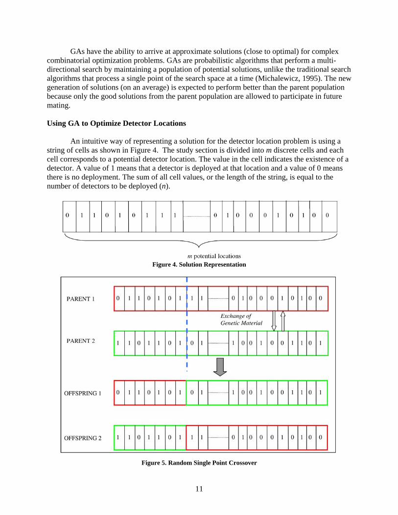
An intuitive way of representing a solution for the detector location problem is using a

string of cells as shown in Figure 4. The study section is divided into m discrete cells and each cell corresponds to a potential detector location. The value in the cell indicates the existence of a detector. A value of 1 means that a detector is deployed at that location and a value of 0 means there is no deployment. The sum of all cell values, or the length of the string, is equal to the number of detectors to be deployed (n).

Figure 4. Solution Representation

Figure 5. Random Single Point Crossover

12

The GA crossover procedure is illustrated in Figure 5. To introduce extra variability into the search population, a mutation operator is applied to the generated offspring with a probability (0.1-0.2) as shown in Figure 6.

Figure 6. Mutation

Case Studies

Case studies of freeway sections in two regions, Northern Virginia and Richmond, were conducted to demonstrate the developed method. In Northern Virginia, a section of I-66 from exit 43 to exit 57 in both directions; and in Richmond, a section of I-64 from exit 181 to exit 75, and a section of I-95 from exit 83 to exit 75 were studied.

Northern Virginia Case Study

An approximately 11-mile section of I-66 was studied in this project (Figures 7 and 8).

Three GPS equipped probe vehicles were driven on three week days during both the morning and evening peak periods in both the east and west directions. Vehicles departed at 5 minute headways. This resulted in a total of 37 travel time runs during the morning peak and 40 runs during the evening peak.

Since there are already detectors in place on this study section, existing detector locations

(spaced every half mile) were obtained and evaluated using the developed method. For the study section, the developed method was applied with the following objectives: (1) to determine the critical locations at which detectors need to be regularly maintained to obtain good travel time estimates, (2) to obtain the number and location of the optimal set of detectors for a given maintenance budget, and (3) to understand the impact of a critical detector malfunctioning on estimated travel times.

13

Figure 7. I-66 EB Study Section

Figure 8. I-66 WB Study Section

One of the main purposes of developing this methodology was to generate tradeoff plots between the travel time error and the number of detectors which would give the optimal placement of detectors for different levels of available funding. Tradeoff plots were generated by varying the actual number of detectors (q) from 2 to 20 in increments of 1. For each q, the GA was run for 200 generations with 200 individual solutions in each generation. On I-66, the peak period during the AM time period occurs in the eastbound (EB) direction (primarily commuter traffic going to Washington, DC) and the PM peak occurs in the westbound (WB) direction. Therefore, while determining the optimal detector locations on I-66 EB only the AM peak traffic patterns and prevailing speeds were considered. For I-66 WB the PM peak traffic patterns were used for the analysis. Results of the GA runs for the I-66 EB section are shown in Figures 9, 10, and 12. For a given number of detectors, the obtained optimal placement would result in a travel time estimation error for each travel time run. The maximum of these errors versus the detector deployment is plotted in Figure 9. As it can be seen from the plot, the maximum error value is high when only a few detectors are deployed; however, as the deployment increases the error value decreases. After reaching a certain level of deployment any further increase in the number of detectors may not decrease the error.

14

Figure 10 plots the frequency of travel time error over all travel time runs. It can be seen that as the deployment increases the plot becomes narrower with a mean value near zero. The decision makers can base their decisions on the deployment density based on these two figures. From Figures 9 and 10 it can be inferred that deploying 11 detectors would result in the least maximum TT error (~ 2 minutes) and an acceptable error distribution. The layout of the optimal set of detectors is shown in Figure 11. We can further conclude that the 20 detectors currently deployed are more than is needed to provide reasonably accurate travel time estimates. Figure 12 shows the number of times a potential detector location is present in the optimal solution. Of the 18 sets of detector deployments, for example, locations 18 and 20 are present in 16 and 17 sets, respectively. Location 18 corresponds to the detector located immediately downstream of the Rt. 7100 interchange (exit 55 on I-66) and location 20 is at the start of the Rt. 50 interchange (exit 57 on I-66). This is an indication that these locations are very critical for travel time computations and the detectors deployed in these locations need to be regularly maintained. To test the sensitivity of the optimal solution with respect to these critical detector locations, the optimization methodology was repeated with the condition that no detector can be placed at location 18. The error plots are shown in Figures 13 and 14. From Figure 13, it can be seen that the maximum error values are larger than the ones shown in Figure 9. The least maximum error, slightly higher than before, can be obtained by deploying 14 detectors, an increase of 3 detectors. Therefore, non-deployment or non-maintenance of detector at location 18 will result in inferior travel time estimates.

Figure 9. Maximum Travel Time Estimation Error Plot (I-66 EB AM Peak)

15

Figure 10. Estimated Travel Time Error Distribution Plot (I-66 EB AM Peak)

Figure 11. Location of the Optimal Set of Detectors for I-66 EB Study Section (11 Detectors)

In Figure 12 the x-axis corresponds to the detector location. The actual link number (from

Figure 7) corresponding to these detector locations can be obtained from Table 1.

16

Table 1. Link Numbers (Figure 7) Corresponding to Detector Numbers for I-66 EB Section

Figure 12. Frequency Plot showing the Number of Times a Detector is placed at Each Location (I-66 EB AM

Peak)

Figure 13. Maximum TT Error Plot for I-66 EB When No Detector is Placed at One Critical Location

(number 18)

17

Figure 14. Estimated TT Error Distribution Plot for I-66 EB When No Detector Is Placed at One Critical

Location (location 18)

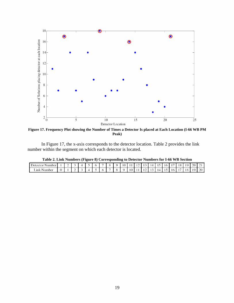
Results for the I-66 WB study section are shown in Figures 15, 16, and 17. From Figures 15 and 16 it can be inferred that deploying 14 detectors would result in the least maximum TT error of 35 seconds and an acceptable error distribution. This indicates that 7 detectors are redundant in the current deployment on this corridor. Figure 17 shows the number of times a potential detector location is present in the optimal solution. Of the 19 sets of detector deployments, locations 3, 9, 14, and 21 are present in 17, 18, 16, and 17 sets, respectively. The layout of the optimal placement of detectors for I-66 WB is shown in Figure 18.

18

Figure 15. Maximum Travel Time Estimation Error Plot (I-66 WB PM Peak)

Figure 16. Estimated Travel Time Error Distribution Plot (I-66 WB PM Peak)

19

Figure 17. Frequency Plot showing the Number of Times a Detector Is placed at Each Location (I-66 WB PM

Peak)

In Figure 17, the x-axis corresponds to the detector location. Table 2 provides the link number within the segment on which each detector is located.

Table 2. Link Numbers (Figure 8) Corresponding to Detector Numbers for I-66 WB Section

20

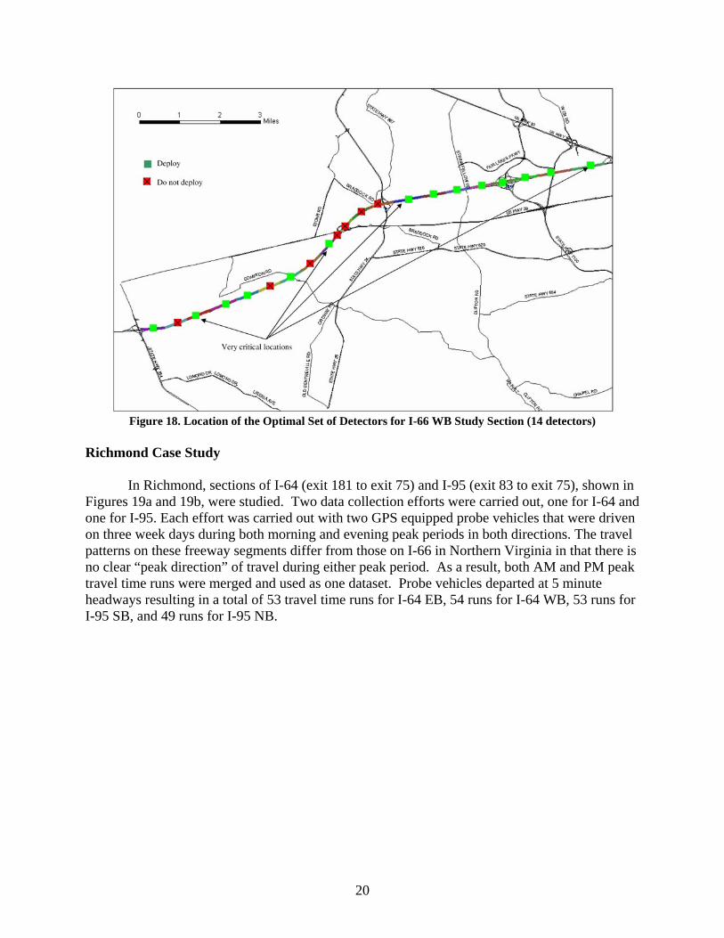
Figure 18. Location of the Optimal Set of Detectors for I-66 WB Study Section (14 detectors)

Richmond Case Study

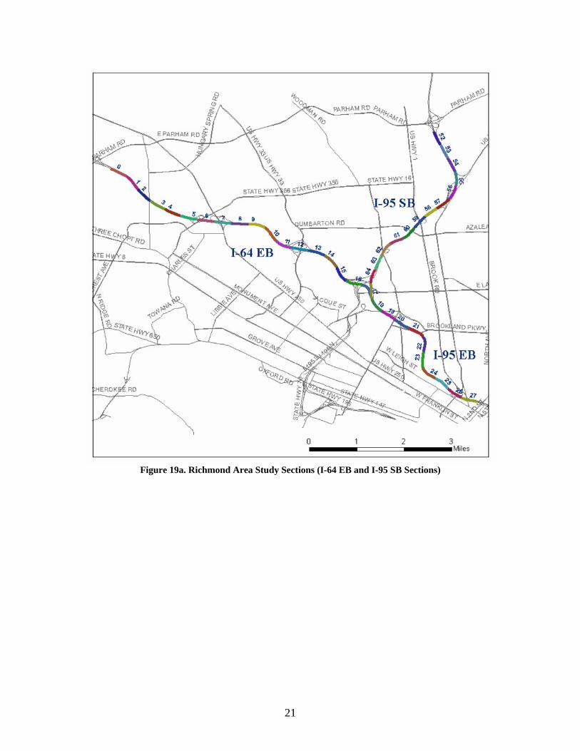
In Richmond, sections of I-64 (exit 181 to exit 75) and I-95 (exit 83 to exit 75), shown in Figures 19a and 19b, were studied. Two data collection efforts were carried out, one for I-64 and one for I-95. Each effort was carried out with two GPS equipped probe vehicles that were driven on three week days during both morning and evening peak periods in both directions. The travel patterns on these freeway segments differ from those on I-66 in Northern Virginia in that there is no clear “peak direction” of travel during either peak period. As a result, both AM and PM peak travel time runs were merged and used as one dataset. Probe vehicles departed at 5 minute headways resulting in a total of 53 travel time runs for I-64 EB, 54 runs for I-64 WB, 53 runs for I-95 SB, and 49 runs for I-95 NB.

21

Figure 19a. Richmond Area Study Sections (I-64 EB and I-95 SB Sections)

22

Figure 19b. Richmond Area Study Sections (I-64 WB and I-95 NB Sections)

Unlike the I-66 study section in Northern Virginia, study sections in Richmond currently

have very limited detector deployment. Therefore, the current locations of detectors were not considered as a constraint, and the research team used the methodology to find ideal locations from a “blank slate.” To do so, the team first divided the sections into segments of 0.3 mi each (recall from the methodology that this is the minimum sized segment that can be considered) with detectors placed at the mid-point of these segments. It is also important to note that the I-64 and I-95 study sections overlap (see Figures 19a and 19b). For the study sections, the developed methodology was applied to achieve the following objectives: (1) to determine the critical locations at which detectors need to be deployed and regularly maintained to obtain good travel time estimates, (2) to obtain the number and location of the optimal set of detectors for a given maintenance budget, and (3) to quantify how different the optimal placements for the overlap sections are and how to identify a compromise solution to achieve acceptable TT errors for both the I-64 and I-95 sections.

23

For the I-64 EB study corridor, the maximum travel time error plot (Figure 20) and the error distribution plot (Figure 21) show that placing 10 detectors would give an accurate estimate of travel times. The corresponding location of these 10 detectors as obtained from the optimization program is shown below in Table 3.

Table 3. Optimal Placement of Detectors on I-64 EB Study Section

Links 18 to 27 (see Figure 19a) are common to I-95 SB and I-64 EB. In this overlap

section detectors are placed on links 18, 20, 21, 24, and 27.

The number of times a potential detector location is present in the optimal solution is shown in Figure 22. Of the 26 sets of detector deployments, for example, location 18 is present in 25 of them. In Figure 22 the x-axis corresponds to the detector location. The actual link number (from Figure 19a) corresponding to these detector locations can be obtained from Table 4.

Table 4. Link Numbers (Figure 19a) Corresponding to Detector Numbers for I-64 EB

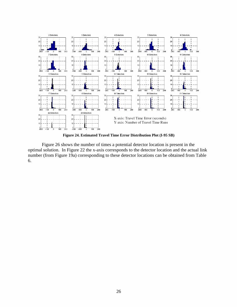
For the I-95 SB study corridor, the maximum travel time error plot and the error distribution plot are shown in Figure 23 and Figure 24, respectively. From these plots, two solutions are reviewed: 10 detectors and 15 detectors. While the results for deploying 15 detectors may be somewhat better than the results of deploying 10, the improvement may not be sufficient to justify the additional costs. The corresponding location of these detectors as obtained from the optimization program is shown in Table 5.

Table 5. Optimal Placement of Detectors on I-95 SB Study Section

In the common section (links 18 to 27) detectors are placed on links 18, 21, 22, 24, and 27 for the 10 detector solution and on links 18, 21, 22, 24, 25, 26, and 27 for the 15 detector solution.

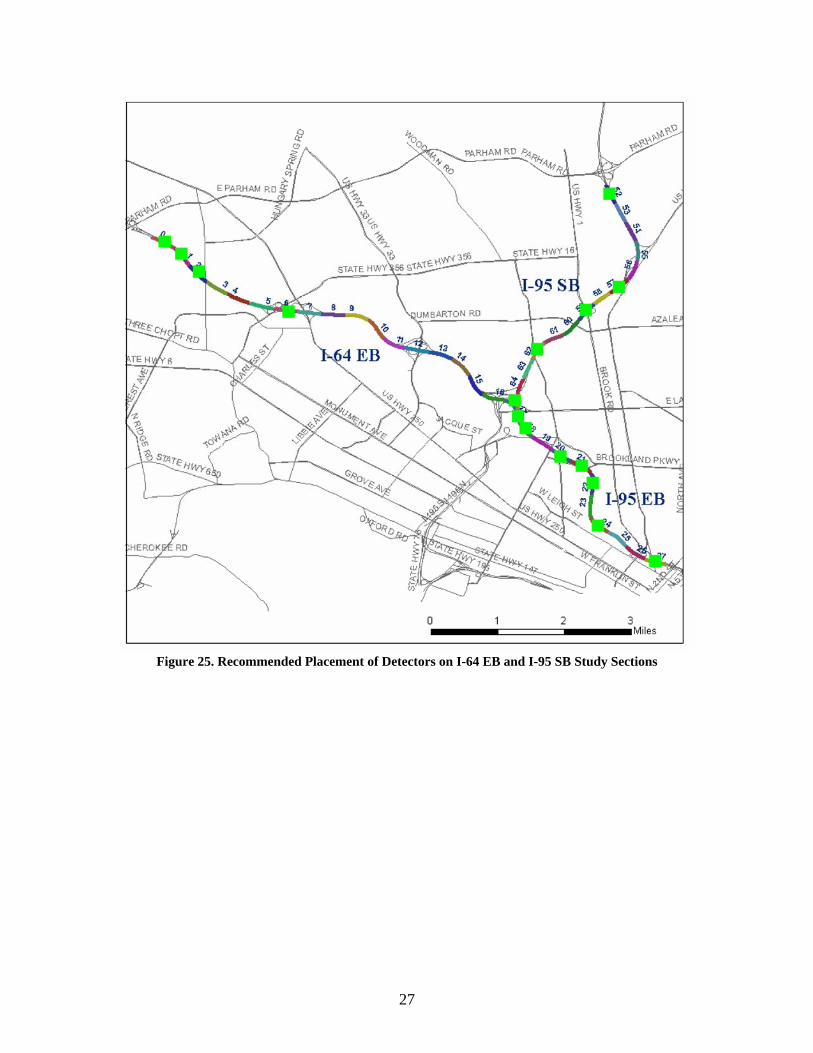
Comparing the optimal detector locations for I-64 EB and I-95 SB within the overlap section, it can be concluded that locations18, 21, 24, and 27 are crucial to obtain accurate TT estimates on both corridors. It is recommended that the detectors be placed at locations 18, 20, 21, 22, 24, and 27 so that optimal results are obtained for both corridors. The layout of optimal detector locations for these corridors is shown in Figure 25.

24

Figure 20. Maximum Travel Time Estimation Error Plot (I-64 EB)

Figure 21. Estimated Travel Time Error Distribution Plot (I-64 EB)

25

Figure 22. Frequency Plot Showing the Number of Times a Detector Is placed at Each Location (I-64 EB)

Table 6. Link Numbers (Figure 19a) Corresponding to Detector Numbers for I- 95 SB

Figure 23. Maximum Travel Time Estimation Error Plot (I-95 SB)

26

Figure 24. Estimated Travel Time Error Distribution Plot (I-95 SB)

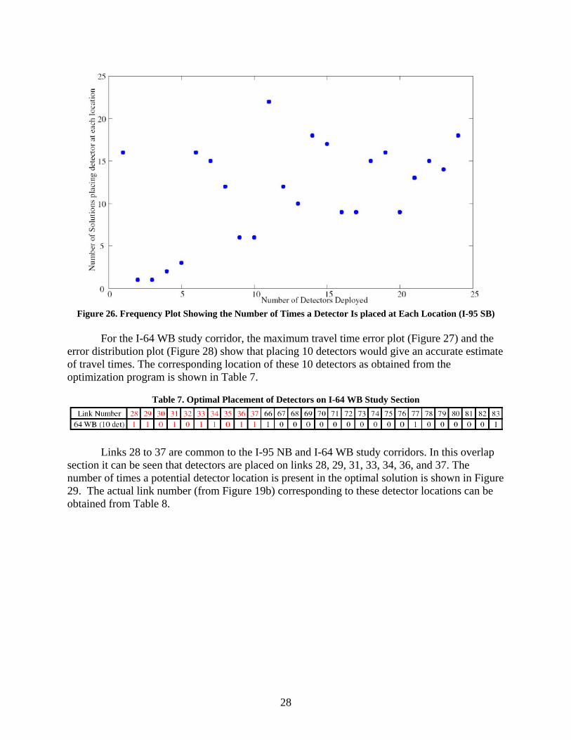
Figure 26 shows the number of times a potential detector location is present in the

optimal solution. In Figure 22 the x-axis corresponds to the detector location and the actual link number (from Figure 19a) corresponding to these detector locations can be obtained from Table 6.

27

Figure 25. Recommended Placement of Detectors on I-64 EB and I-95 SB Study Sections

28

Figure 26. Frequency Plot Showing the Number of Times a Detector Is placed at Each Location (I-95 SB)

For the I-64 WB study corridor, the maximum travel time error plot (Figure 27) and the

error distribution plot (Figure 28) show that placing 10 detectors would give an accurate estimate of travel times. The corresponding location of these 10 detectors as obtained from the optimization program is shown in Table 7.

Table 7. Optimal Placement of Detectors on I-64 WB Study Section

Links 28 to 37 are common to the I-95 NB and I-64 WB study corridors. In this overlap

section it can be seen that detectors are placed on links 28, 29, 31, 33, 34, 36, and 37. The number of times a potential detector location is present in the optimal solution is shown in Figure 29. The actual link number (from Figure 19b) corresponding to these detector locations can be obtained from Table 8.

29

Figure 27. Maximum Travel Time Estimation Error Plot (I-64 WB)

Figure 28. Estimated Travel Time Error Distribution Plot (I-64 WB)

30

Figure 29. Frequency Plot Showing the Number of Times a Detector Is placed at Each Location (I-64 WB)

Table 8. Link Numbers (Figure 19a) Corresponding to Detector Numbers for I-64 WB

For the I-95 NB study corridor, the maximum travel time error plot (Figure 30) and the error distribution plot (Figure 31) show that placing 13 detectors would give an accurate estimate of travel times. The corresponding location of these detectors as obtained from the optimization program is shown in Table 9.

Table 9. Optimal Placement of Detectors on I-95 SB Study Section

In the overlap section (links 28 to 37) detectors are placed on 28, 29, 30, 31, 32, 33, 34, 36, and 37. Comparing the optimal locations for the I-64 WB and I-95 NB corridors, it can be concluded that locations 28, 29, 31, 33, 34, 36, and 37 are crucial to obtain accurate TT estimates. It is recommended that the detectors be placed at locations 28, 29, 30, 31, 32, 33, 34, 36, and 37 so that optimal results are obtained for both corridors. The layout of optimal detector locations for these two corridors is shown in Figure 32.

31

Figure 30. Maximum Travel Time Estimation Error Plot (I-95 NB)

Figure 31. Estimated Travel Time Error Distribution Plot (I-95 NB)

32

Figure 32. Recommended Placement of Detectors on I-64 WB and I-95 NB Study Sections

The number of times a potential detector location is present in the optimal solution is

shown in Figure 33. The actual link number (from Figure 19b) corresponding to these detector locations can be obtained from Table 10.

Table 10. Link Numbers (Figure 19b) Corresponding to Detector Numbers for I-95 NB

33

Figure 33. Frequency Plot Showing the Number of Times a Detector Is placed at Each Location (I-95 NB)

CONCLUSIONS • The placement of detectors for the development of accurate travel time estimates will vary by

location based on specific traffic and geometric conditions. • With carefully placed detectors that are well maintained, travel time estimates can be derived

with an acceptable level of accuracy from point detection under non-incident conditions. Incident conditions were not specifically tested within the scope of this study. Given that traffic conditions change over time, detector placement will require periodic validation and possibly modification to ensure continued accuracy.

• The methods developed in this effort, including the GPS data collection and the mathematical

tool, were proven to be effective in determining preferred detector locations when the objective is to minimize travel time estimate error.

• In general, the developed method shows that the detector density needs to be higher in

congested areas of a corridor. Un-congested sections of the corridor need only a nominal deployment. Therefore, the general philosophy of more is better is only applicable for congested sections of freeway corridors. This was found to be true for both case studies – Northern Virginia and Richmond.

• It was found that detectors are required at merge areas near entrance ramps, especially when

the acceleration lanes are short. This can be attributed to the potential reduction in traffic speeds in merge areas due to increased weaving.

34

• For freeway corridors in Richmond, the minimum spacing of detectors was assumed to be 0.3 miles. As a result, the optimal detector locations recommended by the methodology can have some detectors separated by as little as 0.3 mile. The methodology can be applied for higher spacing (0.5 mile or 1 mile) depending on the available maintenance budget.

• One of the outputs of the method is the frequency plot that gives the number of times a

detector is placed at any location on the corridor for different sets of detectors. Locations with high frequencies are the ones that are most critical for deployment and/or maintenance.

• VDOT can reduce the number of detectors that are currently maintained by TMCs and can

deploy far fewer than the ½ mile spacing guidelines used in the past.

RECOMMENDATIONS 1. VDOT’s traffic management centers and regional operations planning staff should use the

tool developed in this study to determine future detector deployment strategies. Periodic re-evaluations of detector placement should be conducted to ensure that changes in traffic patterns and conditions have not resulted in degradation of the travel time estimates.

2. In locations such as Hampton Roads where extensive deployment of detectors exists, VDOT’s

regional operations staff should apply the tool to determine which detector locations are most critical in determining accurate travel time estimates. This set of detectors should then be considered as the “base” set of detectors, with other point detector locations added as other applications of the data demand.

3. VDOT’s northern region operations staff should concentrate maintenance efforts on those

detectors found to be critical in estimating travel time in this study and should expand the use of the tool to additional roadways in the region.

IMPLEMENTATION PLAN

Given the positive results of this research effort, the research team developed a plan to create a user-friendly computer application, and complementary user guidance/documentation, to assist VDOT personnel in identifying locations for detector placement. Personnel in the Smart Travel Laboratory will be guided by a VDOT steering committee comprised of technical personnel from the Northern Virginia, Hampton Roads, and Richmond Operations Regions to accomplish this. The following deliverables will be created to allow for implementation of the research:

• Web-based Computer Application. This computer application will operate on STL servers and be accessible via the Internet to VDOT field personnel. The application will allow personnel to input GPS tracks, identify locations of interest, and set key parameters to generate optimal detector locations.

35

• User’s Guide. A complete user’s guide will be developed to support personnel in utilizing the computer application. This guide will include specific examples for use in working with the application.

COSTS AND BENEFITS ASSESSMENT

VDOT has invested a significant amount of funds to the deployment of traffic flow detectors as part of the traffic management centers in Northern Virginia and Hampton Roads and is considering additional deployments in Richmond, Staunton, and Salem. While early justification for these devices was based on providing data for incident detection algorithms, more recently the focus has shifted to estimating travel time. The tool developed in this study indicates that substantially fewer detectors are needed for the travel time application than was true for incident detection. Using the results of the Northern Virginia case study on I-66 EB where there are 20 detector stations currently deployed, the tool identified minimum travel time errors when data are assumed to be coming from 11 of those stations, a reduction of 45%. Data from VDOT’s Traffic Monitoring System place the ongoing cost of a detector station at approximately $10,500. This results in an annual savings of $94,500 for this 11-mile roadway segment alone.

ACKNOWLEDGMENTS

This project could not have been accomplished without the assistance of numerous individuals. The authors thank Lance Dougald, Steve Griffin, and Arkopal Goswami for their assistance in data collection. The authors also express gratitude to Richard Steeg, Jim Smith, Dwayne Cook, Bob Sheehan, Ben Cottrell, Mike Perfater, and Linda Evans for their valuable comments on earlier drafts of this report that greatly helped in producing this final version.

REFERENCES Bartin, B, Ozbay, K., and Iyigun, C.A. Clustering Based Methodology for Determining the

Optimal Roadway Configuration of Detectors for Travel Time Estimation. In Proceedings of the 86th Annual Meeting of the Transportation Research Board, Washington, DC, 2007.

Chan, S., and Lam, H.K. Optimal Speed Detector Density for the Network with Travel Time

Information. Transportation Research A, Vol. 36, 2002, pp. 203-223. Ehlert, A., Bell, M., and Grosso, S. The Optimization of Traffic Count Locations in Road

Networks. Transportation Research B, Vol. 40, 2006, pp. 460-479.

36

Fujito, I., Margiotta, R., Huang, W., and Perez, W.A. The Effect of Sensor Spacing on Performance Measure Calculations. In Proceedings of the 85th Annual Meeting of the Transportation Research Board, Washington, DC, 2006.

Goldberg, D.E. Genetic Algorithms in Search, Optimization, and Machine Learning. Addison-

Wesley, Reading, MA, 1989. Li, R., Rose, G., and Sarvi, M. Evaluation of Speed-Based Travel Time Estimation Models.

Journal of Transportation Engineering, Vol. 132, No. 7, 2006. Liu, Y., Lai, X, and Chang, G.-L. Detector Placement Strategies for Freeway Travel Time

Estimation. In IEEE Intelligent Transportation Systems Conference, 2006. McGhee, C.C. Inventory of System Operations Data Collection and Use in the Virginia

Department of Transportation. VTRC 06-R21. Virginia Transportation Research Council, Charlottesville, 2006.

Oh, S., Ran, B., and Choi, K. Optimal Detector Location for Estimating Link Travel Speed in

Urban Arterial Roads. In Proceedings of the 82nd Annual Meeting of the Transportation Research Board, Washington DC, 2003.

ReVelle, C.S., and Eiselt, H.A. Location Analysis: A Synthesis and Survey. European Journal of

Operational Research, Vol. 165, 2005, pp. 1-19. Sherali, H.D., Desai, J., and Rakha, H.A. Discrete Optimization Approach for Locating

Automatic Vehicle Identification Readers for the Provision of Roadway Travel Times. Transportation Research Part B, Vol. 40, 2006, pp. 857-871.

Sisiopiku, V.P., Rouphail, N.M., and Santiago, A. Analysis of Correlation Between Arterial

Travel Time and Detector Data from Simulation and Field Studies. Transportation Research Record, No. 1457, 1994, pp. 166-173.

Thomas, G. The Relationship Between Detector Location and Travel Characteristics on Arterial

Streets. Institute of Transportation Engineering Journal, Vol. 169, 1999, pp. 36-42. Turner, S.M., Eisele, W.L., Benz, R.J., and Holdene, D.J. Travel Time Data Collection

Handbook. FHWA-PL-98-035. Federal Highway Administration, Washington, DC, 1998. Yang, H., and Zhou, J. Optimal Traffic Counting Locations for Origin-Destination Matrix

Estimation. Transportation Research Part B, Vol. 32, 1998, pp. 109-126.