Optimal Tariff with Heterogeneous Firms, Variable

Markups and Tariff-jumping FDI*

Ziran Ding†

University of Washington

November 7, 2018

Abstract

Variable markups and multinational production have gathered considerableattention in the trade literature, both because of their empirical prevalence andtheir welfare implication. In this paper, I study the optimal tariff in the pres-ence of variable markups and foreign direct investment. I then identify conditionsunder which protectionist trade policy, by changing the distribution of markups,and by inducing tariff-jumping FDI, may affect welfare. Three policy implicationsstand out from the analysis. First, if the initial protection level is sufficientlyhigh, an increase in home’s tariff will increase the number of tariff-jumping for-eign multinationals and decrease the number of foreign exporters, driving downthe average markup in the home market, and creating a pro-competitive effect.Second, whether zero tariff is socially optimal depends on consumer’s preference.Third, the promotion of FDI can reduce the non-cooperative tariff through a novelchannel: reducing the misallocation in the economy.

Keywords: Optimal tariff, Firm heterogeneity, Misallocation, Variable markup,Foreign direct investment

JEL Codes: F12, F13, F23, F60, R13

*I’m indebted to Theo Eicher, Fabio Ghironi and Mu-Jeung Yang for guidance, encouragementand continuous support. For helpful discussions, I thank Kristian Behrens, Keith Head, AntonioRodriguez-Lopez and seminar participants at UW International and Macro MTI Brownbag. All er-rors are my own.

†Address: Department of Economics, University of Washington, Savery Hall, Box 353330, Seattle,WA 98195-3330. Email: econjosh@uw.edu.

1

1 Introduction

What is the welfare implication of protectionist trade policy in an environment thatfeatures variable markups and foreign direct investment (FDI)? On the one hand,protectionism may hurt consumer welfare in the presence of variable markups if pro-tection results in higher market concentration. This has been a concern since AdamSmith, and it has received increasing attention in recent years1. On the other hand,in a highly-integrated global market2, foreign firms can avoid import tariffs by lo-cating production within the destination market. Such “tariff-jumping” activities3

can diminish the market power of domestic producers, thereby substantially mitigatewelfare consequences of the original trade protection policy.

The goal of this paper is to study the optimal tariff in the context of monopolisticcompetition, heterogeneous firms, variable markups, and FDI. To this end, the paperintroduces variable markups through quadratic quasi-linear preference, as in Melitzand Ottaviano (2008), into a two-country model with firm heterogeneity and FDI,as in Helpman et al. (2004). In the current framework, a firm needs to pay a fixedcost and draw its marginal production cost (which is inversely related to the firm’sproductivity) to enter the market. Post-entry, firms produce with different marginalcost levels. Exporters encounter two types of costs: iceberg-type trade cost and advalorem tariff. Multinationals face an iceberg-type of efficiency loss as in Keller andYeaple (2008). Firms formulate entry, export and FDI decisions based on expectedprofit. The difference in marginal cost preserves the sorting of firms4: the most pro-ductive firms access the foreign market through FDI, the less productive firms exportand the least productive firms only serve their domestic market. An increase in for-eign country’s tariff affects the variable profit of home exporters and multinationals,making FDI a more profitable entry mode for the most productive exporters, inducing

1Outside of the academic literature, increasing market concentration has received significant at-tention, e.g., A lapse in concentration (The Economist, September 2016), CEA (2016). In the academicliterature, see Asker et al. (2017), De Loecker and Eeckhout (2017) for recent evidence.

2Thanks to the growth of multinational firms. According to Antràs and Yeaple (2014), data from theU.S. Census Bureau indicates that roughly 90% of U.S. exports and imports flow through multinationalfirms, with close to one-half of U.S. imports transacted within the boundaries of multinational firmsrather than across unaffiliated parties.

3With the improvement in micro-level data availability, tariff-jumping FDI has received increasingempirical support, see Blonigen (2002), Belderbos et al. (2004), Hijzen et al. (2008) and more recently,Pietrovito et al. (2013), Alfaro and Chen (2015, 2018).

4In Helpman et al. (2004), the sorting of firms is preserved by the combination of fixed cost andvariable cost. Here, with bounded marginal utility, high-cost firms will not survive, even without suchfixed costs. The difference in marginal cost is sufficient to generate the sorting. Adding fixed cost willsubstantially degrade the tractability of the model, without generating additional insight.

2

tariff-jumping FDI under the heterogeneous firm framework.

The analysis of the findings shows that the welfare implication of protectionisttariff crucially depends on the assumption of entry. If entry and exit are restricted5,an increase in home import tariff makes it harder for the least productive foreignexporters to export. Those exporters will shut down their export department and onlyserve their domestic market. Meanwhile, an increase in home import tariff makesexport a less desirable entry mode for the most productive foreign exporters. Thosefirms will switch to FDI simply because the variable profit of FDI is higher thanthat of export. In the current setup, if the level of protection is low, the reduction offoreign exporters will dominate the increase of foreign multinationals, resulting in areduction of the total number of foreign firms in the home country. In equilibrium, theprotectionist trade policy creates an easier environment for domestic firms to survive.

The optimal level of protection depends on the markup distribution in the econ-omy. With a low protection level, an increase in home tariff reduces the total numberof foreign firms, creating a less competitive environment. As a result, the markupsof home’s domestic producers, foreign exporters and FDI firms all go up. In addition,exporters can pass the tariff burden on to consumers6. The average markup in theeconomy is affected by the composition effect. As the protection level increases, theshare of foreign exporters decreases, reducing the competition in the home market,and creating upward pressure on the average markup. At the same time, the shareof foreign tariff-jumping multinational firms increases, increasing the competition inthe home market, and creating downward pressure on the average markup. If thelevel of protection is high, the second effect can dominate the first, driving down theaverage markup in the economy. Protectionist trade policy can end up intensifyinghome market’s competition.

The current framework yields important implication for the pro-competitive ef-fect of trade. While recent studies on the welfare implication of trade liberalization7

emphasize the importance of variable markup, the insight here is that we shouldnot ignore the role of FDI. A decrease in home’s import tariff makes it easier for themost productive foreign domestic firms to export, increasing the number of foreign

5Restricted entry may also provide an adequate description of a short-run equilibrium in whichentry has not taken place yet and fixed costs are sunk, making exit never optimal. In this case, theeconomy is characterized by a fixed number and distribution of incumbents. These incumbents decidewhether they should operate and produce-or shut down. If so, they can restart production withoutincurring the entry cost again.

6 The degree of pass-through depends on firm’s specific productivity. Pass-through rate is lower formore productive firms. This is inline with the empirical evidence from De Loecker et al. (2016).

7For example, Edmond et al. (2015) and Arkolakis et al. (2018).

3

exporters serving home market, and creating a downward pressure to the home av-erage markup. At the same time, the reduction of tariff also makes it less desirablefor the least productive foreign multinationals to do FDI, decreasing the number offoreign FDI firms, and generating upward pressure to the home average markup. Ifthe initial protection level is sufficiently high, the decrease of multinational firmscan dominate the increase of exporters, driving up the average markup in the homemarket, and generating a negative pro-competitive effect.

When entry and exit are unrestricted, and the tariff revenue is redistributedto consumers, the number of entrants and the number of firms in the economy areendogenously determined by the tariff level. With the free-entry condition, an in-crease in home import tariff makes the home country a more desirable place to dobusiness, generating more domestic entry. Although the increase of home tariff stillmakes it harder for the least productive exporters to export, reduces the number offoreign exporters, and makes it easier for the most productive exporters to do FDI,and increases the number of foreign multinationals, the total impact on the numberof firms in the home market is dominated by the domestic entry. Different from therestricted entry case, the protectionist trade policy here creates more entry, gener-ates more competition in the home market, and makes it harder for local producersto survive.

With free-entry, trade policy implication depends on the efficiency of the econ-omy. The market is not efficient due to several distortions: (1) inter-sectoral dis-tortion: the markup-pricing in the differentiated-good sector distorts the allocationbetween the differentiated-good sector and homogeneous-good sector, implying aninefficiently small size of the monopolistically competitive sector; (2) intra-sectoraldistortion: due to variable markups, if consumers have a strong preference towardthe differentiated varieties, the market outcome can be inefficient in several dimen-sions compared to the socially optimal allocation: (i) weak selection in domestic, ex-port cutoff, and over-selective in FDI cutoff, (ii) oversupplies high-cost varieties andundersupplies low-cost varieties, (iii) oversupplies the total number of varieties andfeatures excessive entry

These market failures stem from several externalities: (i) on the supply side,both the markup-pricing and business-stealing effect tend to create too many vari-eties in the economy, (ii) on the demand side, the “love of variety” from the quadraticquasi-linear preference tends to create insufficient varieties in the economy, (iii) withvariable markup, the market outcome oversupplies varieties produced by less pro-ductive firms, resulting in inefficiently large size for these firms. These externalities

4

collectively result in the inefficiencies in the market outcome. In contrast, under CESpreference, the market outcome produces the same allocation as the social planner.

Two general policy implications stand out from the analysis. First, free tradeis not always socially optimal. Although a decrease in tariff can generate entry inthe economy, and improve consumer welfare, it also takes away the profits of exist-ing firms. If the relative demand for the differentiated varieties is sufficiently high,the negative effect on firms can outweigh the positive impact on consumers, therebydecreasing the social welfare. In this case, protectionist trade policy can be welfare-improving by deterring the excessive entry.

Second, the promotion of FDI can lower a country’s non-cooperative tariff levelwhen economy features misallocation. If the relative demand for the differentiatedvarieties is sufficiently high, the market economy oversupplies high-cost varieties. Inthis case, misallocation materializes as less productive firms are allocated with toomany resources (labor). If the Pareto distribution parameter k is small (higher de-gree of firm heterogeneity), then there are relatively more productive firms in theeconomy. Since tariff-jumping FDI happens among the more productive firms alongthe marginal cost distribution, the tariff-jumping foreign firms now utilize more homelabor. In this case, home labor is reallocated toward more productive firms, reducingthe misallocation in the home economy. The reduction of misallocation has a moresignificant impact on the economy compared to the case when k is large (lower de-gree of firm heterogeneity). The Nash tariff under smaller k is lower than the Nashtariff under bigger k. This shows when the economy features a higher degree of firmheterogeneity (smaller k), hence a higher degree of misallocation, allowing firms toengage in FDI can lower the non-cooperative tariff level.

The rest of the paper proceeds as follows. Section 2 contrasts the current ap-proach to the related literature. Section 3 describes the benchmark model and char-acterizes the equilibrium. Section 4 studies the equilibrium features of the model.Section 5 studies the composition effect under a tariff change, socially optimal tariff,and Nash tariff with and without FDI under symmetry. Section 6 further exploresthe role of variable markups in the current setup. Section 7 concludes.

2 Related Literature

The findings in this paper are related to, and have implications for, a large num-ber of papers in the trade policy literature. Many authors have studied the trade

5

policy implication with heterogeneous firms framework, for example: Demidova andRodriguez-Clare (2009) use a Melitz-type model and a small country assumption toshow the first-best outcome can be achieved through either a consumption subsidy, ex-port tax, or an import tariff; Felbermayr et al. (2013) allow for Melitz-type large coun-tries and characterize a link between the level of Nash import tariffs and parametersrelated to transportation costs and productivity dispersion; Bagwell and Lee (2015)study trade policy in Melitz and Ottaviano (2008) model and provides a rationale forthe treatment of export subsidies within the World Trade Organization;Costinot et al.(2016) utilize a generalized Melitz model to characterize optimal unilateral tariffsboth when tariffs are firm-specific and when they are industry-specific. They identifya central role for the terms-of-trade externality in their analysis of unilateral trade-policy intervention. Demidova (2017) studies the optimal tariff in the Melitz andOttaviano (2008) environment without the outside good and finds protection is al-ways desirable, and reductions in cost-shifting trade barriers are welfare-improving.A common feature of the aforementioned papers is their exclusive focus on domesticproducers and exporters. A key message from the current analysis is that ignoring themultinational production may provide a misleading picture of the protectionist tradepolicy. The findings in this paper show that the promotion of FDI can effectively lowerthe non-cooperative tariff level.

A recent article by Cole and Davies (2011) is closely related to the current paper.The authors introduce ad valorem tariff and heterogeneous fixed costs into Helpmanet al. (2004), and find equilibria in which both pure exporters and multinationalscoexist, resolving a known puzzle8 in the strategic tariff literature in the presenceof multinationals. Heterogeneous fixed costs for exporters and multinationals is thekey element to generate their result. In contrast, the coexistence of exporters andmultinationals in the current framework comes from the different iceberg costs theyare facing.

Despite the apparent similarity between the two frameworks, it should be clearthat the two exercises are very different. First, Cole and Davies (2011) utilize quasi-linear CES preference, combining with monopolistic competition, yielding constantmarkups and complete pass-through in equilibrium. Despite its analytical tractabil-ity, the combination of CES and monopolistic competition has little merit, even as afirst approximation, for welfare analysis. In contrast, the current framework utilizesquadratic quasi-linear preference to generate heterogeneous firms and incompletepass-through for different firms, which is more suitable for pricing and welfare anal-

8In equilibrium, all foreign firms are either multinationals or exporters.

6

ysis. Second, Cole and Davies (2011) completely ignore the potential for tariffs toimpact entry. According to Caliendo et al. (2017), the combination of ad valorem tar-iff and tariff rebate violates the macro assumption in ACR, the level of entry shouldnot remain fixed in Cole and Davies (2011). In the current framework, the number ofentrants is endogenously affected by tariff level, generating different welfare implica-tion for protectionist trade policy in the short run and long run. Third, the presence ofvariable markup alters the free trade implication. Cole and Davies (2011) find sociallyoptimal tariff is always to subsidize trade. This is because trade can foster competi-tion and eliminate the least productive firms, increasing aggregate productivity. Inthe current framework, whether free trade is socially optimal depends on consumer’srelative demand for the differentiated varieties. Subsidizing trade is desirable onlywhen there is an insufficient entry in the economy.

The role of variable markup has received increasing attention in the interna-tional trade literature. For example, Arkolakis et al. (2018) show that the undera large class of demand function, the non-homothetic preference dampens the pro-competitive effect of trade liberalization (incurred by the change of iceberg-type tradecost) by increasing the degree of misallocation. Edmond et al. (2015) show that thesize of the pro-competitive gain9 can be quite large in the presence of significant mis-allocations and weak cross-country comparative advantage in individual sectors. Dif-ferent from these two papers, the current framework shows that the pro-competitiveeffect of trade can be very different when FDI is incorporated.

Lastly, the welfare implication of FDI is an old topic in the field, see e.g., Brecherand Alejandro (1977). Some recent papers have revisited the welfare impact of FDI,either analytically or quantitatively. Ramondo and Rodríguez-Clare (2013) show thatwhen taking account of the multinational production, the gains from openness arearound twice the gains calculated in trade-only models. Irarrazabal et al. (2013) ex-tend Helpman et al. (2004) to allow intra-firm trade and structurally estimate theirmodel using firm-level data from Norwegian manufacturing sector. Their counterfac-tual analysis indicates that impeding FDI has substantial effects on trade flows butnot on welfare. Different from their exercises, this paper studies explicitly the welfareimplication of FDI through the interaction with the tariff. The paper identifies a newsource of welfare gain of FDI: through resource allocation by reducing the degree ofmisallocation in the economy.

9According to their setup, a pro-competitive gain is associated with a lower average markup.

7

3 The Model

This section introduces quadratic quasi-linear preference into Helpman et al. (2004)framework. There are two symmetric countries, home (H) and foreign (F ). The mar-kets are segmented, and international trade entails trade costs that take the form oftransportation costs as well as ad valorem import tariffs. Tariff revenue is distributedequally across consumers in the tariff-imposing country. FDI incurs an iceberg-typeof marginal cost (i.e., efficiency loss) in the spirit of Keller and Yeaple (2008). Dif-ferent from Cole and Davies (2011), where firms’ partition is induced by differentfixed cost, the non-homothetic preference here induces different productivity cutoffsthrough different marginal cost.

3.1 Consumers

Consider the H economy with one unit of consumers, each supplies 1 unit of labor.Consumers in country H choose over qH0 and qHi

UH = qH0 + α

∫i∈ΩH

qHi di−1

2γ

∫i∈ΩH

(qHi)2di− 1

2η

(∫i∈ΩH

qHi di

)2

subject to: qH0 +

∫i∈ΩH

pHi qHi di ≤ IH ≡ wH + TRH + ΠH

where α and η indicate the substitutability between the differentiated varieties andnuméraire good, γ indicates the substitutability among the differentiated varieties.An increase in α and a decrease in η both shift out the demand for the differentiatedvarieties relative to the numéraire. Notice that different from Melitz and Ottaviano(2008), the tariff revenue and aggregate profit will enter into consumer’s budget con-straint through government transfer.

Assuming consumers have positive demands for the numéraire good(qH0 > 0

),

maximization of the above problem leads to the following inverse demand for eachvariety i:

pHi = α− γqHi − ηQH (1)

where QH ≡∫i∈ΩH q

Hi di is the aggregate consumption of these varieties. Invert equa-

8

tion (1) to obtain the linear market demand for these varieties

qi ≡ qHi =α

ηNH + γ− 1

γpHi +

ηNH

ηNH + γ

1

γpH

=1

γ

(pHmax − pHi

)(2)

where pHmax = (γα + ηNH pH)/(ηNH + γ) represents the price at which demand for avariety is driven to 0, pH ≡ (1/NH)

∫i∈ΩH p

Hi di is the average price of all consumed

variety in country H, and ΩH is the consumed subset of ΩH . Note that equation (1)also implies pHmax ≤ α. Different from CES preference, where the elasticity of demandis constant, the price elasticity of demand here is given by

εHi ≡∣∣∣∣∂qHi∂pHi

× pHiqHi

∣∣∣∣ =1

pHmax/pHi − 1

(3)

The lower the average price pH or a larger number of competing varieties NH inducea decrease in the price bound pHmax and an increase in the price elasticity of demandεHi at any given pHi . These all represent a “tougher” competitive environment, whichcan’t be captured in an environment with constant elasticity of demand.

As in Melitz and Ottaviano (2008), welfare can be evaluated using the followingindirect utility function:

UH = IH +1

2

(NH

ηNH + γ

)(α− pH

)2+

1

2

NH

γσ2pH (4)

where σ2pH ≡

(1/NH

) ∫i∈ΩH

(pHi − pH

)2di represents the variance of prices. To ensure

positive demand levels for the numéraire, I assume that IH >∫i∈ΩH p

Hi q

Hi di = pHQH −

NHσ2pH/γ. The welfare will be higher when the average price pH is lower, the variance

of prices σ2pH is higher and the number of variety NH is larger.

3.2 Firms

Production in the economy only utilizes labor, which is supplied in an inelastic fash-ion in a competitive market. qH0 is produced under a constant return to scale tech-nology at unit cost. Thus the wage10 in each country equals to one: wH = 1. In the

10If I drop the numéraire good, wage will be endogenized and can be pinned down by trade balancecondition.

9

differentiated-good sector, firms operate under monopolistic competition, and eachfirm produces a single variety. To enter the market, a firm needs to pay a fixed costfE > 0 and draws its marginal production cost c, which indicates the unit labor re-quirement. The cost is drawn from a Pareto distribution with cumulative distributionfunction G(c) = (c/cM)k, where k ≥ 1 represents a shape parameter and cM > 0 rep-resents the upper bound of c. When k = 1, the marginal cost distribution is uniformon [0, cM ]. As k increases, the relative number of low productivity firms increases, andthe distribution is more concentrated at these lower productivity levels. I assume Hand F share the same technology, hence the same upper bound cM and the same fE.

Depending on its productivity draw, a firm enters country H may exit, producelocally, export to country F or engage in the multinational activity. Following Melitzand Ottaviano (2008), I assume markets are segmented, and firms operate undermonopolistic competition in each market. Therefore, a firm makes separate decisionsabout its prices at each market, taking the total number of varieties and the averageprice in a market as given.

3.2.1 Domestic Producer

A firm located in country H with cost level c selects its price in the domestic market,pHD , to maximize its domestic profit πHD (c) =

[pHD(c)− c

]qHD (c). Together with equation

(2), the optimal price, markup, quantity, hence profit are:

pHD (c) =1

2

(cHD + c

)(5)

mHD (c) =

1

2c

(cHD + c

)(6)

qHD (c) =1

2γ

(cHD − c

)(7)

πHD (c) =1

4γ

(cHD − c

)2 (8)

Let cHD ≡ supc : πHD (c) > 0

represent the cost of the firm who is indifferent about

remaining in the market. This firm earns zero profit as its price is driven downto marginal cost, together with equation (2), pHD

(cHD)

= cHD = pHmax. Hence, a firmwill only serve domestic market if c ≤ cHD . As expected, lower cost firms set lowerprices and earn higher profits. However, lower cost firms do not pass all of the costdifferentials to the consumer, and they also charge higher markups (which is defined

10

as m(c) = p(c)/MC(c), decreasing in c).

3.2.2 Exporter

The exporter in country H will face an ad valorem import tariff imposed by countryF , denoted as tF ≥ 1. On top of that11, the exporter will also face a per-unit tradecost12, denoted by τF . More specifically, the delivered cost of a unit cost c to countryF is τF c where τF > 1. A firm maximizes its profit πHX (c) =

[pHX(c)/tF − τF c

]qlX(c) by

choosing optimal price pHX(c). Together with equation (2), the optimal price, markup,quantity, hence profit are:

pHX (c) =tF τF

2

(cHX + c

)(9)

mHX (c) =

tF

2c

(cHX + c

)(10)

qHX (c) =tF τF

2γ

(cHX − c

)(11)

πHX (c) =tF(τF)2

4γ

(cHX − c

)2 (12)

Let cHX ≡ supc : πHX (c) > 0

denotes the upper bound cost for exporters from H to F.

Combine it with the definition of cFD (parallel to cHD), this cutoff then satisfies cHX =

cFD/tF τF : tariffs and transportation cost make it harder for exporters to break even

relative to the domestic market.

3.2.3 Multinational

To engage in the multinational activity, a firm located in country H with cost level cchooses its product price for consumers in country F, denoted as pHFDI(c). Instead ofserving foreign market through exports, it directly serves locally in country F, butdoing so will incur a higher marginal cost13, ϕF . Here, I assume ϕF > τF to ensure

11To ensure that when the net tariff is zero, there’re still exporters in the economy, I need to introducethe iceberg-type of transportation cost.

12Following Melitz and Ottaviano (2008), I abstract from any fixed export cost, which would sub-stantially reduce the tractability of the model without adding additional insights. With the boundedmarginal utility, different marginal costs are enough to induce the sorting of firms.

13This feature is similar to Keller and Yeaple (2008), who shows that when technologies are complex,it is more difficult for US-owned foreign affiliates to substitute local production with imports from

11

there’re still multinational firms in the economy even when the net tariff is zero.Multinational firm’s profit function is as follow:

πHFDI (c) =[pHFDI (c)− ϕF c

]qHFDI (c) (13)

Together with equation (2), the optimal price, markup, quantity, hence profit are:

pHFDI (c) =1

2

(cFD + ϕF c

)(14)

mHFDI (c) =

1

2ϕF c

(cFD + ϕF c

)(15)

qHFDI (c) =1

2γ

(cFD − ϕF c

)(16)

πHFDI (c) =1

4γ

(cFD − ϕF c

)2 (17)

Let cHFDI = supc : πHFDI(c) > πHX (c)

denote the upper bound cost for multinational

from H to F. Combine with the definition of cFD, this cutoff then satisfies cHFDI = ξF cFD,

where ξF ≡ (1−√tF )/(tF τF −

√tFϕF ) is derived by setting πHFDI(c) = πHX (c).

Note, there are two possible cases in this solution, cHFDI = (1 ±√tF )/(tF τF ±√

tFϕF )cFD, but only one of them is interesting and relevant here. According to theprediction in Helpman et al. (2004), for those firms that serve foreign markets, onlythe most productive ones engage in FDI14. In the current setup, this implies cHFDI <cHX < cHD . Compare the expression of cHX and cHFDI , both cases imply ϕF > tF τF , whichincorporates the previous assumption that ϕF > τF since tF ≥ 1. However, for the caseof cHFDI = (1 +

√tF )/(tF τF +

√tFϕF )cFD, cHFDI will decrease in response to an increase in

tF , indicating the marginal multinationals will choose to become exporters when tariffincreases. This is at odds with the empirical evidence15 of tariff-jumping. Therefore,the other choice cHFDI = (1−

√tF )/(tF τF −

√tFϕF )cFD makes more sense here since cHFDI

will increase in response to an increase in tF , in line with the empirical evidence of

multinational headquarter. ϕF can also stand for the information costs of working broad, transactioncosts of dealing with FDI policy barriers, costs of maintaining the affiliate, servicing network costs,and other costs associated with technology costs in offshore production.

14This pattern also receives empirical support, see Doms and Jensen (1998) for the U.S. and Conyonet al. (2002) for the U.K, for more recent evidence, see Mataloni (2011).

15For example, Blonigen and Feenstra (1997), Barrell and Pain (1999) consistently find substantialtariff-jumping responses. Blonigen (2002) finds smaller average tariff-jumping responses and con-cludes that tariff-jumping is a realistic option for multinational firms from industrialized countries.Blonigen et al. (2004) find tariff-jumping in the form of new plants or plant expansion has significantlylarger negative effects on U.S. domestic firms’ profits.

12

productivity sorting and the tariff-jumping FDI. The following graph indicates theregion that FDI will occur and the relation between t, ϕ, and τ for FDI to happen:

Figure 1: Minimum Tariff to Induce Tariff-jumping FDI

Discussion on firm’s FDI motivation here is important. In Helpman et al. (2004),the sorting of firms is preserved under the assumption of fI > τ ε−1fX > fD. Exportincurs a higher marginal cost (τ ), but as long as the fixed cost of FDI, fI , is suffi-ciently high, they can still guarantee the most productive firms find FDI more de-sirable than export. This is a classic proximity-concentration tradeoff in the spiritof Brainard (1997). The similar tradeoff is also present in Cole and Davies (2011),where the authors embed ad valorem and variable fixed cost into the Helpman et al.(2004) framework. They find as the tariff increases, the variable profit of exporterdecreases while the differences in fixed cost remain the same. When the tariff level issufficiently high, the gain from avoiding the tariff is higher than the fixed cost of be-coming a multinational, and a firm prefers FDI over export as an entry mode. In thecurrent setup, this is no longer the case. Comparing the profit function for exporterand multinational:

πHX (c) =[pHX(c)/tF − τF c

]qHX (c) (18)

πHFDI (c) =[pHFDI (c)− ϕF c

]qHFDI (c) (19)

As tariff increases, the revenue of exporter will drop, making export a less desirablemode of accessing foreign market. Eventually, FDI becomes a more desirable entry

13

mode. Although the marginal cost of FDI is higher than export (ϕF > τF ), the oper-ating profit of FDI exceeds the profit of export. The tradeoff between export and FDIis merely a comparison between the profits, no longer the conventional proximity-concentration tradeoff.

The underlying reason that FDI is a valid option for the firm is discussed in Mrá-zová and Neary (2018). They argue that “...statements like “Only the more productivefirms select into the higher fixed-cost activity” are often true, but always misleading:they are true given Super-modularity16, but otherwise may not hold. What mattersfor the direction of second-order selection effects 17 is not a trade-off between fixed andvariable costs, but whether there is a complementarity between variable costs of pro-duction and of trade. Putting this differently, for FDI to be the preferred mode ofmarket access, a firm must be able to afford the additional fixed costs of FDI 18, butwhether it can afford them or not depends on the cross-effect on profits of tariffs andproduction costs. When Super-modularity prevails, a more efficient firm has relativelyhigher operating profits in the FDI case, but when sub-modularity holds, the oppositemay hold. ” The reason that the current setup can preserve the conventional sorting(i.e., second-order selection effect) is primarily due to the Super-modularity of profitfunction (as in Mrázová and Neary (2018), Section 6) since there exists complemen-tarity between variable costs of production and of trade.

3.3 Free Entry Condition

Entry is unrestricted in both countries. Firms choose a production location be-fore entry and paying the sunk entry cost. To restrict the analysis on the effects oftrade costs differences, I assume that countries share the same technology19 (i.e., thesame entry cost fE and the same cost distribution G(c)). Free entry of domestic firms

16For the definition of Super-modularity and later on, sub-modularity, please refer to Mrázová andNeary (2018).

17According to their description, this is referring to the choice of export vs. FDI.18Their setup is a general preference, so they rely on fixed cost. In Appendix F, they mentioned Melitz

and Ottaviano (2008) and pointed out the first-order selection effect (according to their description, thisis referring to whether serve the foreign market or not) with quadratic quasi-linear preference needsthe existence choke price.

19For implications of Ricardian comparative advantage, please refer to the Appendix in Melitz andOttaviano (2008).

14

in country H implies zero expected profits in equilibrium, hence:∫ cHD

0

πHD (c) dG (c) +

∫ cHX

cHFDI

πHX (c) dG (c) +

∫ cHFDI

0

πHFDI (c) dG (c) = fE (20)

Given the Pareto assumption in both countries, the free entry condition for country Hcan be rewritten as:

(cHD)k+2

+ ΦF1

(cFD)k+2

+ ΦF2

(cFD)k+2

= γφ (21)

where φ ≡ 2 (k + 1) (k + 2) (cM)k fE is a technology index that combines the effects ofthe better distribution of cost draws (lower cM ) and lower entry costs fE. Moreover,

ΦF1 ≡

(k + 1) (k + 2) tF (τF )2

2

(1

tF τF

)k+2

−(

1

tF τF

)2 (ξF)k

− 2k

k + 1

[(1

tF τF

)k+2

−(

1

tF τF

)(ξF)k+1

]+

k

k + 2

[(1

tF τF

)k+2

−(ξF)k+2

]

ΦF2 ≡

(k + 1) (k + 2)(ξF)k

2

[1− 2kϕF ξF

k + 1+k(ϕF ξF

)2

k + 2

]

are indices that combine the trade-off between tariff and higher marginal cost of FDI.The free entry condition is homogenous to degree k + 2 regarding the cutoffs. Thissystem (for H,F ) can then be solved for the cutoffs in both countries:

cHD =

[γφ

1−(ΦF

1 + ΦF2

)1− (ΦF

1 + ΦF2 ) (ΦH

1 + ΦH2 )

] 1k+2

(22)

Two observation stand out in comparison to Melitz and Ottaviano (2008): (1) Thiscutoff is lower20 than the closed-economy cutoff21, indicating the opening up of aneconomy via export and multinational activity will increase the aggregate productiv-ity by forcing the least productive firms to exit. This result is similar to Melitz (2003)but works through product market competition, instead of factor market competi-tion, as argued in Melitz and Ottaviano (2008). (2) This cutoff is even lower22 than

20This is based on Lemma 1, see Appendix A.1.21See equation (15) in Melitz and Ottaviano (2008), which is cHD = (γφ)

1/(k+2). The difference is thatI normalized the labor size to be one.

22See Appendix A.1 for the proof.

15

the open economy cutoff23 generated in Melitz and Ottaviano (2008). The intuitionis straightforward: the presence of FDI, here the most productive firms in the dis-tribution, intensifies the competitive environment in the economy, forcing the leastproductive firms to exit and hence further increases aggregate productivity.

3.4 Prices, Product Variety, Number of Entrants and Welfare

To see more features in the current setup, I first compute pH . Notice, the costof H ’s firms c ∈ [0, cHD ] , the delivered cost of exporters τF c ∈ [0, cHD ] and the cost ofmultinationals ϕF c ∈ [0, cHD ] all share identical distributions over the support givenby GH(c) = (c/cHD)k. The price distribution of H ’s domestic firms, pHD(c) , and exportersproducing in F , pFX(c) and F ’s multinationals producing in H, pFFDI(c), are thereforeall identical. The average price in country H is thus given by:

pH =1

G (cHD)

∫ cHD

0

pHD (c) dG (c) =1

G (cFX)

∫ cFx

cFFDI

pFX (c) dG (c)

=1

G (cFFDI)

∫ cFFDI

0

pFFDI (c) dG (c) =2k + 1

2k + 2cHD (23)

Combining this with the definition of pHmax and pFmax, the number of firms selling incountry H is:

NH =2γ(α− cHD

)(k + 1)

ηcHD(24)

From this expression, it must be the case that α > cHD so that the number of firmsselling in country H is positive in equilibrium. The number of product variety incountry H is composed of domestic producers, exporters, and multinationals fromcountry F . Given a positive mass of entrants NE in both countries, there are G(cHD)NH

E

domestic producers, [G(cFX) − G(cFFDI)]NFE exporters, and G(cFFDI)N

FE multinationals

selling in H satisfying:

G(cHD)NHE +

[G(cFX)−G

(cFFDI

)]NFE +G

(cFFDI

)NFE = NH (25)

23See equation (23) in Melitz and Ottaviano (2008), which is cHD =[γφ(1− ρF

)/(1− ρHρF

)]1/(k+2)

when labor is normalized to one. The open economy cutoff is slightly different due to the ad valoremtariff, see Appendix A.1 for details.

16

Solving this system (for H and F ) will give us the number of entrants in country H:

NHE =

2 (cM)k (k + 1) γ

η (1− δHδF )

[α− cHD(cHD)

k+1− δH α− c

FD

(cFD)k+1

](26)

where δl = (tlτ l)−k, for l ∈ H,FNotice, to ensure positive mass of entry in theequilibrium, it is straightforward to show that α > clD for l = H,F . This implicationis crucial in understanding the equilibrium feature of the model. I will come backto this point in Section 3. Following Melitz and Ottaviano (2008), combine (4), (23),(24) and the definition of σ2

pH , it is straightforward to show the consumer welfare in H

equals to:

UH = IH +α− cHD

2η

(α− k + 1

k + 2cHD

)︸ ︷︷ ︸

≡CSH

(27)

Once again, welfare changes monotonically with the domestic cutoff, which capturesthe effect of an increase in product variety and a decrease in the average price. Alsonotice, consumer surplus in country H is given by the second term in equation (27).

3.5 Tariff Revenue and National Welfare

This part will be particularly important when analyzing socially optimal tariffand Nash tariff. Note that tariff revenue is also a component of consumer income IH

through the redistribution from the government. I define the pre-tax value of countryH ’s import as:

IMH = NFE

∫ cFX

cFFDI

pFX (c)

tFqFX (c) dG (c)

= NFE

tH(τH)2 (

cHD)k+2

4γ (k + 2) (cM)k

[2

(1

tHτH

)k+2

− k + 2

(tHτH)2

(ξH)k

+ k(ξH)k+2

](28)

Therefore, the total important tariff revenue of country H is defined as

TRH ≡ (tH − 1)× IMH

= NFE

tH − 1

tH

(cHD)k+2

4γ (k + 2) (cM)k

[2

(1

tHτH

)k− (k + 2)

(ξH)k

+ k(ξH)k+2 (

tHτH)2

](29)

17

From the trade-policy perspective, the government will consider the following con-sumer welfare function as its criterion:

UHn = wH + (tH − 1)× IMH + ΠH︸ ︷︷ ︸

≡IH

+α− cHD

2η

(α− k + 1

k + 2cHD

)︸ ︷︷ ︸

≡CSH

(30)

Therefore tariff affects consumer welfare from two channels: (1) consumer surplus,which is directly affected by the change in cHD in response to tariff; (2) tariff revenue,which is affected by both the tariff level (tH) and the tariff base (IMH). Due to free-entry condition, aggregate profit ΠH is driven to zero in equilibrium. Notice due to thepresence of numéraire good, wH = 1. Consumers will not take tH into considerationwhen maximizing their utility. However, the government does choose the optimaltariff level to achieve highest national welfare objective function.

With the model above, I will now discuss the equilibrium features of this econ-omy, contrast it with an economy features heterogeneous firms, FDI but constantmarkups, as in Cole and Davies (2011). Then I will discuss the welfare implicationfor trade policy in the current setup.

4 Equilibrium Conditions

The presence of FDI tends to intensify the degree of competition in the economy.

Lemma 1. The presence of FDI makes the economy more competitive, the domesticcutoff is lower compared to the case when there is no FDI:

cHD1 =

[γφ

1−(ΦF

1 + ΦF2

)1− (ΦF

1 + ΦF2 ) (ΦH

1 + ΦH2 )

] 1k+2

< cHD2 =

[γφ

1− ψF

1− ψFψH

] 1k+2

Proof. See Appendix A.1

In the Appendix A.1, I showed Φl1 + Φl

2 > ψl for l ∈ H,F. The sum of Φ canbe viewed as a measure of “openness”. The presence of FDI makes the country more“open” compared to the case when FDI is not an option. In Melitz and Ottaviano(2008), ψl 24measures the “freeness” of trade. The presence of FDI intensifies thecompetition, making it harder to survive. The marginally surviving firm needs to be

24More precisely, the freeness of trade is measured by τ−k in Melitz and Ottaviano. Here, due to thepresence of tariff, this term is augmented to incorporate tariff, τ−kt−(k+1).

18

more productive. Openness (either through export or FDI) increases competition25

in the domestic product market, shifting up residual demand price elasticities forall firms at any given demand level. This forces the least productive firms to exit.This effect is very similar to an increase in market size in the closed economy: theincreased competition induces a downward shift in the distribution of markups acrossfirms. Although only relatively more productive firms survive (with higher markupsthan the less productive firms who exit), the average markup is reduced.

4.1 Restricted Entry

Now I study the impact of tariff when entry is restricted. When entry and exit areallowed; incumbents firms decide whether to produce or shut-down. Home countryis characterized by a fixed number of incumbents NH

I with cost distribution GH on[0, cM ]. I continue to assume that the productivity 1/c is distributed with Pareto shapek, implying GH(c) = (c/cM)k. A Home firm produces if it can earn non-negative profitsfrom sales from either its domestic market, export market or FDI market. This leadsto the cutoff conditions for sales:cHD = supc : πHD (c) ≥ 0 and c ≤ cM, cHX = supc :

πHX (c) ≥ 0 and c ≤ cM, and cHFDI = supc : πHFDI(c) ≥ πHX (c) and c ≤ cM. As long as thecutoffs satisfies the above conditions, the following threshold price conditions must betrue:

NH =2 (k + 1) γ

η

α− cHDcHD

NF =2 (k + 1) γ

η

α− tF τF cHXtF τF cHX

where NH , NF represent the endogenous number of sellers in country H,F in theshort run. Notice that the different cutoffs satisfy the same condition as in the longrun.

There are NHI G

(cHD)

producers inH who sell in their domestic market, NFI

[G(cFX)

−G(cFFDI

) ]exporters from H to F and NF

I G(cFFDI

)FDI firms in F . These numbers

must add up to the total number of producers in country H. Similar equation alsoholds for country F :

NH = NHI G

(cHD)

+ NFI

[G(cFX)−G

(cFFDI

)]+ NF

I G(cFFDI

)NF = NF

I G(cFD)

+ NHI

[G(cHX)−G

(cHFDI

)]+ NH

I G(cHFDI

)25Compared to the case when export is the only option to access foreign market.

19

Combining this with the threshold price conditions yield expressions for the cost cut-offs in both countries:

α− cHD(cHD)

k+1=

η

2 (k + 1) γ

NHI

ckM+

[(1

tHτH

)k−(ξH)k]

NFI +

(ξH)kNFI

α− cFD(cFD)

k+1=

η

2 (k + 1) γ

NFI

ckM+

[(1

tF τF

)k−(ξF)k]

NHI +

(ξF)kNHI

This condition clearly highlights the protection role played by import tariff in theshort run. An increase in H ’s tariff will make it harder for the foreign exporters toaccess home market, so the number of exporters from F to H will decrease. At thesame time, an increase in H ’s tariff will induce tariff-jumping FDI among the foreignexporters, so the number of foreign firms that access home market through FDI willincrease. In the current setup, the decrease of exporters surpasses the increase ofFDI firms, so the right-hand side of the first equation is decreasing in tH , indicatingan increase in H ’s domestic cost cutoff. Therefore, an increase in H ’s tariff reducesthe total number of foreign firms (exporters and FDI firms) accessing home market,making it easier for home producers to survive. This effect, however, will be offsetwhen entry is unrestricted.

Notice, according to equation (6), (10) and (15), markups respond to tariff invarious ways. For an increase in tH , tariff affects home domestic producer’s markupmHD(c) through the equilibrium effect on cHD . Protection makes it easier for home pro-

ducers and results in a higher cHD , meaning a higher markup for all the domesticsellers. When entry is unrestricted, this effect will be reversed. For foreign exporters,their markup mF

X(c) is affected by tariff both directly and indirectly. An increase intH directly increases mF

X , meaning foreign exporters will pass the tariff burden to theconsumers by increasing price. It indirectly affects mF

X through the equilibrium ef-fect on cHD . With restricted entry, these two effects are in the same direction. Withunrestricted entry, these two effects are in the opposite direction and the general im-pact on mF

X is ambiguous. For foreign FDI firms, tariff affect mFFDI(c) through the

equilibrium effect on cHD . Protection results in a less competitive home environment,this benefits the foreign FDI firms and allow them to charge higher markups. Just asthe domestic producers, the effect of protection will be the opposite with unrestrictedentry.

20

4.2 Unrestricted Entry

With unrestricted entry, firms can freely enter and exit the market. Since the advalorem tariff revenue are rebated to the consumers, the number of entrants in theeconomy are endogenously affected by the level of tariff26. All the equilibrium featuresare analyzed and contrasted with the environment in Cole and Davies (2011). Achange in tariff has quite a different impact on productivity cutoffs, and this is mainlydue to its impact on the competitive environment in the economy.

Lemma 2. An increase in country H’s import tariff results in a decrease in the cutoffcost level in country H ′s domestic market and an increase in the cutoff cost level incountry F’s domestic market:

∂cHD∂tH

< 0 <∂cFD∂tH

Proof. See Appendix A.2

This result is different from Cole and Davies (2011). They find an increase inthe import tariff in country H will increase the protection level in country F , shieldcountry H ’s firm from competition, making domestic surviving firms less productive,i.e., ∂cHD/∂tH > 0 (equation (11) in Cole and Davies (2011)). Here, the story is different.Although an increase in the import tariff increases the protection level in country H,it also fosters a more extensive entry from domestic firms over time. Lemma 5 frombelow further demonstrates this point. With free-entry, the larger entry will generatea higher competition in the domestic market, driving out the least productive firmsand making the marginally surviving firms more productive.

Lemma 3. An increase in country H’s import tariff results in an increase in the exportcutoff cost level in country H and a decrease in the export cutoff cost level in countryF :

∂cHX∂tH

> 0 >∂cFX∂tH

Proof. See Appendix A.326Balistreri et al. (2011) first found entry is no longer necessarily fixed when either (i) ad valorem

revenue tariffs are imposed rather than iceberg transport costs, or (ii) there are multiple sectors. In thecurrent setup, both the ad valorem tariff and the quadratic quasi-linear preference are contributing tothe endogenous level of entrants

21

This result is the same as in Cole and Davies (2011), the increase in importtariff in country H will make the least productive exporters in country F quit export-ing, only serve its domestic market. This is because the increase in tariff reducesexporter’s revenue (hence profit), making it less desirable for the least productive ex-porters to serve H ′s market. With their exit, the marginal surviving exporter is moreproductive, hence a lower cFX .

Lemma 4. An increase in country H’s import tariff results in an increase in the FDIcutoff cost level in country F :

∂cFFDI∂tH

> 0

Proof. See Appendix A.4

The result is similar to the findings in Cole and Davies (2011), the most produc-tive exporters from F , when facing an increase in import tariff in H, will find it lessdesirable to access H ’s market through export, hence choose FDI as an entry mode.This is mainly because the profit of FDI outweighs the profit of export when tH in-creases. Hence the marginally surviving multinationals from country F become lessproductive (previously they were exporters), hence a higher cFFDI .

To sum up and contrast with Cole and Davies (2011), I construct the following

graph: when tH increases, in Cole and Davies, through their equation (11)-(13):

Country F−−−−−−−−−−−−−−−−−−−−−−−−−→cFFDI⇒ ⇐cFX cFD

Country H−−−−−−−−−−−−−−−−−−−−−−−−→cHFDI cHX cHD⇒

but in the current setup with variable markups:

Country F−−−−−−−−−−−−−−−−−−−−−−−−−→cFFDI⇒ ⇐cFX cFD

Country H−−−−−−−−−−−−−−−−−−−−−−−−→cHFDI cHX ⇐cHD

Figure 2 : Comparison with Cole and Davies (2011)

22

In Cole and Davies (2011), an increase in tH leads the least productive foreign ex-porters to exit the domestic market (cFX decreases) and the most productive foreignexporters to become multinationals (cFFDI increases). This change makes the com-position of domestic foreign firms (F ′s exporters and multinationals) more produc-tive. Due to the protection, the domestic market is shielded from foreign competition.Hence domestic firms are easier to survive (cHD increases).

In the current setup, an increase in tH will similarly lead the least productiveforeign exporters to exit the domestic market (cFX decreases) and the most productiveforeign exporters to become multinationals (cFFDI increases), also making the composi-tion of domestic foreign firms more productive. But home protection will attract morefirms to enter (NH

E increases), making home country’s environment more competitive,so that the domestic firms need to be more productive to survive (cHD decreases).

In both cases, we have tariff-jumping FDI. In Cole and Davies (2011), tariff-jumping intensifies the competitive environment in the domestic market ofH, but thiseffect is dominated by the protection effect raised through tariff. So the outcome is anenvironment easier to survive. In the current setup, the tariff-jumping FDI intensifiesthe competitive environment in the domestic market. The excess entry generated byprotection also makes the domestic environment more competitive. These two effectstogether result in a tougher environment in the home market, making it harder tosurvive. Based on this result, the following must be correct:

Corollary 1. Under the assumption that ϕH > τH27, an increase in H ′s import tariffresults in a tougher competitive environment in the domestic market over time, thiseffect will be exacerbated by the presence of FDI:∣∣∣∣∣∣∣∣

∂cHD∂tH|without FDI

∂cHD∂tH|with FDI

∣∣∣∣∣∣∣∣ < 1

Lemma 5. An increase in H´s import tariff results in an increase in the number ofentrants in H and a decrease in the number of entrants in F. Over time, this contributesto an increase in the number of varieties in H and a decrease in the number of varieties

27The domestic cutoff without FDI but with ad valorem tariff is cHD =[γφ(1− ρF

)/(1− ρHρF

)]1/(k+2), where ρH = (τH)−k(tH)−(k+1). The domestic cutoff with FDI isdefined in equation (22).

23

in F:

∂NH

∂tH> 0 >

∂NF

∂tH

∂NHE

∂tH> 0 >

∂NFE

∂tH

Proof. See Appendix A.5

This result is the same as in Melitz and Ottaviano (2008). If one investigatesthe impact of a tariff change in the short-run28, following Melitz and Ottaviano, onecan show:

∂cHD∂tH|short-run > 0

This means when entry is restricted, the protection of H country will shieldthe home firms from foreign competition, making domestic market easier to survive.Therefore the cutoff level is higher, similar to the finding in Cole and Davies (2011).However, combined with Lemma 2, this effect is offset by entry. This classic "de-location" result has been studied extensively in previous work(see, for example, Ven-ables (1985), Helpman and Krugman (1989), Baldwin et al. (2003)) and here is alsoconfirmed in the heterogeneous firm framework with FDI.

5 Optimal Trade Policy

This section studies the optimal trade policy in the current setup. I first investigatethe composition effect of a tariff change and identify the conditions under which pro-tectionist trade policy can increase welfare. I then investigate if free trade is sociallyoptimal and find the outcome crucially depends on the competitive environment inthe economy. Then I move on to study the non-cooperative tariff policy when the de-mand for differentiated varieties is sufficiently high. At last, I explore whether thepresence of FDI will affect a country’s Nash tariff choice.

28According to Melitz and Ottaviano (2008), section 3.7, no entry and exit is possible in the short-run.Therefore each country is characterized by a fixed number of incumbents ND

l for l = H,F .

24

5.1 Average Markup

Proposition 1. If the level of protection is high, the increase of tariff-jumping foreignmultinational firms, which creates downward pressure on average markup, can dom-inate the decrease of foreign exporter firms, which creates upward pressure on averagemarkup. The average markup in the economy decreases as protection level increases.Therefore, protectionist trade policy can end up intensifying home market’s competi-tion.

Proof. See Appendix A.6.

According to (Edmond et al., 2015), looking only at the markups of domesticproducers may be misleading. Since it could be the case that a reduction in tradebarriers leads to lower domestic markups (as Home producers lose market share),combined with higher markups on imported goods (as Foreign producers gain marketshare), the overall markup dispersion increases and misallocation are worse. In thiscase, the pro-competitive gains from trade would be negative.

In the current setup, a unilateral fall in iceberg trade cost (τ ) does not affectthe average markup29 due to the assumption of Pareto cost distribution. But thead valorem tariff does have the ability to affect the average markup. The averagemarkup in country H under the current setup is as follow:

mH =1

NHD +NF

X +NFFDI

[NHD

∫ cHD

0

mHD (c)

dG(c)

G (cHD)

+ NFX

∫ cFX

cFFDI

mFX (c)

dG(c)

G (cFX)+NF

FDI

∫ cFFDI

0

mFFDI (c)

dG(c)

G (cFFDI)

](31)

After imposing symmetry, the average markup can be rewritten as follow (for detailed29See Melitz and Ottaviano (2008) Section 3.2.

25

derivation, see Appendix A.6)

m =1

1 + (tτ)−k ×

2k − 1

2k − 2︸ ︷︷ ︸weighted expected markup in domestic

+(tτ)

−k − ξk

1 + (tτ)−k︸ ︷︷ ︸

share of foreign exporters

× t

1

2

[1− (tτξ)

k]

+k

2k − 2

[1− (tτξ)

k−1]

︸ ︷︷ ︸expected markup of foreign exporter︸ ︷︷ ︸

weighted expected markup of foreign exporters

+ξk

1 + (tτ)−k︸ ︷︷ ︸

share of foreign FDI

×(

k

2k − 2

1

ϕξ+

1

2

)︸ ︷︷ ︸

expected markup of foreign FDI︸ ︷︷ ︸weighted expected markup of foreign FDI

For illustrative purpose, I again focused on the symmetric case. This is similar tothe bilateral liberalization studied in Section 4.130 in Melitz and Ottaviano (2008).As t increases, the weighted expected markup from domestic firms (the first term)is increasing, this is due to the fact that protection reduces the competition leveland makes the domestic environment less competitive, so expected markup will in-crease due to the reduced competition. The weighted expected markup from foreignexporters (the second term) will decrease as t increases. This is due to two channels,the decreasing of share of foreign exporters (extensive margin, based on Lemma 3and Lemma 4) and the expected markup31. The weighted expected markup of foreignFDI (the third term) will increase as t increases. This also comes from two channels,the increasing share of foreign FDI (extensive margin) and the increasing expectedmarkup (intensive margin).

The first and third term will dominate the second term at the beginning, but ast continually increases, the second term will dominate the other two terms, draggingdown the average markup. For illustration purpose, I choose the same parameter asin Section 5.4, with k = 2, the average markup term without FDI (m0, plotted in thegreen line) and the average markup with FDI (m1, plotted in the blue line) are plottedas follow:

30Note, different from the unrestricted entry result, bilateral reduction in tariff deliver the sameresults as in the restricted entry case, i.e., liberalization increases competition and decreases the do-mestic cutoff level, making it harder for a firm to survive.

31The expected markup of foreign exporter (the intensive margin) increases first and then decreases,but the increase is dominated by the extensive margin (the share of foreign exporters), so the overallweighted expected markup of foreign exporters is decreasing.

26

Figure 3: Average markup without FDI (m0, green line) and with FDI (m1, blueline)

When FDI is not an option, the average markup increases as the tariff protec-tion level increases, this confirms the result in Section 4.1 of Melitz and Ottaviano(2008). When FDI is an option, as argued earlier, the markup will increase first andthen decrease. According to Edmond et al. (2015), a reduction in trade barrier canpotentially create negative pro-competitive effect if average markup goes up. This isalso true in the current setup due to the presence of FDI. Although the number of im-ported varieties is increasing (hence giving a downward pressure to average markup)due to tariff liberalization (for example when t reduces from 1.4 to 1.3), the exitingof multinationals (which reduces the competition in domestic market and gives anupward pressure to average markup) is also contributing to the increase in averagemarkup.

5.2 Is Free Trade Socially Optimal?

To answer this question, I set tH = tF = 1 (free trade) and study the joint welfarein H and F :

W ≡ UHn |tH=1 + UF

n |tF =1

And I find the following proposition:

Proposition 2. Free Trade is in general not socially optimal. If H and F start withfree trade (tH = tF = 1), then a small symmetric decrease in import tariff increases

27

social welfare if and only if cD > α/2, decreases social welfare if and only if cD < α/2

and has no effect on social welfare if and only if cD = α/2, where cD is the domesticcutoff under symmetry when net tariff is zero.

Proof. See Appendix A.7.

Interestingly, free trade is not always socially optimal here. If α, which mea-sures relative demand between the differentiated varieties and numéraire good, issufficiently high, then the strong demand for differentiated variety will drive largeentry into the market over time. Under this condition, this large entry of firms willcreate negative externality to the economy, making free trade a less desirable choicefor the social planner. The optimal choice in the presence of large entry is to tax (i.e.,impose import tariff) the firms so that entry can be reduced to the socially optimallevel. If the relative demand for differentiated varieties, is not that strong, then therewill be less entry into the market. Additional entry, in this case, will create positiveexternality to the economy. In this situation, positive import tariff will decrease thesocial welfare. The social planner should subsidize trade. If the relative demandfor differentiated is exactly equal to the threshold value, then free trade is sociallyoptimal.

To gain more intuition of the threshold , the social planner problem can be writ-ten as the following:

W = maxNH

E ,NFECSH + CSF + ΠH + ΠF

Following Mankiw and Whinston (1986), here I consider a second-best problem facedby a social planner who cannot affect the market outcome for any given number offirms. This is particularly relevant under the current heterogeneous firm frameworksince we cannot reach the first-best outcome for two reasons: (i) According to Dhin-gra and Morrow (2012), the market allocation is efficient under the combination ofCES preference and monopolistic competition. In the current framework, the mar-ket allocation will not be efficient due to the quadratic quasi-linear preference. (ii)The presence of numéraire good adds an extra distortion to the model. There is nomarkup in the numéraire-good sector, but in the differentiated-good sector, producerscharge prices above their marginal costs due to their monopoly power. As pointedout by Bhagwati (1969), the presence of distortions can result in the breakdown ofPareto-optimality of laissez-faire.

28

The planner chooses the optimal level of entry to maximize welfare, which iscomposed of consumer surplus (defined in equation (27)) and aggregate profit. Underfree entry condition, the marginal entrant does not consider the possible externalityit generates toward the consumer, so the market entry level might not be sociallydesirable. After imposing symmetry and t = 1, the above objective function can berewritten as:

maxNE

CS + Π

Consumers take the number of entrants as given and maximize their choice concern-ing differentiated varieties defined in equation (2). The consumer surplus in (27) canbe rewritten in terms of the optimized choice of variety i as follow:

CS =1

2γ

∫i∈ΩH

(qi)2 di+

1

2η

(∫i∈ΩH

qidi

)2

According to Ottaviano et al. (2002), the first term corresponds to the sum of consumersurplus at each variety i, and the second term reflects the variety effect that bringsto consumer surplus. To highlight the role of the marginal entrant and its impact onthe welfare, I rewrite the above equation in the following way:

CS = NE ×γ

2

∫ cD

0

(qD (c))2 dG (c)︸ ︷︷ ︸NE×Average CS for a variety

+(α− cD)

2η

[α−

(k + 1)(1 + τ−k

)+ 1

(k + 2) (1 + τ−k)cD

]︸ ︷︷ ︸

Variety Effect (VE)

where I utilized the solution of CS in terms of cD defined in equation (27) to back outthe exact expression of variety effect. Therefore the social planner’s problem can befurther rewritten as

maxNE

NE × Avg.CS + VE + Π

The first order condition related to entry will give us:

Avg. CS +NE∂Avg. CS∂NE

+∂VE∂NE

+NE∂π

∂NE︸ ︷︷ ︸6=0 due to variable markup

+ π − fE︸ ︷︷ ︸Free entry

= 0 (32)

The free entry will only take care of the last item, and that is why it is not guaran-teed to deliver the socially desirable level of entry. According to the seminal work32

32For recent related discussions under heterogeneous firms framework, see Dhingra and Morrow(2012), Weinberger (2015), Bagwell and Lee (2015) and Behrens et al. (2018)

29

by Mankiw and Whinston (1986), the first term (> 0) represents the average con-sumer surplus gain from a new variety. The second term (< 0) represents the averageconsumer surplus loss for existing varieties when a new variety becomes available(substitution effect). The third item (> 0) represents the variety effect/benefit from anew variety, and the fourth item (< 0) represents the "business-stealing" effect sinceit measures how the new entrant affects the average profit of existing firms. Thesefour items add up together gives the externality of firms’ entry. In the Appendix A.8,I showed that this externality effect is positive when α < 2cD, negative when α > 2cD

and exactly equal to zero when α = 2cD.

The result here is different from Cole and Davies (2011), where the authorsfind the socially optimal tariff in their setting is always a subsidy. This is becauseopening up to trade will expose domestic firms to foreign competition, driving out theleast productive firms and reallocating resources to the more productive firms. Whentrade barrier is a choice variable, the social planner will have an additional incentiveto promote trade since trade-liberalization can boost aggregate productivity. In thecurrent setup, their conclusion only holds when α < 2cD, this is because when thedemand for differentiated varieties is not high enough, the social planner has anincentive to promote trade because encouraging entry creates a positive externality.For the rest of the analysis, I will focus on the case that there exists excessive entry,i.e. α > 2cD so that the optimal tariff level will be above one.

5.3 Socially Optimal Tariff vs. Nash Tariff

The socially optimal tariff (chosen by a social planner) maximizes the sum of the twocountries’ consumer utility:

maxtH ,tF

W = maxtH ,tF

UH + UF

Looking at the tariff level for H specifically, the optimal level of tH should satisfy

∂W∂tH

= IMH + (tH − 1)× ∂IMH

∂tH︸ ︷︷ ︸Effect on H’s tariff revenue

+(tF − 1

)× ∂IMF

∂tH︸ ︷︷ ︸Effect on F’s tariff revenue

+∂CSH

∂tH+∂CSF

∂tH︸ ︷︷ ︸Effect on CSH and CSF

= 0 (33)

It can is straightforward to show the socially optimal tariff level of country H is given

30

by

tHS − 1 = −

∂CSH

∂tH+ IMH +

∂CSF

∂tH+(tF − 1

)× ∂IMF

∂tH

∂IMH

∂tH

(34)

In contrast, the Nash tariff level for H is defined as follow:

maxtH

UH

The optimal non-cooperative policy should satisfy:

∂UH

∂tH= IMH + (tH − 1)× ∂IMH

∂tH︸ ︷︷ ︸Effect on H’s tariff revenue

+∂CSH

∂cHD

∂cHD∂tH︸ ︷︷ ︸

Effect on CSH

= 0 (35)

Obviously, Nash tariff ignores the impact33 of its tariff on the other country. Assum-ing α > 2cD, which will implies the socially optimal tariff is greater than one. Thiscondition is to restrict the range of investigation, for the case α < 2cD, all the conclu-sions here shall hold in a symmetric way. It can be shown that the Nash tariff levelfor country H is as follow:

tHN − 1 = −

∂CSH

∂tH+ IMH

∂IMH

∂tH

(36)

Comparing equation (34) and (36), I obtained the following proposition:

Proposition 3. When the demand for differentiated varieties is sufficiently high (α >2cD), the Nash tariff (tN )34 is higher than the socially optimal tariff (tS).

Proof. See Appendix A.9

This finding confirms Proposition 2 in Cole and Davies (2011), but it is estab-lished in the Melitz and Ottaviano (2008) framework with FDI. Under the currentsetting, there is no terms of trade effect, since I am assuming symmetry between H

and F . Also, the quasi-linear utility pushes the income changes onto the numérairegood. If I drop the numéraire good, then wage in both countries will be endogenouslydetermined, then there will be terms of trade effect.

33Both on F ’s tariff revenue and on F ’s consumer surplus.34At this stage, the existence and uniqueness of Nash tariff can only be supported by computation.

31

This result confirms the finding in Cole and Davies (2011). Utilizing the F ’sfree-entry condition as in equation (20), we can get:

(cFD)k+2︸ ︷︷ ︸

↑in tH

+ ΦH1︸︷︷︸

↓in tH

(cHD)k+2︸ ︷︷ ︸

↓in tH

+ ΦH2︸︷︷︸

↑in tH

(cHD)k+2

= γφ

where the first term on the left is the expected profit of being a domestic producer inF , the second term is the expected profit of being an exporter in F and the third termis the expected profit of being multinational firm in F . When H country set its tariff,according to Lemma 2-4, F ’s exporter cutoff level (cFX = cHD/t

HτH) is decreasing in tH .According to the definition of Φ, it is straightforward to show ΦH

1 is decreasing in tH ,ΦH

2 is increasing in tH . So if tH increases, the expected profit of an exporter in F goesdown, the cutoff also goes down. In fact, the sum of the expected profit of exporter andmultinational in F goes down. When H set its Nash tariff, it ignores the impact of itstariff on F ’s exporter and multinational, purely focusing on the impact on H ’s welfare,thereby setting a tariff level higher than what the social planner would choose.

5.4 Interaction of Variable Markup and FDI

However, after combining with (22), (27) and (28), neither the optimal social tariffnor the Nash tariff has a closed-form analytical solution due to the non-linear featureof the equations. So I computed the above equation under reasonable parameterrestrictions as in Behrens et al. (2011) in Mathematica. The parameterization is asfollow:

Parameter Values

α 12 Intensity of preferences for the differentiated productη 0.1 Substitutability among the varietiesk To be varied Pareto shape parametercM 5 Upper bound of c in Pareto distributionγ 0.6 Degree of love for varietyϕ 1.9 Iceberg-type cost of FDIτ 1.1 Iceberg-type transportation costfE 0.1 Fixed cost of entry

Table 1: Parameter values based on Behrens et al. (2011)

32

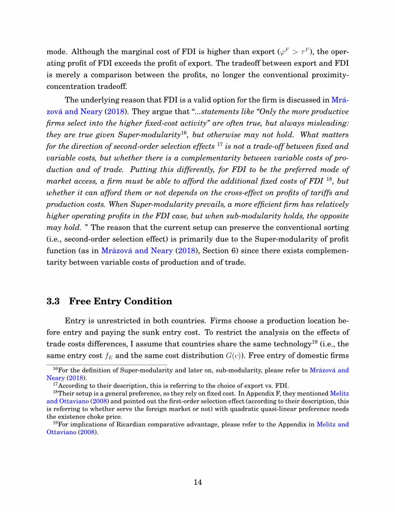
For illustration purpose, I plotted the optimal non-cooperative tariff level com-puted from equation (35) as a function of ϕ and α35 . For k = 1, the Nash tariff withoutFDI (indicated in green color) and the Nash tariff with FDI (indicated in blue color)are plotted as follow :

Figure 4: Three-dimensional Nash Tariff with k = 1

The yellow plane separates the space. The area above indicates no FDI activitysince ϕ < tτ and the area below indicates FDI occurs since ϕ > tτ . The red planeindicates zero net tariff, i.e. t = 1 since α is chosen such that the optimal tariff whenFDI occurs is greater than 1. Then it makes sense that the blue plane lies in betweenyellow plane and the red plane. Several observations stand out from the graph:

• As stated in Proposition 3, Nash tariff without FDI is always higher than theNash tariff with FDI. This confirms the finding in Cole and Davies (2011). Thegain from implementing tariff is smaller due to the tariff-jumping multination-als who lower the tariff base. This can be seen from Figure 2, where the massof foreign exporters is reduced due to the decrease of exporter cutoff and theincrease of multinational cutoff.

• ϕ does not affect the Nash tariff level without FDI since when FDI is not anoption, ϕ does not affect any exporter behavior. However, according to the Figure

35Again, here α is chosen to be larger than 2cD so that the optimal tariff level will be greater than 1.

33

4 in Cole and Davies (2011), the fixed cost parameter (λ) affects the Nash tarifflevel without FDI, as well as with FDI. This is because, in their setup, both thefixed costs of export and FDI are affected by λ. Hence the change of λ will havea direct impact on the incentive to implement tariff. In the current setup, thechange in ϕ will only affect the tariff level when FDI occurs.

• As ϕ increases, the Nash tariff with FDI is increasing, and it is getting closerto the Nash Tariff without FDI. One one hand, if ϕ approaches infinity, thenthe FDI cutoff will be zero, indicating foreign firms only excess home countryvia exports. Hence the Nash tariff level returns to the Nash tariff without FDIcase. On the other hand, when FDI is an option, Nash tariff level is increasingin ϕ. This is similar to the results in Cole and Davies (2011) regarding λ, thehigher ϕ reduces the cutoff of multinational (cFDI), making the least productivemultinationals to become exporters, increasing the tariff base, hence increasingthe incentive of imposing a higher tariff.

• For high ϕ, the Nash tariff level (indicated by blue plane) lies below the yel-low plane, indicating FDI will occur in equilibrium, confirming the finding inCole and Davies (2011). As can be seen from the two-dimensional graph below,the bold line indicates the country’s choice of Nash tariff. Same with Cole andDavies, the corner solution exists:

Figure 5: Two-dimensional Nash Tariff

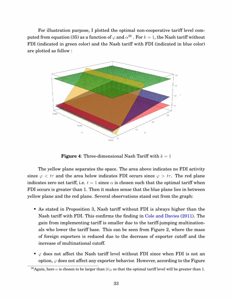
• Different from Cole and Davies (2011), in the current setup, we can see how thecompetitive environment affects the Nash tariff choice of the policymaker. Forillustration purpose, I contrast the following two cases: k = 1 and k = 1.05.

34

Figure 6: Three-dimensional Nash Tariff for k = 1.05 (left) and k = 1 (right)

According to discussion in Section 6.2, with the current quadratic quasi-linearpreference, the market equilibrium tends to undersupplies varieties from firms withhigher productivity/lower marginal cost, and oversupplies varieties from firms withlower productivity/higher marginal cost. The degree of firm heterogeneity affects thechoice of noncooperative tariff level. Here, I will briefly highlight the role of firmheterogeneity and its interplay with FDI under variable markup. More intuition willbe discussed in Section 6.2.

• Nash tariff without FDI (k = 1) > Nash tariff without FDI (k = 1.05). Whenk goes from 1 to 1.05, this tends to foster the under-provision of variety in themarket equilibrium. One can show that the number of varieties in the marketoutcome is decreasing in k36. Together with the fact that demand for differenti-ated varieties is sufficiently high, this explains why Nash tariff (k = 1) > Nashtariff (k = 1.05). When k = 1, there is relatively more varieties in the economy,the economic environment is "too competitive". This gives the policymaker an in-centive to increase tariff to deter entry, hence improving welfare. When k = 1.05,the market provides relatively fewer varieties in the economy, the policy makerhas smaller incentive to deter entry. Hence the tariff level is lower. In contrast,Cole and Davies (2011) are not able to discuss the role of firm heterogeneityand its impact on Nash tariff. This is due to their specific variety/productivityassumption37 and the fact that under CES and monopolistic competition, firmheterogeneity does not create any externality in the economy. While this makes

36See Appendix37See their footnote 11.

35

their presentation simple and neat, it also removes the possibility to study theimpact of competitive environment (through the interaction of quadratic quasi-linear preference and productivity distribution) on Nash tariff.

• Nash tariff with FDI (k = 1, green) < Nash tariff with FDI (k = 1.05, blue).According to the discussion in Section 5.1 and 5.3, the presence of FDI can po-tentially reduce misallocation. In the following graph, I use k = 1 (the greenplane) to represent an economy with larger misallocation and k = 1.05 (blueplane) to represent an economy with smaller misallocation. When the misallo-cation is large (k = 1), the Nash tariff with FDI is lower compared to the casewhen misallocation is small (k = 1.05). This is due to the reduction of misalloca-tion triggered by tariff change in the presence of tariff-jumping FDI.

Figure 7: Nash Tariff with FDI when k = 1.05 (blue) and k = 1 (green)

6 Role of Variable Markup

This section further investigates the role of variable markup in the current setup.I first study how would a change in ad valorem tariff affect the covariance betweenfirm-level markup and change in firm-level employment share, which is crucial instudying the pro-competitive effect of trade in Arkolakis et al. (2018). I also investi-gate the impact of FDI on this covariance. Then I study how would a change in advalorem tariff affect the average markup distribution.

36

6.1 Misallocation

According to Arkolakis et al. (2018), variable markups can create a new source of gainor loss from trade liberalization, depending on whether low-cost firms, which chargehigh markups and under-supply their varieties, end up growing in size. Accordingto their Appendix A.4, the effect of trade liberalization on the welfare of country j

depends on the sign of the covariance of the markup, charged by a firm in country jthat produces variety for market i, and a change in its labor share that is needed toproduce this variety for this market:

cov(mi (ω) ,

dli (ω)

Lj

)(37)

where li(ω) is the total employment associated with a production of variety ω in coun-try j for sales in country i. In other words, if this covariance is positive, then tradeliberalization has an additional positive effect on welfare in country j through a reduc-tion in misallocation. In their setup, without considering the choice of FDI, equation(37) becomes:

cov(mi (ω) ,

dli (ω)

Lj

)= NH

D

∫ cHD

0

pHD (c)

c

d[cqHD (c)

]LH

dG (c)

G (cHD)

+NHX

∫ cHX

0

pHX (c)

τF c

d[cτF qHX (c)

]LH

dG (c)

G (cHX)

It is important to notice that this covariance is at the firm-level. Therefore it not onlyincludes firm’s domestic production decision but also relates to its export decision. Intheir setting, this covariance is negative, so the presence of variable markups reducesthe welfare gain from trade. This is because a decrease in trade costs makes exportingfirms relatively more productive, which leads to changes in markups. When demandis log-concave, as assumed in Krugman (1979), higher markups implies incompletepass-through of changes in marginal costs to prices, which tends to lower the welfaregains from trade.

37

In the current setup, the covariance term is:

cov(mi (ω) ,

dli (ω)

Lj

)= NH

D

∫ cHD

0

pHD (c)

c

d[cqHD (c)

]LH

dG (c)

G (cHD)

+NHX

∫ cHX

cHFDI

pHX (c)

τF c

d[cτF qHX (c)

]LH

dG (c)

G (cHX)

+NHFDI

∫ cHFDI

0

pHFDI (c)

ϕF c

d[cϕF qHFDI (c)

]LH

dG (c)

G (cHFDI)

Several differences compared to Arkolakis et al. (2018): (1) trade liberalization canalso take the form of tariff reduction, generating pro-competitive effect; (2) the covari-ance has an additional item due to the choice of FDI, which means now the welfareimplication of a change in tariff also depends on firm’s FDI activity. In Appendix A.11,I analytically derived the covariance term under symmetry:

cov(mi (ω) ,

dli (ω)

Lj

)=

(α− cD) dcD2η (1 + t−kτ−k)

2k + 1 +

[(tτ)−k − ξk

]×[2k + 1− k (1− tτξ) (tτξ)k − (tτξ)k

]+ ξk (k + kϕ+ 1)

Since dcD/dt > 038, that means for dt > 0, the covariance term is positive, indicatinga reduction in misallocation through protection. As discussed in Section 4, whenα > 2cD, demand for the differentiated varieties is sufficiently high, the optimal tariffunder this case is greater than one, which means an increase in tariff raises thewelfare. The presence of variable markup and FDI results in a positive covarianceterm between firm-level markup and change in firm-level employment share, whichmeans the gain from protection, in this case, is even larger due to the reduction inmisallocation. Since the current quadratic quasi-linear preference satisfies the basicassumptions39 in the general demand structure in Arkolakis et al. (2018), that meansan increase in tariff will decrease the relative demand for high-cost varieties. This, inturn, triggers a reallocation of labor away from these goods. Intuitively, the changein tariff induces tariff-jumping in the economy, triggering labor reallocation towardthe multinationals, whose goods are originally under-supplied and who charge highermarkups. Misallocation is reduced since the market becomes more concentrated afterthe change in tariff. Therefore, generating a positive correlation between markupsand the labor share, hence increase the gains from the change in tariff.

38See Appendix A.1139See their 2012 working paper, Section 5.

38

6.2 Social Optimum vs. Market Outcome

To further understand the role of variable markup and its impact on tariff choice, Ifollow Nocco et al. (2014) to study the social optimum in the current economy. Sincequadratic quasi-linear utility implies transferable utility, social welfare may be ex-pressed as the sum of all consumers’ utilities. The planner chooses the number ofentrants (NH

E , NFE ) and output level (qH0 , qF0 , qHi , qFi ) to achieve the first-best outcome40:

maxNE ,q0,qi

W

s.t. qH0 + qF0 + f(NHE +NF

E

)+NH

E

∫ cM

0

[cqHD (c) + τF cqHX (c) + ϕF cqHFDI (c)

]dG (c)

+NFE

∫ cM

0

[cqFD (c) + τHcqFX (c) + ϕHcqFFDI (c)

]dG (c) = 2 + qH0 + qF0

Compared to the social optimum, the market outcome produces multiple failures: (1)the home domestic market selection is weaker than the socially optimum selection(cHMD > cHOD

), (2) the home exporter market selection is weaker than the socially opti-

mum selection(cHMX > cHOX

), (3) the home FDI market selection is stronger than the

socially optimum selection(cHMFDI < cHOFDI

), (4) market outcome undersupplies varieties

with low marginal production cost41, qHMD < qHOD when c <[2− (2/4)1/(k+2)

]cHOD , (5)

depending on the relative demand for the differentiated varieties, the market out-come does not always yield the socially optimal level of the total number of varieties(NH , NF ) and the number of entrants (NH

E , NFE ).

The inefficiencies in the market outcome originate from multiple externalitiesin the economy. The monopoly power in the differentiated-good sector allow a firmto price over its marginal cost, under the free-entry condition, this externality tendsto create too many varieties. The new entrant will also cut the profits of existingfirms, and this business-stealing effect also tends to create too many varieties. Withquadratic quasi-linear preference, the consumers display “love of variety”, yet firmsdo not consider this fact when making entry decision. This tends to create not enoughvarieties in the economy. With variable markup, firm heterogeneity also creates anexternality. Since markup is decreasing in marginal cost, this results in the lowmarginal cost firms (more productive) being inefficiently small and high marginal

40For detailed solution of first-best outcome, please refer to the Appendix.41Please refer to the Appendix for a detailed expression of 4.

39

cost firms (less productive) being inefficiently large in the market outcome. All theseexternalities work together to generate market failures in the current economy.

According to Dhingra and Morrow (2012), when monopolistic competition is com-bined with CES preference, the market outcome coincides with the first-best outcome.The externalities mentioned above exactly cancel with each other42. The current econ-omy deviates from this benchmark due to the quadratic quasi-linear preference. Theforces that generate externality do not cancel with each other. The market outcomedoes not coincide with the first-best outcome.

More importantly, entry in the current economy is not socially optimal as inMelitz (2003); Melitz and Ottaviano (2008). According to Arkolakis et al. (2012), entrylevel is not affected by the change in transportation cost due to one of their “macro”assumptions-aggregate profits in any country is a constant share of aggregate rev-enue, which is satisfied in the special case of a Pareto distribution on productivitydraws. Balistreri et al. (2011) were the first to notice that entry43 is no longer fixedif ad valorem tariff is introduced. In the current framework, based on equation (26),entry is affected by the tariff level. An increase in home tariff can bring the marketoutcome closer to the unconstrained optimum:

Figure 8: Cutoff responses to an increase in tH

When the relative demand for the differentiated varieties is sufficiently high,the social planner has an incentive to encourage protection since it can bring all the

42Note, firm heterogeneity does not create externality since all firms charge identical markup43For a detailed discussion of entry in heterogeneous firm framework, see Caliendo et al. (2017).

However, in Cole and Davies (2011), although ad valorem tariff is introduced, the entry margin isentirely ignored. This is likely due to the fact that they do not obtain a closed-form solution of themodel.

40

cutoffs closer to their first-best level, reducing the misallocation in the economy. Thisis because a higher tariff will reduce the markup of all the firms, but disproportionallythose firms charge higher markups, causing these firms to pass their cost advantageto prices.

Turning back to the results in Section 5.4, where the uncooperative tariff leveldepends on the shape of Pareto distribution k, the degree of firm-heterogeneity de-creases as k increases. If k → ∞, the marginal cost distribution becomes degenerateat its lower bound cM , firm heterogeneity reaches zero, and all the firms have identi-cal marginal cost draw. As k decreases, the degree of firm heterogeneity increases. Ifk → 0, the marginal cost distribution becomes uniform distribution over [0, cM ], firmheterogeneity reaches maximum since firms have equal chance to draw any marginalcost level over the support. If k is small, which means there are relatively moreproductive firms in the economy, since tariff-jumping FDI happens among the moreproductive firms (exporters and FDI firms) along the marginal cost distribution, thereduction of misallocation has a more substantial impact on the economy. If k is large,which means there are relatively less productive firms in the economy, the reductionof misallocation through tariff-jumping has a smaller impact on the economy. In Sec-tion 5.4, I find Nash tariff without FDI (small k) > Nash tariff without FDI (big k) andNash tariff with FDI (small k) < Nash tariff with FDI (big k), this shows under thevariable markup, the degree of firm heterogeneity affects the choice noncooperativelevel. When the economy features a higher degree of firm heterogeneity (small k),allowing firms to engage in FDI can lower the tariff competition by reducing misallo-cation.

7 Conclusion

In this paper, I study the trade policy implication of revenue tariffs with rebates toconsumers in the presence of variable markups and firm’s endogenous choice to en-gage in multinational production. I introduced ad valorem tariff and horizontal FDIinto the Melitz and Ottaviano (2008) framework. My conclusions can be broadly sum-marized as follows. First, I find protectionist trade policy can create pro-competitiveeffect if the increase of tariff-jumping multinationals dominates the reduction of for-eign exporters. Second, I find that in contrast to Cole and Davies (2011), the welfareimplication of protectionist tariffs crucially depends on consumer’s preference. If thedemand for the differentiated varieties is sufficiently high, this will drive excess firm

41

entry. The business-stealing effect and substitution effect will dominate the positiveimpact on consumers generated through the entry, creating negative externality inthe economy. In this case, the social planner can improve the welfare by properlydeterring entry through tariff. Third, complementing the results in Arkolakis et al.(2018), I find a change in ad valorem tariff can affect the degree of misallocation inthe economy by reallocating labor toward the the more productive firms, hence affect-ing the choice of Nash tariff choice. Lastly, the presence of FDI affects a country’snon-cooperative tariff choice. In particular, it can reduce the non-cooperative tariffthrough a novel channel: reducing the degree of misallocation in the economy.

Given these results, there are several potential avenues for future research. Forexample, deviating from Pareto distribution. As discussed by Feenstra (2018), if thesupport of cost distribution become bounded, other channels that will affect the pro-competitive effect of trade will begin to work, delivering different welfare implicationof trade. On the other hand, the combination of Melitz and Pareto implies that tradecost will only affect export through extensive margin, but this is at odds with theempirical fact that most of the adjustments happen along the intensive margin. Thiscan be reconciled by introducing log-normal distribution44.

Another interesting path would be to investigate if the current trade policy re-sults still hold under alternative demand structures that generate variable markups.Several approaches are being considered: (1) Deviating from CES and quadraticquasi-linear preference. For instance, QMOR (quadratic mean of order r) preferenceas in Feenstra (2018). This preference nested CES and the Melitz and Ottaviano(2008) preference. Incorporating ad valorem tariff and FDI into this framework willprovide a direct comparison of the Nash tariff level under these two special cases.Other preferences include IA (indirectly additive) preference as in Bertoletti et al.(2018), AQS (additively quasi-separable) preference as in Behrens and Murata (2007),and translog preference as in Rodriguez-Lopez (2011). (2) Dropping the monopolisticcompetition in Cole and Davies (2011), this will generate variable markups under theCES preference and can also allow comparison the Nash tariff level (at least numer-ically). For example, by assuming Bertrand or Cournot competition, as in Bernardet al. (2003), Atkeson and Burstein (2008), and Edmond et al. (2015).

Lastly, the trade policy implication here is primarily focusing on the monopo-listically competitive sector. It would be interesting and relevant to see how woulda multi-sector framework affects the policy results. For example, Spearot (2016) ex-

44See Fernandes et al. (2017) for a detailed discussion

42

tended Melitz and Ottaviano (2008) by incorporating multiple countries and multi-ple industries with heterogeneity in the country-by-industry shape parameters of thePareto cost distributions and provided quantitative implication for unilateral tariffliberalization. The excess entry in the current framework might have different im-plication here since the mass of entrants in a particular sector now depends on therelative expenses on goods produced there. I leave these questions for future work.

43

References

ALFARO, L. AND M. CHEN (2018): “Transportation Cost and the Geography of For-eign Investment,” Handbook of International Trade and Transportation.

ALFARO, L. AND M. X. CHEN (2015): “Multinational Activity and Information andCommunication Technology,” World Development Report.

ANTRÀS, P. AND S. R. YEAPLE (2014): “Multinational firms and the structure ofinternational trade,” Handbook of International Economics, 4, 55–130.

ARKOLAKIS, C., A. COSTINOT, D. DONALDSON, AND A. RODRÍGUEZ-CLARE (2018):“The elusive pro-competitive effects of trade,” The Review of Economic Studies.

ARKOLAKIS, C., A. COSTINOT, AND A. RODRIGUEZ-CLARE (2012): “New trade mod-els, same old gains?” American Economic Review, 102, 94–130.

ASKER, J., A. COLLARD-WEXLER, AND J. DE LOECKER (2017): “Market Power andProduction (Mis) Allocation. A Study of the World Oil Market,” Mimeo, PrincetonUniversity.

ATKESON, A. AND A. BURSTEIN (2008): “Pricing-to-market, trade costs, and interna-tional relative prices,” American Economic Review, 98, 1998–2031.

BAGWELL, K. AND S. H. LEE (2015): “Trade policy under monopolistic competitionwith firm selection,” Mimeogr., Stanford University.

BALDWIN, R., R. FORSLID, P. MARTIN, AND G. OTTAVIANO (2003): “F. Robert-Nicoud (2003),” Economic Geography and Public Policy.

BALISTRERI, E. J., R. H. HILLBERRY, AND T. F. RUTHERFORD (2011): “Structuralestimation and solution of international trade models with heterogeneous firms,”Journal of international Economics, 83, 95–108.

BARRELL, R. AND N. PAIN (1999): “Trade restraints and Japanese direct investmentflows,” European Economic Review, 43, 29–45.

BEHRENS, K., G. MION, Y. MURATA, AND J. SUEDEKUM (2018): “Quantifying theGap between Equilibrium and Optimum Under Monopolistic Competition,” CEPRDP 11642.

44

BEHRENS, K., G. MION, AND G. I. OTTAVIANO (2011): “Economic integration andindustry reallocations: some theory with numbers,” International Handbook on theEconomics of Integration: Competition, Spatial Location of Economic Activity andFinancial Issues, 2, 169.

BEHRENS, K. AND Y. MURATA (2007): “General equilibrium models of monopolisticcompetition: a new approach,” Journal of Economic Theory, 136, 776–787.

BELDERBOS, R., H. VANDENBUSSCHE, AND R. VEUGELERS (2004): “Antidumpingduties, undertakings, and foreign direct investment in the EU,” European EconomicReview, 48, 429–453.

BERNARD, A. B., J. EATON, J. B. JENSEN, AND S. KORTUM (2003): “Plants andproductivity in international trade,” American Economic Review, 93, 1268–1290.

BERTOLETTI, P., F. ETRO, AND I. SIMONOVSKA (2018): “International Trade withIndirect Additivity,” American Economic Journal: Microeconomics.

BHAGWATI, J. N. (1969): The Generalized Theory of Distortions and Welfare, Cam-bridge, MIT.

BLONIGEN, B. A. (2002): “Tariff-jumping antidumping duties,” Journal of interna-tional Economics, 57, 31–49.

BLONIGEN, B. A. AND R. C. FEENSTRA (1997): “Protectionist threats and foreigndirect investment,” in The effects of US trade protection and promotion policies,University of Chicago Press, 55–80.

BLONIGEN, B. A., K. TOMLIN, AND W. W. WILSON (2004): “Tariff-jumping FDI anddomestic firm’s profits,” Canadian Journal of Economics, 37, 656–677.

BRAINARD, S. L. (1997): “An empirical assessment of the proximity-concentrationtradeoff between multinational sales and trade,” American Economic Review, 87,520–544.

BRECHER, R. A. AND C. F. D. ALEJANDRO (1977): “Tariffs, foreign capital and im-miserizing growth,” Journal of international Economics, 7, 317–322.

CALIENDO, L., R. C. FEENSTRA, J. ROMALIS, AND A. M. TAYLOR (2017): “Tariff re-ductions, entry, and welfare: Theory and evidence for the last two decades,” NBERWorking Paper, 21768.

45

CEA (2016): “Benefits of Competition and Indicators of Market Power,” Council ofEconomic Advisers Issue Brief, April 2016.

COLE, M. T. AND R. B. DAVIES (2011): “Strategic tariffs, tariff jumping, and hetero-geneous firms,” European Economic Review, 55, 480–496.

CONYON, M. J., S. GIRMA, S. THOMPSON, AND P. W. WRIGHT (2002): “The produc-tivity and wage effects of foreign acquisition in the United Kingdom,” The Journalof Industrial Economics, 50, 85–102.

COSTINOT, A., A. RODRÍGUEZ-CLARE, AND I. WERNING (2016): “Micro to macro:Optimal trade policy with firm heterogeneity,” Tech. rep., National Bureau of Eco-nomic Research.

DE LOECKER, J. AND J. EECKHOUT (2017): “The rise of market power and themacroeconomic implications,” Tech. rep., National Bureau of Economic Research.

DE LOECKER, J., P. K. GOLDBERG, A. K. KHANDELWAL, AND N. PAVCNIK (2016):“Prices, markups, and trade reform,” Econometrica, 84, 445–510.

DEMIDOVA, S. (2017): “Trade policies, firm heterogeneity, and variable markups,”Journal of International Economics, 108, 260–273.

DEMIDOVA, S. AND A. RODRIGUEZ-CLARE (2009): “Trade policy under firm-levelheterogeneity in a small economy,” Journal of International Economics, 78, 100–112.

DHINGRA, S. AND J. MORROW (2012): “Monopolistic competition and optimum prod-uct diversity under firm heterogeneity,” London School of Economics, mimeograph.

DOMS, M. E. AND J. B. JENSEN (1998): “Comparing wages, skills, and productiv-ity between domestically and foreign-owned manufacturing establishments in theUnited States,” in Geography and ownership as bases for economic accounting, Uni-versity of Chicago Press, 235–258.

EDMOND, C., V. MIDRIGAN, AND D. Y. XU (2015): “Competition, markups, and thegains from international trade,” American Economic Review, 105, 3183–3221.

FEENSTRA, R. C. (2018): “Restoring the product variety and pro-competitive gainsfrom trade with heterogeneous firms and bounded productivity,” Journal of Inter-national Economics, 110, 16–27.

46

FELBERMAYR, G., B. JUNG, AND M. LARCH (2013): “Optimal tariffs, retaliation,and the welfare loss from tariff wars in the Melitz model,” Journal of InternationalEconomics, 89, 13–25.

FERNANDES, A., P. KLENOW, M. D. PIEROLA, A. RODRIGUEZ-CLARE, AND

S. MELESHCHUK (2017): “The Intensive Margin in Trade,” .

HELPMAN, E. AND P. R. KRUGMAN (1989): Trade Policy and Market Structure, MITpress.

HELPMAN, E., M. J. MELITZ, AND S. R. YEAPLE (2004): “Export versus FDI withheterogeneous firms,” American Economic Review, 94, 300–316.

HIJZEN, A., H. GÖRG, AND M. MANCHIN (2008): “Cross-border mergers and acqui-sitions and the role of trade costs,” European Economic Review, 52, 849–866.

IRARRAZABAL, A., A. MOXNES, AND L. D. OPROMOLLA (2013): “The margins ofmultinational production and the role of intrafirm trade,” Journal of Political Econ-omy, 121, 74–126.

KELLER, W. AND S. R. YEAPLE (2008): “Global production and trade in the knowl-edge economy,” Tech. rep., National Bureau of Economic Research.

KRUGMAN, P. R. (1979): “Increasing returns, monopolistic competition, and interna-tional trade,” Journal of international Economics, 9, 469–479.

MANKIW, N. G. AND M. D. WHINSTON (1986): “Free entry and social inefficiency,”The RAND Journal of Economics, 48–58.

MATALONI, R. J. (2011): “The productivity advantage and global scope of US multi-national firms,” BEA Working Paper,WP2011-02.

MELITZ, M. (2003): “The Impact of Trade on Intra-Industry Reallocations and Aggre-gate Industry Productivity,” Econometrica, 71, 1695–1725.

MELITZ, M. AND G. OTTAVIANO (2008): “Market Size, Trade, and Productivity,” Re-view of Economic Studies, 75.

MRÁZOVÁ, M. AND J. P. NEARY (2018): “Selection Effects with HeterogeneousFirms,” Journal of the European Economic Association, jvy024.

NOCCO, A., G. I. OTTAVIANO, AND M. SALTO (2014): “Monopolistic competition andoptimum product selection,” American Economic Review, 104, 304–09.

47

OTTAVIANO, G., T. TABUCHI, AND J.-F. THISSE (2002): “Agglomeration and traderevisited,” International Economic Review, 409–435.

PIETROVITO, F., A. F. POZZOLO, AND L. SALVATICI (2013): “Exports versus ForeignDirect Investments: Evidence from Cross-Country Industry Data,” Firms in theInternational Economy: Firm Heterogeneity Meets International Business, 55.

RAMONDO, N. AND A. RODRÍGUEZ-CLARE (2013): “Trade, multinational production,and the gains from openness,” Journal of Political Economy, 121, 273–322.

RODRIGUEZ-LOPEZ, J. A. (2011): “Prices and exchange rates: A theory of disconnect,”The Review of Economic Studies, 78, 1135–1177.

SPEAROT, A. (2016): “Unpacking the Long-Run Effects of Tariff Shocks: New Struc-tural Implications from Firm Heterogeneity Models,” American Economic Journal:Microeconomics, 8, 128–67.

VENABLES, A. J. (1985): “Trade and trade policy with imperfect competition: Thecase of identical products and free entry,” Journal of International Economics, 19,1–19.

WEINBERGER, A. (2015): “Markups and misallocation with trade and heterogeneousfirms,” FRB Dallas Globalization and Monetary Policy Institute Working Paper No.251.

48

A Proofs

A.1 Proof of Lemma 1

To prove this Lemma, I first prove the following condition:

Φl1 + Φl

2 > ψl ∈ (0, 1) for l ∈ H,F

Given ψl ≡(τ l)−k (

tl)−(k+1) and

Φl1 ≡

(k + 1) (k + 2) tl(τ l)2

2

(1

tlτ l

)k+2

−(

1

tlτ l

)2 (ξl)k

− 2k

k + 1

[(1

tlτ l

)k+2

−(

1

tlτ l

)(ξl)k+1

]+

k

k + 2

[(1

tlτ l

)k+2

−(ξl)k+2

]

Φl2 ≡

(k + 1) (k + 2)(ξl)k

2

[1− 2kϕlξl

k + 1+k(ϕlξl

)2

k + 2

]

It is then straightforward to show

Φl1 + Φl

2 = ψl +(k + 1) (k + 2)

(ξl)k

2

(1− 1

tl

)− 2k

k + 1ξl(ϕl − τ l

)+

k

k + 2

(ξl)2((ϕl)2 − tl

(τ l)2)

To show that Φl1 + Φl

2 > ψl, it is equivalent to show that(1− 1

tl

)− 2k

k + 1ξl(ϕl − τ l

)+

k

k + 2

(ξl)2((ϕl)2 − tl

(τ l)2)> 0

Based on the definition of ξl ≡(√

tl − 1)/(√

tlϕl − tlτ l)

, the above equation be-

49

comes:(1− 1

tl

)− 2k

k + 1

√tl − 1√

tlϕl − tlτ l(ϕl − τ l

)+

k

k + 2

( √tl − 1√

tlϕl − tlτ l

)2 ((ϕl)2 − tl

(τ l)2)> 0

⇔(

1− 1

tl

)+

k

k + 2

( √tl − 1√

tlϕl − tlτ l

)2 ((ϕl)2 − tl

(τ l)2)>

2k

k + 1

√tl − 1√

tlϕl − tlτ l(ϕl − τ l

)

⇔tl − 1

tl+

k

k + 2

(√tl − 1

)2

tlϕl +

√tlτ l

ϕl −√tlτ l

>2k

k + 1

√tl − 1√tl

ϕl − τ l

ϕl −√tlτ l

⇔tl − 1

tl+

k

k + 2

(√tl − 1

)2

tlϕl +

√tlτ l

ϕl −√tlτ l

>2k

k + 1

√tl − 1√tl

ϕl − τ l

ϕl −√tlτ l

Multiply both sides by (k + 1) (k + 2) tl(ϕl −

√tlτ l)

, I have

(k2 + 3k + 2

) (√tl + 1

)(ϕl −

√tlτ l)

+(k2 + k

) (√tl − 1

)(ϕl +

√tlτ l)>(2k2 + 4k

)√tl(ϕl − τ l

)⇔2√tlϕl − 2

√tlτ l + 2 (k + 1)

(ϕl − tlτ l

)> 0

⇔2√tl(ϕl − τ l

)+ 2 (k + 1)

(ϕl − tlτ l

)> 0

This is obviously true when ϕl > tlτ l (note tl > 1), which is the assumption wemade to guarantee the existence of tariff-jumping FDI.

Compare the cutoff expressions, for l ∈ H,F

Open economy, with tariff, export and FDI: cHD1 =

[γφ

1−(ΦF

1 + ΦF2

)1− (ΦF

1 + ΦF2 ) (ΦH

1 + ΦH2 )

] 1k+2

Open economy, with tariff and export: cHD2 =

(γφ

1− ψF

1− ψFψH

) 1k+2

, ψl =(τ l)−k (

tl)−(k+1)

Closed economy: cHD3 = (γφ)1

k+2 , as in MO(2008) Section 2

With the proved condition, it is straightforward to show that

cHD3 > cHD2 > cHD1

50

A.2 Proof of Lemma 2

Based on the solution of cHD =

[γφ

1−(ΦF

1 + ΦF2

)1− (ΦF

1 + ΦF2 ) (ΦH

1 + ΦH2 )

] 1k+2

, I have

∂cHD∂tH

=γφ

k + 2

[γφ

1−(ΦF

1 + ΦF2

)1− (ΦF

1 + ΦF2 ) (ΦH

1 + ΦH2 )

]− k+1k+2(ΦF

1 + ΦF2

) [1−

(ΦF

1 + ΦF2

)][1− (ΦF

1 + ΦF2 ) (ΦH

1 + ΦH2 )]

2

∂(ΦH

1 + ΦH2

)∂tH

=1

k + 2cHD

(ΦF

1 + ΦF2

)1− (ΦF

1 + ΦF2 ) (ΦH

1 + ΦH2 )︸ ︷︷ ︸

>0

∂(ΦH

1 + ΦH2

)∂tH

So the sign crucially depends on∂(ΦH

1 + ΦH2

)∂tH

. It is straightforward to show that

∂(ΦH

1 + ΦH2

)∂tH

= − k + 1

2tH(√

tHϕH − tHτH)2

2

(tHτH)k

[tH(τH)2 − 2ϕH

√tHτH +

(ϕH)2]

+(ξH)k [−2tH

(τH)2 − 2k

√tHtH

(τH)2

+ k(tHτH

)2

+2 (k + 2)√tHτHϕH − (k + 2)

(ϕH)2]

= − k + 1

2tH(√

tHϕH − tHτH)2

︸ ︷︷ ︸<0

2(ϕH −

√tHτH

)2 [(tHτH

)−k − (ξH)k]

−(ξH)kk(ϕH − tHτH

) (ϕH + tHτH − 2

√tHτH

)The expression within the big bracket is greater than zero for all k ∈ [1,+∞)

when ϕH > tHτH , to see this, it is equivalent to show

2(ϕH −

√tHτH

)2 [(tHτH

)−k − (ξH)k] > (ξH)k k (ϕH − tHτH) (ϕH + tHτH − 2√tHτH

)

51

For k = 1, the expression become

2(ϕH −

√tHτH

)2[

1

(tHτH)− ξH

]> ξH

(ϕH − tHτH

) (ϕH + tHτH − 2

√tHτH

)⇔2

(ϕH −

√tHτH

)2(

1

ξHtHτH− 1

)>(ϕH − tHτH

) (ϕH + tHτH − 2

√tHτH

)⇔2

(ϕH −

√tHτH

)2 ϕH − tHτH√tHτH

(√tH − 1

) > (ϕH − tHτH) (ϕH + tHτH − 2√tHτH

)⇔2

(ϕH −

√tHτH

)2

>√tHτH

(√tH − 1

)(ϕH + tHτH − 2

√tHτH

)⇔2

(ϕH)2 − 3

√tHτHϕH + 3

√tHtH

(τH)2 − tHτHϕH −

(tHτH

)2> 0

⇔(ϕH − tHτH

) (2ϕH + tHτH − 3

√tHτH

)> 0

which is obviously true.

For k approach infinity, to prove the equation, it is equivalent to show

2(ϕH −

√tHτH

)2

(ϕH − tHτH)(ϕH + tHτH − 2

√tHτH

) > k

(ξHtHτH)−k − 1

As k →∞, the limit of right-hand side is 0. It means as long as the left-hand sideis positive, the equation is true for k → ∞. The left hand side is obviously positivegiven ϕH > tHτH . Therefore,

∂(ΦH

1 + ΦH2

)∂tH

< 0⇒ ∂cHD∂tH

< 0

To show∂cFD∂tH

is easier, note that

∂cFD∂tH

=

[γφ

1−(ΦH

1 + ΦH2

)1− (ΦF

1 + ΦF2 ) (ΦH

1 + ΦH2 )

]− k+1k+2 γφ

[1−

(ΦF

1 + ΦF2

)]/ (k + 2)

[1− (ΦF1 + ΦF

2 ) (ΦH1 + ΦH

2 )]2

−∂(ΦH

1 + ΦH2

)∂tH

=cFDk + 2

[1−

(ΦF

1 + ΦF2

)][1− (ΦF

1 + ΦF2 ) (ΦH

1 + ΦH2 )] [1− (ΦH

1 + ΦH2 )]︸ ︷︷ ︸

>0

−∂(ΦH

1 + ΦH2

)∂tH︸ ︷︷ ︸>0

> 0

52

A.3 Proof of Lemma 3

Based on the cutoff relations, it is straightforward to show

∂cHX∂tH

=∂(cFD/t

F τF)

∂tH=

1

tF τF∂cFD∂tH

> 0

∂cFX∂tH

=∂(cHD/t

HτH)

∂tH=

1

(tH)2 τH

(∂cHD∂tH

tH − cHD)

To show∂cHD∂tH

tH − cHD < 0 is equivalent to show

1

k + 2cHD

(ΦF

1 + ΦF2

)1− (ΦF

1 + ΦF2 ) (ΦH

1 + ΦH2 )

∂(ΦH

1 + ΦH2

)∂tH

tH < cHD

⇔ 1

k + 2

(ΦF

1 + ΦF2

)1− (ΦF

1 + ΦF2 ) (ΦH

1 + ΦH2 )︸ ︷︷ ︸

>0

∂(ΦH

1 + ΦH2

)∂tH

tH︸ ︷︷ ︸<0

< 1

Which is obviously true. Therefore, Lemma 3 is proved.

A.4 Proof of Lemma 4

This part is not easy to prove, notice

∂cFFDI∂tH

=∂(cHDξ

H)

∂tH=∂cHD∂tH

ξH +∂ξH

∂tHcHD

=cHDξ

H

k + 2

(ΦF

1 + ΦF2

)1− (ΦF

1 + ΦF2 ) (ΦH

1 + ΦH2 )︸ ︷︷ ︸

>0

∂(ΦH

1 + ΦH2

)∂tH︸ ︷︷ ︸<0

+∂ξH

∂tHcHD︸ ︷︷ ︸

>0

It is straightforward to verify that under the parameter choice in Section 4.3,the second term dominates the first term, so foreign country’s FDI cutoff level (cFFDI)isstrictly increasing as Home country’s tariff (tH) increases. Do notice, the other choiceof ξ, which is ξ =

(√t+ 1

)/(√

tϕ+ tτ)

will make the second item negative, therebymaking cFFDI decreasing in response to tH ’s increase, hence no tariff jumping.

53

A.5 Proof of Lemma 5

Based on equation (24), it’s straightforward to show

∂NH

∂tH=

2γ (k + 1)

η

−∂cHD

∂tHcHD −

∂cHD∂tH

(α− cHD

)(cHD)

2 = −2γα (k + 1)

η (cHD)2

∂cHD∂tH

> 0

∂NF

∂tH=

2γ (k + 1)

η

−∂cFD

∂tHcFD −

∂cFD∂tH

(α− cFD

)(cFD)

2 = −2γα (k + 1)

η (cFD)2

∂cFD∂tH

< 0

Now based on equation (26), as tH increases

NFE =

2 (cM)k (k + 1) γ

η (1− δHδF )

[α− cFD(cFD)

k+1− δF α− c

HD

(cHD)k+1

]

δH decreases (hence the coefficient in front of the bracket decreases), cFD increases(the first item in the bracket decreases), cHD decreases (the second item in the bracketincreases). Hence the whole expression on the right decreases, therefore ∂NF

E /∂tH <

0. Now utilizing the free-entry condition, which is equation (25)

G(cHD)NHE +G

(cFX)NFE = NH

As tH increases, NH increases, it means the left-side also needs to increase. No-tice NF

E decreases, cFX decreases, cHD decreases, it then must be true that NHE increases.

Hence, ∂NHE /∂t

H > 0.

A.6 Proof of Proposition 1

Once again, to simplify the proof, I assume symmetry, following Appendix A.11, cD =

cHD = cFD and

NE =2γckM (k + 1) (α− cD)

η (cD)k+1 (1 + t−kτ−k)

ND =2γ (k + 1) (α− cD)

η (1 + t−kτ−k) cD

NX =2γ (k + 1) (α− cD)

η (1 + t−kτ−k) cD

[(tτ)−k − ξk

]NFDI =

2γ (k + 1) (α− cD)

η (1 + t−kτ−k) cDξk

54

Together with equation (6), (10) and (15), the average markup in (31) can bewritten as follow:

m =1

ND +NX +NFDI

[ND

∫ cD

0

mD (c)dG (c)

G (cD)

+ NX

∫ cX

cFDI

mX (c)dG (c)

G (cX)+NFDI

∫ cFDI

0

mFDI (c)dG (c)

G (cFDI)

]=

1

ND +NX +NFDI

[ND

∫ cD

0

cD + c

2c

kck−1

ckDdc

+ NX

∫ cX

cFDI

t (cX + c)

2c

kck−1

ckXdc+NFDI

∫ cFDI

0

cD + ϕHc

2ϕHc

kck−1

ckFDIdc

]=

1

ND +NX +NFDI

[ND ×

2k − 1

2k − 2+NX × t

×(

2k − 1

2k − 2− k

2k − 2(tτξ)k−1 − 1

2(tτξ)k

)+NFDI ×

(k

2k − 2

1

ϕξ+

1

2

)]

=1

1 + (tτ)−k× 2k − 1

2k − 2+t[(tτ)−k − ξk

]1 + (tτ)−k

×[

2k − 1

2k − 2− k

2k − 2(tτξ)k−1 − 1

2(tτξ)k

]+

ξk

1 + (tτ)−k×(

k

2k − 2

1

ϕξ+

1

2

)=

1

1 + (tτ)−k× 2k − 1

2k − 2︸ ︷︷ ︸weighted expected markup in domestic

+1− (tτξ)k

1 + (tτ)−k× 1

tk−1τ k

1

2

[1− (tτξ)k

]+

k

2k − 2

[1− (tτξ)k−1

]︸ ︷︷ ︸

weighted expected markup from foreign exporters

+ξk

1 + (tτ)−k×(

k

2k − 2

1

ϕξ+

1

2

)︸ ︷︷ ︸weighted expected markup from foreign FDI

A.7 Proof of Proposition 2

Proof: Based on equation (27), the social welfare can be rewritten as follow:

UH + UF = IH + IF +α− cHD

2η

(α− k + 1

k + 2cHD

)+α− cFD

2η

(α− k + 1

k + 2cFD

)Since consumer receive income from wage (which is equal to 1) and tariff rev-

55

enue, so the above equation can be rewritten as:

UH + UF = 2 +(tH − 1

)IMH +

(tF − 1

)IMF

+α− cHD

2η

(α− k + 1

k + 2cHD

)+α− cFD

2η

(α− k + 1

k + 2cFD

)

To see the welfare implication of free trade, I evaluate the first order condition ofthe above expression with respect to tariff under symmetry when tH = tF = 1. Sincesymmetry implies IMF = IMH , ∂IMF/∂tH = ∂IMH/∂tF , cFD = cHD , ∂c

FD/∂t

H = ∂cHD/∂tF ,

therefore :

∂(UH + UF

)∂t

|tH=tF =1 = (t− 1)

(∂IMH

∂tH+∂IMF

∂tH

)︸ ︷︷ ︸

~

+IMH

+2 (k + 1) cD − (2k + 3)α

2η (k + 2)

(∂cHD∂tH

+∂cFD∂tH

)

Notice, when tH = tF = 1, ~ = 0. Based on equation (26) and (28),

IMH |tH=1 = NE|tH=1 ×(cD)k+2 τ−k

2γ (k + 2) (cM)k|t=1

=2 (cM)k (k + 1) γ

(1− τ−k

)η (1− τ−2k)

(cD)k+2 τ−k

2γ (k + 2) (cM)k|t=1

=τ−k (k + 1)

η (1 + τ−k) (k + 2)(α− cD) cD|t=1

Based on the definition of ΦH and ΦF , it is straightforward to show

Φ1 + Φ2 = τ−k

Based on the proof of Lemma 2, it is straightforward to show

∂cHD∂tH

+∂cFD∂tH|t=1 =

− (k + 1) cHDτ−2k

(k + 2) (1− τ−2k)+

cFDk + 2

− (k + 1) τ−k

(1− τ−2k)

=τ−k (k + 1)

(1 + τ−k) (k + 2)cD|t=1

56

Therefore, the original first order condition can be rewritten as

∂(UH + UF

)∂t

|tH=tF =1 =τ−k (k + 1)

η (1 + τ−k) (k + 2)(α− cD) cD|t=1

+2 (k + 1) cD − (2k + 3)α

2η (k + 2)

τ−k (k + 1)

(1 + τ−k) (k + 2)cD|t=1

=τ−k (k + 1) cD

2η (k + 2)2 (1 + τ−k)[2 (k + 2) (α− cD) + 2 (k + 1) cD − (2k + 3)α]

=τ−k (k + 1) cD

2η (k + 2)2 (1 + τ−k)(α− 2cD) |t=1

Define cD ≡ cD|t=1, then this completes the proof of proposition 2.

A.8 Proof of Second-Best Social Planner Problem

Based on the definition of average consumer surplus, it can be rewritten in terms ofcD:

Avg. CS ≡ γ

2

∫ cD

0

(qD (c))2 dG (c) =(cD)k+2

4γckM (k + 1) (k + 2)> 0

Based on equation (26), under symmetry and t = 1,

NE =2γckM (k + 1) (α− cD)

η (cD)k+1 (1 + τ−k)

Then, the variety effect can be defined as the difference between consumer sur-plus and the sum of average surplus at each variety:

VE ≡ CS−NE × Avg. CS

=α− cD

2η

(α− k + 1

k + 2cD

)− 2γckM (k + 1) (α− cD)

η (cD)k+1 (1 + τ−k)× (cD)k+2

4γckM (k + 1) (k + 2)

=(α− cD)

2η

[α−

(k + 1)(1 + τ−k

)+ 1

(k + 2) (1 + τ−k)cD

]

57

The expected profit of a firm can be derived from equation (20):

π =

∫ cD

0

πD (c) dG (c) +

∫ cX

0

πX (c) dG (c)

=(cD)k+2

2γckM (k + 1) (k + 2)+

τ 2 (cX)k+2

2γckM (k + 1) (k + 2)=

(cD)k+2 (1 + τ−k)

2γckM (k + 1) (k + 2)

Notice when t = 1, cFDI = 0 and cX = cD/τ. With all these components and thefact that α > cD, equation (32) can now be properly signed:

Avg. CS =(cD)k+2

4γckM (k + 1) (k + 2)> 0

NE∂Avg. CS∂NE

=(α− cD) (cD)k+2

4γckM (k + 1) [kcD − α (k + 1)]< 0

∂VE∂NE

=(cD)k+2 2

[(k + 1)

(1 + τ−k

)+ 1]

(α− cD) + τ−kα

4γckM (k + 1) (k + 2) [α (k + 1)− kcD]> 0

NE∂π

∂NE

=(cD)k+2 (1 + τ−k

)(α− cD)

4γckM (k + 1) [kcD − (k + 1)α]< 0

Therefore, the externality of entry equals to

Avg. CS +NE∂Avg. CS∂NE

+∂VE∂NE

+NE∂π

∂NE

=

(1 + τ−k

)(cD)k+2

4γckM (k + 1) (k + 2) [kcD − (k + 1)α]︸ ︷︷ ︸<0

× (α− 2cD)

Therefore, the externality will be negative if α > 2cD, will be positive if α < 2cD.

A.9 Proof of Proposition 3

Proof: First, it is straightforward to show that ∂IMH/∂tH < 0, this is due to tariff-jumping FDI. Now compare equation (34) and (36)

58

tHS − 1 =

∂CSH

∂tH+ IMH +

∂CSF

∂tH+(tF − 1

)× ∂IMF

∂tH

−∂IMH

∂tH

tHN − 1 =

∂CSH

∂tH+ IMH

−∂IMH

∂tH

It’s straightforward to show that when α > 2cD:

∂CSF

∂tH=∂CSF

∂cFD︸ ︷︷ ︸<0

× ∂cFD

∂tH︸︷︷︸>0

< 0

(tF − 1

)× ∂IMF

∂tH=tF(tF − 1

) (τF)2

4γ (k + 2) (cM)k

[2

(1

tF τF

)k+2

− k + 2

(tF τF )2

(ξF)k

+ k(ξF)k+2

]∂NH

E

(cFD)k+2

∂tH> 0︸ ︷︷ ︸

>0

The first item indicates the distortion on F ’s consumption generated by tH , thesecond item indicates the distortion on F ’s tariff revenue generated by tH . It’s straight-forward to show the distortion on consumption is larger than the distortion on tariffrevenue. Therefore the sum of these two items is negative, indicating the numeratorof the first equation is smaller than that of the second equation, it must be the casethat tHS < tHN . Hence the Nash tariff is higher than the socially optimal tariff.

A.10 Social Optimum

The social planner solves the following problem

maxNH

E ,qH0 ,qHi ,N

FE ,q

F0 ,q

Fi

W

s.t. qH0 + qF0 + f(NHE +NF

E

)+NH

E

∫ cM

0

[cqHD (c) + τF cqHX (c) + ϕF cqHFDI (c)

]dG (c)

+NFE

∫ cM

0

[cqFD (c) + τHcqFX (c) + ϕHcqFFDI (c)

]dG (c) = 2 + qH0 + qF0

59

Notice, W ≡ UH + UF and since labor has been normalized to 1, UH is defined asfollow

UH ≡ q0 + αNHE

∫ [qHD (c) + qHX (c) + qHFDI (c)

]dG (c)

− γ

2

NHE

∫ (qHD (c)

)2dG (c) +NF

E

∫ [(qFX (c)

)2+(qFFDI (c)

)2]dG (c)

− η

2

NHE

∫qHD (c) dG (c) +NF

E

∫ [qFX (c) + qFFDI (c)

]dG (c)

The first order conditions with respect to qD, qX , qFDI deliver the following results

qHD (c) =cHOD − c

γ, cHOD = α− ηQHO

qHX (c) =cHOX − cγ/τF

, cHOX =α− ηQFO

τF

qHFDI (c) =cHOFDI − cγ/ϕF

, cHOFDI =α− ηQFO

ϕF

The first order condition with respect to NE deliver the following results

QHO =NHO + 2NFO

γ + η (NHO + 2NFO)

(α− k

k + 1

[NHO +

(τH/ϕH

)k+1NFO

NHO + 2NFO

]cHOD

)

Combine the corresponding results for the foreign country, it’s straightforwardto obtain the cutoff level under the planner’s problem

cHOD =

[γ (k + 1) (k + 2) fckM

1−OF

1−OFOH

] 1k+2

where OF ≡(ϕF)−k

+ (k+1)(k+2)2

[(τF)−k − (ϕF )−k] − k (k + 2) τF

[(τF)−(k+1) −

(ϕF)−(k+1)

]+

k(k+1)(τF )2

2

[(τF)−(k+2) −

(ϕF)−(k+2)

]. All the rest of the equilibrium variables, such as

NHOE , NHO etc, can be expressed as a function of cHOD and other parameters. Compare

the domestic cutoff between social optimum and market outcome,(cHMDcHOD

)k+2

=2

1−OF

1−OFOH

/1− ΦF

X − ΦFFDI

1− (ΦFX + ΦF

FDI) (ΦHX + ΦH

FDI)

The term in the numerator of the above expression is defined as 4.

60

A.11 Proof of Covariance Term

Once again, to simplify the analysis, I imposed symmetry. It’s clear from equation(26) that

NE =2γckM (k + 1) (α− cD)

η (cD)k+1 (1 + t−kτ−k)

where cD = cHD = cFD. Given equation (7), (11) and (16), and the following expres-sion for the mass of firms:

ND = NE ×G (cD) =2γ (k + 1) (α− cD)

η (1 + t−kτ−k) cD

NX = NE × [G (cX)−G (cFDI)] =2γ (k + 1) (α− cD)

η (1 + t−kτ−k) cD

[(tτ)−k − ξk

]NFDI = NE ×G (cFDI) =

2γ (k + 1) (α− cD)

η (1 + t−kτ−k) cDξk

the covariance term can be derived as follow:

cov(mi (ω) ,

dli (ω)

Lj

)= ND

∫ cD

0

pD (c) d [qD (c)]dG (c)

G (cD)+NX

∫ cX

cFDI

pX (c) d [qX (c)]dG (c)

G (cX)

+NFDI

∫ cFDI

0

pFDI (c) d [qFDI (c)]dG (c)

G (cFDI)

=2γ (k + 1) (α− cD)

η (1 + t−kτ−k) cD

∫ cD

0

kdcD (cD + c) ck−1

4γckDdc

+2γ (k + 1) (α− cD)

η (1 + t−kτ−k) cD

[(tτ)−k − ξk

] ∫ cX

cFDI

t2τ 2kdcX (cX + c) ck−1

4γckXdc

+2γ (k + 1) (α− cD)

η (1 + t−kτ−k) cDξk∫ cFDI

0

kdcD (cD + ϕc) ck−1

4γckFdc

=(α− cD) dcD

2η (1 + t−kτ−k)

2k + 1 +

[(tτ)−k − ξk

]×[2k + 1− k (1− tτξ) (tτξ)k − (tτξ)k

]+ ξk (k + kϕ+ 1)

When ϕ > tτ, it is straightforward to show that tτξ < 1. Therefore, the covari-

61

ance term can be rewritten as

cov(mi (ω) ,

dli (ω)

Lj

)=

(α− cD) dcD2η (1 + t−kτ−k)

2k + 1 + (tτ)−k[1− (tτξ)k

]︸ ︷︷ ︸

>0

×

k + k (tτξ)k+1 + k − k (tτξ)k︸ ︷︷ ︸>0

+ 1− (tτξ)k︸ ︷︷ ︸>0

+ ξk (k + kϕ+ 1)

Notice, under symmetry

dcDdt

=d

dt

[γφ

1 + Φ1 + Φ2

] 1k+2

=1

k + 2

[γφ

1 + Φ1 + Φ2

]− k+1k+2

× −γφ(1 + Φ1 + Φ2)2

d (Φ1 + Φ2)

dt

= − 1

k + 2× cD

1 + Φ1 + Φ2

× d (Φ1 + Φ2)

dt

According to Appendix A.2, d (Φ1 + Φ2) /dt < 0, hence dcD/dt > 0, hence the co-variance term is positive for dt > 0.

62