optimal supply networks - uvm

Supply Networks

Introduction

Optimal branchingMurray’s law

Murray meets Tokunaga

Single SourceGeometric argument

Blood networks

River networks

DistributedSourcesFacility location

Size-density law

Cartograms

A reasonable derivation

Global redistributionnetworks

Public versus Private

References

Frame 1/86

Optimal Supply NetworksComplex Networks, CSYS/MATH 303, Spring, 2010

Prof. Peter Dodds

Department of Mathematics & StatisticsCenter for Complex Systems

Vermont Advanced Computing CenterUniversity of Vermont

Licensed under the Creative Commons Attribution-NonCommercial-ShareAlike 3.0 License.

Supply Networks

Introduction




Blood networks

River networks


Size-density law

Cartograms




References

Frame 2/86

OutlineIntroduction

Optimal branchingMurray’s lawMurray meets Tokunaga

Single SourceGeometric argumentBlood networksRiver networks

Distributed SourcesFacility locationSize-density lawCartogramsA reasonable derivationGlobal redistribution networksPublic versus Private

References

Supply Networks

Introduction




Blood networks

River networks


Size-density law

Cartograms




References

Frame 3/86

Optimal supply networks

What’s the best way to distribute stuff?

I Stuff = medical services, energy, people,I Some fundamental network problems:

1. Distribute stuff from a single source to many sinks2. Distribute stuff from many sources to many sinks3. Redistribute stuff between nodes that are both

sources and sinksI Supply and Collection are equivalent problems

Supply Networks

Introduction




Blood networks

River networks


Size-density law

Cartograms




References

Frame 4/86

Single source optimal supply

Basic Q for distribution/supply networks:

I How does flow behave given cost:

C =∑

j

I γj Zj

whereIj = current on link jandZj = link j ’s impedance?

I Example: γ = 2 for electrical networks.

Supply Networks

Introduction




Blood networks

River networks


Size-density law

Cartograms




References

Frame 5/86


the potential at the nodes by solving the system of linearequations ik !

PlRkl"Uk #Ul$, then the currents through

the links Ikl are determined. We use these currents todetermine a first approximation of the optimal conductiv-ities on the basis of the scaling relation. Then, the currentsare recalculated with this set of conductivities, and thescaling relation is reused for the next approximation.These steps are repeated until the values have converged.We check by perturbing the solution that it actually is aminimum of the dissipation, which was always the case.

For all !> 1, independently of the initial conditions, thesame conductivity distribution is obtained, which con-forms to the analytical result of [6]: there exists a uniqueminimum which is therefore global.

Furthermore, the distribution of "kl is ‘‘smooth,’’ vary-ing only on a ‘‘macroscopic scale,’’ as show in Fig. 2(a).No formation of any particular structure occurs. However,the conductivity distribution is not isotropic. We can inter-pret the conductivity distribution as a discrete approxima-tion of a continuous, macroscopic conductivity tensor (seealso [10]). The smooth aspect of the distribution is con-served while approaching ! ! 1 while the local anisotropyincreases, while the values of all "kl remain finite, even ifthey get very small. For ! ! 1:5 and Ndia ! 15, the con-ductivity distribution spreads already over eight decadesand becomes still broader as ! ! 1%, in which limit thenumber of iteration steps diverges as the minima becomesless and less steep.

! ! 1 presents a marginal case. The results of thesimulation suggest that the minimum is highly degenerate;i.e., there are a large number of conductivity distributionsyielding the same minimal dissipation.

For !< 1, the output of the relaxation algorithm isqualitatively different [Fig. 2(b)]. A large number of con-ductivities converge to zero so that no loop remains. Thehighly redundant network is transformed to a spanningtree topology and the currents are canalized in a hierarch-ical manner. This, too, is predicted by the analytical results[6]. In contrast to !> 1, the conductivity distributioncannot be interpreted as a discrete approximation of aconductivity tensor: for Ndia ! 1, the structure becomesfractal.

For different initial conditions, the relaxation algorithmyields trees with different topologies: each local minima inthe high-dimensional and continuous space of conductiv-ities f"klg corresponds to a different tree topology. To findthe global minima with !< 1, we search consequently inthe (exponentially large) space of tree topologies using aMonte Carlo algorithm. (We start with some initial tree andthen switch links without creating loops and without dis-connecting a part of the network.) Note that for a treetopology, the currents do not depend on the values "kland, using the scaling relation, one may directly writedown the dissipation rate for a given tree; the iterativerelaxation is not necessary here. This regime has beenwidely explored in the context of river networks[4,5,13,15], mainly for a set of parameters that corre-sponds, in our case, to ! ! 0:5. An example of a resultingminimal dissipation tree structure is given in Fig. 2(c).Note also, that the scaling relations can be seen as somekind of erosion model: the more currents flows through alink, the better the link conducts [4].

The qualitative transition is reflected also quantitativelyin the value of the minimal dissipation [Fig. 3(a)]. Thepoints for !> 1 were obtained with the relaxation algo-rithm, the points !< 1 by optimizing the tree topologieswith a Monte Carlo algorithm. For ! ! 1, Jmin=Jhomo !1 by definition; for ! ! 0, Jmin=Jhomo ! 0, because thevanishing "kl allow the remaining "kl ! 1.

Figure 3(b) shows the behavior of minimal dissipationrate close to ! ! 1. For ! smaller than 1, the relaxationmethod only furnishes a local minimum, the Monte Carloalgorithm searching for the optimal tree topologies giveslower dissipation values. The different values correspond-ing to different realization indicate that the employedMonte Carlo method does not find the exact global min-ima. For !> 1, the optimal tree obtained by theMonte Carlo algorithm is not the optimal solution sincethe absolute and only minima has loops. The dissipationrate which results from the relaxation algorithm is then, ofcourse, lower than the dissipation of any tree. While thecurve is continuous, the crossover at ! ! 1 shows a clearchange in the slope of Jmin"!$. One could interpret thisbehavior as a second order phase transition. (The change in

)c()b()a(

FIG. 2. Examples of the optimized conductivity distributions obtained by the relaxation method for (a) ! ! 2:0 and (b) ! ! 0:5. For!< 1, the relaxation leads in general only to a local minimum. The global minimum can be approached by searching in the space oftree topologies. The result for ! ! 0:5 is shown in (c). The arrows indicate the localized inlet.

PRL 98, 088702 (2007) P H Y S I C A L R E V I E W L E T T E R S week ending23 FEBRUARY 2007

088702-3

(a) γ > 1: Braided (bulk) flow(b) γ < 1: Local minimum: Branching flow(c) γ < 1: Global minimum: Branching flow

From Bohn and Magnasco [3]

See also Banavar et al. [1]

Supply Networks

Introduction




Blood networks

River networks


Size-density law

Cartograms




References

Frame 6/86


Optimal paths related to transport (Monge) problems:

March 10, 2003 19:49 WSPC/152-CCM 00094

Optimal transport paths 271

Algorithm:

(1) Given an approximating depth n, let an = An(µ) be the nth dyadic approxi-mation of µ as in Example 3.1.

(2) For each h ∈ Zm ∩ [0, 2n−1)m, the cube Qhn−1 of level n − 1 consisting of 2m

subcubes of level n. For any x ∈ X×[0, H ], let Ghx be the union of (the cone over

an%Qhn−1 with vertex x) and the line segment xp with weight µ(Qh

n−1). Then Ghx

is a transport path in Path (an(µ)%Qhn−1, µ(Qh

n−1)δp). Let qh ∈ X × [0, H ] bethe point at which Mα(Gh

x) achieves its minimum among all x ∈ X× [0, H ]. Let

an−1 =∑

h∈Zm∩[0,2n−1)m

µ(Qhn−1)δqh .

(3) For each k = n − 1, . . . , 1, repeatedly doing step 2 to get ak−1. In the end weget a transport path Gn ∈ Path (an, δp) with finite Mα mass.

(4) By using Example 1, we can locally optimize the locations of the vertices of G.One may repeatedly doing upward optimization and downward optimizationuntil the transport path converges to a fixed graph.

(5) Increase depth n to get better approximation.

Example 6.1. When taking µ = Lebesgue measure on [0, 1] and p = 12 , α = 0.95,

H = 1 and take the depth n = 6, the above algorithm gives the following graph.

0 0.1 0.2 0.3 0.4 0.5 0.6 0.7 0.8 0.9 10

0.1

0.2

0.3

0.4

0.5

0.6

0.7

0.8

0.9

1

alpha=0.95 totalvalue=1.1351

As we increase the approximating depth n, the Mα mass of approximatingpaths may also be increasing. However, by Theorem 3.1, they will converge to a

March 10, 2003 19:49 WSPC/152-CCM 00094

274 Q. Xia

as follows:

0 0.2 0.4 0.6 0.8 10

0.1

0.2

0.3

0.4

0.5

0.6

0.7

0.8

0.9

1

alpha=0.5 totalvalue=2.0178

7. Transport Path Versus Transport Plan

When splitting a vertex on a transport path, information about source and targetmay become unclear. However, we’ll see very soon that those information can betraced by a transport path together with a compatible transport plan.

Recall that a transport plan for µ+, µ− ∈ M1(X) is a probability measureγ ∈M1(X ×X) such that

πx#γ = µ+, πy#γ = µ− , (7.1)

where πx (and πy): X×X → X are the first (and the second) component projection.Let

Plan (µ+, µ−)

be the space of all transport plan for µ+ and µ−.

7.1. Atomic case

In this subsection, we fix two given atomic probability measures

a =m∑

i=1

miδxi and b =n∑

j=1

njδyj

Xia (2003) [27]

Supply Networks

Introduction




Blood networks

River networks


Size-density law

Cartograms




References

Frame 7/86

Growing networks:

−2 −1 0 1 2−0.5

0

0.5

1

1.5

2

2.5

3

3.5α=0.6, β=0.5, ε=2

−5 0 5

0

1

2

3

4

5

6

7

α=0.6, β=0.5, ε=3

−10 −5 0 5 10

0

5

10

15

α=0.6, β=0.5, ε=4

−20 −10 0 10 20

0

5

10

15

20

25

α=0.6, β=0.5, ε=5

−2 0 2

0

1

2

3

4

α=0.5, β=0.8, ε=2

−5 0 50

2

4

6

8

10

α=0.5, β=0.8, ε=3

−20 −10 0 10 200

5

10

15

20

25

30

α=0.5, β=0.8, ε=4

−50 0 500

20

40

60

80

α=0.5, β=0.8, ε=5

Xia (2007) [26]

Supply Networks

Introduction




Blood networks

River networks


Size-density law

Cartograms




References

Frame 8/86

Growing networks:

−3 −2 −1 0 1 2 3

−0.5

0

0.5

1

1.5

2

2.5

3

3.5

4

4.5

α=0.68, β=0.38, totalcost=49.5418

−10 −8 −6 −4 −2 0 2 4 6 8 10

0

5

10

15

α=0.66, β=0.7, totalcost=525.9653

−20 −10 0 10 200

10

20

30

40

α=0.55, β=0.7, ε=5

−20 −10 0 10 20

0

5

10

15

20

25

30

35

α=0.65, β=0.7, ε=7

−20 −10 0 10 20−5

0

5

10

15

20

25

α=0.75, β=0.7, ε=9

−10 0 10

−5

0

5

10

15

20α=0.85, β=0.7, ε=11

Xia (2007) [26]

Supply Networks

Introduction




Blood networks

River networks


Size-density law

Cartograms




References

Frame 9/86


An immensely controversial issue...

I The form of river networks and blood networks:optimal or not? [25, 2, 5, 4]

Two observations:I Self-similar networks appear everywhere in nature

for single source supply/single sink collection.I Real networks differ in details of scaling but

reasonably agree in scaling relations.

Supply Networks

Introduction




Blood networks

River networks


Size-density law

Cartograms




References

Frame 10/86

River network models

Optimality:

I Optimal channel networks [15]

I Thermodynamic analogy [16]

versus...

Randomness:I Scheidegger’s directed random networksI Undirected random networks

Supply Networks

Introduction




Blood networks

River networks


Size-density law

Cartograms




References

Frame 12/86

Optimization approachesCardiovascular networks:

I Murray’s law (1926) connects branch radii atforks: [13, 12, 14]

r30 = r3

1 + r32

where r0 = radius of main branchand r1 and r2 are radii of sub-branches.

I See D’Arcy Thompson’s “On Growth and Form” forbackground inspiration [20, 21].

I Calculation assumes Poiseuille flow ().I Holds up well for outer branchings of blood networks.I Also found to hold for trees [14, 10, 11].I Use hydraulic equivalent of Ohm’s law:

∆p = ΦZ ⇔ V = IR

where ∆p = pressure difference, Φ = flux.

http://en.wikipedia.org/wiki/Hagen-Poiseuille_equation

Supply Networks

Introduction




Blood networks

River networks


Size-density law

Cartograms




References

Frame 13/86

Optimization approaches

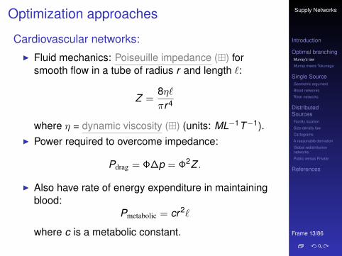
Cardiovascular networks:I Fluid mechanics: Poiseuille impedance () for

smooth flow in a tube of radius r and length `:

Z =8η`

πr4

where η = dynamic viscosity () (units: ML−1T−1).I Power required to overcome impedance:

Pdrag = Φ∆p = Φ2Z .

I Also have rate of energy expenditure in maintainingblood:

Pmetabolic = cr2`

where c is a metabolic constant.

http://en.wikipedia.org/wiki/Hagen-Poiseuille_equation

http://en.wikipedia.org/wiki/Dynamic_viscosity

Supply Networks

Introduction




Blood networks

River networks


Size-density law

Cartograms




References

Frame 14/86


Aside on Pdrag

I Work done = F · d = energy transferred by force FI Power = P = rate work is done = F · vI ∆p = Force per unit areaI Φ = Volume per unit time

= cross-sectional area · velocityI So Φ∆p = Force · velocity

Supply Networks

Introduction




Blood networks

River networks


Size-density law

Cartograms




References

Frame 15/86


Murray’s law:

I Total power (cost):

P = Pdrag + Pmetabolic = Φ2 8η`

πr4 + cr2`

I Observe power increases linearly with `

I But r ’s effect is nonlinear:I increasing r makes flow easier but increases

metabolic cost (as r2)I decreasing r decrease metabolic cost but impedance

goes up (as r−4)

Supply Networks

Introduction




Blood networks

River networks


Size-density law

Cartograms




References

Frame 16/86

Optimization

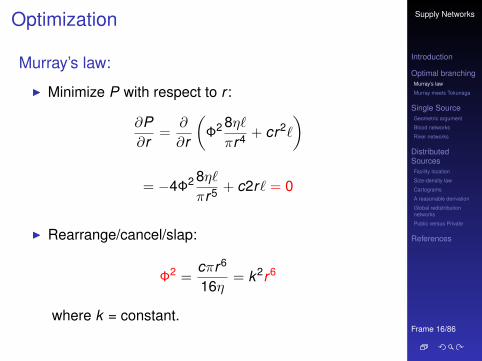
Murray’s law:

I Minimize P with respect to r :

∂P∂r

=∂

∂r

(Φ2 8η`

πr4 + cr2`

)

= −4Φ2 8η`

πr5 + c2r` = 0

I Rearrange/cancel/slap:

Φ2 =cπr6

16η= k2r6

where k = constant.

Supply Networks

Introduction




Blood networks

River networks


Size-density law

Cartograms




References

Frame 17/86

Optimization

Murray’s law:

I So we now have:Φ = kr3

I Flow rates at each branching have to add up (elseour organism is in serious trouble...):

Φ0 = Φ1 + Φ2

where again 0 refers to the main branch and 1 and 2refers to the offspring branches

I All of this means we have a groovy cube-law:

r30 = r3

1 + r32

Supply Networks

Introduction




Blood networks

River networks


Size-density law

Cartograms




References

Frame 19/86

Optimization

Murray meets Tokunaga:

I Φω = volume rate of flow into an order ω vesselsegment

I Tokunaga picture:

Φω = 2Φω−1 +ω−1∑k=1

TkΦω−k

I Using φω = kr3ω

r3ω = 2r3

ω−1 +ω−1∑k=1

Tk r3ω−k

I Find Horton ratio for vessel radius Rr = rω/rω−1...

Supply Networks

Introduction




Blood networks

River networks


Size-density law

Cartograms




References

Frame 20/86

Optimization


I Find R 3r satisfies same equation as Rn and Rv

(v is for volume):

R3r = Rn = Rv

I Is there more we could do here to constrain theHorton ratios and Tokunaga constants?

Supply Networks

Introduction




Blood networks

River networks


Size-density law

Cartograms




References

Frame 21/86

Optimization


I Isometry: Vω ∝ ` 3ω

I GivesR3

` = Rv = Rn

I We need one more constraint...I West et al (1997) [25] achieve similar results following

Horton’s laws.I So does Turcotte et al. (1998) [22] using Tokunaga

(sort of).

Supply Networks

Introduction




Blood networks

River networks


Size-density law

Cartograms




References

Frame 23/86

Geometric argument

I Consider one source supplying many sinks in avolume V d-dim. region in a D-dim. ambient space.

I Assume sinks are invariant.I Assume ρ = ρ(V ), i.e., ρ may vary with region’s

volume V .I See network as a bundle of virtual vessels:

I Q: how does the number of sustainable sinks Nsinksscale with volume V for the most efficient networkdesign?

I Or: what is the highest α for Nsinks ∝ V α?

Supply Networks

Introduction




Blood networks

River networks


Size-density law

Cartograms




References

Frame 24/86

Geometric argument

I Allometrically growing regions:

Ω Ω L’2

L 1 L’

2L

1

(V)(V’)

I Have d length scales which scale as

Li ∝ V γi where γ1 + γ2 + . . . + γd = 1.

I For isometric growth, γi = 1/d .I For allometric growth, we must have at least two of

the γi being different

Supply Networks

Introduction




Blood networks

River networks


Size-density law

Cartograms




References

Frame 25/86

Geometric argument

I Best and worst configurations (Banavar et al.)

a b

I Rather obviously:min Vnet ∝

∑distances from source to sinks.

Supply Networks

Introduction




Blood networks

River networks


Size-density law

Cartograms




References

Frame 26/86

Minimal network volume:

Real supply networks are close to optimal:J.S

tat.Mech.

(2006)P

01015Shape and efficiency in spatial distribution networks

(a) (b) (c) (d)

Figure 1. (a) Commuter rail network in the Boston area. The arrow marksthe assumed root of the network. (b) Star graph. (c) Minimum spanning tree.(d) The model of equation (3) applied to the same set of stations.

Table 1. Number of vertices n, route factor q, and total edge length for each ofthe networks described in the text, along with the equivalent results for the stargraphs and minimum spanning trees on the same vertices. (Note that the routefactor for the star graph is always 1 and so has been omitted from the table.)

Route factor Edge length (km)

Network n Actual MST Actual MST Star

Sewer system 23 922 1.59 2.93 498 421 102 998Gas (WA) 226 1.13 1.82 5578 4374 245 034Gas (IL) 490 1.48 2.42 6547 4009 59 595Rail 126 1.14 1.61 559 499 3 272

set of n − 1 edges joining them such that all vertices belong to a single component andthe sum of the lengths of the edges is minimized4.)

To make the comparison with the star graph, we consider the distance from each non-root vertex to the root, first along the edges of the network and second along a simpleEuclidean straight line, and calculate the mean ratio of these two distances over all suchvertices. Following [18], we refer to this quantity as the network’s route factor, and denoteit q:

q =1

n− 1

n−1∑

i=1

li0di0

, (1)

where li0 is the distance along the edges of the network from vertex i to the root (whichhas label 0), and di0 is the direct Euclidean distance. If there is more than one paththrough the network to the root, we take the shortest one. Thus, for example, q = 2would imply that on average the shortest path from a vertex to the root through thenetwork is twice as long as a direct straight-line connection. The smallest possible valueof the route factor is 1, which is achieved by the star graph.

The route factors for our four networks are shown in table 1. As we can see, thenetworks are remarkably efficient in this sense, with route factors quite close to 1. Values

4 If we are not restricted to the specified vertex set but are allowed to add vertices freely, then the optimal solutionis the Steiner tree; in practice we find that there is little difference between results for minimum spanning andSteiner trees in the present context.

doi:10.1088/1742-5468/2006/01/P01015 4

(2006) Gastner and Newman [8]: “Shape and efficiency inspatial distribution networks”

Supply Networks

Introduction




Blood networks

River networks


Size-density law

Cartograms




References

Frame 27/86

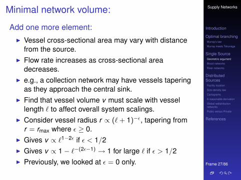
Minimal network volume:

Add one more element:I Vessel cross-sectional area may vary with distance

from the source.I Flow rate increases as cross-sectional area

decreases.I e.g., a collection network may have vessels tapering

as they approach the central sink.I Find that vessel volume v must scale with vessel

length ` to affect overall system scalings.I Consider vessel radius r ∝ (` + 1)−ε, tapering from

r = rmax where ε ≥ 0.I Gives v ∝ `1−2ε if ε < 1/2I Gives v ∝ 1− `−(2ε−1) → 1 for large ` if ε > 1/2I Previously, we looked at ε = 0 only.

Supply Networks

Introduction




Blood networks

River networks


Size-density law

Cartograms




References

Frame 28/86

Minimal network volume:For 0 ≤ ε < 1/2, approximate network volume by integralover region:

min Vnet ∝∫

Ωd,D(V )ρ ||~x ||1−2ε d~x

Insert question 1, assignment 3 ()

∝ ρV 1+γmax(1−2ε) where γmax = maxi

γi .

For ε > 1/2, find simply that

min Vnet ∝ ρV

I So if supply lines can taper fast enough and withoutlimit, minimum network volume can be madenegligible.

http://www.uvm.edu/~pdodds/teaching/courses/2010-01UVM-303/docs/2010-01UVM-303assignment3.pdf

Supply Networks

Introduction




Blood networks

River networks


Size-density law

Cartograms




References

Frame 29/86

Geometric argument

For 0 ≤ ε < 1/2:

I min Vnet ∝ ρV 1+γmax(1−2ε)

I If scaling is isometric, we have γmax = 1/d :

min Vnet/iso ∝ ρV 1+(1−2ε)/d

I If scaling is allometric, we have γmax = γallo > 1/d :and

min Vnet/allo ∝ ρV 1+(1−2ε)γallo

I Isometrically growing volumes require less networkvolume than allometrically growing volumes:

min Vnet/iso

min Vnet/allo→ 0 as V →∞

Supply Networks

Introduction




Blood networks

River networks


Size-density law

Cartograms




References

Frame 30/86

Geometric argument

For ε > 1/2:

I min Vnet ∝ ρVI Network volume scaling is now independent of

overall shape scaling.

Limits to scaling

I Can argue that ε must effectively be 0 for realnetworks over large enough scales.

I Limit to how fast material can move, and how smallmaterial packages can be.

I e.g., blood velocity and blood cell size.

Supply Networks

Introduction




Blood networks

River networks


Size-density law

Cartograms




References

Frame 32/86

Blood networks

I Velocity at capillaries and aorta approximatelyconstant across body size [24]: ε = 0.

I Material costly ⇒ expect lower optimal bound ofVnet ∝ ρV (d+1)/d to be followed closely.

I For cardiovascular networks, d = D = 3.I Blood volume scales linearly with blood volume [17],

Vnet ∝ V .I Sink density must ∴ decrease as volume increases:

ρ ∝ V−1/d .

I Density of suppliable sinks decreases with organismsize.

Supply Networks

Introduction




Blood networks

River networks


Size-density law

Cartograms




References

Frame 33/86

Blood networks

I Then P, the rate of overall energy use in Ω, can atmost scale with volume as

P ∝ ρV ∝ ρ M ∝ M (d−1)/d

I For d = 3 dimensional organisms, we have

P ∝ M 2/3

I Including other constraints may raise scalingexponent to a higher, less efficient value.

I Exciting bonus: Scaling obtained by the supplynetwork story and the surface-area law only matchfor isometrically growing shapes.Insert question 3, assignment 3 ()


Supply Networks

Introduction




Blood networks

River networks


Size-density law

Cartograms




References

Frame 34/86

Recap:

I The exponent α = 2/3 works for all birds andmammals up to 10–30 kg

I For mammals > 10–30 kg, maybe we have a newscaling regime

I Economos: limb length break in scaling around 20 kgI White and Seymour, 2005: unhappy with large

herbivore measurements. Find α ' 0.686± 0.014

Supply Networks

Introduction




Blood networks

River networks


Size-density law

Cartograms




References

Frame 36/86

River networks

I View river networks as collection networks.I Many sources and one sink.I ε?I Assume ρ is constant over time and ε = 0:

Vnet ∝ ρV (d+1)/d = constant× V 3/2

I Network volume grows faster than basin ‘volume’(really area).

I It’s all okay:Landscapes are d=2 surfaces living in D=3dimension.

I Streams can grow not just in width but in depth...I If ε > 0, Vnet will grow more slowly but 3/2 appears to

be confirmed from real data.

Supply Networks

Introduction




Blood networks

River networks


Size-density law

Cartograms




References

Frame 38/86

Many sources, many sinks

How do we distribute sources?I Focus on 2-d (results generalize to higher

dimensions)I Sources = hospitals, post offices, pubs, ...I Key problem: How do we cope with uneven

population densities?I Obvious: if density is uniform then sources are best

distributed uniformlyI Which lattice is optimal? The hexagonal lattice

Q1: How big should the hexagons be?I Q2: Given population density is uneven, what do we

do?I We’ll follow work by Stephan [18, 19], Gastner and

Newman (2006) [7], Um et al. [23] and work cited bythem.

Supply Networks

Introduction




Blood networks

River networks


Size-density law

Cartograms




References

Frame 39/86

Optimal source allocation

Solidifying the basic problem

I Given a region with some population distribution ρ,most likely uneven.

I Given resources to build and maintain N facilities.I Q: How do we locate these N facilities so as to

minimize the average distance between anindividual’s residence and the nearest facility?

Supply Networks

Introduction




Blood networks

River networks


Size-density law

Cartograms




References

Frame 40/86

Optimal source allocationThe value of s!r" is constrained by the requirement that

there be p facilities in total. Noting that s!r" is constant andequal to s!ri" within Voronoi cell Vi, we see that the integralof #s!r"$−1 over Vi is

%Vi

#s!r"$−1d2r = #s!ri"$−1%Vi

d2r = 1. !3"

Summing over all Vi, we can then express the constraint onthe number of facilities in the form

%A

#s!r"$−1d2r = p . !4"

Subject to this constraint, optimization of the mean dis-tance f above gives

!

!s!r"&g%A

"!r"#s!r"$1/2d2r − #'p − %A

#s!r"$−1d2r() = 0,

!5"

where # is a Lagrange multiplier. Performing the functionalderivatives and rearranging for s!r", we find s!r"= #2# / !g"!r""$2/3. The Lagrange multiplier can be evaluatedby substituting into Eq. !4", and we arrive at the result

D!r" =1

s!r"= p

#"!r"$2/3

% #"!r"$2/3d2r

, !6"

where we have introduced the notation D!r"= #s!r"$−1 for thedensity of the facilities.

Thus, if facilities are distributed optimally for the givenpopulation distribution, their density should increase withpopulation density but it should do so slower than linearly, asa power law with exponent 2

3 #29$. In addition to the argu-ment given here, which roughly follows Ref. #10$, this resulthas also been derived previously by a number of other meth-ods #5–9$, although all are approximate.

Equation !6" places most facilities in the densely popu-lated areas where most people live while still providing rea-sonable service to those in sparsely populated areas where astrictly population-proportional allocation might leave inhab-itants with little or nothing. Its derivation makes two ap-proximations: it assumes that the geometric factor g is thesame for all Voronoi cells and that s!r" is a continuous func-tion. Neither assumption is strictly true, but we expect themto be approximately valid if " varies little over the typicalsize of a Voronoi cell. As a test of these assumptions, wehave optimized numerically the distribution of p=5000 fa-cilities over the lower 48 states of the United States !Fig. 1"using population data from the most recent U.S. Census #11$,which counts the number of residents within more than 8million blocks across the study region. To create a continu-ous density function ", we convolved these data with a nor-malized Gaussian distribution of width 20 km #30$. The fa-cility locations were then determined by optimizing the fullp-median objective function !1" by simulated annealing #12$.

The relation D$"2/3 can be tested as follows. First, wedetermine the Voronoi cell around each facility. Then we

calculate D!r" as the inverse of the area of the correspondingcell and " as the number of people living in the cell dividedby its area. Figure 2 shows a scatter plot of the resulting dataon doubly logarithmic scales. If the anticipated 2

3-power re-lation holds, we expect the data to fall along a line of slope23 . And indeed a least-squares fit !solid line in the figure"yields a slope 0.66 with r2=0.94.

Some statistical concerns might be raised about thismethod. First, we used the Voronoi cell area to calculate bothD and ", so the measurements of x and y values in the plotare not independent, and one might argue that a positiveslope could thus be a result of artificial correlations betweenthe values rather than a real result #13$. Second, it is knownthat estimating the exponent of a power law such as Eq. !6"from a log-log plot can introduce systematic biases #14,15$.In the next section, we introduce an entirely different test ofEq. !6" that, in addition to being of interest in its own right,suffers from neither of these problems.

III. DENSITY-EQUALIZING PROJECTIONS

If we neglect finite-size effects, it is straightforward todemonstrate that optimally located facilities in a uniformly

FIG. 1. !Color online" Facility locations determined by simu-lated annealing and the corresponding Voronoi tessellation for p=5000 facilities located in the lower 48 United States, based onpopulation data from the U.S. Census for the year 2000.

FIG. 2. !Color online" Facility density D from Fig. 1 vs popu-lation density " on a log-log plot. A least-squares linear fit to thedata gives a slope of 0.66 !solid line, r2=0.94".

MICHAEL T. GASTNER AND M. E. J. NEWMAN PHYSICAL REVIEW E 74, 016117 !2006"

016117-2

From Gastner and Newman (2006) [7]

I Approximately optimal location of 5000 facilities.

I Based on 2000 Census data.

I Simulated annealing + Voronoi tessellation.

Supply Networks

Introduction




Blood networks

River networks


Size-density law

Cartograms




References

Frame 41/86


The value of s!r" is constrained by the requirement thatthere be p facilities in total. Noting that s!r" is constant andequal to s!ri" within Voronoi cell Vi, we see that the integralof #s!r"$−1 over Vi is

%Vi

#s!r"$−1d2r = #s!ri"$−1%Vi

d2r = 1. !3"

Summing over all Vi, we can then express the constraint onthe number of facilities in the form

%A

#s!r"$−1d2r = p . !4"

Subject to this constraint, optimization of the mean dis-tance f above gives

!

!s!r"&g%A

"!r"#s!r"$1/2d2r − #'p − %A

#s!r"$−1d2r() = 0,

!5"

where # is a Lagrange multiplier. Performing the functionalderivatives and rearranging for s!r", we find s!r"= #2# / !g"!r""$2/3. The Lagrange multiplier can be evaluatedby substituting into Eq. !4", and we arrive at the result

D!r" =1

s!r"= p

#"!r"$2/3

% #"!r"$2/3d2r

, !6"

where we have introduced the notation D!r"= #s!r"$−1 for thedensity of the facilities.

Thus, if facilities are distributed optimally for the givenpopulation distribution, their density should increase withpopulation density but it should do so slower than linearly, asa power law with exponent 2

3 #29$. In addition to the argu-ment given here, which roughly follows Ref. #10$, this resulthas also been derived previously by a number of other meth-ods #5–9$, although all are approximate.

Equation !6" places most facilities in the densely popu-lated areas where most people live while still providing rea-sonable service to those in sparsely populated areas where astrictly population-proportional allocation might leave inhab-itants with little or nothing. Its derivation makes two ap-proximations: it assumes that the geometric factor g is thesame for all Voronoi cells and that s!r" is a continuous func-tion. Neither assumption is strictly true, but we expect themto be approximately valid if " varies little over the typicalsize of a Voronoi cell. As a test of these assumptions, wehave optimized numerically the distribution of p=5000 fa-cilities over the lower 48 states of the United States !Fig. 1"using population data from the most recent U.S. Census #11$,which counts the number of residents within more than 8million blocks across the study region. To create a continu-ous density function ", we convolved these data with a nor-malized Gaussian distribution of width 20 km #30$. The fa-cility locations were then determined by optimizing the fullp-median objective function !1" by simulated annealing #12$.

The relation D$"2/3 can be tested as follows. First, wedetermine the Voronoi cell around each facility. Then we

calculate D!r" as the inverse of the area of the correspondingcell and " as the number of people living in the cell dividedby its area. Figure 2 shows a scatter plot of the resulting dataon doubly logarithmic scales. If the anticipated 2

3-power re-lation holds, we expect the data to fall along a line of slope23 . And indeed a least-squares fit !solid line in the figure"yields a slope 0.66 with r2=0.94.

Some statistical concerns might be raised about thismethod. First, we used the Voronoi cell area to calculate bothD and ", so the measurements of x and y values in the plotare not independent, and one might argue that a positiveslope could thus be a result of artificial correlations betweenthe values rather than a real result #13$. Second, it is knownthat estimating the exponent of a power law such as Eq. !6"from a log-log plot can introduce systematic biases #14,15$.In the next section, we introduce an entirely different test ofEq. !6" that, in addition to being of interest in its own right,suffers from neither of these problems.

III. DENSITY-EQUALIZING PROJECTIONS

If we neglect finite-size effects, it is straightforward todemonstrate that optimally located facilities in a uniformly

FIG. 1. !Color online" Facility locations determined by simu-lated annealing and the corresponding Voronoi tessellation for p=5000 facilities located in the lower 48 United States, based onpopulation data from the U.S. Census for the year 2000.

FIG. 2. !Color online" Facility density D from Fig. 1 vs popu-lation density " on a log-log plot. A least-squares linear fit to thedata gives a slope of 0.66 !solid line, r2=0.94".


016117-2


I Optimal facility density D vs. population density ρ.I Fit is D ∝ ρ0.66 with r2 = 0.94.I Looking good for a 2/3 power...

Supply Networks

Introduction




Blood networks

River networks


Size-density law

Cartograms




References

Frame 43/86


Size-density law:

I

D ∝ ρ2/3

I Why?I Again: Different story to branching networks where

there was either one source or one sink.I Now sources & sinks are distributed throughout

region...

Supply Networks

Introduction




Blood networks

River networks


Size-density law

Cartograms




References

Frame 44/86


I We first examine Stephan’s treatment (1977) [18, 19]

I “Territorial Division: The Least-Time ConstraintBehind the Formation of Subnational Boundaries”(Science, 1977)

I Zipf-like approach: invokes principle of minimal effort.I Also known as the Homer principle.

Supply Networks

Introduction




Blood networks

River networks


Size-density law

Cartograms




References

Frame 45/86


I Consider a region of area A and population P with asingle functional center that everyone needs toaccess every day.

I Build up a general cost function based on timeexpended to access and maintain center.

I Write average travel distance to center as d andassume average speed of travel is v .

I Assume isometry: average travel distance d will beon the length scale of the region which is ∼ A1/2

I Average time expended per person in accessingfacility is therefore

d/v = cA1/2/v

where c is an unimportant shape factor.

Supply Networks

Introduction




Blood networks

River networks


Size-density law

Cartograms




References

Frame 46/86


I Next assume facility requires regular maintenance(person-hours per day)

I Call this quantity τ

I If burden of mainenance is shared then average costper person is τ/P where P = population.

I Replace P by ρA where ρ is density.I Total average time cost per person:

T = d/v + τ/(ρA) = gA1/2/v + τ/(ρA).

I Now Minimize with respect to A...

Supply Networks

Introduction




Blood networks

River networks


Size-density law

Cartograms




References

Frame 47/86

Optimal source allocationI Differentiating...

∂T∂A

=∂

∂A

(cA1/2/v + τ/(ρA)

)=

c2vA1/2 −

τ

ρA2 = 0

I Rearrange:

A =

(2vτ

cρ

)2/3

∝ ρ−2/3

I # facilities per unit area ∝

A−1 ∝ ρ2/3

I Groovy...

Supply Networks

Introduction




Blood networks

River networks


Size-density law

Cartograms




References

Frame 48/86


An issue:I Maintenance (τ ) is assumed to be independent of

population and area (P and A)

Supply Networks

Introduction




Blood networks

River networks


Size-density law

Cartograms




References

Frame 49/86


Stephan’s online book“The Division of Territory in Society” is here ().

http://www.ac.wwu.edu/~stephan/Book/contents.html

Supply Networks

Introduction




Blood networks

River networks


Size-density law

Cartograms




References

Frame 51/86

Cartograms

Standard world map:

Supply Networks

Introduction




Blood networks

River networks


Size-density law

Cartograms




References

Frame 52/86

Cartograms

Cartogram of countries ‘rescaled’ by population:

Supply Networks

Introduction




Blood networks

River networks


Size-density law

Cartograms




References

Frame 53/86

Cartograms

Diffusion-based cartograms:

I Idea of cartograms is to distort areas to moreaccurately represent some local density ρ (e.g.population).

I Many methods put forward—typically involve somekind of physical analogy to spreading or repulsion.

I Algorithm due to Gastner and Newman (2004) [6] isbased on standard diffusion:

∇2ρ− ∂ρ

∂t= 0.

I Allow density to diffuse and trace the movement ofindividual elements and boundaries.

I Diffusion is constrained by boundary condition ofsurrounding area having density ρ.

Supply Networks

Introduction




Blood networks

River networks


Size-density law

Cartograms




References

Frame 54/86

Cartograms

Child mortality:

Supply Networks

Introduction




Blood networks

River networks


Size-density law

Cartograms




References

Frame 55/86

Cartograms

Energy consumption:

Supply Networks

Introduction




Blood networks

River networks


Size-density law

Cartograms




References

Frame 56/86

Cartograms

Gross domestic product:

Supply Networks

Introduction




Blood networks

River networks


Size-density law

Cartograms




References

Frame 57/86

Cartograms

Greenhouse gas emissions:

Supply Networks

Introduction




Blood networks

River networks


Size-density law

Cartograms




References

Frame 58/86

Cartograms

Spending on healthcare:

Supply Networks

Introduction




Blood networks

River networks


Size-density law

Cartograms




References

Frame 59/86

Cartograms

People living with HIV:

Supply Networks

Introduction




Blood networks

River networks


Size-density law

Cartograms




References

Frame 60/86

Cartograms

I The preceding sampling of Gastner & Newman’scartograms lives here ().

I A larger collection can be found atworldmapper.org ().

http://www-personal.umich.edu/~mejn/cartograms/

http://www.worldmapper.org/

Supply Networks

Introduction




Blood networks

River networks


Size-density law

Cartograms




References

Frame 61/86

Size-density law

populated space lie on the vertices of a regular triangularlattice !16". It has been conjectured that for a non uniformpopulation there is a general class of map projections thatwill transform the pattern of facilities to a similarly regularstructure !17". The obvious candidate projections are popu-lation density equalizing maps or cartograms, i.e., maps inwhich the sizes of geographic regions are proportional to thepopulations of those regions !18–21". Densely populated re-gions appear larger on a cartogram than on an equal-areamap such as Fig. 1, and the opposite is true for sparselypopulated regions. Since most facilities are located where thepopulation density is high, a cartogram projection will effec-tively reduce the facility density in populated areas and in-crease it where the population density is low. Therefore, onemight expect that a cartogram leads to a more uniform facil-ity density than that shown in Fig. 1. And indeed some au-thors have used population density equalizing projections asthe basis for facility location methods !22,23".

In Fig. 3#a$, we show the facilities of Fig. 1 on a popula-tion density equalizing cartogram created using thediffusion-based technique of !24". Although the populationdensity is now equal everywhere, the facility density is ob-viously far from uniform. A comparison between Figs. 1 and3#a$ reveals that we have overshot the mark since the facili-ties are now concentrated in areas where there are few inactual space.

Equation #6$ makes clear what is wrong with this ap-proach. Since D grows slower than linearly with !, a projec-tion that equalizes ! will necessarily overcorrect the densityof facilities. On the other hand, based on our earlier result,we would expect a projection equalizing !2/3 instead of ! tospread out the facilities approximately uniformly. Hence, oneway to determine the actual exponent for the density of fa-cilities is to create cartograms that equalize !x, x"0, andfind the value of x that minimizes the variation of theVoronoi cell sizes on the cartogram. This approach does notsuffer from the shortcomings of our previous method basedon the doubly logarithmic plot in Fig. 2, since we neither usethe Voronoi cells to calculate the population density nor takelogarithms. One might argue that the Voronoi cells on thecartogram are not equal to the projections of the Voronoicells in actual space, which is true—the cells generally willnot even remain polygons under the cartogram transforma-tion. The difference, however, is small if the density does notvary much between neighboring facilities.

In Fig. 4, we show the measured coefficient of variation#i.e., the ratio of the standard deviation to the mean$ forVoronoi cell sizes on !x cartograms as a function of the ex-

ponent x #solid curve$. As the figure shows, the minimum isindeed attained at or close to the predicted value of x= 2

3 .Figure 3#b$ shows the corresponding cartogram for this ex-ponent. This projection finds a considerably better compro-mise between regions of high and low population densitythan either Fig. 1 or Fig. 3#a$.

For comparison, we have also made the same measure-ment for 5000 points distributed randomly in proportion topopulation. Since the density of these points is by definitionequal to !, we expect the minimum standard deviation of thecell areas to occur on a cartogram with x=1. Our numericalresults for this case #dashed curve in Fig. 4$ agree well withthis prediction. Comparing the solid and the dashed curves inthe plot, we see that not only the positions of the minimadiffer, but also the minimal values themselves. The lowerstandard deviation for the p-median distribution indicatesthat optimally located facilities are not randomly distributedwith a density #!2/3. Instead, the optimally located facilitiesoccupy space in a relatively regular fashion reminiscent ofthe triangular lattice of the uniform population case !16,25".We can confirm this observation by measuring the interiorangles formed by the edges of the Voronoi cells. The Voronoicells of a triangular lattice are regular hexagons and hence allthe interior angles are 120°. Figure 5 shows a histogram ofthe angles for the cells in the equal-area projection of Fig. 1.Since the population is nonuniform, the cells are not exactlyregular hexagons, but, as Fig. 5 shows, the angles are none-

FIG. 3. #Color online$ Near-optimal facility location on #a$ acartogram equalizing the popula-tion density ! and #b$ a cartogramequalizing !2/3.

FIG. 4. #Color online$ The coefficient of variation #i.e., the ratioof the standard deviation to the mean$ for Voronoi cell areas as theyappear on a cartogram, against the exponent x of the underlyingdensity !x for a p-median #solid curve$ and a random population-proportional distribution #dashed curve$. Inset: An expanded viewof the minimum for the p-median distribution.

OPTIMAL DESIGN OF SPATIAL DISTRIBUTION NETWORKS PHYSICAL REVIEW E 74, 016117 #2006$

016117-3

I Left: population density-equalized cartogram.I Right: (population density)2/3-equalized cartogram.I Facility density is uniform for ρ2/3 cartogram.


Supply Networks

Introduction




Blood networks

River networks


Size-density law

Cartograms




References

Frame 62/86

Size-density law

theless narrowly distributed around 120°—more so than forthe cells of the random distribution.

IV. OPTIMAL NETWORKS OF FACILITIES

In many cases of practical interest, finding the optimallocation of facilities is only half the problem. Often facilitiesare interconnected to form networks, such as airports con-nected by flights or warehouses connected by truck deliver-ies. In these cases, one would also like to find the best way toconnect the facilities so as to optimize the performance of thesystem as a whole.

Consider then a situation in which our facilities form thenodes or vertices of a network and connections betweenthem form the edges. The efficiency of this network, as wewill consider it here, depends on two factors. On the onehand, the smaller the sum of the lengths of all edges, thecheaper the network is to construct and maintain. On theother hand, the shorter the distances through the networkbetween vertices, the faster the network can perform its in-tended function !e.g., transportation of passengers betweennodes or distribution of mail or cargo". These two objectivesgenerally oppose each other: a network with few and shortconnections will not provide many direct links between dis-tant points, and paths through the network will tend to becircuitous, while a network with a large number of directlinks is usually expensive to build and operate. The optimalsolution lies somewhere between these extremes.

Let us define lij to be the shortest geographic distancebetween two vertices i and j measured along the edges in thenetwork. If there is no path between i and j, we formally setlij =!. Introducing the adjacency matrix A with elementsAij =1 if there is an edge between i and j and Aij =0 other-wise, we can write the total length of all edges as

T = #i"j

Aijlij . !7"

We assume this quantity to be proportional to the cost ofmaintaining the network. Clearly this assumption is only ap-proximately correct; networked systems in the real worldwill have many factors affecting their maintenance costs thatare not accounted for here. It is, however, the obvious firstassumption to make and, as we will see, can provide us withgood insight about network structure.

The typical cost of shipping a commodity or travelingthrough the network depends on the distances lij as well asthe amount of traffic wij !e.g., weight of cargo, number ofpassengers, etc." that flows between vertices i and j $26%. Ina spirit similar to our assumption about maintenance costs,we assume that the total travel cost is proportional to

Z = #i"j

wijlij . !8"

We assume that wij is proportional to the product of popula-tions in the Voronoi cells Vi and Vj around i and j, so that

wij = &Vi

#!r"d2r&Vj

#!r!"d2r! !9"

in appropriate units. And the total cost of running the net-work is proportional to the sum T+$Z with $%0 a constantthat measures the relative importance of the two terms. Thenthe optimal network is the one minimizing this sum $27,28%.

Using again the contiguous 48 states of the United Statesas an example, we have first determined the optimal place-ment of p=200 facilities, which we then try to connect to-gether optimally. The number of edges in the network de-pends on the parameter $. If $→0, the cost of travel $Zvanishes and the optimal network is the one that simplyminimizes the total length of edges. That is, it is the mini-mum spanning tree, with exactly p−1 edges between the pvertices. Conversely, if $→!, then Z dominates the optimi-zation, regardless of the cost T of maintaining the network,so that the optimum is a fully connected network or cliquewith all 1

2 p!p−1" possible edges present. For intermediatevalues of $, finding the optimal network is a nontrivial com-binatorial optimization problem. The number of edges in-creases with $, but it is difficult to determine the exact set ofedges optimizing the cost. Nevertheless, we can derive good,though usually not perfect, solutions using again the methodof simulated annealing $31%.

There is, however, another complicating factor. In Eq. !8",we assumed that travel costs are proportional to geometricdistances between vertices, which is a plausible startingpoint. In a road network, for example, the quickest andcheapest route is usually not very different from the shortestroute measured in kilometers. But in other networks, travelcosts can also depend on the number of legs in a journey. Inan airline network, for instance, passengers often spend a lotof time waiting for connecting flights, so that they care bothabout the total distance they travel and the number of stop-overs they have to make. Similarly, the total time requiredfor an Internet packet to reach its destination depends on twofactors, the propagation delay proportional to the physicaldistance between vertices !computers and routers" and thestore and forward delays introduced by the routers, whichgrow with the number of intermediate vertices.

To account for such situations, we generalize our defini-tion of the length of an edge and assign to each edge aneffective length

FIG. 5. !Color online" The distribution of angles in the Voronoidiagram for a p-median and a random population-proportional dis-tribution of facilities.


016117-4


I Cartogram’s Voronoi cells are somewhat hexagonal.

Supply Networks

Introduction




Blood networks

River networks


Size-density law

Cartograms




References

Frame 64/86

Size-density law

Deriving the optimal source distribution:

I Basic idea: Minimize the average distance from arandom individual to the nearest facility. [7]

I Assume given a fixed population density ρ defined ona spatial region Ω.

I Formally, we want to find the locations of n sources~x1, . . . , ~xn that minimizes the cost function

F (~x1, . . . , ~xn) =

∫Ω

ρ(~x) mini||~x − ~xi ||d~x .

I Also known as the p-median problem.I Not easy... in fact this one is an NP-hard problem. [7]

I Approximate solution originally due toGusein-Zade [9].

Supply Networks

Introduction




Blood networks

River networks


Size-density law

Cartograms




References

Frame 65/86

Size-density law

Approximations:

I For a given set of source placements ~x1, . . . , ~xn,the region Ω is divided up into Voronoi cells (), oneper source.

I Define A(~x) as the area of the Voronoi cell containing~x .

I As per Stephan’s calculation, estimate typicaldistance from ~x to the nearest source (say i) as

ciA(~x)1/2

where ci is a shape factor for the i th Voronoi cell.I Approximate ci as a constant c.

http://en.wikipedia.org/wiki/Voronoi_diagram

Supply Networks

Introduction




Blood networks

River networks


Size-density law

Cartograms




References

Frame 66/86

Size-density law

Carrying on:

I The cost function is now

F = c∫

Ωρ(~x)A(~x)1/2d~x .

I We also have that the constraint that Voronoi cellsdivide up the overall area of Ω:

∑ni=1 A(~xi) = AΩ.

I Sneakily turn this into an integral constraint:∫Ω

d~xA(~x)

= n.

I Within each cell, A(~x) is constant.I So... integral over each of the n cells equals 1.

Supply Networks

Introduction




Blood networks

River networks


Size-density law

Cartograms




References

Frame 67/86

Size-density lawNow a Lagrange multiplier story:

I By varying ~x1, ..., ~xn, minimize

G(A) = c∫

Ωρ(~x)A(~x)1/2d~x −λ

(n −

∫Ω

[A(~x)

]−1 d~x)

I Next compute δG/δA, the functional derivative () ofthe functional G(A).

I This gives∫Ω

[c2ρ(~x)A(~x)−1/2 − λ

[A(~x)

]−2]

d~x = 0.

I Setting the integrand to be zilch, we have:

ρ(~x) = 2λc−1A(~x)−3/2.

http://en.wikipedia.org/wiki/Functional_derivative

Supply Networks

Introduction




Blood networks

River networks


Size-density law

Cartograms




References

Frame 68/86

Size-density lawNow a Lagrange multiplier story:

I Rearranging, we have

A(~x) = (2λc−1)2/3ρ−2/3.

I Finally, we indentify 1/A(~x) as D(~x), anapproximation of the local source density.

I Substituting D = 1/A, we have

D(~x) =( c

2λρ)2/3

.

I Normalizing (or solving for λ):

D(~x) = n[ρ(~x)]2/3∫

Ω[ρ(~x)]2/3d~x∝ [ρ(~x)]2/3.

Supply Networks

Introduction




Blood networks

River networks


Size-density law

Cartograms




References

Frame 70/86

Global redistribution networks

One more thing:

I How do we supply these facilities?I How do we best redistribute mail? People?I How do we get beer to the pubs?I Gaster and Newman model: cost is a function of

basic maintenance and travel time:

Cmaint + γCtravel.

I Travel time is more complicated: Take ‘distance’between nodes to be a composite of shortest pathdistance `ij and number of legs to journey:

(1− δ)`ij + δ(#hops).

I When δ = 1, only number of hops matters.

Supply Networks

Introduction




Blood networks

River networks


Size-density law

Cartograms




References

Frame 71/86

Global redistribution networks

li j = !1 − !"lij + ! !10"

with 0"!"1. The parameter ! determines the user’s pref-erence for measuring distance in terms of kilometers or legs.Now we define the effective distance between two !not nec-essarily adjacent" vertices to be the sum of the effectivelengths of all edges along a path between them, minimizedover all paths. The travel cost is then proportional to the sumof all effective path lengths

Z = #i#j

wijlij , !11"

and the optimal network for given $ and ! is again the onethat minimizes the total cost T+$Z. Since the second term inEq. !10" is dimensionless, we normalize the length appearingin the first term by setting the average “crow flies” distancebetween a vertex and its nearest neighbor equal to 1.

What is a realistic value for $? We can make an order ofmagnitude estimate as follows. The sum in Eq. !7" has mnonzero terms, where m is the number of edges in the net-work. Most real networks are sparse, with m=O!p". Further-more, edges are of typical length 1 in our length scale, sothat T=O!p", with p$200 in the examples studied here. Thesum in Eq. !11", on the other hand, contains 1

2 p!p−1"=O!p2" nonzero terms. If P is the total population, theweights wij have typical value !P / p"2. Thus Z=O!P2"$1017 for the U.S. with a current population of P$2.8%108. Assuming that our investments in maintenance andtravel costs are of the same order of magnitude and settingT%$Z then leads to an estimate for $ of order 10−15or 10−14.

In Fig. 6, we show the results for $=10−14. When !=0,passengers !or cargo shippers" care only about total kilome-ters traveled and the optimal network strongly resembles anetwork of roads, such as the U.S. interstate network. As !increases, the number of legs in a journey starts playing amore important role and the approximate symmetry betweenthe vertices is broken as the network begins to form hubs.

Around !=0.5, we see networks emerging that constitute acompromise between the convenience of direct local connec-tions and the efficiency of hubs, while by !=0.8 the networkis dominated by a few large hubs in Philadelphia, Columbus,Chicago, Kansas City, and Atlanta that handle the bulk of thetraffic. On the highly populated California coast, two smallerhubs around San Francisco and Los Angeles are visible. Inthe extreme case !=1, where the user cares only about num-ber of legs and not about distance at all, the network is domi-nated by a single central hub in Cincinnati, with a fewsmaller local hubs in other locations such as Los Angeles.

V. CONCLUSIONS

We have studied the problem of optimal facility location,also called the p-median problem, which consists of choos-ing positions for p facilities in geographic space such that themean distance between a member of the population and thenearest facility is minimized. Analytic arguments indicatethat the optimal density of facilities should be proportional tothe population density to the two-thirds power. We have con-firmed this relation by solving the p-median problem numeri-cally and projecting the facility locations on density-equalizing maps. We have also considered the design ofoptimal networks to connect our facilities together. Givenoptimally located facilities, we have searched numericallyfor the network configuration that minimizes the sum ofmaintenance and travel costs. A simple two-parameter modelallows us to take different user preferences into account. Themodel gives us intuition about a number of situations ofpractical interest, such as the design of transportation net-works, parcel delivery services, and the Internet backbone.

ACKNOWLEDGMENTS

The authors thank the staff of the University of Michi-gan’s Numeric and Spatial Data Services for their help. Thiswork was funded in part by the National Science Foundationunder Grant No. DMS–0405348 and by the James S. Mc-Donnell Foundation.

FIG. 6. !Color online" Optimalnetworks for the population distri-bution of the United States withp=200 vertices and $=10−14 fordifferent values of !.

OPTIMAL DESIGN OF SPATIAL DISTRIBUTION NETWORKS PHYSICAL REVIEW E 74, 016117 !2006"

016117-5


Supply Networks

Introduction




Blood networks

River networks


Size-density law

Cartograms




References

Frame 73/86

Public versus private facilities

Beyond minimizing distances:

I “Scaling laws between population and facilitydensities” by Um et al., Proc. Natl. Acad. Sci.,2009. [23]

I Um et al. find empirically and argue theoretically thatthe connection between facility and populationdensity

D ∝ ρα

does not universally hold with α = 2/3.I Two idealized limiting classes:

1. For-profit, commercial facilities: α = 1;2. Pro-social, public facilities: α = 2/3.

I Um et al. investigate facility locations in the UnitedStates and South Korea.

Supply Networks

Introduction




Blood networks

River networks


Size-density law

Cartograms




References

Frame 74/86

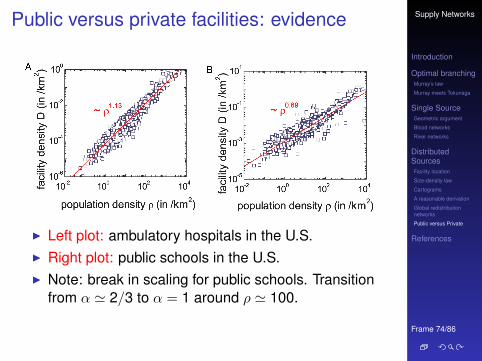
Public versus private facilities: evidence

APP

LIED

PHYS

ICA

LSC

IEN

CES

SOCI

AL

SCIE

NCE

S

Fig. 1. Scatter plots of population and facility density obtained from empir-ical data. (A) Facility density D versus population density ρ for ambulatoryhospitals in the US. (B) D versus ρ for the public schools in the US. For ambula-tory hospital the exponent is 1.13 close to 1, which shows clearly a differentdistribution from the exponent 0.69 for public schools. The public schoolshows roughly 2 regimes of different exponents around ρ ∼ 100/km2. Theregion above 100/km2 of population density shows the exponent as ≈1, andthe region below 100/km2 shows 2/3. The population density 100/km2 corre-sponds to the cross-over point of the facility density 0.03/km2, which meansthat 1 school covers about 33 km2. If we assume the geometry is nearly acircle, the radius of the attending distance is ≈3 km. For attending distances<3 km, public school distribution also shows similar behaviors to those of theprivate schools.

Voronoi cell. However, due to the resolution limitation of the facil-ity positions, we measure the scaling relation by using the numberof people and facilities of each county instead as a coarse-grainedscheme (see the Materials and Methods for details). From an analy-sis of the data, it was found in both the US and SK that althoughthe commercial facilities tend to have an exponent α ≈ 1, the pub-lic facilities commonly have an exponent α ≈ 2/3. For commercialfacilities such as ambulatory hospitals, the exponent α was foundto be 1.13 (top), for public facilities such as schools, the exponentwas 0.69 (bottom), as shown in Fig. 1. The other results for variousfacilities in US and SK are summarized in Table 1.

Interestingly, as a border of exponent 0.8 in Table 1, each facilityis clearly classified into 2 categories, commercial and public. In theUS data, ‘ambulatory hospital,’ ‘beauty care,’ ‘laundry,’ ‘automo-tive repair,’ ‘private school,’ ‘restaurant,’ ‘accommodation,’ ‘bank,’and ‘gas station’ are categorized as commercial facilities moreor less, whereas ‘death care,’ ‘fire station,’ ‘police station,’ and‘public school’ are categorized as public facilities, which provide

social welfare services. Even though the 2 countries have verydifferent physical, economic, sociocultural, and political environ-ments, (such as different topography, urban formations, popula-tion densities, standards of living, and cultures), similar facilities,like the ambulatory hospital in the US and the primary clinic inSK, have similar exponents.

It should be noted, however, that due to the differences in theeducational systems in the US and SK, the result-related schoolsystem is somewhat different. Because the US has a K-12 educa-tional system both in the public and private sectors, the table showsthe exponent 0.95 for private schools and 0.69 for public schools. InSK, even though there is a distinction between public and privateschools, this distinction is deceptive, as most students are allocatedto public and private schools by the ministry of education withoutany preference between private and public school. Therefore, theexponent of primary and secondary schools in SK is the same, 0.77,close to the public facilities and proving no distinction between pri-vate and public schools in SK. However, ‘university/college,’ whichis a more profit-driven type of school in SK shows α ∼ 0.93, closeto the commercial facility.

As a result, the social facilities, such as police and fire stationsand government offices, have respectively low exponents closeto 2/3. One of major differences between public and commer-cial facilities is probably the distance between these facilities andtheir clients. This is especially the case with respect to social facili-ties. For example, fire stations need to be located close to people’sresidences, so that fire fighters can serve quickly if needed, andthe same applies to police stations. For a school student, the com-mute distance is also important. As an extreme case, public health

Table 1. Summary of the exponents

US facility α (SE) R2

Ambulatory hospital 1.13(1) 0.93Beauty care 1.08(1) 0.86Laundry 1.05(1) 0.90Automotive repair 0.99(1) 0.92Private school 0.95(1) 0.82Restaurant 0.93(1) 0.89Accommodation 0.89(1) 0.70Bank 0.88(1) 0.89Gas station 0.86(1) 0.94

Death care 0.79(1) 0.80* Fire station 0.78(3) 0.93* Police station 0.71(6) 0.75Public school 0.69(1) 0.87

SK facility α (SE) R2

Bank 1.18(2) 0.96Parking place 1.13(2) 0.91* Primary clinic 1.09(2) 1.00* Hospital 0.96(5) 0.97* University/college 0.93(9) 0.89Market place 0.87(2) 0.90

* Secondary school 0.77(3) 0.98* Primary school 0.77(3) 0.97Social welfare org. 0.75(2) 0.84* Police station 0.71(5) 0.94Government office 0.70(1) 0.93* Fire station 0.60(4) 0.93* Public health center 0.09(5) 0.19

Summary of the values of α in D ∼ ρα for various facilities in the US andSK. The coefficient of determination R2 is obtained through the least-squaresanalysis. The value for each facility type is obtained from information in thecounty level, except for the asterisk(*)-marked values, which are from thestate level (US) and the province level (SK). The numbers in parentheses arethe standard errors in the last digits.

Um et al. PNAS August 25, 2009 vol. 106 no. 34 14237

APP

LIED

PHYS

ICA

LSC

IEN

CES

SOCI

AL

SCIE

NCE

S
















I Left plot: ambulatory hospitals in the U.S.I Right plot: public schools in the U.S.I Note: break in scaling for public schools. Transition

from α ' 2/3 to α = 1 around ρ ' 100.

Supply Networks

Introduction




Blood networks

River networks


Size-density law

Cartograms




References

Frame 75/86


APP

LIED

PHYS

ICA

LSC

IEN

CES

SOCI

AL

SCIE

NCE

S
















APP

LIED

PHYS

ICA

LSC

IEN

CES

SOCI

AL

SCIE

NCE

S
















Rough transitionbetween publicand private atα ' 0.8.

Note: * indicatesanalysis is atstate/provincelevel; otherwisecounty level.

Supply Networks

Introduction




Blood networks

River networks


Size-density law

Cartograms




References

Frame 76/86


Fig. 2. Distribution of public and private facilities. Density plot for ambulatory hospitals (A) and public schools (B) in the US. Voronoi cell diagram from modelsimulation for commercial (C) and public facilities (D). Note that the spatial distribution in B and D for public facilities is more uniform than that in A and C forcommercial facilities.

centers in SK show the exponent 0.09. Public health centers are dis-tributed almost evenly independent of population density becausetheir role is to support the medical service to persons who live ina very backward part of the country with no hospital. However,a commercial facility does not care much about how long theirclients need to travel, only about how many clients come.

Microdynamics Model for Economic ActivityIn our model, we consider the microdynamics for each facilityof 2 different types, namely commercial and public. Let us con-sider that there exist several identical facilities on a given area Awhere populations are allocated unevenly. We assume that peo-ple visit their nearest facility following the first law of geography:“Everything is related to everything else, but near things are morerelated than distant things” (12). For convenience, we introducethe Voronoi cell Vi as the set of points closer to the ith facilitythan to any other facilities within the area A (11). Therefore, thenumber of visitors to the ith facility is the number of people livingin the ith Voronoi cell Vi. We define the area of Vi as si and thepopulation living in Vi as ni.

First, for the commercial facilities, the profit of the ith facilitywould be proportional to ni, the number of potential customers,as we discussed above. We assume that every facility has a similarmaintenance expense ignoring the spatial inequality; therefore, aowner of the facility having lower ni is better off moving his/herfacility to the location near the facility that gets the higher profit.It is natural procedure following the efficient market hypothesis,which is well known in economics. For example, when facilities areevenly distributed, the facilities in a highly populated area shouldmake higher profits because ni is proportional to the populationdensity. Consequently, we expect that the owners of facilities in aplace with a low population density will want to move their facili-ties to a location with a higher population density. After relocatingthese facilities, more facilities will exist in the highly populatedplaces than the sparsely populated ones. It is notable that the relo-cation of facilities in this way should result in almost the same profitfor every facility, i.e., ni ≈ Np/Nf for all facilities, where Np is thetotal population and Nf is the number of facilities. If the positionsof facilities are optimized by consecutive relocations according to

ni, the number of visitor ni becomes almost the same with eachother, and facilities no longer have to change their location. Byusing the Voronoi cell and its area si, we obtain the expressionsof the population density at certain position r, ρ(r) = n(r)/s(r)in continuous form and the facility density D(r) = 1/s(r), wheren(r) = ni and s(r) = si if r ∈ Vi. At the steady state, n(r) ≈ Np/Nfleads to

D(r) ≈ Nf

Npρ(r). [1]

From Eq. 1, we reach the conclusion that the exponent α =1 for the commercial facilities is consistent with the empiricaldata.

Now, we expand the above argument to the public facility.For the positioning of public facilities, however, the governmentshould consider not the profit but a social opportunity cost causedby the distance between visitors and facilities. The summationof travel distance (cost) ci from each visitor to the ith facility iswritten as

ci =∑

k∈P(Vi)

|rik| = ni〈ri〉, [2]

where P(Vi) is the set of a population within Vi and |rik| representsthe distance from visitor k to the ith facility. Here, 〈ri〉 is defined asthe average distance to the ith facility, 〈ri〉 ≡ (1/ni)

∑k∈P(Vi)

|rik|.To reduce the cost, the government should move a facility in thejth Vonoroi cell with the lowest cj to a location near the Vi whichhas the highest ci. Even though the commercial facilities competewith other facilities for larger ni, the public facilities endeavor tominimize ci, of which optimization, however, results in the sameequalization of ni and ci.

If optimization of facility positions is achieved by consecutiverelocations of facilities to positions near the facility of the highestcost, the cost of every facility becomes the same in the steady state,i.e., ci = c. With a plausible assumption that 〈ri〉 ≈ g

√si with a

geometrical constant g (∼ O(1)), the summation of travel distancefor Vi can be written as ci = nig

√si. By using ρ(r) = n(r)/s(r) and

D(r) = 1/s(r), we get the following expression from c = nig√

si,

14238 www.pnas.org / cgi / doi / 10.1073 / pnas.0901898106 Um et al.

A, C: ambulatory hospitals in the U.S.; B, D: publicschools in the U.S.; A, B: data; C, D: Voronoi diagramfrom model simulation.

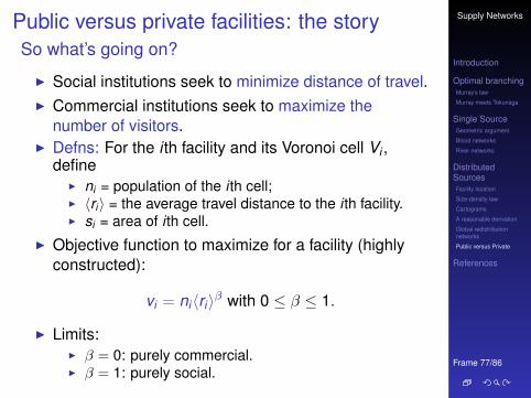
Supply Networks

Introduction




Blood networks

River networks


Size-density law

Cartograms




References

Frame 77/86

Public versus private facilities: the storySo what’s going on?

I Social institutions seek to minimize distance of travel.I Commercial institutions seek to maximize the

number of visitors.I Defns: For the i th facility and its Voronoi cell Vi ,

defineI ni = population of the i th cell;I 〈ri〉 = the average travel distance to the i th facility.I si = area of i th cell.

I Objective function to maximize for a facility (highlyconstructed):

vi = ni〈ri〉β with 0 ≤ β ≤ 1.

I Limits:I β = 0: purely commercial.I β = 1: purely social.

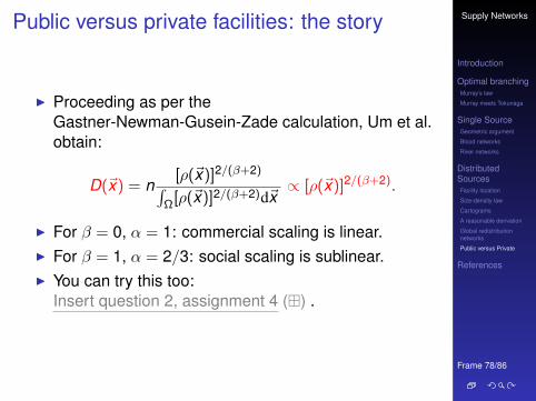
Supply Networks

Introduction




Blood networks

River networks


Size-density law

Cartograms




References

Frame 78/86

Public versus private facilities: the story

I Proceeding as per theGastner-Newman-Gusein-Zade calculation, Um et al.obtain:

D(~x) = n[ρ(~x)]2/(β+2)∫

Ω[ρ(~x)]2/(β+2)d~x∝ [ρ(~x)]2/(β+2).

I For β = 0, α = 1: commercial scaling is linear.I For β = 1, α = 2/3: social scaling is sublinear.I You can try this too:

Insert question 2, assignment 4 () .


Supply Networks

Introduction




Blood networks

River networks


Size-density law

Cartograms




References

Frame 79/86

References I

[1] J. R. Banavar, F. Colaiori, A. Flammini, A. Maritan,and A. Rinaldo.Topology of the fittest transportation network.Phys. Rev. Lett., 84:4745–4748, 2000. pdf ()

[2] J. R. Banavar, A. Maritan, and A. Rinaldo.Size and form in efficient transportation networks.Nature, 399:130–132, 1999. pdf ()

[3] S. Bohn and M. O. Magnasco.Structure, scaling, and phase transition in the optimaltransport network.Phys. Rev. Lett., 98:088702, 2007. pdf ()

[4] P. S. Dodds.Optimal form of branching supply and collectionnetworks.Phys. Rev. Lett., 104(4):048702, Jan 2010. pdf ()

http://www.uvm.edu/~pdodds/research/papers/others/2000/banavar2000a.pdf

http://www.uvm.edu/~pdodds/research/papers/others/1999/banavar1999a.pdf

http://www.uvm.edu/~pdodds/research/papers/others/2007/bohn2007a.pdf

http://www.uvm.edu/~pdodds/research/papers/others/2010/dodds2010a.pdf

Supply Networks

Introduction




Blood networks

River networks


Size-density law

Cartograms




References

Frame 80/86

References II[5] P. S. Dodds and D. H. Rothman.Geometry of river networks. I. Scaling, fluctuations,and deviations.Physical Review E, 63(1):016115, 2001. pdf ()

[6] M. T. Gastner and M. E. J. Newman.Diffusion-based method for producingdensity-equalizing maps.Proc. Natl. Acad. Sci., 101:7499–7504, 2004. pdf ()

[7] M. T. Gastner and M. E. J. Newman.Optimal design of spatial distribution networks.Phys. Rev. E, 74:016117, 2006. pdf ()

[8] M. T. Gastner and M. E. J. Newman.Shape and efficiency in spatial distribution networks.J. Stat. Mech.: Theor. & Exp., 1:P01015, 2006.pdf ()

http://www.uvm.edu/~pdodds/research/papers/others/2001/dodds2001a.pdf

http://www.uvm.edu/~pdodds/research/papers/others/2004/gastner2004a.pdf

http://www.uvm.edu/~pdodds/research/papers/others/2006/gastner2006c.pdf

http://www.uvm.edu/~pdodds/research/papers/others/2006/gastner2006a.pdf

Supply Networks

Introduction




Blood networks

River networks


Size-density law

Cartograms




References

Frame 81/86

References III

[9] S. M. Gusein-Zade.Bunge’s problem in central place theory and itsgeneralizations.Geogr. Anal., 14:246–252, 1982.

[10] K. A. McCulloh, J. S. Sperry, and F. R. Adler.Water transport in plants obeys Murray’s law.Nature, 421:939–942, 2003. pdf ()

[11] K. A. McCulloh, J. S. Sperry, and F. R. Adler.Murray’s law and the hydraulic vs mechanicalfunctioning of wood.Functional Ecology, 18:931–938, 2004. pdf ()

[12] C. D. Murray.The physiological principle of minimum work appliedto the angle of branching of arteries.J. Gen. Physiol., 9(9):835–841, 1926. pdf ()

http://www.uvm.edu/~pdodds/research/papers/others/2003/mcculloh2003a.pdf

http://www.uvm.edu/~pdodds/research/papers/others/2004/mcculloh2004a.pdf

http://www.uvm.edu/~pdodds/research/papers/others/1926/murray1926b.pdf

Supply Networks

Introduction




Blood networks

River networks


Size-density law

Cartograms




References

Frame 82/86

References IV

[13] C. D. Murray.The physiological principle of minimum work. I. Thevascular system and the cost of blood volume.Proc. Natl. Acad. Sci., 12:207–214, 1926. pdf ()

[14] C. D. Murray.A relationship between circumference and weight intrees and its bearing on branching angles.J. Gen. Physiol., 10:725–729, 1927. pdf ()

[15] I. Rodríguez-Iturbe and A. Rinaldo.Fractal River Basins: Chance and Self-Organization.Cambridge University Press, Cambrigde, UK, 1997.

[16] A. E. Scheidegger.Theoretical Geomorphology.Springer-Verlag, New York, third edition, 1991.

http://www.uvm.edu/~pdodds/research/papers/others/1926/murray1926a.pdf

http://www.uvm.edu/~pdodds/research/papers/others/1927/murray1927a.pdf

Supply Networks

Introduction




Blood networks

River networks


Size-density law

Cartograms




References

Frame 83/86

References V

[17] W. R. Stahl.Scaling of respiratory variables in mammals.Journal of Applied Physiology, 22:453–460, 1967.

[18] G. E. Stephan.Territorial division: The least-time constraint behindthe formation of subnational boundaries.Science, 196:523–524, 1977. pdf ()

[19] G. E. Stephan.Territorial subdivision.Social Forces, 63:145–159, 1984. pdf ()

[20] D. W. Thompson.On Growth and From.Cambridge University Pres, Great Britain, 2ndedition, 1952.

http://www.uvm.edu/~pdodds/research/papers/others/1977/stephan1977a.pdf

http://www.uvm.edu/~pdodds/research/papers/others/1984/stephan1984a.pdf

Supply Networks

Introduction




Blood networks

River networks


Size-density law

Cartograms




References

Frame 84/86

References VI

[21] D. W. Thompson.On Growth and Form — Abridged Edition.Cambridge University Press, Great Britain, 1961.

[22] D. L. Turcotte, J. D. Pelletier, and W. I. Newman.Networks with side branching in biology.Journal of Theoretical Biology, 193:577–592, 1998.

[23] J. Um, S.-W. Son, S.-I. Lee, H. Jeong, and B. J.Kim.Scaling laws between population and facilitydensities.Proc. Natl. Acad. Sci., 106:14236–14240, 2009.pdf ()

http://www.uvm.edu/~pdodds/research/papers/others/2009/um2009a.pdf

Supply Networks

Introduction




Blood networks

River networks


Size-density law

Cartograms




References

Frame 85/86

References VII

[24] P. D. Weinberg and C. R. Ethier.Twenty-fold difference in hemodynamic wall shearstress between murine and human aortas.Journal of Biomechanics, 40(7):1594–1598, 2007.pdf ()

[25] G. B. West, J. H. Brown, and B. J. Enquist.A general model for the origin of allometric scalinglaws in biology.Science, 276:122–126, 1997. pdf ()

[26] Q. Xia.The formation of a tree leaf.Submitted. pdf ()

http://www.uvm.edu/~pdodds/research/papers/others/2006/weinberg2006a.pdf

http://www.uvm.edu/~pdodds/research/papers/others/1997/west1997a.pdf

http://www.uvm.edu/~pdodds/research/papers/others/2007/xia2007a.pdf

Supply Networks

Introduction




Blood networks

River networks


Size-density law

Cartograms




References

Frame 86/86

References VIII

[27] Q. Xia.Optimal paths related to transport problems.Communications in Contemporary Mathematics,5:251–279, 2003. pdf ()

http://www.uvm.edu/~pdodds/research/papers/others/2003/xia2003a.pdf

optimal supply networks - uvm

Documents