Optimal percolation on multiplex networks

Saeed Osat,1 Ali Faqeeh,2 and Filippo Radicchi2

1Molecular Simulation Laboratory, Department of Physics, Faculty of Basic Sciences,Azarbaijan Shahid Madani University, Tabriz 53714-161, Iran

2Center for Complex Networks and Systems Research, School of Informatics and Computing,Indiana University, Bloomington, Indiana 47408, USA

Optimal percolation is the problem of finding the minimal set of nodes such that if the membersof this set are removed from a network, the network is fragmented into non-extensive disconnectedclusters. The solution of the optimal percolation problem has direct applicability in strategies ofimmunization in disease spreading processes, and influence maximization for certain classes of opin-ion dynamical models. In this paper, we consider the problem of optimal percolation on multiplexnetworks. The multiplex scenario serves to realistically model various technological, biological, andsocial networks. We find that the multilayer nature of these systems, and more precisely multiplexcharacteristics such as edge overlap and interlayer degree-degree correlation, profoundly changes theproperties of the set of nodes identified as the solution of the optimal percolation problem.

I. INTRODUCTION

A multiplex is a network where nodes are connectedthrough different types or flavors of pairwise edges [1–3]. A convenient way to think of a multiplex is as acollection of network layers, each representing a spe-cific type of edges. Multiplex networks are genuine rep-resentations for several real-world systems, including so-cial [4, 5], and technological systems [6, 7]. From a the-oretical point of view, a common strategy to understandthe role played by the co-existence of multiple networklayers is based on a rather simple approach. Given a pro-cess and a multiplex network, one studies the process onthe multiplex and on the single-layer projections of themultiplex (e.g., each of the individual layers, or the net-work obtained from aggregation of the layers). Recentresearch has demonstrated that accounting for or forget-ting about the effective co-existence of different types ofinteractions may lead to the emergence of rather differ-ent features, and have potentially dramatic consequencesin the ability to model and predict properties of the sys-tem. Examples include dynamical processes, such as dif-fusion [8, 9], epidemic spreading [10–13], synchroniza-tion [14], and controllability [15], as well as structuralprocesses such as those typically framed in terms of per-colation models [16–29].

The vast majority of the work on structural processeson multiplex networks have focused on ordinary perco-lation models where nodes (or edges) are considered ei-ther in a functional or in a non-functional state with ho-mogenous probability [30]. In this paper, we shift thefocus on the optimal version of the percolation process:we study the problem of identifying the smallest num-ber of nodes in a multiplex network such that, if thesenodes are removed, the network is fragmented into manydisconnected clusters of non-extensive size. We refer tothe nodes belonging to this minimal set as StructuralNodes (SNs) of the multiplex network. The solution ofthe optimal percolation problem has direct applicabilityin the context of robustness, representing the cheapest

way to dismantle a network [31–33]. The solution of theproblem of optimal percolation is, however, important inother contexts, being equivalent to the best strategy ofimmunization to a spreading process, and also to the beststrategy of seeding a network for some class of opinion dy-namical models [34–37]. Despite its importance, optimalpercolation has been introduced and considered in theframework of single-layer networks only recently [35, 36].The optimal percolation is an NP-complete problem [32].Hence, on large networks, we can only use heuristic meth-ods to find approximate solutions. Most of the researchactivity on this topic has indeed focused on the develop-ment of greedy algorithms [31–33, 35]. The generaliza-tion of optimal percolation to multiplex networks that weconsider here consists in the redefinition of the problemin terms of mutual connectedness [16]. To this end, wereframe several algorithms for optimal percolation fromsingle-layer to multiplex networks. Basically all the algo-rithms we use provide coherent solutions to the problem,finding sets of SNs that are almost identical. Our mainfocus, however, is not on the development of new algo-rithms, but on answering the following question: Whatare the consequences of neglecting the multiplex natureof a network under an optimal percolation process? Wecompare the actual solution of the optimal percolationproblem in a multiplex network with the solutions to thesame problem for single-layer networks extracted fromthe multiplex system. We show that “forgetting” aboutthe presence of multiple layers can be potentially danger-ous, leading to the overestimation of the true robustnessof the system mostly due to the identification of a veryhigh number of false SNs. We reach this conclusion witha systematic analysis of both synthetic and real multiplexnetworks.

II. METHODS

We consider a multiplex network composed of N nodesarranged in two layers. Each layer is an undirected andunweighted network. Connections of the two layers are

2

encoded in the adjacency matrices A and B. The genericelement Aij = Aji = 1 if nodes i and j are connectedin the first layer, whereas Aij = Aji = 0, otherwise.The same definition applies to the second layer, andthus to the matrix B. The aggregated network obtainedfrom the superposition of the two layers is character-ized by the adjacency matrix C, with generic elementsCij = Aij + Bij − AijBij . The basic objects we lookat are clusters of mutually connected nodes [16]: Twonodes in a multiplex network are mutually connected,and thus part of the same cluster of mutually connectednodes, only if they are connected by at least a path, com-posed of nodes within the same cluster, in every layer ofthe system. In particular, we focus our attention on thelargest among these cluster, usually referred to as theGiant Mutually Connected Cluster (GMCC). Our goal isto find the minimal set of nodes that, if removed fromthe multiplex, leads to a GMCC that has at maximuma size equal to

√N . This is a common prescription, yet

not the only one possible, to ensure that all clusters havenon-extensive sizes in systems with a finite number of ele-ments [35]. Whenever we consider single-layer networks,the above prescription apply to the single-layer clustersin the same exact way.

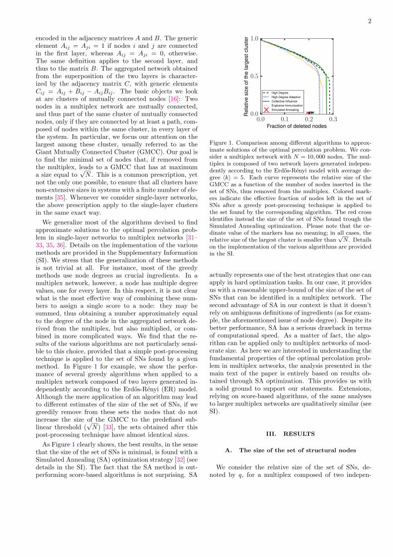
We generalize most of the algorithms devised to findapproximate solutions to the optimal percolation prob-lem in single-layer networks to multiplex networks [31–33, 35, 36]. Details on the implementation of the variousmethods are provided in the Supplementary Information(SI). We stress that the generalization of these methodsis not trivial at all. For instance, most of the greedymethods use node degrees as crucial ingredients. In amultiplex network, however, a node has multiple degreevalues, one for every layer. In this respect, it is not clearwhat is the most effective way of combining these num-bers to assign a single score to a node: they may besummed, thus obtaining a number approximately equalto the degree of the node in the aggregated network de-rived from the multiplex, but also multiplied, or com-bined in more complicated ways. We find that the re-sults of the various algorithms are not particularly sensi-ble to this choice, provided that a simple post-processingtechnique is applied to the set of SNs found by a givenmethod. In Figure 1 for example, we show the perfor-mance of several greedy algorithms when applied to amultiplex network composed of two layers generated in-dependently according to the Erdos-Renyi (ER) model.Although the mere application of an algorithm may leadto different estimates of the size of the set of SNs, if wegreedily remove from these sets the nodes that do notincrease the size of the GMCC to the predefined sub-linear threshold (

√N) [33], the sets obtained after this

post-processing technique have almost identical sizes.

As Figure 1 clearly shows, the best results, in the sensethat the size of the set of SNs is minimal, is found with aSimulated Annealing (SA) optimization strategy [32] (seedetails in the SI). The fact that the SA method is out-performing score-based algorithms is not surprising. SA

0.0 0.1 0.2 0.3Fraction of deleted nodes

0.0

0.5

1.0

Rel

ativ

esi

zeof

the

larg

estc

lust

er

High DegreeHigh Degree AdaptiveCollective InfluenceExplosive ImmunizationSimulated Annealing

Figure 1. Comparison among different algorithms to approx-imate solutions of the optimal percolation problem. We con-sider a multiplex network with N = 10, 000 nodes. The mul-tiplex is composed of two network layers generated indepen-dently according to the Erdos-Renyi model with average de-gree 〈k〉 = 5. Each curve represents the relative size of theGMCC as a function of the number of nodes inserted in theset of SNs, thus removed from the multiplex. Colored mark-ers indicate the effective fraction of nodes left in the set ofSNs after a greedy post-processing technique is applied tothe set found by the corresponding algorithm. The red crossidentifies instead the size of the set of SNs found trough theSimulated Annealing optimization. Please note that the or-dinate value of the markers has no meaning; in all cases, therelative size of the largest cluster is smaller than

√N . Details

on the implementation of the various algorithms are providedin the SI.

actually represents one of the best strategies that one canapply in hard optimization tasks. In our case, it providesus with a reasonable upper-bound of the size of the set ofSNs that can be identified in a multiplex network. Thesecond advantage of SA in our context is that it doesn’trely on ambiguous definitions of ingredients (as for exam-ple, the aforementioned issue of node degree). Despite itsbetter performance, SA has a serious drawback in termsof computational speed. As a matter of fact, the algo-rithm can be applied only to multiplex networks of mod-erate size. As here we are interested in understanding thefundamental properties of the optimal percolation prob-lem in multiplex networks, the analysis presented in themain text of the paper is entirely based on results ob-tained through SA optimization. This provides us witha solid ground to support our statements. Extensions,relying on score-based algorithms, of the same analysesto larger multiplex networks are qualitatively similar (seeSI).

III. RESULTS

A. The size of the set of structural nodes

We consider the relative size of the set of SNs, de-noted by q, for a multiplex composed of two indepen-

3

0.0 0.2 0.4 0.6 0.8 1.0Average degree

0.00

0.25

0.50

0.75

1.00

2 4 6 8 10 12 140.0

0.2

0.4

0.6

0.8R

elat

ive

size

ofth

est

ruct

ural

set

A

MultiplexLayer ALayer BAggregated

2 4 6 8 10 12 14

10−1

100

101

Rel

ativ

eer

ror

B

Ordinary perc. (layer A)Ordinary perc. (aggregated)

Figure 2. Optimal percolation problem in synthetic multiplexnetworks. A) We consider multiplex networks with N = 1, 000and layers generated independently according to the Erdos-Renyi model with average degree 〈k〉. We estimate the rela-tive size of the set of SNs on the multiplex as a function of 〈k〉(green circles), and compare with the same quantity but esti-mated on the individual layers (black squares, red down trian-gles) or the aggregated (orange right triangles). B) Relativeerrors of single-layer estimates of the size of the structural setwith respect to the ground-truth value provided by the multi-plex estimate. Colors and symbols are the same as those usedin panel A. The blue curves with no markers represent insteadthe results for an ordinary site percolation process [16].

dently fabricated ER network layers as a function of theiraverage degree 〈k〉. We compare the results obtained ap-plying the SA algorithm to the multiplex, namely qM ,with those obtained using SA on the individual lay-ers, i.e., qA and qB , or the aggregated network gener-ated from the superposition of the two layers, i.e., qS .By definition we expect that qM ≤ qA ' qB ≤ qS .What we don’t know, however, is how bad/good are themeasures qA, qB and qS in the prediction of the effec-tive robustness of the multiplex qM . For ordinary ran-dom percolation on ER multiplex networks with negli-gible overlap, we know that qM ' 1 − 2.4554/〈k〉 [16],qA ' qB ' 1−1/〈k〉, and qS ' 1−1/(2〈k〉) [38]. Relativeerrors are therefore εA ' εB ' (2.4554−1)/(〈k〉−2.4554),and εS ' (2.4554− 1/2)/(〈k〉− 2.4554). We find that therelative error for the optimal percolation behaves moreor less in the same way as that of the ordinary perco-lation (Figure 2B), noting that, as 〈k〉 is increased, thedecrease in the relative error associated with the individ-ual layers is slightly faster than what expected for theordinary percolation. The relative error associated withthe aggregated network is instead larger than the one ex-pected from the theory of ordinary percolation. As shownin Figure 2A, for sufficiently large 〈k〉, dismantling theER multiplex network is almost as hard as dismantlingany of its constituent layers.

B. Edge overlap and degree correlations

Next, we test the role played by edge overlap andlayer-to-layer degree correlation in the optimal perco-lation problem. These are ingredients that dramatically

0.0 0.5 1.0Relabeling probability

0.2

0.3

0.4

0.5

Rel

ativ

esi

zeof

the

stru

ctur

alse

t

MultiplexSingle layerAggregated

Figure 3. The effect of reducing edge overlaps and inter-layer degree-degree correlation by partially relabeling nodesin multiplex networks with initially identical layers. Initially,both layers are a copy of a random network generated by anErdos-Renyi model with N = 1, 000 nodes and average degree〈k〉 = 5. Then, in one of the layers, each node is selected toswitch its label with another randomly chosen node with acertain probability α. For each α, we determine the mean ofthe relative size of the set of SNs over 100 realizations of theSA algorithm on the multiplex network.

change the nature of the ordinary percolation transitionin multiplex networks [26, 39–43]. In Figure 3, we reportresults of a simple analysis. We take advantage of themodel introduced in Ref. [44], where a multiplex is con-structed with two identical layers. Nodes in one of thetwo layers relabeled with a certain probability α. Forα = 0, multiplex, aggregated network and single-layergraphs are all identical. For α = 1, the networks areanalogous to those considered in the previous section.We note that this model doesn’t allow to disentangle therole played by edge overlap among layers and the oneplayed by the correlation of node degrees. For α = 0,edge overlap amounts to 100%, and there is a one-to-onematch between the degree of a node in one layer and theother. As α increases, both edge overlap and degree cor-relation decrease simultaneously. As it is apparent fromthe results of Figure 3, the system reaches the multiplexregime for very small values of α, in the sense that therelative size of the set of SNs deviates instantly from itsvalue for α = 0. This is in line with what already foundin the context of ordinary percolation processes in mul-tiplex networks: as soon as there is a finite fraction ofedges that are not shared by the two layers, the systembehaves exactly as a multiplex [26, 39–43].

C. Accuracy and sensitivity

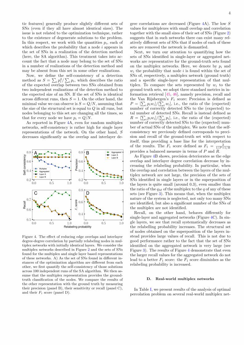
So far, we focused our attention only on the size of theset of SNs. We neglected, however, any analysis regardingthe identity of the nodes that actually compose this set.To proceed with such an analysis, we note that differentruns of the SA algorithm (or any algorithm with stochas-

4

tic features) generally produce slightly different sets ofSNs (even if they all have almost identical sizes). Theissue is not related to the optimization technique, ratherto the existence of degenerate solutions to the problem.In this respect, we work with the quantities pi, each ofwhich describes the probability that a node i appears inthe set of SNs in a realization of the detection method(here, the SA algorithm). This treatment takes into ac-count the fact that a node may belong to the set of SNsin a number of realizations of the detection method andmay be absent from this set in some other realizations.

Now, we define the self-consistency of a detectionmethod as S =

∑i p

2i /

∑i pi, which describes the ratio

of the expected overlap between two SNs obtained fromtwo independent realizations of the detection method tothe expected size of an SN. If the set of SNs is identicalacross different runs, then S = 1. On the other hand, theminimal value we can observe is S = Q/N , assuming thatthe size of the structural set is equal to Q in all runs, butnodes belonging to this set are changing all the times, sothat for every node we have pi = Q/N .

As reported in Figure 4A, even for random multiplexnetworks, self-consistency is rather high for single layerrepresentations of the network. On the other hand, Sdecreases significantly as the overlap and interlayer de-

0.0 0.2 0.4 0.6 0.8 1.0Relabeling probability

0.0

0.2

0.4

0.6

0.8

1.0

0.0 0.5 1.00.2

0.4

0.6

0.8

Sel

fcon

sist

ency

A

MultiplexAggregatedLayer ALayer B

0.0 0.5 1.00.2

0.4

0.6

0.8

Pre

cisi

on

B AggregatedLayer ALayer B

0.0 0.5 1.00.5

0.6

0.7

Rec

all

C

0.0 0.5 1.0

0.4

0.6

0.8

F1

scor

e

D

Figure 4. The effect of reducing edge overlaps and interlayerdegree-degree correlation by partially relabeling nodes in mul-tiplex networks with initially identical layers. We consider themultiplex networks described in Figure 2 and the sets of SNsfound for the multiplex and single layer based representationsof these networks. A) As the set of SNs found in different in-stances of the optimization algorithm are different from eachother, we first quantify the self-consistency of those solutionsacross 100 independent runs of the SA algorithm. We then as-sume that the multiplex representation provides the ground-truth classification of the nodes. We compare the results ofthe other representation with the ground truth by measuringtheir precision (panel B), their sensitivity or recall (panel C),and their F1 score (panel D).

gree correlations are decreased (Figure 4A). The low Svalues for multiplexes with small overlap and correlationtogether with the small sizes of their set of SNs (Figure 2)suggests that in such networks there can exist many rel-atively different sets of SNs that if nodes of each of thesesets are removed the network is dismantled.

Next, we turn our attention to quantifying how thesets of SNs identified in single-layer or aggregated net-works are representative for the ground-truth sets foundon the multiplex networks. Here, we denote by pi andwi the probability that node i is found within the set ofSNs of, respectively, a multiplex network (ground truth)and a specific single-layer representation of that mul-tiplex. To compare the sets represented by wi to theground truth sets, we adopt three standard metrics in in-formation retrieval [45, 46], namely precision, recall andthe Van Rijsbergen’s F1 score: Precision is defined asP = [

∑i piwi]/[

∑i wi], i.e., the ratio of the (expected)

number of correctly detected SNs to the (expected) to-tal number of detected SNs. Recall is instead defined asR = [

∑i piwi]/[

∑i pi], i.e., the ratio of the (expected)

number of correctly detected SNs to the (expected) num-ber of actual SNs of the multiplex. We note that the self-consistency we previously defined corresponds to preci-sion and recall of the ground-truth set with respect toitself, thus providing a base line for the interpretationof the results. The F1 score defined as F1 = 2

1/P+1/R

provides a balanced measure in terms of P and R.As Figure 4B shows, precision deteriorates as the edge

overlap and interlayer degree correlation decrease by in-creasing the relabeling probability. In particular, whenthe overlap and correlation between the layers of the mul-tiplex network are not large, the precision of the sets ofSNs identified in single layers or in the superposition ofthe layers is quite small (around 0.3), even smaller thanthe ratio of the qM of the multiplex to the q of any of thesesets (see Figure 3). This means that, when the multiplexnature of the system is neglected, not only too many SNsare identified, but also a significant number of the SNs ofthe multiplex are not identified.

Recall, on the other hand, behaves differently forsingle-layer and aggregated networks (Figure 4C). In sin-gle layers, we see that recall systematically decreases asthe relabelling probability increases. The structural setof nodes obtained on the superposition of the layers in-stead provides large values of recall. This is not due togood performance rather to the fact that the set of SNsidentified on the aggregated network is very large (seeFigure 3). The results of Figure 4 demonstrate that eventhe larger recall values for the aggregated network do notlead to a better F1 score: the F1 score diminishes as therelabeling probability is increased.

D. Real-world multiplex networks

In Table I, we present results of the analysis of optimalpercolation problem on several real-world multiplex net-

5

Network Layers NMultiplex Single layers Aggregate

qM S qA PA RA F(A)1

qB PB RB F(B)1

qS PS RS F(S)1

Air Transportation[26] American Air. – Delta 84 0.12 0.85 0.14 0.58 0.70 0.63 0.32 0.29 0.79 0.42 0.35 0.32 0.92 0.47

American Air. – United 73 0.10 0.99 0.16 0.32 0.52 0.40 0.14 0.68 1.00 0.81 0.25 0.39 1.00 0.56

United – Delta 82 0.10 1.00 0.27 0.23 0.62 0.34 0.12 0.80 1.00 0.89 0.33 0.30 1.00 0.46

C. Elegance[47, 48] Electric – Chem. Mon. 238 0.09 0.69 0.16 0.41 0.71 0.52 0.26 0.22 0.60 0.32 0.35 0.21 0.79 0.33

Electric – Chem. Pol. 252 0.12 0.79 0.15 0.50 0.63 0.56 0.39 0.24 0.78 0.37 0.45 0.22 0.82 0.35

Chem. Mon. – Chem. Pol. 259 0.25 0.82 0.28 0.69 0.77 0.73 0.39 0.51 0.79 0.62 0.42 0.48 0.80 0.60

Arxiv[49] physics.data-an – cond-mat.dis-nn 1400 0.05 0.78 0.10 0.38 0.77 0.51 0.07 0.55 0.75 0.63 0.13 0.31 0.81 0.45

physics.data-an – cond-mat.stat-mech 709 0.03 0.73 0.08 0.23 0.67 0.34 0.03 0.64 0.72 0.68 0.09 0.22 0.74 0.34

cond-mat.dis-nn – cond-mat.stat-mech 499 0.02 0.50 0.06 0.13 0.46 0.20 0.04 0.23 0.51 0.32 0.09 0.13 0.65 0.22

Drosophila M.[50, 51] Direct – Supp. Gen. 676 0.01 0.62 0.07 0.12 0.60 0.20 0.11 0.09 0.64 0.16 0.19 0.07 0.87 0.13

Direct – Add. Gen. 626 0.01 0.81 0.07 0.06 0.64 0.11 0.09 0.05 0.59 0.09 0.16 0.04 0.87 0.08

Supp. Gen. – Add. Gen. 557 0.09 0.82 0.14 0.44 0.74 0.55 0.12 0.50 0.70 0.58 0.20 0.35 0.80 0.49

Homo S.[48, 50] Direct – Supp. Gen. 4465 0.05 0.72 0.16 0.20 0.73 0.31 0.13 0.23 0.64 0.34 0.27 0.15 0.89 0.26

Physical – Supp. Gen. 5202 0.05 0.75 0.15 0.23 0.77 0.35 0.13 0.22 0.63 0.33 0.26 0.16 0.90 0.27

Table I. Optimal percolation in real multiplex networks. From left to right we report the following information. The firstthree columns contain the name of the system, the identity of the layers, and the number of nodes of the network. The fourthand fifth columns are results obtained from the optimal percolation problem studied on the multiplex network, and containinformation about the relative size qM , and self-consistency metric S of the set of SNs. Then, we report results obtained forthe first single-layer network of the multiplex, namely the fraction qA of nodes in the structural set, the precision PA, therecall RA, and the F1 score of the set of SNs of the first layer. The next three columns are identical to those, but refer to thesecond layer. Finally, the three rightmost columns contain information about the fraction qS of nodes in the structural set, PS

precision, RS recall, and the F1 score of the set of SNs for the aggregated network obtained from the superposition of the twolayers. All results have been obtained with 100 independent instances of the SA optimization algorithm.

works generated from empirical data. For most of thesenetworks, the optimal percolation on the multiplex rep-

Figure 5. Optimal percolation on the multiplex network ofUS domestic flights operated in January 2014 by AmericanAirlines and Delta. The red circles represent the nodes thatwere a member of the set of structural nodes in different real-izations of the optimal percolation on the multiplex represen-tation of the network. The size of each circle is proportional tothe probability of finding that node in the set of SNs. All otherairports in the multiplex are represented as black squares. In-terestingly, not all the 14 structural nodes match the top 14busiest hubs [52], nor the probabilities follow the same orderas the flight traffic of these airports. The results have been ob-tained with 100 independent instances of the SA optimizationalgorithm.

resentation has a rather high self-consistency. This im-plies that there is a certain small group of nodes thathave a major importance in the robustness of such real-world networks to the optimal percolation process. TheF1 score for most of the networks (not shown) is quite lowindicating that on real-world networks we loose essentialinformation about the optimal percolation problem if themultiplex structure is not taken into account.

To provide a practical case study with a lucid inter-pretation, we depict, in Figure 5, the results for opti-mal percolation on a multiplex network describing theair transportation operated by two of the major airlinesin the United States. SA identifies always 10 airports inthe set of SNs. There is a slight variability among differ-ent instances of the SA optimization, with a total of 14distinct airports appearing in the structural set at leastonce over 100 SA instances. However, changes in the SNset from run to run mostly regard airports in the same ge-ographical region. Overall, airports in the structural setare scattered homogeneously across the country, suggest-ing that the GMCC of the network mostly relies on hubsserving specific geographical regions, rather than globalhubs in the entire transportation system. For instance,the probabilities that describe the membership of the air-ports to the set of SNs do not strictly follow the same or-der as that of the recorded flight traffics [52]; nor merelythe number of connections of the airports (not shown) issufficient to determine the structural nodes. This is wellconsistent with the collective nature of the optimal per-colation on the complex network of air transportation.

6

IV. CONCLUSIONS

In this paper, we studied the optimal percolation prob-lem on multiplex networks. The problem regards the de-tection of the minimal set of nodes (or set of structuralnodes, SNs) such that if its members are removed fromthe network, the network is dismantled. The solution tothe problem provides important information on the mi-croscopic parts that should be maintained in a functionalstate to keep the overall system functioning, in a scenarioof maximal stress. Our study focused mostly on the char-acterization of the SN sets of a given multiplex network incomparison with those found on the single-layer projec-tions of the same multiplex, i.e., in a scenario where one“forgets” about the multiplex nature of the system. Ourresults demonstrate that, generally, multiplex networkshave considerably smaller sets of SNs compared to theSN sets of their single-layer based network representa-tions. The error committed when relying on single-layerrepresentations of the multiplex doesn’t regard only the

size of the SN sets, but also the identity of the SNs. Bothissues emerge in the analysis of synthetic network mod-els, where edge overlap and/or interlayer degree-degreecorrelations seem to fully explain the amount of discrep-ancy between the SN set of a multiplex and the SN setsof its single-layer based representations. The issues areapparent also in many of the real-world multiplex net-works we analyzed. Overall, we conclude that neglectingthe multiplex structure of a network system subjected tomaximal structural stress may result in significant inac-curacies about its robustness.

ACKNOWLEDGMENTS

AF and FR acknowledge support from the US ArmyResearch Office (W911NF-16-1-0104). FR acknowledgessupport from the National Science Foundation (GrantCMMI-1552487).

[1] S. Boccaletti, G. Bianconi, R. Criado, C. I. Del Ge-nio, J. Gomez-Gardenes, M. Romance, I. Sendina-Nadal,Z. Wang, and M. Zanin, Physics Reports 544, 1 (2014).

[2] M. Kivela, A. Arenas, M. Barthelemy, J. P. Gleeson,Y. Moreno, and M. A. Porter, Journal of complex net-works 2, 203 (2014).

[3] K.-M. Lee, B. Min, and K.-I. Goh, The European Phys-ical Journal B 88, 1 (2015).

[4] M. Szell, R. Lambiotte, and S. Thurner, Proceedingsof the National Academy of Sciences USA 107, 13636(2010).

[5] P. J. Mucha, T. Richardson, K. Macon, M. A. Porter,and J.-P. Onnela, science 328, 876 (2010).

[6] M. Barthelemy, Physics Reports 499, 1 (2011).[7] A. Cardillo, J. Gomez-Gardenes, M. Zanin, M. Romance,

D. Papo, F. del Pozo, and S. Boccaletti, Scientific Re-ports 3, 1344 (2013).

[8] S. Gomez, A. Dıaz-Guilera, J. Gomez-Gardenes, C. J.Perez-Vicente, Y. Moreno, and A. Arenas, Phys. Rev.Lett. 110, 028701 (2013).

[9] M. De Domenico, A. Sole-Ribalta, S. Gomez, andA. Arenas, Proc. Natl. Acad. Sci. USA 111, 8351 (2014).

[10] M. Dickison, S. Havlin, and H. E. Stanley, Phys. Rev. E85, 066109 (2012).

[11] A. Saumell-Mendiola, M. A. Serrano, and M. Boguna,Phys. Rev. E 86, 026106 (2012).

[12] C. Granell, S. Gomez, and A. Arenas, Phys. Rev. Lett.111, 128701 (2013).

[13] M. De Domenico, C. Granell, M. A. Porter, and A. Are-nas, Nature Physics (2016).

[14] C. I. del Genio, J. Gomez-Gardenes, I. Bonamassa, andS. Boccaletti, Science Adv. 2 (2016).

[15] M. Posfai, J. Gao, S. P. Cornelius, A.-L. Barabasi, andR. M. D’Souza, Phys. Rev. E 94, 032316 (2016).

[16] S. V. Buldyrev, R. Parshani, G. Paul, H. E. Stanley, andS. Havlin, Nature 464, 1025 (2010).

[17] R. Parshani, S. V. Buldyrev, and S. Havlin, Physicalreview letters 105, 048701 (2010).

[18] R. Parshani, C. Rozenblat, D. Ietri, C. Ducruet, andS. Havlin, EPL (Europhysics Letters) 92, 68002 (2011).

[19] G. Baxter, S. Dorogovtsev, A. Goltsev, and J. Mendes,Physical review letters 109, 248701 (2012).

[20] S. Watanabe and Y. Kabashima, Phys. Rev. E 89, 012808(2014).

[21] S.-W. Son, G. Bizhani, C. Christensen, P. Grassberger,and M. Paczuski, EPL (Europhysics Letters) 97, 16006(2012).

[22] B. Min, S. Do Yi, K.-M. Lee, and K.-I. Goh, PhysicalReview E 89, 042811 (2014).

[23] G. Bianconi, S. N. Dorogovtsev, and J. F. F. Mendes,Phys. Rev. E 91, 012804 (2015).

[24] G. Bianconi and S. N. Dorogovtsev, Physical Review E89, 062814 (2014).

[25] F. Radicchi and A. Arenas, Nature Physics 9, 717 (2013).[26] F. Radicchi, Nature Phys. 11, 597 (2015).[27] D. Cellai and G. Bianconi, Physical Review E 93, 032302

(2016).[28] G. Bianconi and F. Radicchi, Phys. Rev. E 94, 060301

(2016).[29] F. Radicchi and G. Bianconi, Phys. Rev. X 7, 011013

(2017).[30] D. Stauffer and A. Aharony, Introduction to percolation

theory (Taylor and Francis, 1991).[31] S. Mugisha and H.-J. Zhou, Phys. Rev. E 94, 012305

(2016).[32] A. Braunstein, L. DallAsta, G. Semerjian, and L. Zde-

borov, Proceedings of the National Academy of Sciences113, 12368 (2016).

[33] L. Zdeborova, P. Zhang, and H.-J. Zhou, Scientific Re-ports 6 (2016).

[34] F. Altarelli, A. Braunstein, L. Dall’Asta, andR. Zecchina, Phys. Rev. E 87, 062115 (2013).

7

[35] P. Clusella, P. Grassberger, F. J. Perez-Reche, andA. Politi, Phys. Rev. Lett. 117, 208301 (2016).

[36] F. Morone and H. A. Makse, Nature 524, 65 (2015).[37] S. Pei, X. Teng, J. Shaman, F. Morone, and H. A. Makse,

arXiv preprint arXiv:1606.02739 (2016).[38] M. Molloy and B. Reed, Random structures & algorithms

6, 161 (1995).[39] D. Cellai, E. Lopez, J. Zhou, J. P. Gleeson, and G. Bian-

coni, Physical Review E 88, 052811 (2013).[40] G. Bianconi, Physical Review E 87, 062806 (2013).[41] B. Min, S. Lee, K.-M. Lee, and K.-I. Goh, Chaos, Soli-

tons & Fractals 72, 49 (2015).[42] G. J. Baxter, G. Bianconi, R. A. da Costa, S. N. Doro-

govtsev, and J. F. Mendes, Physical Review E 94, 012303(2016).

[43] D. Cellai, S. N. Dorogovtsev, and G. Bianconi, PhysicalReview E 94, 032301 (2016).

[44] G. Bianconi and S. N. Dorogovtsev, arXiv preprintarXiv:1411.4160 (2014).

[45] W. Chu and T. Y. Lin, Foundations and advances indata mining , Vol. 180 (Springer-Verlag, Berlin Heidel-berg, 2005).

[46] G. Maino and G. L. Foresti, Image Analysis and Pro-cessing – ICIAP 2011 , Vol. 6979 (Springer-Verlag, BerlinHeidelberg, 2011).

[47] B. L. Chen, D. H. Hall, and D. B. Chklovskii, Proceed-ings of the National Academy of Sciences of the UnitedStates of America 103, 4723 (2006).

[48] M. De Domenico, M. A. Porter, and A. Arenas, Journalof Complex Networks , cnu038 (2014).

[49] M. De Domenico, A. Lancichinetti, A. Arenas, andM. Rosvall, Physical Review X 5, 011027 (2015).

[50] C. Stark, B.-J. Breitkreutz, T. Reguly, L. Boucher,A. Breitkreutz, and M. Tyers, Nucleic acids research34, D535 (2006).

[51] M. De Domenico, V. Nicosia, A. Arenas, and V. Latora,Nature communications 6 (2015).

[52] Wikipedia, List of the busiest airports in the UnitedStates.

1

Optimal percolation on multiplex networks

Saeed Osat, Ali Faqeeh, Filippo Radicchi

Supplementary Information

CONTENTS

S.1. Dismantling Algorithms 1A. High Degree (HD) 2B. High Degree Adaptive (HDA) 3C. Collective Influence (CI) 4D. Explosive Immunization (EI) 5E. Simulated Annealing (SA) 8

S.2. Greedy Reinserting (GR) 9

S.3. Complementary results for the degree-based methods 10

References 12

S.1. DISMANTLING ALGORITHMS

In this section, we briefly discuss some of the most effective dismantling algorithms on

monoplex networks and their generalization to multiplex networks with two layers. The aim

of these algorithms is to approximate the set of structural nodes which is the minimal set

of nodes that their removal dismantles the network into vanishingly small (non-extensive)

clusters. We first introduce some of the score-based algorithms. In such algorithms, at each

step, a score for each node is calculated and the node with the highest score is removed

(when several nodes have the same score, one of them is removed at random). We discuss

four different types of such algorithms: High Degree (HD), High Degree Adaptive (HDA),

Collective Influence (CI) and Explosive Immunization (EI). These methods are partially

deterministic in nature, i.e., nearly the same set of structural nodes are discovered at each

realizations of the algorithm. Besides score-based algorithms, we present Simulated An-

nealing (SA) algorithm which is a greedy algorithm that searches the solution space of the

dismantling problem to find the best approximation to the structural sets. The SA method

takes into account the collective behavior of the dismantling problem and provides several

dismantling sets for different realizations of the algorithm on the same network structure.

2

A. High Degree (HD)

In a monoplex network, the easiest way to dismantle a network, is a degree-based attack.

After sorting the nodes with respect to their degrees, the nodes with the highest degree are

removed one by one1 until the network is dismantled. As this algorithm is deterministic

(except from the randomness in choosing a node from those with the same degree), the set

of nodes that are removed to dismantle the network is almost unique.

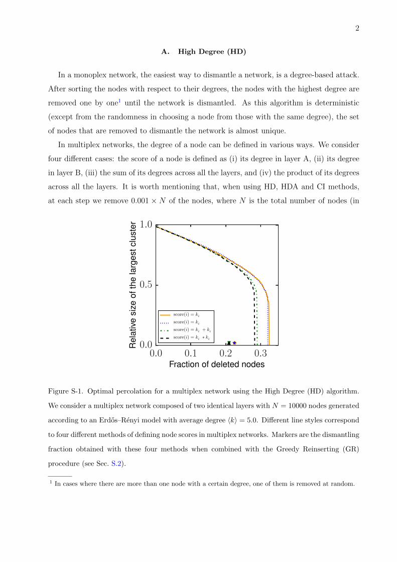
In multiplex networks, the degree of a node can be defined in various ways. We consider

four different cases: the score of a node is defined as (i) its degree in layer A, (ii) its degree

in layer B, (iii) the sum of its degrees across all the layers, and (iv) the product of its degrees

across all the layers. It is worth mentioning that, when using HD, HDA and CI methods,

at each step we remove 0.001 × N of the nodes, where N is the total number of nodes (in

0.0 0.1 0.2 0.3Fraction of deleted nodes

0.0

0.5

1.0

Rel

ativ

esi

zeof

the

larg

estc

lust

er

score(i) = kAi

score(i) = kBi

score(i) = kAi + kB

i

score(i) = kAi ∗ kB

i

Figure S-1. Optimal percolation for a multiplex network using the High Degree (HD) algorithm.

We consider a multiplex network composed of two identical layers with N = 10000 nodes generated

according to an Erdos–Renyi model with average degree 〈k〉 = 5.0. Different line styles correspond

to four different methods of defining node scores in multiplex networks. Markers are the dismantling

fraction obtained with these four methods when combined with the Greedy Reinserting (GR)

procedure (see Sec. S.2).

1 In cases where there are more than one node with a certain degree, one of them is removed at random.

3

each layer) of the multiplex.

As Figure S-1 illustrates, to destruct a multiplex, the two scores defined as a combination

of degrees in different layers are more effective than those based on the degrees in only one

of the layers. In the main script and in the rest of the Supplemental Material (SM) when we

refer to HD method, we mean the one in which a node degree is the product of its degrees

across all the layers.

B. High Degree Adaptive (HDA)

In the HD algorithm if we take into account the history of the process and recalculate, at

each step, the degrees of the nodes, it is referred to as an HDA algorithm. Since the HDA

algorithm is adaptive it is expected to work better than the HD method. In each step of the

monoplex version of the HDA, we remove a fraction 0.001 × N of the nodes that had the

highest degrees; then we recalculate the degree of the nodes present in the Giant Connected

Component (GCC) of the network. We repeat this process until the size of the GCC reduces

to√N or smaller; this threshold satisfies the condition that in the dismantled network the

size of all the clusters is a sub-linear function of N .

0.0 0.1 0.2 0.3Fraction of deleted nodes

0.0

0.5

1.0

Rel

ativ

esi

zeof

the

larg

estc

lust

er

score(i) = kAi

score(i) = kBi

score(i) = kAi + kB

i

score(i) = kAi ∗ kB

i

Figure S-2. Performance of the HDA method on the same multiplex network considered in Fig-

ure S-1. Four different plots correspond to four different type of defining the degree of a node.

4

Like the HD case, we can define at least four methods to define the degree of a node.

Please notice that in the multiplex version, when we update the degrees, we exclude those

neighbors that are not in the Giant Mutually Connected Component (GMCC) of the net-

work. Figure S-2 shows the effectiveness of the HDA algorithm for the different definitions

of nodes’ degrees. Similar to the results for HD, it is more effective to combine the scores of

different layers, than considering layers as isolated networks. In all the subsequent sections

and in the main script, when we refer to HDA, we mean the one in which the score of a

node is defined as the multiplication of its degrees across all the layers.

C. Collective Influence (CI)

In the monoplex version of the CI algorithm [S1], the score CIi(l) of node i is equal to the

excess degree of i multiplied by the sum of the excess degrees of its neighbours at a specific

distance l from i:

CIi(l) = (ki − 1)∑

j∈∂Ball(i,l)

(kj − 1), (S.1)

where ∂Ball(i, l) denotes the neighbors of i at the distance l (i.e., the nodes that have a

geodesic distance l from i). At each step, the CI score is adaptively calculated for all the

0.0 0.1 0.2 0.3Fraction of deleted nodes

0.0

0.5

1.0

Rel

ativ

esi

zeof

the

larg

estc

lust

er

CIi = CIAi

CIi = CIBi

CIi = CIAi + CIB

i

CIi = CIAi ∗ CIB

i

Figure S-3. The performance of the CI algorithm with l = 4 on the network of Figure S-1 using

different definitions for the collective influence of a node.

5

nodes; then nodes with the highest score are removed from the network, until the network

is dismantled. It was shown [S1, S2] that the performance of the CI method increases with

l up to l = 4; for l > 4 the performance is not improved appreciably as l is increased.

To adapt the CI algorithm to multiplex networks with two layers, we considered several

possible definitions of the CI score in the multiplex: (i) using the CI obtained based only on

the structure of layer A, (ii) based only on the structure of layer B, (iii) the sum of the CIs

of a node in layer A and layer B, and (iv) the product of these two CI scores. Figure S-3

illustrates that, the generalizations of the CI method we considered here are not as effective

as those derived based on the HD (Figure S-1) and HDA (Figure S-2) methods. Thus,

methods based on the CI measures of the layers do not provide an effective algorithm for

the optimal percolation problem.

D. Explosive Immunization (EI)

The EI algorithm is based on a method referred to as explosive percolation. The original

explosive percolation method was introduced by Achlioptas et al. [S3]. In this method at

first all the edges are removed; then they are gradually reintroduced to the network, but in

a specific order that prevents the formation of the GCC, until a point where the formation

of the GCC is inevitable. To add a new edge, first several random edges are selected. Then

a score is calculated for each of the selected edges using a predefined kernel2. Then the edge

with the minimum score is added back the network. The scores represent the contribution of

each edge in the formation of the giant cluster. When the network reaches the point where

the formation of the giant cluster is inevitable, the rest of the edges are added back using

the same kernel.

A problem related to explosive percolation is the optimal immunization [S4] in which the

goal is to find the blocker nodes, which if get vaccinated, the giant connected component of

the susceptible nodes breaks down; this break down eliminates a large scale epidemic spread.

Clusella et al. [S4] proposed a reverse approach to find the blockers. They introduced an

algorithm that locates instead all the nodes that are irrelevant to the formation of the giant

susceptible cluster. In this respect, their algorithm is a modified version of the explosive per-

2 A possible kernel, for example, defines the score as the sum of the sizes of the two clusters connected by

the corresponding edge.

6

colation. Their algorithm considers the site percolation version of the explosive percolation,

in which all the links are present but, in the beginning, all the nodes are absent. Then, all

the non-blocker nodes (that have no contribution to the formation of the giant susceptible

cluster) are added gradually. The remaining nodes are the blocker nodes which should be

vaccinated. We refer to this method as the explosive immunization (EI) algorithm.

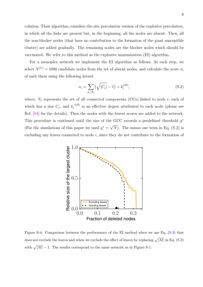
For a monoplex network we implement the EI algorithm as follows. At each step, we

select N (C) = 1000 candidate nodes from the set of absent nodes, and calculate the score σi

of each them using the following kernel:

σi =∑

j⊂Ni

(√|Cj| − 1

)+ k

(eff)i , (S.2)

where, Ni represents the set of all connected components (CCs) linked to node i, each of

which has a size Cj, and k(eff)i is an effective degree attributed to each node (please see

Ref. [S4] for the details). Then the nodes with the lowest scores are added to the network.

This procedure is continued until the size of the GCC exceeds a predefined threshold g∗

(For the simulations of this paper we used g∗ =√N). The minus one term in Eq. (S.2) is

excluding any leaves connected to node i, since they do not contribute to the formation of

0.0 0.1 0.2 0.3Fraction of deleted nodes

0.0

0.5

1.0

Rel

ativ

esi

zeof

the

larg

estc

lust

er

Excluding leavesIncluding leaves

Figure S-4. Comparison between the performance of the EI method when we use Eq. (S.3) that

does not exclude the leaves and when we exclude the effect of leaves by replacing√|M | in Eq. (S.3)

with√|M | − 1. The results correspond to the same network as in Figure S-1.

7

the GCC and should be ignored in the score of a node.

In our extension of the EI method to multiplex networks, we consider the different kernel

but otherwise perform the exact same procedure as the one described above. The new kernel

(Eq. (S.3)) we use is based on the sizes of the mutually connected components (MCCs) rather

than on the sizes of CCs:

σi = 1/2

[ ∑

j⊂N [A]i

(√|Mj|

)+∑

j⊂N [B]i

(√|Mj|

)]+

√k

[A](eff)i k

[B](eff)i , (S.3)

where N[A]i is the set of neighbors of node i in layer A, Mj is the size of the MCC to which

node j belongs, and k[A](eff)i is the effective degree of i in layer A obtained using the same

definition proposed [S4] for the monoplex version of the EI method.

In Eq. (S.3) we do not add a minus 1 term to exclude the leaves; the reason is that

while in monoplex networks leaves do not have a significant contribution in the formation

of the GCC, in multiplex networks even a leaf node is important in the formation of the

GMCC. This is because at the sub-critical regime of multiplex networks usually most of the

MCCs are isolated nodes or have very small sizes. Figure S-4 certifies that if the leaves were

excluded instead, the performance of the algorithm would decrease. Figure S-5 shows that

the performance of the EI method does not depend appreciably on the number of candidate

0.0 0.1 0.2 0.3Fraction of deleted nodes

0.0

0.5

1.0

Rel

ativ

esi

zeof

the

larg

estc

lust

er

N (C) = 500

N (C) = 1000

N (C) = 5000

N (C) = 10000

Figure S-5. The results of the EI method do not depend appreciably on the number of candidate

nodes N (C). The simulations are performed on the same network used in Figure S-1.

8

nodes (N (C)). In the simulations of Figure 1 of the main text, we used a N (C) = 1000.

E. Simulated Annealing (SA)

The simulated annealing (SA) method has been used for the dismantling problem in

monoplex networks [S5]. Generally an SA algorithm defines an energy function that at-

tributes energy values to each configuration of the system. The phase space of the system

is searched for the optimal configuration (the one with the minimum energy) by Markov

Chain Monte Carlo moves that switch the system from one configuration to another. In dis-

mantling of multiplex networks, the algorithm should find the minimal set of nodes which if

deleted the size of the GMCC becomes non-extensive. Each configuration of the multiplex

network is represented by {R, g}, where R and g are, respectively, the number of removed

nodes (each node and all its corresponding replica nodes are counted as one node), and the

relative size of the GMCC. The energy of a configuration is defined as follows:

ε = Rv + g, (S.4)

where v is the cost of removing a node from the multiplex network and in the simulations

presented in this paper it is set v = 0.6. At each step t of the algorithm, one node, present or

removed, is selected at random; then one of the following sets of operations are performed:

• If the node is present and it belongs to the GMCC, it is removed (thus Rt = Rt−1 + 1)

and the new size of the GMCC (gt) is calculated.

• If the node is present but it does not belong to the GMCC, then it is removed (thus

Rt = Rt−1 + 1); but since it did not belong to the GMCC, gt = gt−1.

• If the node is in the set of removed nodes, it is added back to the network and Rt =

Rt−1 − 1. Then Mi (the size of the MCC formed after inserting i) is calculated and

gt = max (Mi, gt−1).

Afterwards the energy of the new configuration εt is calculated and the set of operations is

accepted with a probability equal to min(1, e−β(εnew−ε)

). If it is accepted, the new configu-

ration ({Rt, gt}) is retained, otherwise, the operations are omitted and the old configuration

({Rt−1, gt−1}) is preserved.

Here, β is interpreted as the inverse of the temperature of the annealing process. The SA

algorithm starts with a βmin and, at each step, β is slightly increased by δβ. A smaller δβ

9

means a slower decrease in the temperature which allows the SA method to better search for

the optimal configurations, at the expense of increasing the running time of the algorithm.

In this paper we change the values of β from 0.5 to 20.0 with δβ = 10−6.

In Figure 1 of the main text, we show that the SA method outperforms the four score-

based algorithms; thus, for the analysis of the optimal percolation problem, we mostly use

the SA method (see the main text). In Sec. S.3, we also provide results for the second best

algorithm, i.e., the HDA method and show that the results are qualitatively similar to those

of the SA method.

S.2. GREEDY REINSERTING (GR)

After a network (either isolated or multiplex) is dismantled using a greedy or score-based

algorithm, there are some removed nodes that if added back to the network, the size of

the GMCC is not increased substantially, i.e., no cluster with an extensive size is created

if they are reinserted. Such nodes may have been removed because the greedy or score-

based algorithms are not exact in the sense that they do not take into account the collective

nature of the dismantling problem. An approach that addresses this issue is referred to as

the greedy reinserting (GR) method [S2, S5]. In the GR method, after a set of structural

nodes is detected using another algorithm, at each step a randomly chosen node from the

set is reinserted to the network, and unless its reinsertion does not increase the size of the

GMCC to a threshold√N , it is removed again. This process is continued until practically

none of the nodes remained in the set can be added to the network without keeping the size

of the GMCC non-extensive.

As shown in Figures S-1–S-5 and Figure 1 of the main text, the GR method boosts effec-

tively the performance of every one of the score-based dismantling algorithms and returns

sets of structural nodes with almost identical sizes irrespective of the initial algorithm used.

Moreover, the result of each of the score-based algorithms combined with the GR method is

nearly as good as that of the SA method (the SA method itself is not improved appreciably

by applying a GR method afterwards). These results suggest that probably the sets obtained

by the SA method and any one of the score-based algorithms combined with GR are to a

considerable extent similar to each other. In Sec. S.3 we show that actually the results of

HDA and those of SA are qualitatively similar.

10

S.3. COMPLEMENTARY RESULTS FOR THE DEGREE-BASED METHODS

In this section, we provide further results for the HD (Figure S-6) and the HDA (Figure S-

7) methods, and also for the combination of the GR method with HDA (Figures S-8–S-9);

we compare these results with some of the results of the SA algorithm presented in the

main text. In contrast to the SA algorithm, the degree-based algorithms are much more

efficient in terms of the running time; hence, we were able to produce some of the results

(see Figures S-6–S-7) for larger ER networks.

Figures S-6 and S-7 show that, for both HD and HDA performed on the aggregated

representation, the behavior of qc (the relative size of the set of structural nodes) with

0.0 0.2 0.4 0.6 0.8 1.0Average degree

0.0

0.2

0.4

0.6

0.8

1.0

2 4 6 8 10 12 140.0

0.2

0.4

0.6

0.8

Rel

ativ

esi

zeof

the

stru

ctur

alse

t

A

MultiplexLayer ALayer BAggregated

2 4 6 8 10 12 14

10−1

100

101R

elat

ive

erro

r

B

Ordinary perc. (layer A)Ordinary perc. (aggregated)

Figure S-6. Like Figure 2 of the main script. Dismantling of a multiplex network with each layer

generated independently according to the Erdos-Renyi model with average degree 〈k〉 and N = 105

using the HD method.

0.0 0.2 0.4 0.6 0.8 1.0Average degree

0.0

0.2

0.4

0.6

0.8

1.0

2 4 6 8 10 12 140.0

0.2

0.4

0.6

0.8

Rel

ativ

esi

zeof

the

stru

ctur

alse

t

A

MultiplexLayer ALayer BAggregated

2 4 6 8 10 12 14

10−1

100

101

Rel

ativ

eer

ror

B

Ordinary perc. (layer A)Ordinary perc. (aggregated)

Figure S-7. Like Figure S-6, for the HDA algorithm.

11

0.0 0.5 1.0Relabeling probability

0.2

0.3

0.4

0.5

Rel

ativ

esi

zeof

the

stru

ctur

alse

t

MultiplexSingle layerAggregated

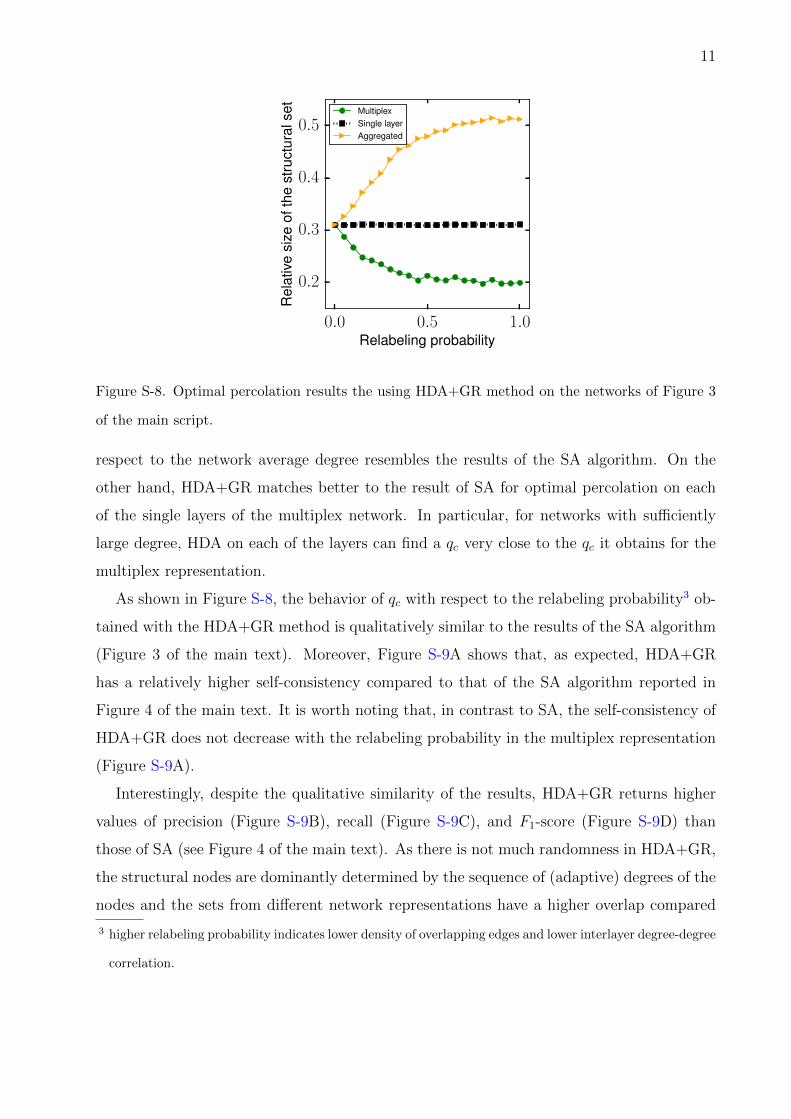
Figure S-8. Optimal percolation results the using HDA+GR method on the networks of Figure 3

of the main script.

respect to the network average degree resembles the results of the SA algorithm. On the

other hand, HDA+GR matches better to the result of SA for optimal percolation on each

of the single layers of the multiplex network. In particular, for networks with sufficiently

large degree, HDA on each of the layers can find a qc very close to the qc it obtains for the

multiplex representation.

As shown in Figure S-8, the behavior of qc with respect to the relabeling probability3 ob-

tained with the HDA+GR method is qualitatively similar to the results of the SA algorithm

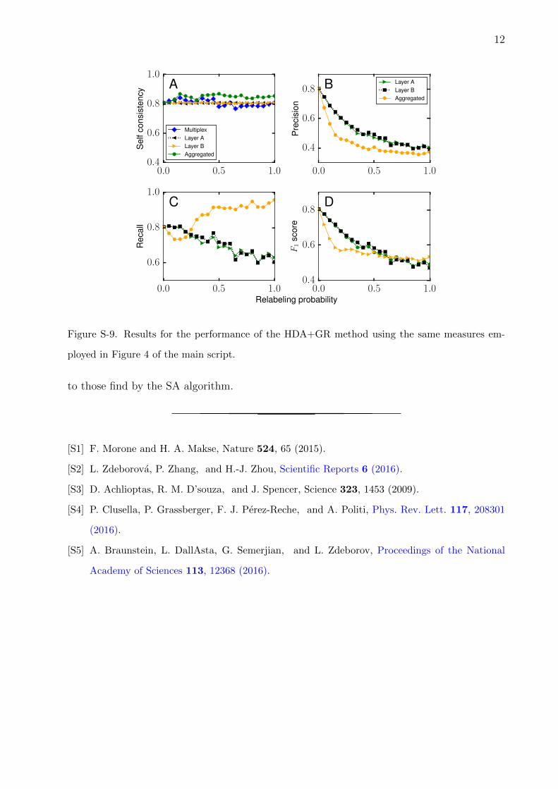
(Figure 3 of the main text). Moreover, Figure S-9A shows that, as expected, HDA+GR

has a relatively higher self-consistency compared to that of the SA algorithm reported in

Figure 4 of the main text. It is worth noting that, in contrast to SA, the self-consistency of

HDA+GR does not decrease with the relabeling probability in the multiplex representation

(Figure S-9A).

Interestingly, despite the qualitative similarity of the results, HDA+GR returns higher

values of precision (Figure S-9B), recall (Figure S-9C), and F1-score (Figure S-9D) than

those of SA (see Figure 4 of the main text). As there is not much randomness in HDA+GR,

the structural nodes are dominantly determined by the sequence of (adaptive) degrees of the

nodes and the sets from different network representations have a higher overlap compared

3 higher relabeling probability indicates lower density of overlapping edges and lower interlayer degree-degree

correlation.

12

0.0 0.2 0.4 0.6 0.8 1.0Relabeling probability

0.0

0.2

0.4

0.6

0.8

1.0

0.0 0.5 1.00.4

0.6

0.8

1.0

Sel

fcon

sist

ency

A

MultiplexLayer ALayer BAggregated

0.0 0.5 1.0

0.4

0.6

0.8

Pre

cisi

on

B Layer ALayer BAggregated

0.0 0.5 1.0

0.6

0.8

1.0

Rec

all

C

0.0 0.5 1.00.4

0.6

0.8

F1

scor

e

D

Figure S-9. Results for the performance of the HDA+GR method using the same measures em-

ployed in Figure 4 of the main script.

to those find by the SA algorithm.

[S1] F. Morone and H. A. Makse, Nature 524, 65 (2015).

[S2] L. Zdeborova, P. Zhang, and H.-J. Zhou, Scientific Reports 6 (2016).

[S3] D. Achlioptas, R. M. D’souza, and J. Spencer, Science 323, 1453 (2009).

[S4] P. Clusella, P. Grassberger, F. J. Perez-Reche, and A. Politi, Phys. Rev. Lett. 117, 208301

(2016).

[S5] A. Braunstein, L. DallAsta, G. Semerjian, and L. Zdeborov, Proceedings of the National

Academy of Sciences 113, 12368 (2016).