optimal sizing of grid tied solar pv for transmission ... · congested power systems using facts...

International Journal of Applied Engineering Research ISSN 0973-4562 Volume 14, Number 17 (2019) pp. 3598-3609

© Research India Publications. http://www.ripublication.com

3598

Optimal Sizing of Grid-Tied Solar PV for Transmission Congestion Management

in a Deregulated System using LMP Analysis

Malado Diallo.1*, Livingstone Ngoo.2, Michael Saulo.3, and Benaissa Bekkouche.4

1Department of Electrical Engineering, Pan African University, Institute for Basic Sciences, Technology and Innovation, Kenya. 2Department of Electrical Engineering, Multimedia University of Technology, Kenya.

3Department of Electrical Engineering, Technical University of Mombasa, Mombasa, Kenya. 4Department of Renewable Energy and Sustainable Development, University of Mostaganem, Algeria.

*Corresponding author

Abstract

In deregulated power system, it is desired to transmit power to

every part of the network without any limits resulting from

congestion and as a result avoiding inefficiencies in generation

dispatch. In order to reduce congestion in the transmission lines,

a new approach to manage transmission congestion and

improve social welfare is proposed in this research. This

approach consists of optimal sizing and placement of grid-tied

solar PV system using LMP analysis for congestion

management and maximization of social welfare. The LMP and

congestion rent (CR) at each node of the system are obtained

from the Lagrange multiplier associated with OPF formulation

to determine the optimal location of solar power plant. With

optimal sizing and placement, a grid-tied solar PV system has

the ability to reduce power losses, improve voltage profile and

power quality. Since solar power is a random and intermittent

energy, the sizing of solar PV system is done by taking into

account the power variation of the solar system. The results

show that the proposed approach gives better results, reduced

congestion in the system while maximizing social welfare is.

The proposed methods are implemented on the modified IEEE

30-bus test system.

Keywords: Locational marginal pricing (LMP); social welfare

(SW); congestion rent (CR) congestion management; solar PV;

optimal power flow (OPF).

I. INTRODUCTION

In a deregulated power system, one drawback of transmission

network is overloading. It is desirable to be able to transmit

power to all parts of network without violating system security

constraints. The electrical power that can be transmitted

between two locations in a network is limited by several

security criteria such as voltage limits, lines thermal limits and

stability limits [1]. When power cannot be transmitted to parts

of network because of the limits mentioned, the system is said

to be congested [2].

Transmission congestion is a major problem and can lead to

serious disruptions in the power system. Congestion is due to

poor coordination between generation and transmission

services and sudden increase in load demand. This increases the

gap between supply and demand thus affecting social welfare

negatively. Therefore, Transmission congestion has impact on

the entire system as well as on the individual market

participants i.e., sellers and buyers [3] [4]. Solutions to relieve

congestion, generally referred to as congestion management

schemes, are of interest to both system operators and planners

[5]. One of the most important functions of independent system

operators ("ISO") in the deregulated electrical system is

congestion management.

Several methods have been proposed in the literature for

congestion management. In [6], the proposed method for

congestion management determines the optimal location of a

distributed generator (DG) in a deregulated electrical grid using

the basis of a bus impedance matrix (Z-bus-based contribution

factors). According to [7], congestion can be alleviated by

rescheduling the timing of actual emissions of generator energy,

limiting the load and operating phase shifters or FACTS

devices [7]. A congestion management technique integrating

wind energy has been proposed in which the independent grid

operator (ISO) is responsible for proposing the appropriate size

and location for the implementation of the wind farm on the

basis of the LMP price reduction [5]. An enhanced Shift Load

Factor (SLF) based Line Outage Distribution Factor (LODF)

LMP congestion management technique has been presented in

paper [8]. The following paper [9] investigates the cost control

problem of congestion management model Based on Ant

Colony Algorithm in the real-time power systems. It is show



3599

that the model can significantly reduce the cost of electricity.

Conventional optimization methods are used to manage

congested power systems using FACTS devices as an

alternative to efficiently minimize the power flows in the

system especially during the heavy demands [10]. The use of

FACTS devices helps improve power capability, lower system

losses, and increase system stability by controlling power flows

[10]. The literature [11] proposed a congestion management

technique called DG based on Locational Marginal Price (LMP)

schemes. This method places DG in the system to relieve

congestion and minimizes generation costs.

In this paper, locational marginal price (LMP) will be used to

determine the optimal location of grid-tied solar PV in a

deregulated power system. The LMP of a site is defined as the

marginal cost to provide an additional increase in MW capacity

at the site without violating the safety limits of the system. This

price reflects not only the marginal cost of energy production,

but also its delivery. Due to the effects of transmission losses

and congestion on the transmission system, LMPs can vary

considerably from one place to another. The LMP is the sum

of marginal energy costs, marginal losses and congestion [4].

The persistence of the congestion problem indicates that new

generation capacity or additional transmission facilities are

needed to manage congestion. Decentralised production

sources or renewable energies can be of great value in a highly

congested area where LMPs are higher than elsewhere [12].In

this study, we use LMP analysis and congestion rent to locate

the optimal placement of the solar power plant to relieve

congestion in transmission line. While the installation of solar

power plant at an optimal location in the congested system

could effectively improve the voltage profile, power quality

and reliability of the grid, it also ensures the maximization of

social welfare and congestion management.

With regard to the sizing of solar power plant, a new challenge

arises: the random and intermittent nature of solar power due to

constant variation of irradiance and temperature. This means

that the determined size of the solar power plant is actually the

required output power from the point of view of the power

system. However, the actual capacity of the solar power plant

is not simply the same as the determined size. It is proposed

here to calculate the actual capacity of the solar power plant

based on probability density function methods (PDF). The

proposed approach is evaluated in IEEE 30-bus test system.

The rest of the document is organized as follows. The problem

formulation of the proposed approach is described in Section 2.

The methodology is described in section 3. The optimal size

and location of the solar power plant for congestion

management are calculated for a test system in section 4. The

main contributions of this document are summarized in section

5.

II. PROBLEM FORMULATION

2. 1. Problem formulation of social welfare

maximization without solar power

The objective of power systems operation and planning in

deregulated power markets is to maximize the social welfare

through minimizing total generation costs [13]. The social

welfare (SW) is obtained as the benefit function 𝐵𝐷𝑖(𝑃𝐷𝑖) in

$/hr of DISCOs/DSTs minus the cost function 𝐶𝐺𝑖(𝑃𝐺𝑖) in $/hr

of a GENCO of GENCOs/GSTs. The formulation of the

congestion management problem in deregulated power system

is maximization of SW subject to system power balance and

system transmission congestion (or security) constraints [6].

Mathematically, the congestion management problem can be

formulated as follows [6]:

𝑀𝑎𝑥 𝑆𝑊 = ∑ 𝐵𝐷𝑖(𝑃𝐷𝑖) − ∑ 𝐶𝐺𝑖(𝑃𝐺𝑖)

𝑁𝐺

𝑖=1

𝑁𝐷

𝑖=1

(1)

With:

𝐵𝐷𝑖(𝑃𝐷𝑖) = 𝑎𝐷𝑖 + 𝑏𝐷𝑖𝑃𝐷𝑖 − 𝑐𝐷𝑖𝑃𝐷𝑖2 ($/ℎ𝑟), (2)

𝐶𝐺𝑖(𝑃𝐺𝑖) = 𝑎𝐺𝑖 + 𝑏𝐺𝑖𝑃𝐺𝑖 + 𝑐𝐺𝑖𝑃𝐺𝑖2 ($/ℎ𝑟), (3)

Where 𝑃𝐷𝑖 , 𝑃𝐺𝑖are the real power demand and generation of

the 𝑖𝑡ℎ DISCO and 𝑖𝑡ℎ GENCO.

Subject to equality and inequality constraints and bounds on

variables as follows.

1. Power balance constraints as given by DC load flow at

all buses [6]:

𝑃𝐺𝑖 − 𝑃𝐷𝑖 − 𝑃 = 0 (4)

With

𝑃 = ∑1

𝑥𝑖𝑗

𝑁

𝑗=1

(𝛿𝑖 − 𝛿𝑗) ∀ 𝑖 = 1,2, … . , 𝑁; 𝑖 ≠ 𝑗

𝑃𝐺𝑖 − 𝑃𝐷𝑖 = ∑1

𝑥𝑖𝑗

𝑁

𝑗=1

(𝛿𝑖 − 𝛿𝑗) ∀ 𝑖 = 1,2, … . , 𝑁; 𝑖 ≠ 𝑗

(5)

2. Transmission congestion constraints as given by line

power flows are less than/equal to line overloading limits:

𝑃𝑙𝑖𝑗 ≤ 𝑃𝑙𝑖𝑗𝑀𝑎𝑥 ∀ 𝑖 − 𝑗 ∈ 𝑁𝑙 (6)



3600

3. Bounds on variables as follows:

0 ≤ 𝑃𝐺𝑖 ≤ 𝑃𝐺𝑖𝑀𝑎𝑥 ∀ 𝑖 ∈ 𝑁𝐺 (7)

0 ≤ 𝑃𝐷𝑖 ≤ 𝑃𝐷𝑖𝑀𝑎𝑥 ∀ 𝑖 ∈ 𝑁𝐷 (8)

𝛿𝑖𝑚𝑖𝑛 ≤ 𝛿𝑖 ≤ 𝛿𝑖

𝑚𝑎𝑥∀ 𝑖 = 1,2, … . , 𝑁 (9)

Where:

ND, NG, N, Nl are the number of DISCOs/DSTs, number

of GENCOs/GSTs, number of system buses, and number

of lines;

𝛿𝑖 is the bus voltage angle at the 𝑖𝑡ℎ bus;

𝑥𝑖𝑗is the series inductive reactance of the line connected

between buses i–j; 𝑃𝑙𝑖𝑗 , 𝑃𝑙𝑖𝑗

𝑀𝑎𝑥are the real power flow over the line connected

between buses i–j and its maximum limit;

𝑃𝐺𝑖𝑀𝑎𝑥, 𝑃𝐷𝑖

𝑀𝑎𝑥are the maximum values of 𝑃𝐺𝑖and 𝑃𝐷𝑖;

and

𝛿𝑖𝑚𝑖𝑛, 𝛿𝑖

𝑚𝑎𝑥are the Minimum and maximum values of 𝛿𝑖.

The Lagrangian function of the optimization problem

incorporating all constraints in the objective function

formulated in [14] :

𝐿 = ∑[𝐶𝐺𝑖(𝑃𝐺𝑖)

𝑁𝐺

𝑖=1

− BDi(PDi)] + ∑ 𝜆𝑃𝑗(𝑃 − 𝑃𝐺𝑗

+ 𝑃𝐷𝑗)

𝑁

𝑗=1

+ ∑ 𝜇𝐿𝑖𝑗(𝑃𝑙𝑖𝑗 − 𝑃𝑙𝑖𝑗

𝑀𝑎𝑥)

𝑁𝑙

𝑖𝑗=1

+ ∑ 𝜇𝑃𝐺𝑖

−

𝑁𝐺

𝑖=1

(𝑃𝐺𝑖

𝑀𝑖𝑛 − 𝑃𝐺𝑖)

+ ∑ 𝜇𝑃𝐺𝑖

+

𝑁𝐺

𝑖=1

(𝑃𝐺𝑖− 𝑃𝐺𝑖

𝑀𝑎𝑥) + ∑ 𝜇𝑉𝑗

−

𝑁

𝑗=1

(𝑉𝐽𝑀𝑖𝑛 − 𝑉𝑗)

+ ∑ 𝜇𝑉𝑗

+

𝑁

𝑗=1

(𝑉𝑗 − 𝑉𝐽𝑀𝑎𝑥)

(10)

Where λ and μ are vectors of Lagrangian multipliers, with λ’s

are associated with equality constraints and μ’s are associated

with inequality constraints. The OPF solution is obtained from

the Lagrangian multipliers method and this solution allows

determining the LMP of each bus and the congestion rent of the

transmission line.

2.1.1. Locational Marginal Price (LMP) and Congestion

Rent (CR)

Locational marginal price (LMP) is the least cost required to

supply the cost of the increment of power at a specific location

in a given system [15]. LMP is the lowest possible bid

(marginal cost at any location for supplying energy to one

incremental MW of load. Major factors that affect LMP values

are network topology, energy demand (load), availability of

generators, bidding of generators (marginal costs) and binding

transmission limits (congestion) [16]. LMP consists of three

components: the price of loss, the price of energy and the price

of congestion.

LMP = generation marginal cost + cost of marginal

losses + congestion cost

Therefore, the spot price at each bus is determined specifically

and the difference in LMPs between the two ends of a

congested line is related to the extent of congestion and MW

losses in this line [17]. If the injection (or extraction) power at

a particular bus increases the total system losses, then the price

of power at that location increases. Similarly, if any

transmission line limit is binding, then corresponding 𝜇𝐿𝑖,𝑗 will

be non-zero and will have an impact on prices at all buses. If

the injection (or extraction) power at a particular bus increases

the flows across the congested interface, the spot price at that

bus increases [18]. LMP value is obtain from Lagrangian

multipliers and it can be written by three following parts [14]:

𝐿𝑀𝑃𝑖 = 𝜆𝑃𝑖 = 𝜆 + 𝜆𝜕𝑃𝐿

𝜕𝑃𝑖+ ∑ 𝜇𝐿𝑖,𝑗

𝑁𝐿

𝑖,𝑗=1

𝜕𝑃𝑖,𝑗

𝜕𝑃

(11)

𝐿𝑀𝑃𝑖 = 𝜆𝑃𝑖 = 𝜆 + 𝜆𝐿,𝑖 + 𝜆𝐶,𝑖 (12)

Similar to Eq. (12) for any other bus like j, LMP can be

written:

𝐿𝑀𝑃𝑗 = 𝜆𝑃𝑗 = 𝜆 + 𝜆𝐿,𝑗 + 𝜆𝐶,𝑗 (13)

where,

is the marginal energy component at the reference bus

which is same for all buses,

𝜆𝐿,𝑖 = 𝜆𝜕𝑃𝐿

𝜕𝑃𝑖 is the marginal loss component and

𝜆𝐶,𝑖 = ∑ 𝜇𝐿𝑖,𝑗

𝑁𝐿𝑖,𝑗=1

𝜕𝑃𝑖,𝑗

𝜕𝑃 is the congestion component.

By taking the spot price difference between two buses i and j it can be written [13]:

𝛥𝜆𝑃𝑖𝑗= (𝜆𝐿,𝑖 − 𝜆𝐿,𝑗) + (𝜆𝐶,𝑖 − 𝜆𝐶,𝑗) (14)

Equation (14) shows that the LMP difference between two

buses of the system pertained two parts, marginal losses and the

congestion between those buses. Since marginal energy

component is the same for all buses in network it is not involved

in nodal price difference. The congestion rent is calculated by

[13].

𝐶𝑅 = |𝛥𝜆𝑃𝑖𝑗∗ 𝑃𝑖𝑗| (15)



3601

2. 2. Probabilistic Determination of Solar Power Plant

capacity

Solar power depends on meteorological conditions such as

irradiance, ambient temperature which are directly related to

geographical location [19]. The output power from a solar

panel depends mainly on the irradiance. Therefore, the power

output for various irradiance values is to be estimated which

requires proper functional model. The best adopted model is

Beta Distribution Function. The historical data of solar

irradiance is processed according to seasons in year and then it

is utilised for modelling the Beta Distribution Function [20].

2.1.2. Solar irradiance modelling

A stochastic model [21] of Solar panel is constructed based on

Beta Distribution Function. Beta distribution is considered to

be the most suitable model for statistical representation of the

Probability Density Function (PDF). The Solar irradiance

distribution of the panel is given by [21]:

𝑓𝑏(𝑠) =Γ(𝛼 + 𝛽)

Γ(𝛼)Γ(𝛽) 𝑠(𝛼−1)(1 − 𝑠)(𝛽−1), 0 ≤ 𝑠 ≤ 1; 𝛼, 𝛽 ≥ 0

(16)

𝛽 = (1 − 𝜇) (𝜇(1+𝜇)

𝜎2 ) , 𝛼 =𝜇𝛽

1−𝜇 (17)

where fb(s) is Beta distribution function and s is the random

variable of solar irradiance (kw/m2), α and β are the parameters

of the Beta distribution function. μ and σ are the mean and

standard deviation of s for the corresponding time segment. Γ(x)

is the gamma function given by [22]:

Γ(𝑥) = ∫ 𝑡𝑥−1𝑒−𝑡𝑑𝑡, 𝑓𝑜𝑟 𝑥 > 0∞

0

(18)

2.1.3. Power generation from solar PV array

The expected output of solar PV is given in by [20]

𝑃(𝑠) = 𝑃0(𝑠) × 𝑓𝑏(𝑠) (19)

The total output of the Solar PV array corresponding to

specific time segment is given by

𝑇𝑃𝑠𝑜𝑙𝑎𝑟 = ∫ 𝑃0(𝑠) × 𝑓𝑏(𝑠)1

0

𝑑𝑠

(20) where power generation 𝑃0(𝑠) of panel at solar irradiance s is

given by

𝑃0(𝑠) = 𝑁 × 𝐹𝐹 × 𝑉𝑦 × 𝐼𝑦 (21)

where N is the total number of PV modules.

The voltage - current characteristics of a PV module for a

given radiation level and ambient temperature are determined

using the following relations given by [20].

𝐹𝐹 =𝑉𝑀𝑃𝑃𝑇×𝐼𝑀𝑃𝑃𝑇

𝑉𝑂𝐶×𝐼𝑆𝐶 (22)

𝑉𝑦 = 𝑉𝑂𝐶 − 𝐾𝑣 × 𝑇𝑐𝑦 (23)

𝐼𝑦 = 𝑠[𝐼𝑆𝐶 + 𝐾𝑖(𝑇𝑐𝑦 − 25)] (24)

𝑇𝑐𝑦 = 𝑇𝐴 + 𝑠 (𝑁𝑂𝑇−20

0.8) (25)

where FF is the fill factor, VMPPT, IMPPT are the voltage and

current maximum power point, Voc, Isc are the open circuit

voltage and short circuit current of PV module, Kv and Ki are

the voltage temperature coefficient and current temperature

coefficient, TA, TCY, NOT are the ambient temperature, PV cell

temperature and Normal operating temperature respectively.

2. 3. Problem formulation of social welfare maximization

with solar power

Using Beta distribution function, the output of a solar panel is

estimated and then the total output obtained for the entire solar

power plant is calculated [20]. This power generated by the

solar power plant is considered as negative demand and is

integrated to the optimal placement in order to manage

congestion and improve social welfare.

The objective function of social welfare (SW) maximization

Equation (3) for congestion management problem is

formulated, including the effect of solar. The social welfare

(SW) will be formulated as:

𝑀𝑎𝑥 𝑆𝑊 = ∑ 𝐵𝐷𝑖(𝑃𝐷𝑖) − ∑ 𝐶𝐺𝑖(𝑃𝐺𝑖) − 𝐶(𝑃𝑠𝑜𝑙𝑎𝑟) 𝑁𝐺 𝑖=1

𝑁𝐷 𝑖=1

(26)

Most non-linear optimization solver is based on minimization

of the objective function. So, to formulate a minimization type

of problem, above equation is multiplied by –1.

𝑀𝑖𝑛 ∑ 𝐶𝐺𝑖(𝑃𝐺𝑖) −

𝑁𝐺

𝑖=1

∑ 𝐵𝐷𝑖(𝑃𝐷𝑖) + 𝐶(𝑃𝑠𝑜𝑙𝑎𝑟)

𝑁𝐷

𝑖=1

(27)

Note that the cost of solar PV 𝐶(𝑃𝑠𝑜𝑙𝑎𝑟) should be free due to

zero fuel cost of solar power generation, so the objective

function remains the same as in Equation (3) but the equality

Equation (5) and bounds on variables will be changed in

consideration of grid-tied solar PV effect as follows.

1. Power balance constraints as given by DC load flow at all

buses:



3602

For incorporating the solar energy into the exiting generation,

the power generated by PV arrays is considered as a negative

load and Equation (5) is updated as follows [20].

𝑁𝑒𝑤𝑃𝐷𝑖= 𝑃𝐷𝑖

− 𝑃𝑠𝑜𝑙𝑎𝑟 (28)

Therefor the power balance is given by:

𝑃𝐺𝑖− 𝑃𝐷𝑖

− 𝑃𝑠𝑜𝑙𝑎𝑟 = ∑1

𝑥𝑖𝑗

𝑁

𝑗=1

(𝛿𝑖 − 𝛿𝑗) ∀ 𝑖 = 1,2, … . , 𝑁; 𝑖 ≠ 𝑗

(29)

2. The bound on power generated by solar power is given by

𝟎 ≤ 𝑷𝑷𝑽𝒌 ≤ 𝑷𝑷𝑽𝒎𝒂𝒙 ∀ 𝒌 ∈ 𝑵 (30)

Where k is the bus location of solar power plant 𝑷𝐏𝐕𝐤 is the

real power generated by solar at the ith bus, and 𝑷𝑷𝑽𝒎𝒂𝒙 is the

rating of solar power used.

III. METHODOLOGY

The proposed methodologies are based on the analysis of the

LMP and the congestion rent for the optimal placement of solar

power plant and the density probability function is used for the

sizing of grid-tied solar PV for congestion management and

maximization of social welfare. First, in order to reduce the

solution space and calculation costs, a list of candidate bus

locations is provided.

Since buses with production capacity greater than demand

probably have a low LMP, these are not potential locations for

the location of solar power plant. In addition, if it is necessary

to reduce the power of these buses (PK) to reduce congestion,

increasing the output power of solar power plant is probably the

best way to manage congestion and improve social welfare.

Therefore, in order to reduce the solution space, buses are first

examined using equation (31) in [13], if a bus does not have a

generator or if its production capacity is less than its load, then

it is a potential location for a solar power plant .

𝑃𝐺𝑘≤ 𝑃𝐷𝑘

, 𝑘 = 1, … 𝑁𝑘 (31)

After the identification of the candidate buses for the

installation of the solar power plant, OPF is carried out in the

basic case for the maximization of social welfare. The prices

are obtained as lagrangian multipliers of non-linear equality

constraints. Since LMPs serve as a price indicator for both

transmission losses and congestion, they should be an integrant

part of any study on congestion management and the reduction

of electricity costs (social welfare). The simple and appropriate

method for the optimal placement of solar power plant is to

determine the node with the highest LMP of the system.

Higher LMP implies a greater effect of active power flow

equations of the node on total social welfare of the system. In

other words, higher LMP implies higher the generation pressed

by demand at that node. It thus provides indication that for the

objective of social welfare maximization, injection of active

power at that node will improve the net social welfare [2]. As

the solar PV system is assumed to inject real power at a node,

the node with highest LMP will have first priority for solar

power plant placement [23].

In order to confirm the efficiency of the highest LMP method,

the congestion rent calculation is performed for each

transmission line for the identification of transmission

congestion line then to determine the optimal location of solar

power plant. The LMP difference is multiplied by the power

transferred across the line, which gives the congestion rent on

this line for a base case as indicated in equation (15). The line

with the highest congestion rent represents the optimal location

of solar power plant.

Once the optimal location of the solar power plant is found, a

probabilistic study is carried out for the sizing of solar power

plant. Since the output power of a solar panel depends mainly

on the irradiance, the Beta distribution function is used to

estimate the various irradiance values, and historical solar

irradiance data are processed according to the seasons of the

year (summer, spring and winter). Solar panel models are

chosen to model the solar PV system and then the sizing is done

taking into account the voltage of the bus where the solar power

plant will be installed and the losses in the system. The optimal

capacity of the solar power plant is then determined.

After the integration of the solar power plant, the OPF of the

congestion management problem with solar energy is

performed. In order to evaluate the effectiveness of the

proposed method, a comparative analysis is carried out, the

LMP and the congestion rent is evaluated without and with

placement of solar power plant. The proposed congestion

management problem is a non-linear programming problem

and is solved with the help of optimization toolbox (using

optimization function fm_opfm) in the MATLAB environment.

IV. RESULT AND DISCUSSION

The methodology discussed above is simulated on the modified

IEEE 30-bus system, which consists of 6 generators (GENCOs),

21 demands (DISCOs), and 41 transmission lines (shown in

Appendix Figure 1). The test system is used to analyse the LMP

and congestion rent to determine the optimal location of the

grid-tied solar PV system to solve the congestion problem and

maximize social welfare through the OPF using a Primal-dual

Interior Point technique.

Bus-1 has been taken as a slack bus with its voltage adjusted to

1.1 (p.u), all the data given based on 100MVA and total demand

of the system is 412 MW. The lines, buses and load data's of



3603

test system has been taken from [17], the bid prices by

generators are given in Table 1, where 𝑎𝑖, 𝑏𝑖, and 𝑐𝑖 are cost

coefficients. 𝑎𝑖 and 𝑏𝑖 are a variable cost and 𝑐𝑖 is fixed cost of

the real power generating unit.

Table 1. Generators operating costs and its limits

Supplies 𝑃𝑔𝑚𝑖𝑛 𝑃𝑔

𝑚𝑎𝑥 𝑎𝑖 𝑏𝑖 𝑐𝑖

Bus (MW) (MW) ($/h) ($/MWh) ($/MW²h)

Bus1 50 200 0.00375 2 0.00

Bus2 20 80 0.0175 1.75 0.00

Bus5 15 50 0.0625 1 0.00

Bus8 10 35 0.0083 3.25 0.00

Bus11 10 30 0.025 3 0.00

Bus13 12 40 0.025 3 0.00

4. 1. LMP and Congestion Rent analysis without solar

power

LMP and rent congestion are calculated to determine the

optimal placement of solar power plant. Since generation buses

have a lower LMP, to reduce solution space and calculation

costs in this study we consider that load buses that potentially

have higher LMPs and represent potential candidates for the

integration of the solar power plant. From the simulation, we

obtain the results of the optimal power flow (OPF) from which

we find the value of the LMP at each node of the system as

show in Table 2.

Table 2. Base case power dispatch with corresponding

demand and LMP without Solar power

Bus Pg Pd LMP V

N° [MW] [MW] [$/MWh] [p.u.]

1 200 - 5.6312 1.0997

2 80 100 5.6731 1.0773

3 - 99.7826 7.4246 0.9165

4 - 86.6814 7.5967 0.9235

5 50 91.7563 8.2146 0.9002

6 - - 7.7454 0.9435

7 - 0.6357 8.0941 0.9164

8 35 11.5382 7.8448 0.9429

9 - - 7.5517 1.0163

10 - 8.8804 7.6624 1.0018

11 30 - 7.4054 1.0997

12 - 12.7240 7.5007 0.9911

13 40 - 7.0798 1.0222

14 - 0.0262 7.8276 0.9773

15 - -0.0103 8.0184 0.9733

16 - 0.1980 7.6799 0.9876

17 - 0.2285 7.7412 0.9919

18 - -0.0223 8.1428 0.9710

19 - -0.0166 8.1431 0.9728

20 - 0.0071 8.0340 0.9793

21 - 0.1215 7.8106 0.9908

22 - - 7.8764 0.9885

23 - -0.0572 8.5164 0.9605

24 - -0.0749 9.0416 0.9519

25 - - 11.1852 0.9017

26 - -0.1170 11.8882 0.8834

27 - - 12.2161 0.8796

28 - - 8.5042 0.9384

29 - -0.1346 19.8449 0.8150

30 - -0.1364 28.6438 0.8007

Total 435 412.0110

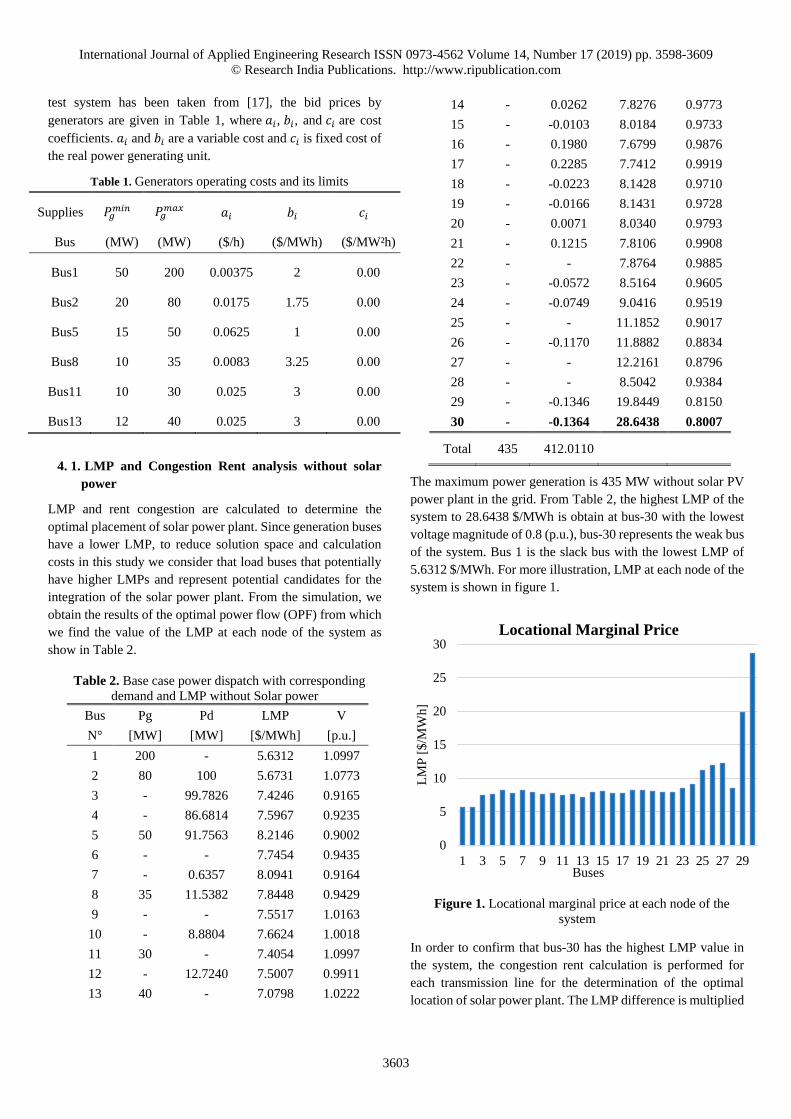
The maximum power generation is 435 MW without solar PV

power plant in the grid. From Table 2, the highest LMP of the

system to 28.6438 $/MWh is obtain at bus-30 with the lowest

voltage magnitude of 0.8 (p.u.), bus-30 represents the weak bus

of the system. Bus 1 is the slack bus with the lowest LMP of

5.6312 $/MWh. For more illustration, LMP at each node of the

system is shown in figure 1.

Figure 1. Locational marginal price at each node of the

system

In order to confirm that bus-30 has the highest LMP value in

the system, the congestion rent calculation is performed for

each transmission line for the determination of the optimal

location of solar power plant. The LMP difference is multiplied

0

5

10

15

20

25

30

1 3 5 7 9 11 13 15 17 19 21 23 25 27 29

LM

P [

$/M

Wh

]

Buses

Locational Marginal Price



3604

by the power transferred across the line, which gives the

congestion rent on this line for a base case as indicated in

equation (15). The line with the highest congestion rent

represents the congested transmission line and it represents the

optimal location of the solar power plant. Congestion rent

analysis is shown in Figure 2 as follows.

Figure 2. Congestion rent at each line of the system

From Figure 2 it is obtain that the line between bus-27 and bus-

30 has the highest congestion rent to 212.8856 $/h. we can see

that, this transmission line (from bus-27 to bus-30) is the most

congested line follows by line (from bus-1 to bus-3). Therefore,

by consider LMP analysis and congestion rent calculation, we

conclude that bus-30 with highest LMP value and highest rent

is the optimal placement of grid-tied solar PV system. Once the

optimal location of the solar power plant is determined, the

optimal sizing of the solar power plant is then performed using

Probability Density Function (PDF).

4. 2. Optimal sizing of grid-tied solar power

Solar power depends on meteorological conditions such as

irradiance, ambient temperature which are directly related to

geographical location [19]. For effective utilisation of PV

arrays the characteristics should be seriously analysed. For this

study, Sikasso region, which is located in Mali, is considered.

The study period of one year is divided into three seasons

Summer (March to June), Spring (July to October) and Winter

(November to February). Mean (µ) and standard deviation (σ)

of solar irradiance at each season are calculated from the

historical data [20] given in the appendix. The average value of

variation in solar irradiance in Sikasso is shown in the appendix.

It is observed that the irradiance is maximum in summer season.

For optimal sizing of solar power plant, Beta distribution

function based on Probability Density Function (PDF) is used

to model the solar panel. A matlab code is performed to

calculate the total output power in the three seasons of year by

using equations (16) to (25). Several solar panel with different

capacities and different specification are used to determine the

optimal solar panel that can get the necessary optimal output

power of solar for maximizing the social welfare and at the

same time reducing congestion in the transmission system.

Solar panels 220 W, 300W, 400 W and 500 W are used, their

specification parameters are given in [20], [24], [25] and show

in the appendix Table 2.

Matlab code calculate the total output power of solar power

plant during summer season, spring season and winter season

accordingly to the parameters of beta distribution function

(mean µ and standard deviation σ) of solar irradiance. Table 3

give the result of solar output power at different season and

with different capacity of solar panel.

Table 3 shows us that during summer season, solar irradiance

is maximal as the power of solar power is proportional to the

irradiance then the output power of solar power plant is also

maximal during that period. In winter, the power plant produces

the minimum of its capacity. At this level, we cannot say which

capacity of output power is the optimal power that can

maximize the social welfare and reduce the congestion.

0

50

100

150

200

Bu

s10

-Bus1

7B

us1

0-B

us2

0B

us1

0-B

us2

1B

us1

0-B

us2

1B

us1

0-B

us2

2B

us1

2-B

us1

4B

us1

2-B

us1

5B

us1

2-B

us1

6B

us1

3-B

us1

2B

us1

4-B

us1

5B

us1

5-B

us1

8B

us1

5-B

us2

3B

us1

6-B

us1

7B

us1

8-B

us1

9B

us1

-Bu

s3B

us2

0-B

us1

9B

us2

1-B

us2

2B

us2

2-B

us2

4B

us2

3-B

us2

4B

us2

4-B

us2

5B

us2

5-B

us2

6B

us2

5-B

us2

7B

us2

7-B

us2

8B

us2

7-B

us2

9B

us2

-Bu

s1B

us2

-Bu

s1B

us2

-Bu

s4B

us2

-Bu

s6B

us3

0-B

us2

7B

us3

0-B

us2

9B

us3

-Bu

s4B

us4

-Bus1

2B

us4

-Bu

s6B

us5

-Bu

s7B

us6

-Bus1

0B

us6

-Bus2

8B

us6

-Bu

s9B

us7

-Bu

s6B

us8

-Bus2

8B

us8

-Bu

s6B

us9

-Bus1

0B

us9

-Bus1

1

CR

[$

/h]

Transmission lines

Congestion Rent [$/h]



3605

Table 3. Solar output power capacities in MW

Solar panel

capacity Summer Spring Winter

220 W 87.716 72.810 66.063

300 W 120.54 99.913 90.598

400 W 151.23 131.03 114.54

500 W 198.83 164.98 149.67

To get the optimal size of solar power plant, the output powers

of PV obtain previously are integrated to the grid at bus-30 and

the OPF is performed for each output power of solar. The utility

of grid-tied solar PV is to reduce the gaps between supplies and

demands in the system, to reduce the losses and improve power

quality. In term of cost, solar power after installation has free

cost so that by introducing a solar power plant to the system the

cost of power paid by customer will be reduce, therefore the

social welfare will be maximized. Table 4 illustrates the cost of

power paid for each capacity of solar power and the total losses

of the system after connecting the solar power plant

corresponding.

Table 4. Cost of power paid by the customer after grid-tied

solar PV

Solar Output

Power [MW]

Pay

[$/h]

Total Losses

[MW]

66.063 196.669786 20.721

72.81 191.308307 20.185

87.716 180.548847 19.11

90.598 178.626551 18.919

99.913 172.774892 18.337

114.54 164.688911 17.531

120.54 161.606882 17.257

126.03 159.480786 17.143

131.03 158.096532 17.135

149.67 159.922223 17.911

151.23 160.706420 18.033

164.98 171.474949 19.525

198.83 233.158246 26.806

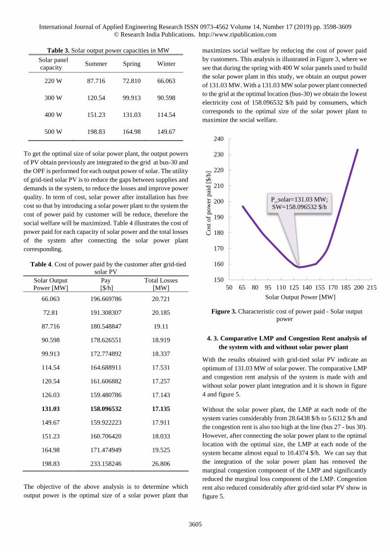
The objective of the above analysis is to determine which

output power is the optimal size of a solar power plant that

maximizes social welfare by reducing the cost of power paid

by customers. This analysis is illustrated in Figure 3, where we

see that during the spring with 400 W solar panels used to build

the solar power plant in this study, we obtain an output power

of 131.03 MW. With a 131.03 MW solar power plant connected

to the grid at the optimal location (bus-30) we obtain the lowest

electricity cost of 158.096532 $/h paid by consumers, which

corresponds to the optimal size of the solar power plant to

maximize the social welfare.

Figure 3. Characteristic cost of power paid - Solar output

power

4. 3. Comparative LMP and Congestion Rent analysis of

the system with and without solar power plant

With the results obtained with grid-tied solar PV indicate an

optimum of 131.03 MW of solar power. The comparative LMP

and congestion rent analysis of the system is made with and

without solar power plant integration and it is shown in figure

4 and figure 5.

Without the solar power plant, the LMP at each node of the

system varies considerably from 28.6438 $/h to 5.6312 $/h and

the congestion rent is also too high at the line (bus 27 - bus 30).

However, after connecting the solar power plant to the optimal

location with the optimal size, the LMP at each node of the

system became almost equal to 10.4374 $/h. We can say that

the integration of the solar power plant has removed the

marginal congestion component of the LMP and significantly

reduced the marginal loss component of the LMP. Congestion

rent also reduced considerably after grid-tied solar PV show in

figure 5.

P_solar=131.03 MW;

SW=158.096532 $/h

150

160

170

180

190

200

210

220

230

240

50 65 80 95 110 125 140 155 170 185 200 215

Co

st o

f p

ow

er p

aid

[$

/h]

Solar Output Power [MW]



3606

Figure 4. Comparison of LMP at each node of the system with and without solar power plant

Figure 5. Comparison of congestion rent with and without solar power plant

As solar power injects real power, its placement has a direct

effect of reducing LMP at the node where it is placed. The

location of solar power plant has an overall impact on the power

flow in the transmission system. The placement will therefore

influence the LMPs at nodes other than the node where it is

placed. Therefore, the penetration of solar power plant has a

positive influence on all nodes of the system. All customers

benefit from it based on the amount they receive. The need to

pay for the same amount of electricity is reduced compared to

the case without a solar PV plant.

In Table 5, a comparative review of social welfare with and

without solar power plant is illustrated. The results show that

0

5

10

15

20

25

30

1 2 3 4 5 6 7 8 9 10 11 12 13 14 15 16 17 18 19 20 21 22 23 24 25 26 27 28 29 30

LM

P [

$/M

Wh

]

Buses

LMP analysis with and without solar power plant

LMP [$/MWh] without solar power LMP [$/MWh] with solar power

0

50

100

150

200

Bus1

0-B

us1

7B

us1

0-B

us2

0B

us1

0-B

us2

1B

us1

0-B

us2

1B

us1

0-B

us2

2B

us1

2-B

us1

4B

us1

2-B

us1

5B

us1

2-B

us1

6B

us1

3-B

us1

2B

us1

4-B

us1

5B

us1

5-B

us1

8B

us1

5-B

us2

3B

us1

6-B

us1

7B

us1

8-B

us1

9B

us1

-Bu

s3B

us2

0-B

us1

9B

us2

1-B

us2

2B

us2

2-B

us2

4B

us2

3-B

us2

4B

us2

4-B

us2

5B

us2

5-B

us2

6B

us2

5-B

us2

7B

us2

7-B

us2

8B

us2

7-B

us2

9B

us2

-Bu

s1B

us2

-Bu

s1B

us2

-Bu

s4B

us2

-Bu

s6B

us3

0-B

us2

7B

us3

0-B

us2

9B

us3

-Bu

s4B

us4

-Bu

s12

Bus4

-Bu

s6B

us5

-Bu

s7B

us6

-Bu

s10

Bus6

-Bu

s28

Bus6

-Bu

s9B

us7

-Bu

s6B

us8

-Bu

s28

Bus8

-Bu

s6B

us9

-Bu

s10

Bus9

-Bu

s11

CR

[$

/h]

Transmission lines

Congestion Rente analysis with and without solar power plant

CR [$/h] without solar power CR [$/h] with solar power



3607

in addition to reducing the LMP at the level of all buses in the

system, there is a considerable maximization of social welfare

by reducing the cost of power paid by customer and the

problem of congestion on transport lines is reduced

considerably.

Table 5. Social Welfare analysis

Output Parameters Output (MW) Output (MW)

Without Solar With Solar

Total losses 37 .361 17 .143

Bid losses 22 .476 -17 .888

Total transaction level 705.068041 746.28761

IMO PAY ($/h) 1215.42159 159.480786

VI. CONCLUSION

The purpose of the research was to assess the impact of

renewable energy resources mainly solar power on

transmission congestion management in the deregulated power

system and the maximization of social welfare using LMP

analysis. LMP, which consists of a congestion component, as

well as a fixed component and a loss component, plays an

important role in the deregulated power market. It is used in a

practical way for optimal placement of solar power plant in this

study and congestion rent is used to confirm the effectiveness

of the Highest LMP Method. Therefore, the measures

necessary to maintain the lowest possible LMP values are a

priority. The MATLAB-PSAT software's Optimal Power Flow

(OPF) method is used and the LMP at each bus is determined

by maximizing social welfare. The optimal sizing and location

of solar power plant is formulated from the perspective of

maximizing social welfare. System locations are examined to

study the impact of renewable energy resources penetration on

LMPs, so it is concluded that:

• Locally, solar energy has the effect of eliminating the

marginal congestion component of the LMP, so making the

LMP equal to each node of the system.

• The optimal dispatch from solar power is thus found to

reduce the congestion rent and shadow prices associated with

the line flow.

• Moreover, solar power with free cost is found to have better

performance in terms of alleviating congestion in the network

and maximising social welfare.

V. REFERENCES

[1] H. Ahmadi, M. Khanabadi, and H. Ghasemi,

“Transmission system reconfiguration for congestion

management ensuring transient and voltage stability,”

2013 13th Int. Conf. Environ. Electr. Eng. EEEIC 2013 - Conf. Proc., pp. 22–26, 2013.

[2] M. Khanabadi, M. Doostizadeh, A. Esmaeilian, and M.

Mohseninezhad, “Transmission congestion

management through optimal distributed generation’s

sizing and placement,” 2011 10th Int. Conf. Environ. Electr. Eng. EEEIC.EU 2011 - Conf. Proc., pp. 0–3,

2011.

[3] A. Swami, “Transmission Congestion Impacts on

Electricity Market: An Overview,” Int. J. Emerg. Technol. Adv. Eng., vol. 3, no. 8, 2013.

[4] A. Abirami and T. R. Manikandan, “Locational

Marginal Pricing Approach for a Deregulated

Electricity Market,” Int. Res. J. Eng. Technol., vol. 2,

no. 9, 2015.

[5] H. Ahmadi and H. Lesani, “Transmission congestion

management through lmp difference minimization: A

renewable energy placement case study,” Arab. J. Sci. Eng., vol. 39, no. 3, pp. 1963–1969, 2013.

[6] K. Singh, V. K. Yadav, N. P. Padhy, and J. Sharma,

“Congestion management considering optimal

placement of distributed generator in deregulated

power system networks,” Electr. Power Components Syst., vol. 42, no. 1, pp. 13–22, 2014.

[7] M. N. Rothbard, “Power & Market,” vol. 1, no. 3, pp.

421–426, 100AD.

[8] K. B. R. Kumar and S. C. Mohan, “LMP Congestion

Management Using Enhanced STF-LODF in

Deregulated Power System,” Sci. Res. Publ., no. 7, pp.

2489–2498, 2016.

[9] B. Liu, J. Kang, N. Jiang, and Y. Jing, “Cost Control of

the Transmission Congestion Management in

Electricity Systems Based on Ant Colony Algorithm,”

Energy Power Eng., no. 3, pp. 17–23, 2011.

[10] H. Patel and R. Paliwal, “Congestion Management in

Deregulated Power System using FACTS Devices,”

vol. 8, no. 2, pp. 175–184, 2015.

[11] M. Sarwar and A. S. Siddiqui, “Congestion

Management in Deregulated Electricity Market Using

Distributed Generation,” IEEE INDICON 2015, pp. 1–

5, 2015.

[12] Kankar Bhattacharya, M. H. J. Bollen, and J. E.

Daalder, Operation of Restructured Power Systems,

vol. 39, no. 5. 2001.

[13] M. Afkousi-Paqaleh, A. Abbaspour-Tehrani Fard, and

M. Rashidinejad, “Distributed generation placement

for congestion management considering economic and

financial issues,” Electr. Eng., vol. 92, no. 6, pp. 193–

201, 2010.



3608

[14] D. Gautam and M. Nadarajah, “Influence of distributed

generation on congestion and LMP in competitive

electricity market,” Int. J. Electr. Comput. Energ. Electron. Commun. Eng., vol. 4, no. 3, pp. 822–829,

2010.

[15] S. Padmini and B. Sahoo, “Analysis of LMP in a

Competitive Electricity Market,” Int. J. Pure Appl. Math., vol. 118, no. 24, pp. 1–7, 2018.

[16] I. Leevongwat, P. Rastgoufard, and E. J. Kaminsky,

“Status of deregulation and locational marginal pricing

in power markets,” Proc. Annu. Southeast. Symp. Syst. Theory, no. 3, pp. 193–197, 2008.

[17] N. C. Abdullah Urkmez, “DETERMINING SPOT

PRICE AND ECONOMIC DISPATCH,” vol. 15, no.

1, pp. 25–33, 2010.

[18] M. Shahidehpour, H. Yamin, and Z. Li, Market Operations in Electric Power Systems: Forecasting, Scheduling and Risk Management. 2002.

[19] P. Kayal and C. K. Chanda, “Optimal mix of solar and

wind distributed generations considering performance

improvement of electrical distribution network,”

Renew. Energy, vol. 75, pp. 173–186, 2015.

[20] V. Suresh and S. Sreejith, “Economic Dispatch and

Cost Analysis on a Power System Network

Interconnected With Solar Farm,” Int. J. Renew. Energy Rsearch, vol. 5, no. 4, 2015.

[21] V. Suresh and S. Sreejith, “Reserve Constrained

Economic Dispatch Incorporating Solar Farm using

Particle Swarm Optimization,” vol. 6, no. 1, 2016.

[22] P. Sebah and X. Gourdon, “Introduction to the Gamma

Function,” vol. 0, no. 1, pp. 1–20, 2002.

[23] D. Gautam and N. Mithulananthan, “Optimal DG

placement in deregulated electricity market,” Electr. Power Syst. Res., vol. 77, no. 12, pp. 1627–1636, 2007.

[24] A. Resistance, “300 W – 320 W Poly-crystalline Solar

Module,” www.sunceco.com. .

[25] K. M. Bs and E. N. Photovoltaic, “LG400N2W-V5 I

LG395N2W-V5 400w / 395w,” 2016. .

[26] “Longitude, latitude, GPS coordinates of Mali,”

www.gps-longitude-latitude.net/coordonnees-gps-de-mali. .

VI. APPENDICES



3609

Figure A.1. IEEE 30-Bus System

Table A.1. Specifications of 220 W, 300 W, 400 W and 500 W solar panel [20], [24], [25]

Parameter 220 W 300 W 400W 500 W

Maximum Power Point Voltage, VMPPT [V] 28.36 37.23 40.6 48.63

Maximum Power Point Current, IMPPT [A] 7.76 8.06 9.86 10.28

Open Circuit Voltage, VOC [V] 36.96 44.71 49.3 58.95

Short Circuit Current, ISC [A] 8.38 8.947 10.47 10.87

Nominal Operating Temperature, NOT [°C] 43 47 44 45

Ambient Temperature, TA [°C] 30.76 30.76 30.76 30.76

Voltage Temperature Coefficient, Kv [V/°C] -0.1278 -0.1520 -0.1282 -0.1945

Current Temperature Coefficient, Ki [A/°C] 0.00545 0.004473 0.002094 0.006304

Total number of PV modules 350 000 350 000 350 000 350 000

Table A.2. Beta Distribution Function for Solar Irradiance

Modeling [20]

Parameter Summer Spring Winter

Mean (µ) 0.9302 0.7834 0.7152

Standard

Deviation (𝜎) 0.1088 0.1772 0.2402

Figure A.2. Monthly variation of solar irradiation (KW/m2)

in Sikasso region of Mali (17° 34' 14.491" N 3° 59' 46.198"

W) [26]

0

0.05

0.1

0.15

0.2

0.25

0.3

0.35

0.4

0.45

Irradiances [KW/m2]

optimal sizing of grid tied solar pv for transmission ... · congested power systems using facts...

Documents