optimal scheduling of demand side flexible units under
TRANSCRIPT
Optimal scheduling of demand side flexible units under uncertainty in
SmartGrids
Stig Ødegaard Ottesen
Presentation outline
• Intro – SmartGrids and flexibility • Optimization model • Case study • Future research

SmartGrid intro • Active interaction between smart prosumers
and energy system/market to create benefits in the value chain
• Demand side technologies
• Pricing regimes, business models
• Demand side flexibility

Increasing need for demand side flexibility
• Integration of renewable generation • Intermittent • Non dispatchable • Difficult to predict
• Integration of electrical vehicles
• In general more dynamics in the distribution grid
• This flexibility exists at distribution level

Our problem • Smart prosumer (building with flexible energy resources
(loads, generation/conversion, storage)) • El-prices that vary as a function of time and/or volume • Participation in the end-user market
• How to decide a short term (day ahead) optimal schedule
for the flexible resources? • Need a general model that minimizes total costs with
respect to – Technical, comfort and economical constraints – All information is not known at the decision point
5
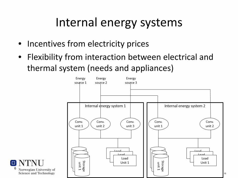
Internal energy systems • Incentives from electricity prices • Flexibility from interaction between electrical and
thermal system (needs and appliances)
6
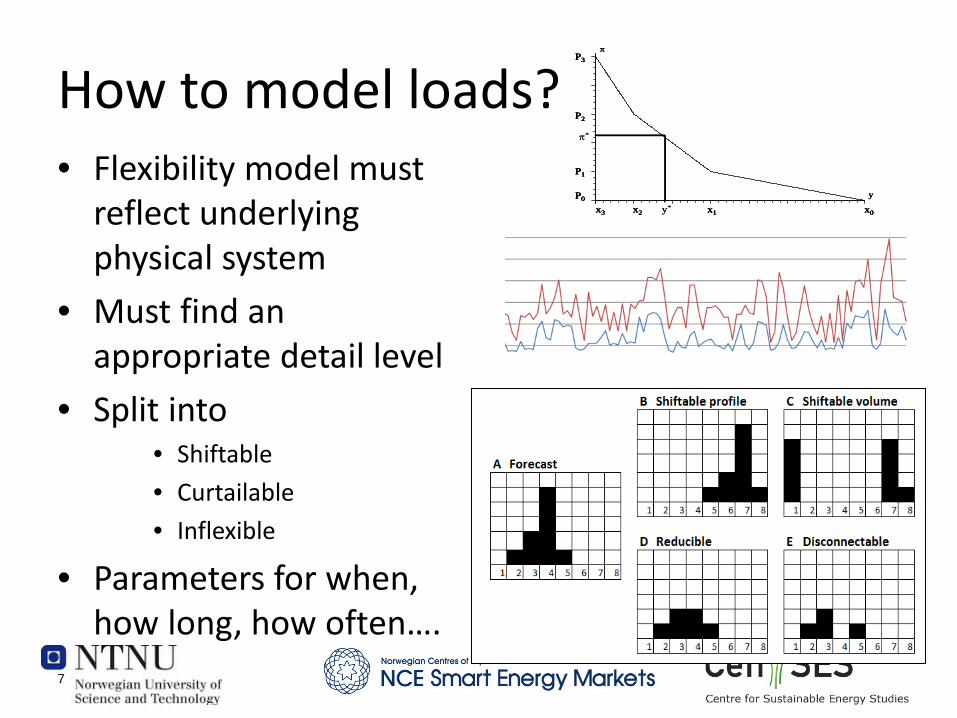
How to model loads? • Flexibility model must
reflect underlying physical system
• Must find an appropriate detail level
• Split into • Shiftable • Curtailable • Inflexible
• Parameters for when, how long, how often….
7
P0
P1
P2
P3
x0x1x2x3
π
y
y*
π*
P0
P1
P2
P3
x0x1x2x3
π
yP0
P1
P2
P3
x0x1x2x3
P0
P1
P2
P3
x0x1x2x3
π
y
y*
π*

Optimization model
• Objective: Minimize expected total costs
• Subject to:
– Energy carrier constraints – Converter constraints – Storage constraints – Load constraints – Energy system balances
• Stochastisk mixed integer problem (SMIP)
8
, , , , , , , , ,
, , , , , , ,
minC
energy net in cap cap start startupa t s a t s a a s o y t s y o
a A t T a A y Y o O t Ts sales net out
s S d y d y t s a t a t sy Y t T a A t Td D
P P Gz R
X P
χ χ α
ϕ χ
−
∈ ∈ ∈ ∈ ∈ ∈
−∈
∈ ∈ ∈ ∈∈
+ + +
= ⋅ −
∑∑ ∑ ∑∑∑∑ ∑ ∑∑ ∑∑

Case-study
• Matematical model defined and implemented in Xpress
• Case-study performed based on university college building in Halden – in close cooperation with Statsbygg
9

Energy system model • Flexible loads:
– Shiftable volume • Swin area: whole day • Room: 2 and 2 hours
– Shiftable profile • Snow melting (4 hours)
– Curtailable • Lights. 20% dimmed
• Heat storage: • 37 kWh, maks 10 kW
• Energy carrier substitution: • Can change any time • Must run for minimum 4 hours when
started • Small startup-cost

Load forecasting model • At decision time load is not known - need a load
forecast • Model based on multiple linear regression with
exogenous explanatory variables • Load can be explained by hour of the day, whether
workday or not, out-door temperature and month
11
24 24 24
, , ,1 1 1
24 12
, ,1 1
workday hour workday workday hour workday nonworkday hour nonworkdayt h t h t h t h t t h t h t
h h h
nonworkday hour nonworkday monthh t h t t m t m t
h m
L D D D D D D
D D D t T
µ α β τ α
β τ γ ε
= = =
= =
= + + + +
+ + ∀ ∈
∑ ∑ ∑
∑ ∑
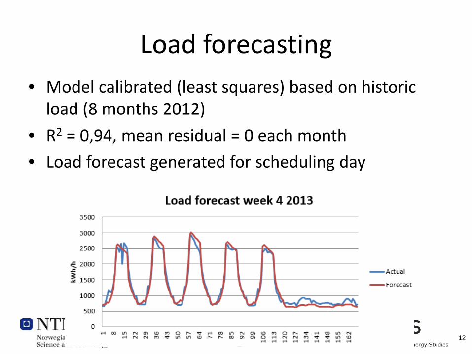
Load forecasting • Model calibrated (least squares) based on historic
load (8 months 2012) • R2 = 0,94, mean residual = 0 each month • Load forecast generated for scheduling day
12
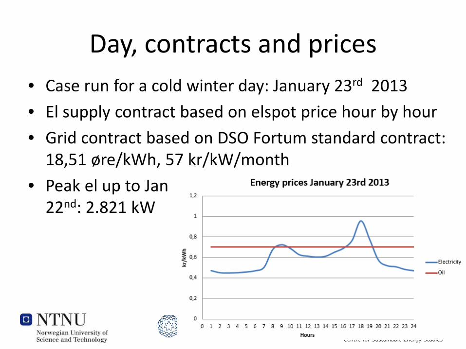
Day, contracts and prices • Case run for a cold winter day: January 23rd 2013 • El supply contract based on elspot price hour by hour • Grid contract based on DSO Fortum standard contract:
18,51 øre/kWh, 57 kr/kW/month • Peak el up to Jan
22nd: 2.821 kW

Case study main results • Target: Decide schedule for all flexible units (el/oil converter,
storage, shiftable/curtailable load units) • Flexibility used to
exploit: – El-price variations
during the day – Price variations
between el and oil – To reduce peak
electricity
• Net cost saving compared to no flexibility: – 1.000 kr energy – 11.000 kr peak
14
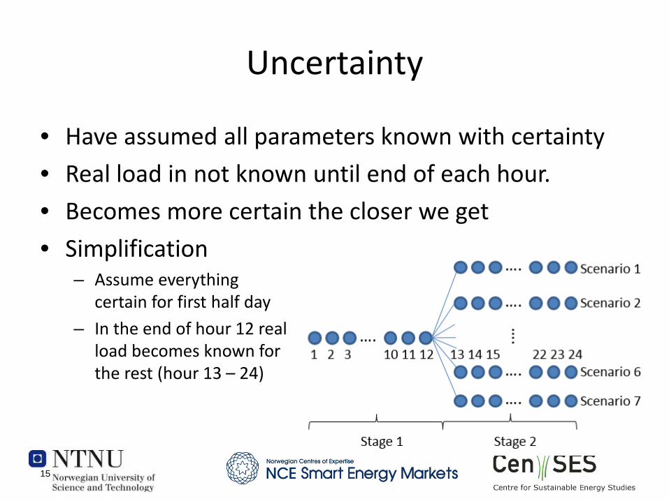
Uncertainty
• Have assumed all parameters known with certainty • Real load in not known until end of each hour. • Becomes more certain the closer we get • Simplification
– Assume everything certain for first half day
– In the end of hour 12 real load becomes known for the rest (hour 13 – 24)
15

Scenario generation • 7 load scenarios based on load forecast for actual
day + sampled residuals • Residuals strongly
auto correlated – sample day randomly and take whole series (hour 13 – 24)
• Repeat until mean residual ≈ 0
16
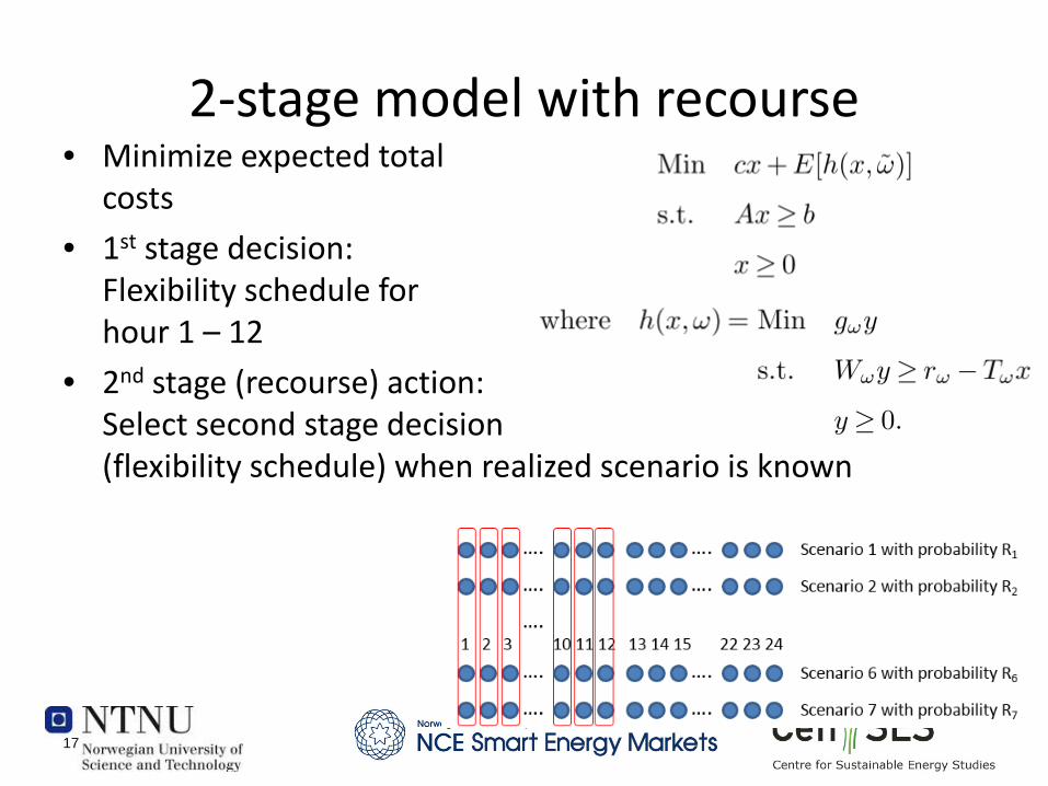
2-stage model with recourse • Minimize expected total
costs • 1st stage decision:
Flexibility schedule for hour 1 – 12
• 2nd stage (recourse) action: Select second stage decision (flexibility schedule) when realized scenario is known
17
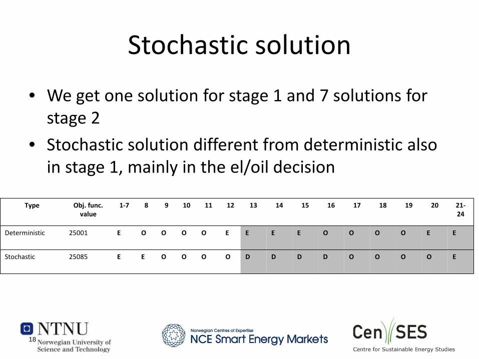
Stochastic solution
• We get one solution for stage 1 and 7 solutions for stage 2
• Stochastic solution different from deterministic also in stage 1, mainly in the el/oil decision
18
Type Obj. func. value
1-7 8 9 10 11 12 13 14 15 16 17 18 19 20 21-24
Deterministic 25001 E O O O O E E E E O O O O E E
Stochastic 25085 E E O O O O D D D D O O O O E
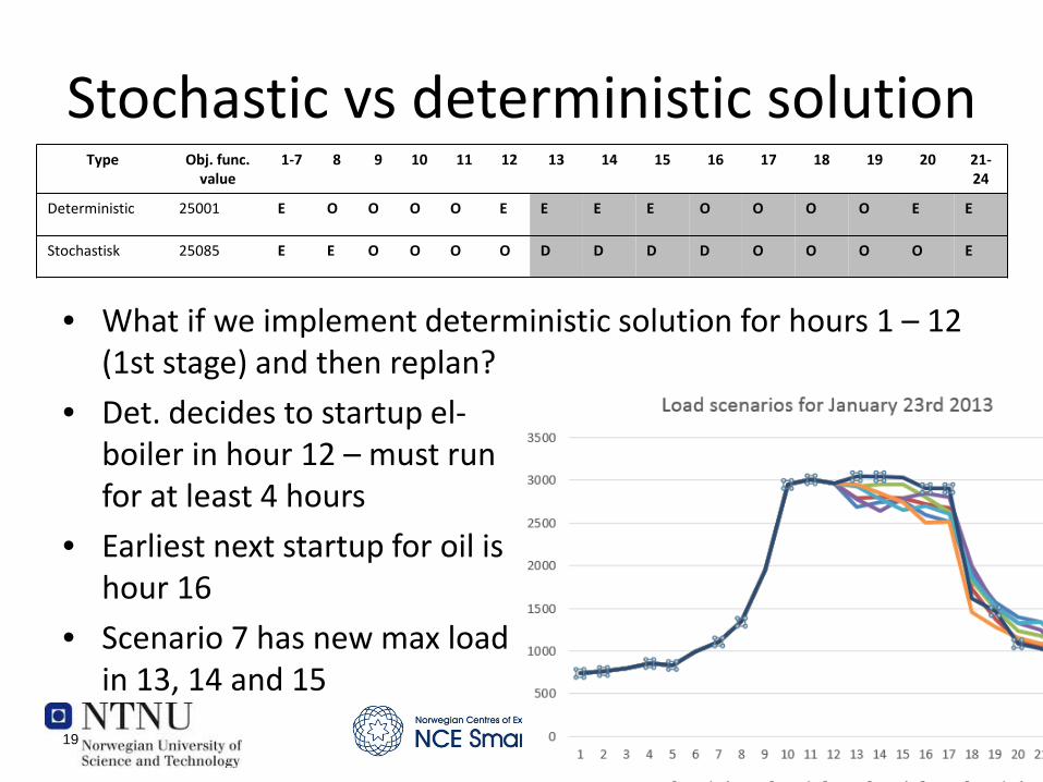
Stochastic vs deterministic solution
• What if we implement deterministic solution for hours 1 – 12
(1st stage) and then replan? • Det. decides to startup el-
boiler in hour 12 – must run for at least 4 hours
• Earliest next startup for oil is hour 16
• Scenario 7 has new max load in 13, 14 and 15 19
Type Obj. func. value
1-7 8 9 10 11 12 13 14 15 16 17 18 19 20 21-24
Deterministic 25001 E O O O O E E E E O O O O E E
Stochastisk 25085 E E O O O O D D D D O O O O E
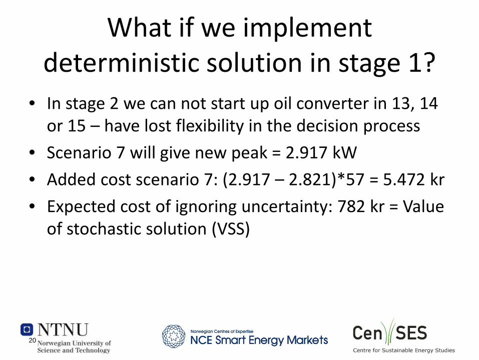
What if we implement deterministic solution in stage 1?
• In stage 2 we can not start up oil converter in 13, 14 or 15 – have lost flexibility in the decision process
• Scenario 7 will give new peak = 2.917 kW • Added cost scenario 7: (2.917 – 2.821)*57 = 5.472 kr • Expected cost of ignoring uncertainty: 782 kr = Value
of stochastic solution (VSS)
20

Discussion • Concept model described • Quantification of real cost reduction potential:
– Flexibility parameters must be properly estimated – Run model over larger period – Rolling planning horizon – What happens in real life (none of the scenarios realize) – Rather simplified stage model and scenario generation method
• Selected one single day, high load (monthly peak) and large price variations
• Current incentives in Norway weak – stronger in other countries
• Type of contract crucial
21
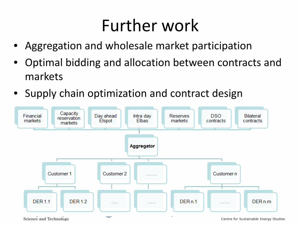
Further work • Aggregation and wholesale market participation • Optimal bidding and allocation between contracts and
markets • Supply chain optimization and contract design
22

Thank you for your attention
Stig Ødegaard Ottesen Research scientist, PhD candidate,
NCE Smart Energy Markets, NTNU, Department of industrial economics
and technology management +47 90973124