optimal placement of reactive power supports for loss minimization
TRANSCRIPT

u.mai
Optimal Placement of Reactive Power Supports for
Loss Minimization: The Case of A Georgian
Regional Power Grid
Thesis for the Degree of Master of Science
Otar Gavasheli
Division of Electric Power Engineering
Department of Energy and Environment
CHALMERS UNIVERSITY OF TECHNOLOGY
Göteborg, Sweden, November 2007

2 | P a g e

3 | P a g e
Optimal Placement of Reactive Power Supports for
Loss Minimization: The Case of A Georgian
Regional Power Grid
Otar Gavasheli
Division of Electric Power Engineering
Department of Energy and Environment
CHALMERS UNIVERSITY OF TECHNOLOGY
Göteborg, Sweden, November 2007

4 | P a g e
Optimal Placement of Reactive Power Supports for Loss Minimization: The Case of A Georgian
Regional Power Grid
Otar Gavasheli
© Otar Gavasheli, November 2007.
Division of Electric Power Engineering
Department of Energy and Environment
CHALMERS UNIVERSITY OF TECHNOLOGY 412 96 Göteborg
Sweden
Cover page courtesy of ABB Power Capacitors

5 | P a g e

6 | P a g e

7 | P a g e
Abstract
Power system operators/planners are always faced with the problem of how to minimize
the transmission loss. There are a number of ways to achieve this goal. In this thesis, new
methods for optimal capacitor placement for transmission loss minimization are proposed.
Proposed methods are based on the optimal power flow formulations, which enable the cost-
benefit analysis and multi-objective optimization assessment of reactive power support
investment. For better illustration of proposed methods, they are applied to a real and test
transmission networks.
In the cost-benefit analysis, reactive power supports are applied to the power system for
transmission loss minimization. The candidate places for reactive power support allocation
are defined in advance according to where the highest reactive power flow is observed. The
benefits after application of reactive power supports are calculated. Benefits considered are
the benefits from recovered transmission losses due to the reactive power addition. The
benefits are then compared with investments, which would be required for the addition of
reactive power supports and in this way the economical justification in reactive power
support addition can be made. This method is applied to the real transmission network of a
Georgian regional grid. After analyzing the obtained results, we can observe that in some
cases even though the losses are minimized up to the minimal level, economically it is not
optimal since in such cases, high investment costs are involved. The optimal cases are those
where the losses are a bit higher than possible minimum and the investments are minimal
also compared to what is required for achieving of minimal transmission losses. Only these
optimal cases can justify the investments, made for loss minimization. In the multi-objective
optimization several objective functions are proposed in one overall objective function. The
optimized functions are minimization of total investment in reactive power support, average
voltage deviation, minimization of total system loss and total system cost. At the beginning,
optimum values for each objective function is found one by one separately and these optimal
values are included while solving for overall objective function. During optimization of all
these objectives within one overall objective, we have opportunity to optimize each objective
according to what is our interest in it compared to other optimized objectives. This is done
using the priority order multipliers, which has each of the objective functions. CIGRE 32 bus
test system is used for illustration of this method. Three cases with different values of priority
order multipliers are solved and discussed. In the obtained results we can observe how the
values of optimized objective functions are changed to reflect their priority orders assigned in
the overall objective function.
Key words: Loss minimization, reactive power support, optimal power flow, cost-
benefit analysis, multi-objective optimization.

8 | P a g e

9 | P a g e
Acknowledgement
First of all I would like to thank my supervisor, Dr. Tuan A. Le for his invaluable support
and regular reviewing of my progress and competent advices despite his very busy schedule.
Also I would like to thank him for all the knowledge, which I received from his lectures and
personal consultations.
I would like to thank Swedish Institute and Sida for the MKP scholarship, which I was
receiving from them during all my study period in Sweden.
I gratefully acknowledge the staff of the technical department of Energo-Pro Georgia,
especially Mr. Mamuka Papuashvili, the head of the department, for their great supports,
insights and discussions while I was carrying out the work in Georgia.

10 | P a g e

11 | P a g e
Table of Contents
Chapter 1 ........................................................................................................................ 13
Introduction ........................................................................................................... 13
1.1. Technical losses ......................................................................................... 13
1.2. Proposed methods ...................................................................................... 14
1.3. Scope of the thesis work ............................................................................ 14
1.4. Thesis overview ......................................................................................... 15
Chapter 2 ........................................................................................................................ 17
Literature Review .................................................................................................. 17
2.1. Optimal Power Flow .................................................................................. 17
2.2. CYME and GAMS Softwares used for OPF modeling and simulations ...... 18
2.3. Technical losses in power systems ............................................................. 19
2.4. Reactive power compensation .................................................................... 20
2.3. Shunt capacitors and their types ................................................................. 22
2.4. Methods for optimal capacitor placement ................................................... 23
Chapter 3 ........................................................................................................................ 31
Methodology ......................................................................................................... 31
3.1. Method applied to Georgian regional grid .................................................. 31
3.2. Method with multi objective function applied to CIGRE 32 bus system ..... 32
Chapter 4 ........................................................................................................................ 35
Simulations with Real Networks ............................................................................ 35
4.1. Simulations with Georgian regional grid .................................................... 35
4.1.1. Description of investigated Georgian regional grid .................................... 35
4.1.2. Power system modeling and simulation for Georgian regional grid ........... 39
4.1.3. Simulation results and their analysis for Georgian regional grid ............... 42
4.2. Simulations with CIGRE 32 bus test system ............................................... 45
4.2.1. Description of CIGRE 32 bus test system ................................................... 45
4.2.2. Power system modeling and simulations for CIGRE 32 bus system ............ 46
4.2.3. Simulation results and their analysis for CIGRE 32 bus system .................. 47
Chapter 5 ........................................................................................................................ 61
Conclusions ........................................................................................................... 61
Chapter 6 ........................................................................................................................ 63
Future work ........................................................................................................... 63
Appendix A ........................................................................................................... 67
Optimal Placement of Reactive Power Supports for Transmission Loss
Minimization: The Case of Georgian Regional Power Grid, Otar Gavasheli and Le
Anh Tuan............................................................................................................... 67

12 | P a g e

13 | P a g e
Chapter 1 Introduction
In this chapter the general overview of thesis and its topic-power losses are discussed. The
ways for reduction of power losses will be reviewed here. Solution methods, which will be
used for solving of the problems, will be discussed and the content of the thesis will be
presented, as well as the publication from this thesis.
1.1. Technical losses
Technical losses are inescapable physical phenomenon occurring during the transfer of
energy from generating plants to load centers. During this transfer process some of the input
energy is dissipated in conductors and transformers along the delivery route. Losses occur in
all conductors, and may be any of three types: copper, dielectric and induction radiation
losses. The main portion of total transmission losses consists of copper losses. Copper losses
are the I2R losses that are inherent in all conductors because of the finite resistance of the
conductors. These losses are due to the current flowing in the electrical network. In AC
systems the copper losses are higher due to skin effect.
Technical losses can be calculated based on the natural properties of components in the
power system: resistance, reactance, capacitance, voltage, current, and power, which are
routinely calculated by utility companies as a way to specify what components will be added
to the systems, in order to reduce losses and improve the voltage levels.
Transmission losses in the network constitute economic loss providing no benefits.
Transmission losses are construed as a loss of revenue by the utility. The magnitude of each
of these losses needs to the accurately estimated and practical steps taken to minimize them.
From the utility perspective, transmission losses need to be reduced to their optimal level.
In a typical system, network losses are in range of 5 to 10% of the total power system,
which would cost millions of dollars every year [1]. Therefore, loss minimization is one of
the important objectives in operating the transmission networks. It is even more so in the
context of deregulated power system, since fair allocation of the network losses has very
important impact on all users. This is because unfair allocation causes cross subsidies and it
gives wrong indicative signals to the network operator and users. A user who causes more

14 | P a g e
network losses must be charged more while a user who helps to reduce the losses, due to
counter flow, must be rewarded.
One commonly used way for transmission loss reduction and improving voltage levels in
power systems is addition of reactive power supports to where it is necessary. Reactive
power addition can be beneficial only in case if it is correctly applied. Correct application
means choosing the correct position and size of reactive power support. Different types of
reactive power supports can be applied, but for our case we will use widespread reactive
power support type-shunt capacitors.
1.2. Proposed methods
In this thesis, two methods to evaluate the optimal placement of reactive power supports
are proposed.
One method is based on the cost-benefit analysis. The costs are economic costs, which
include direct and indirect costs. The direct cost of reactive power sources are investment and
operating costs. The indirect cost would include the opportunity cost of generators which
reduce real power production for reactive power production. The benefits from reactive
power supports are defined as the reduced generation costs due to reduced losses as well as
other quantifiable benefits of reduced total system cost. The dispatch costs could be reduced
due to the fact that power generation schedules can be changed by increased transmission
capability in the network which will allow for more generation from cheap sources to be
delivered to the load centers. The benefits can also stem from the fact that more energy can
be sold to the customers which will increase the sales (and profits) due to higher transmission
capacity.
Another proposed method optimizes several objective functions at the same time within
one general objective. The optimized objectives are minimization of total investment in
reactive power support, average voltage deviation, minimization of total system loss and total
system cost. These objective functions are one of the most important objectives for every
transmission and distribution systems.
1.3. Scope of the thesis work
The scope of work of this thesis work includes developing of methods for correct reactive
power allocation in power systems with the objective function of loss minimization. The
multi-objective optimization is also included. The modeling of Georgian regional grid and
further simulations using newly developed method for loss minimization will be done in
CYME [10] power engineering software. Also another model of CIGRE 32 bus system [23]
will be made in GAMS software [22], where we will implement our method with multi-
objective optimization. The obtained results will be discussed and analyzed.

15 | P a g e
1.4. Thesis overview
This thesis consists of six chapters. In chapter 2 the literature review about technical
losses is given. Also the discussion about this work is included. In chapter 3 the chosen
methodologies for solving the problem are discussed. In chapter 4 applications of our
discussed theories to the real network and test system will be shown. In the same chapter the
review of the simulated Georgian regional grid and CIGRE 32 bus test system together with
simulation results are given. In chapter 5 the conclusions are made and in chapter 6 the future
work is discussed.
In appendix A the publication from our thesis can be found. Publication includes the
method with cost-benefit analysis that was applied to the Georgian regional grid.
Methodology description and results of application of the method to the real power system as
well as analysis of the obtained results are included also in this publication.

16 | P a g e

17 | P a g e
Chapter 2 Literature
Review In this thesis we are studying the technical losses reduction method-optimal allocation of
reactive power in electrical power systems as well as the way of optimization of several
objective functions at the same time. Both these methods we are implemented based on
Optimal Power Flow framework. Accordingly the logical first step is to understand what
Optimal Power Flow is and complete picture of power systems technical losses. What is
reactive power and why the reactive power allocation could help in reducing of losses. In
this chapter the basic idea of Optimal Power Flow will be presented. Technical losses as well
as reactive power compensation as loss reduction method will be presented. The general
types of shunt capacitors and ways for optimal capacitor placement will be reviewed. Also
some interesting papers about loss minimization and optimal reactive support allocation will
be discussed.
2.1. Optimal Power Flow
Optimal Power Flow (OPF) was first introduced in early 1960s as an extension of the
conventional Economic Load Dispatch problem to determine optimal settings for control
variables while satisfying different constraints.
In practice power flow in power system follows the Kirchoff’s Laws, which are commonly
known as a load flow equations. When these load flow equations are introduced in economic
load dispatch as demand-supply balance constraints, the optimum solution is obtained, where
the set of decision variables are satisfying the physical laws of electricity while the pre-
defined objective function is optimized. Objective function can be loss minimization, cost
minimization etc. This kind of problem formulation is called Optimal Power Flow (OPF),
which is a static, constrained, nonlinear optimization problem.
The main equations used in OPF are the active and reactive power demand-supply balance
equations, which are obtained from basic Kirchoff’s Laws:
18 | P a g e
Where V is bus voltage, δ is the angle associated with V, Yi,j is the element of bus
admittance matrix, θ is the angle associated with Yi,j, P and Q are the active and reactive
power generations respectively, PD and QD are the active and reactive power consumptions
respectively.
Beside of these basic equations, we also have active and reactive power generation limits
as follows:
Here PMin
and PMax
Stand for lower and upper limits for active power generation and QMin
and QMax
are for lower and upper limits of reactive power generation.
For voltages we have limitations also:
Where VMin
and VMax
are minimal acceptable voltage levels at each bus.
2.2. CYME and GAMS Softwares used for OPF modeling and
simulations
In this thesis for modeling of power systems and simulations we use CYME and GAMS
simulation softwares. Brief description of these softwares is given here.
Modeling of Georgian regional grid was done in PSAF part of CYME software systems.
PSAF is the same as Power System Analysis Framework. Optimal Power Flow analysis
module of PSAF, which we used for our simulations, gives us possibility to make advanced
system planning studies to optimize system performance, examine cost-efficient operational
planning alternatives, define system control strategies and optimize equipment utilization. As
a result we get better overall system management possibility.
OPF module of FSAF software relies on robust barrier-method based on nonlinear
optimization techniques that permit fully coupled optimization, with the entire set of system
control variables, including generation schedules, transformer taps, phase shifter settings, etc.

19 | P a g e
PSAF OPF module gives us possibility to include various constrains in model. Constrains
can be bus voltage magnitude limits, branch flow limits (MW, MVAR, MVA, Amps),
generator reactive power limits, generator active power limits, Transformer tap changer
limits etc.
PSAF OPF module also gives us opportunity to optimize different objective functions at
the same time, while strictly respecting system constraints. System controls are automatically
adjusted to provide least cost design or an operational mix.
The optimal solution insures that system losses, generation costs, Reactive Power support
requirements and different objectives are simultaneously optimized.
For implementation of method with multi objective function we use GAMS software. The
General Algebraic Modeling System (GAMS) is high-level modeling software for
mathematical programming and optimization. Modeling futures of GAMS software includes
possibility of modeling of linear, nonlinear and mixed integer optimization problems. The
software is designed for complex, large scale modeling applications, and allows the user to
build large maintainable models. The system contains a group of integrated solvers, such are
LP (Linear Programming), NLP (Non Linear Programming), MINLP (Mixed Integer Non
Linear Programming) and other solvers.
In our case CIGRE 32 bus test system was modeled in GAMS. We are using NLP solver
for solving of our multi objective function.
2.3. Technical losses in power systems
Technical losses are naturally occurring losses (caused by actions internal to the power
system) and consist mainly of power dissipation in electrical system components such as
transmission lines, power transformers, measurement systems, etc. due to their internal
electrical resistance. If we express the transmission losses in term of bus voltages and
associated angles, then the losses can be expressed with equation (2.1) [l3]:
Where Gi,j is the conductance of the line i-j, Vi and Vj are line voltages and δi and δj the
line angles at the line i and j ends respectively.
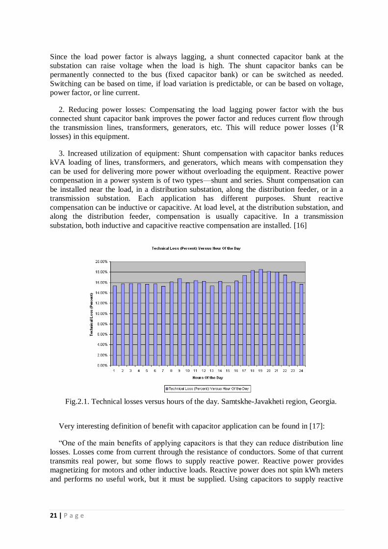
It is not possible to achieve zero losses in a power system, but it is possible to keep them
at minimum. From figure 2.1, taken from [9] which belongs to our investigated Georgian
regional grid, we can observe, that losses are becoming higher when the system is heavily
loaded and transmission lines are transmitting high amount of power. The transmitted power
for this case consists of active and reactive power. Necessity of reactive power supply
together with active power is one of the disadvantages of the power generation, transmission
and distribution with alternating current (AC). Reactive power can be leading or lagging. It is
either generated or consumed in almost every component of the power system. In AC system

20 | P a g e
each component’s impedance consists of two components, resistance and reactance.
Reactance can be either inductive or capacitive, which contribute to reactive power in the
circuit. In general most of the loads are inductive and they should be supplied with lagging
reactive power.
2.4. Reactive power compensation
We need to release the power flow in transmission lines for partially solving of problem of
losses as well as other problems. We can’t do anything with active power flow, but we could
supply the reactive power locally where it is highly consumed in a system. In this way the
loading of lines would decrease. It would decrease the losses also and with this action the
problem of voltage drops could be solved also. By means of reactive power compensation
transmission system losses can be reduced as shown in many papers in the literature, see e.g.,
[2]-[4]. It has also been widely known that the maximum power transfer of the transmission
system can be increased by shunt reactive power compensation, typically by capacitors banks
placed at the end of the transmission lines or a the load terminals [5]. Therefore, planning of
reactive power supports would give benefits to the users of the transmission systems, in
terms of loss reduction, among other technical benefits, such as improving steady-state and
dynamic stability, improve system voltage profiles, etc. which are documented in [6]. The
reactive power planning problem involves optimal allocation and sizing of reactive power
sources at load centers to improve the system voltage profile and reduce losses. However,
cost considerations generally limit the extent to which this can be applied.
―The book Edited by T. J. E. Miller contains perfect summary of why we must use
reactive compensation: ―…the transmission of active power requires a difference in angular
phase between voltages at the sending and receiving points (which is feasible within wide
limits), whereas the transmission of reactive power requires a difference in magnitude of
these same voltages (which is feasible only within very narrow limits). But why should we
want to transmit reactive power anyway? Is it not just a troublesome concept, invented by the
theoreticians, that is best disregarded? The answer is that reactive power is consumed not
only by most of the network elements, but also by most of the consumer loads, so it must be
supplied somewhere. If we can’t transmit it very easily, then it ought to be generated where is
needed.‖ (Reference Edited by T. J. E. Miller) [14]
―Reactive power is needed to form magnetic fields in motors and other equipment, but it
cannot perform any actual work itself. The more reactive power that is distributed in the
electrical system, the less space is left for productive or active power. By generating reactive
power as close as possible to the machine which is to use it, there is less need to waste
valuable resources in transporting it in the power network. This is known as reactive power
compensation improvement in the power factor - the efficiency rating - of the plant. The best
part is, everyone is a winner.‖ [15]
Shunt capacitors are employed at substation level for the following reasons:
1. Voltage regulation: The main reason that shunt capacitors are installed at substations is
to control the voltage within required levels. Load varies over the day, with very low load
from midnight to early morning and peak values occurring in the evening between 4 PM and
7 PM. Shape of the load curve also varies from weekday to weekend, with weekend load
typically low. As the load varies, voltage at the substation bus and at the load bus varies.
21 | P a g e
Since the load power factor is always lagging, a shunt connected capacitor bank at the
substation can raise voltage when the load is high. The shunt capacitor banks can be
permanently connected to the bus (fixed capacitor bank) or can be switched as needed.
Switching can be based on time, if load variation is predictable, or can be based on voltage,
power factor, or line current.
2. Reducing power losses: Compensating the load lagging power factor with the bus
connected shunt capacitor bank improves the power factor and reduces current flow through
the transmission lines, transformers, generators, etc. This will reduce power losses (I2R
losses) in this equipment.
3. Increased utilization of equipment: Shunt compensation with capacitor banks reduces
kVA loading of lines, transformers, and generators, which means with compensation they
can be used for delivering more power without overloading the equipment. Reactive power
compensation in a power system is of two types—shunt and series. Shunt compensation can
be installed near the load, in a distribution substation, along the distribution feeder, or in a
transmission substation. Each application has different purposes. Shunt reactive
compensation can be inductive or capacitive. At load level, at the distribution substation, and
along the distribution feeder, compensation is usually capacitive. In a transmission
substation, both inductive and capacitive reactive compensation are installed. [16]
Fig.2.1. Technical losses versus hours of the day. Samtskhe-Javakheti region, Georgia.
Very interesting definition of benefit with capacitor application can be found in [17]:
―One of the main benefits of applying capacitors is that they can reduce distribution line
losses. Losses come from current through the resistance of conductors. Some of that current
transmits real power, but some flows to supply reactive power. Reactive power provides
magnetizing for motors and other inductive loads. Reactive power does not spin kWh meters
and performs no useful work, but it must be supplied. Using capacitors to supply reactive

22 | P a g e
power reduces the amount of current in the line. Since line losses are a function of the current
squared, I2R, reducing reactive power flow on lines significantly reduces losses.‖
2.3. Shunt capacitors and their types
So we know that reactive power support is very beneficial if correctly applied to the power
systems, but what is the principle of operation of the reactive power sources and what are
their main types? These questions are answered below:
One of the simplest sources for providing the reactive power locally is shunt capacitors. In
our study the shunt capacitors are used, so this type of capacitors will be discussed here.
Shunt capacitors are simple devices, where the insulating dielectric is placed between two
metal plates. When charged to certain voltage, charges are accumulated on both sides of the
dielectric and with this way the charges are stored. In our case, when the capacitors are used
in AC systems the capacitors store the energy just only for one half cycle. During the first
half cycle capacitor charges and in next half cycle discharges back to the system. In this way
capacitors are providing the reactive power when it’s needed and the capacitors and reactive
power loads are exchanging the reactive power back and forth.
Capacitor banks can be the series or parallel combinations. They can be installed in
distribution systems or in substations on different voltage levels. Distribution capacitors can
be pole mounted or pad mounted. Other configuration of distribution system capacitors can
also exist. Example of pole mounted capacitor by ABB is taken from [18] and is shown on
fig. 2.2. below:
Fig.2.2. Pole mounted capacitor from ABB. Image courtesy of ABB Power Capacitors
The pole mounted capacitors are the least expensive way for providing the reactive power
from the point of view of installation. These types of capacitors normally provide 300 to
3600 kVAR of reactive power. Mainly such capacitors are controlled by local control system
or from the central control systems using different communication systems.
Pad mounted capacitors by ABB are shown on fig. 2.3. below. Like previous figure this
figure is taken from [18] also:

23 | P a g e
Fig. 2.3. Pad mounted capacitor from ABB. Image courtesy of ABB Power Capacitors
Pad mounted capacitors are used where the power distribution circuit is placed
underground. The disadvantage of this kind of capacitors can be the big size and aesthetics.
For higher voltage levels with the purpose of substation installation different kind of
capacitors are used. Substation capacitors are normally open-air rack type. Usually such
capacitors are elevated to reduce hazards. Capacitor banks are stacked in rows. An example
of substation capacitor is taken from [18] and is shown on fig. 2.4.:
Fig.2.4. Substation capacitors from ABB. Image courtesy of ABB Power Capacitors
2.4. Methods for optimal capacitor placement
Reactive power can be beneficial for power system if correctly applied and controlled.
Correct application means to apply the reactive power optimally, exactly wherever it’s
needed and just the size that would be optimal at that location. We can have different

24 | P a g e
objective functions when applying capacitors. Objective functions can be to improve the
voltage level, correct the power factor, and minimize losses or all these objectives at the
same time.
In [17], the description of one of the methods of reactive power allocation with the
objective function of loss reduction in distribution systems is presented. This method is
called 2/3 rule:
‖Using capacitors to supply reactive power reduces the amount of current in the line.
Since line losses are a function of the current squared, I2R, reducing reactive power flow on
lines significantly reduces losses. Engineers widely use the ―2/3 rule‖ for sizing and placing
capacitors to optimally reduce losses. Neagle and Samson (1956) developed a capacitor
placement approach for uniformly distributed lines and showed that the optimal capacitor
location is the point on the circuit where the reactive power flow equals half of the capacitor
VAR rating. From this, they developed the 2/3 rule for selecting and placing capacitors. For a
uniformly distributed load, the optimal size capacitor is 2/3 of the VAR requirements of the
circuit. The optimal placement of this capacitor is 2/3 of the distance from the substation to
the end of the line. For this optimal placement for a uniformly distributed load, the substation
source provides VARs for the first 1/3 of the circuit, and the capacitor provides VARs for the
last 2/3 of the circuit (see figure 2.5).
Fig.2.5.: Optimal capacitor loss reduction using the two-thirds rule. (Copyright © 2002.
Electric Power Research Institute. 1001691. Improved Reliability of Switched Capacitor
Banks and Capacitor Technology. Reprinted from [17])
A generalization of the 2/3 rule for applying n capacitors to a circuit is to size each one to
2/(2n+1) of the circuit VAR requirements. Apply them equally spaced, starting at a distance
of 2/(2n+1) of the total line length from the substation and adding the rest of the units at
intervals of 2/(2n+1) of the total line length. The total VARs supplied by the capacitors is
2n/(2n+1) of the circuit’s VAR requirements. So to apply three capacitors, size each to 2/7 of

25 | P a g e
the total VARs needed, and locate them at per unit distances of 2/7, 4/7, and 6/7 of the line
length from the substation.‖
Grainger and Lee provided another simple and optimal method for capacitor placement.
This method is useful for circuits with any load profile, not just for uniformly distributed load
profile. Here also the main principle is to place the capacitor at the point of circuit where the
reactive power equals one half of capacitor rating. With this 1/2-kVAR rule, the capacitor
supplies half of its VARs downstream and half are sent upstream.
The 2/3 rule as well as the method suggested by Grainger and Lee are very simple and
usable methods, but these theories can be applied to the radial distribution systems.
When we are working with looped networks of power systems, the comparably simple
method like 2/3 rule or method by Grainger and Lee for capacitor placements becomes not
applicable and another solution should be found. The looped power systems are usually the
higher voltage level systems compared to radial distribution networks. The solution
methodologies for optimal reactive power placement for optimizing different objective
functions in looped power systems will be discussed below in this chapter.
Very interesting method for optimal reactive power allocation for loss minimization and
voltage improvement can be found in [24]. In this method the artificial immune system is
used for reactive power planning.
Fig. 2.6.: The flow chart for artificial immune system technique
Artificial immune system uses an idea which is taken from immunology in order to
develop systems capable of performing different tasks in various areas of research. The
authors are reviewing the clone selection concept together with the affinity maturation
process and demonstrate that these biological principles can be very useful for development

26 | P a g e
of useful computational tools. The artificial immune system optimization technique is
implemented in following steps: first the initial values for the reactive power supports are
generated randomly. After implementing the load flow, the total system losses are calculated.
This technique is repeated until ten values of total losses subject to voltage range are
obtained at each bus. As a second step the size of the reactive power support and losses are
cloned. Then the value of clone was mutated and the load flow is run again and the new
value of total system loss is obtained. The process is repeated until the minimal total system
loss is obtained. The flow chart of the method using artificial immune system is taken from
[24] and shown at figure 2.6.
Another interesting method can be found in [25], where the B-Loss coefficients are used.
The B-Loss Coefficients express transmission losses as a function of the outputs of all
generation plants. The B matrix loss formula was originally introduced in early 1950 as a
practical method for loss calculations. In this paper the power flow is used for calculation of
system losses. In their method the authors of this paper express system losses with George’s
formula [26], which is given below in equation (2.2):
Where PL is active power losses, Pm and Pn are the power generations from all sources,
Bmn is referred as the loss coefficients. The B coefficients are not constant and vary with unit
loadings. The more general formula (Kron’s loss formula) for losses is given by (2.3):
In equation (2.3) constant KL0 and has been added to the original equation
from (2.2) . This shows, that losses are depended on active power generation only.
The loss coefficient Bmn is defined by equation (2.4) below:
Where ζm and ζn are the phase angles of currents Im and In. Vm and Vn are the voltages at
bus m and n, Nkm and Nkn are the current distribution factors. Pfm and Pfn are power factors
and Rk is the line/branch resistance.
Finally we find out, that the real power losses are the function of the generation and B-
losses coefficient. Varying the generations to fulfill the power demand would change the
losses accordingly. If we will be able to minimize the B-losses, we will reduce the losses
also. B-losses coefficients are the functions of resistances, voltages and power factors at each
generation, while the resistances are the physical properties of the equipment and they are
constant, improving the voltage would minimize the B-loss coefficient. For the purpose of
the voltage control the authors of the paper use the transformer’s tap changers and/or
capacitors/reactors and the location they define by optimal power flow calculations.

27 | P a g e
In [21] the method of On-line optimal reactive power flow by energy loss minimization is
proposed. The three objectives are included in this method: the first objective is to maintain
the voltage profile of the network into acceptable range; second objective is to minimize the
total system loss while satisfying the first objective and the third objective is to avoid the
excessive adjustments of the system configurations. The variables for this case are
VAR/voltages of the generators, transformer tap settings and amount of reactive power
generation of reactive power sources. During the steady-state conditions total power loss can
be minimized by finding the optimal reactive power dispatch for the system.
In the method that is proposed in [21] the total system loss is minimized on the basis of
on-line load conditions and the load forecast during the next hour. For minimizing the total
loss, the method uses all the continuous and discrete variables. The voltage constraint
violations are removed by running the optimal reactive power flow every 15 minutes. In
these simulations only continuous control variables are allowed to vary. The method will
improve the voltage levels and minimize the total system loss, if accurate load forecast is
provided for the next hour.
The way of loss minimization for real time power system operations is proposed in [27].
This method is designed to operate in an energy control center environment. The authors
develop the optimal power flow based on loss minimization objective function for real time
power system corrective actions by energy control center dispatchers. The corrective actions
include the adjustments of generators outputs (Voltage and VAR), reactive power
compensation devices and transformer tap changers. The optimal coordination of these
devices leads to the improvement of economic and security aspects of the power system
operations. During the solution process for loss minimization the following constraints are
satisfied: Power flow equations, Interchange transaction constraints, branch flow limits, bus
voltage limits and control variable limits. The general design of the operation process of the
suggested methodology is taken from [27] and shown at figure 2.7. below:
Fig. 2.7.: The general design of the operation process for real time power system
operations with the objective function of loss minimization [27]
In figure 2.7. the remote terminal units gather network data from generation plants and
transmission and distribution substations. Then the Supervisory Control and Data Acquisition
(SCADA) system processes and populates the received raw data for other functions. The

28 | P a g e
Real Time Sequence is the online data processing functions of Energy Management Software
and it is composed by Model Update (MU), State Estimator (SE), External Estimator (EX),
Network Sensitivity (NS), Parameter Estimator (PA), Security Analysis (SA) and Security
Dispatch (SD). In addition the loss minimization is proposed. The dashed line in figure 2.7.
describes the ―Open Loop Control‖ system, which is used for loss minimization function
implementation. Loss minimization is periodically executed as a part of the real time
sequence. Loss minimization calculates the optimal operation decisions based on the real
time network state solved by State Estimator and External Estimator. Loss minimization
provides control decisions to Energy Control Center dispatchers for real time power system
implementation.
In our case, for solving the capacitor placement problem with the objective function of
active power loss reduction we used the following method: first we solve the basic optimal
power flow and define the key places for capacitor placement depending to where the highest
power flow is observed in the system and then iteratively apply the shunt capacitors one by
one or several capacitors at the same time to different key places. After finding the optimal
solutions we compare the investments with the maximum amount of funds available for
investments. If investment for modification is less than the maximum available amount for
investment, then the solution is successful, otherwise the solution is not successful. This
method is applied to the real power network of Georgian regional grid and the solution
examples are given below.
The method which we just discussed is very useful and easy for implementation, but if we
want to reach more accurate and optimal solutions, then the linear and nonlinear
programming with multi objective functions can be used. Multi objective function allows us
to optimize different objective functions at the same time, for instance we can minimize
losses and improve the average voltage deviation at the same time. Interesting solution
methods with multi objective functions including optimal capacitor placements can be found
in [19] and [20]. Brief reviews of these methods are given here below:
In [19] the Ant Colony Optimization algorithm is applied to the reactive power
compensation problem in a multi objective context. The two objective functions, F1 and F2
are chosen.
F1 represents the investments in reactive power compensation devices and its formulated
as follows:
Where F1 is the total required investment, Bi is the compensation at busbar i in MVAr, F1m
is maximum amount available for investment and Bm is the maximum amount of
compensation allowed at bus i. n represents the number of busses in investigated grid.
F2 is the average voltage deviation. The voltage deviation is defined as follows:

29 | P a g e
Here F2 is the average voltage deviation, Vi is the actual voltage at bus i in per unit and Vi*
is the desired voltage at bus i.
The solution, which includes the abovementioned objective functions, gives us possibility
to allocate the reactive power support devices so that to satisfy the economical and
operational constrains at the same time. For solving of problem the authors of the paper use
Electric Omicron (EO) method. We will not go through this solution method here, as in this
case for us the objective functions, chosen by authors are the sphere of interest.
Paper [20] is also very interesting. Here, as in our case, the authors apply the theory to the
real power network of Paraguay. Multi objective reactive power compensation technique is
applied to the system. The objective functions are chosen so that to satisfy the following
aspects of system planning :
Amount of compensation devices;
Active power losses;
Quality of service, related to adequate voltage profile;
Voltage security in order to avoid instable operating points and to ensure proper
voltage stability margins.
Total six objective functions are chosen:
Objective function F1 is to minimize the amount of reactive power compensation devices:
Where F1 is the total required compensation, Bi is the compensation at busbar i in MVAr,
F1m is maximum amount reactive power that can be distributed in a system and Bm is the
maximum amount of compensation allowed at bus i;
Second objective function F2 is active power loss minimization and it’s formulated below:
Here F2 is the total transmission active power losses in MW and it’s calculated by the
difference between total generated active power Pg and total consumed active power by loads
Pl;
Third objective F3 is the average voltage deviation. The expression for this objective
function is similar to (2.3)
Objective function F4 is the maximal voltage deviation from the desired voltage value:
Where F4 is the maximum voltage deviation from the desired value.

30 | P a g e
F5 is fifth objective function and it is voltage security, denoted by λ* and represents the
additional loading factor, which can be applied to the base load flow case until the system
reaches critical point.
F5= λ* (2.15)
The last objective function for this case is F6 and represents total static VAr generation:
Where F6 is the total VAr generation and injection to the system by the existing static VAr
compensators. Qi represents the generation of SVC and nsvc the number of SVC’s in a
system.
The optimization problem that should be solved is as follows:
Optimize F=[F1 F2 F3 F4 F5 F6] (2.17)
Here F represents so called objective vector, subject to the set of nonlinear power flow
equations and above mentioned constraints.
The problem is solved based on modified strength Pareto Evolutionary Algorithm and
optimal solutions has been obtained, which can be found in [20]
Interesting method with optimal reactive power scheduling method for loss minimization
and voltage stability margin maximization with successive multi-objective fuzzy linear
programming technique can be found in [28].
For our case we will also use the multi objective function as in this case we can optimize
the objective functions that are more important for us. These objective functions include
minimizing the total active power losses, improving the voltage levels at each bus and at the
same time minimize the investments, spent on reactive power sources that are applied and
minimization of system total cost. Each of these objectives will have its own weighting factor
that will give us possibility to set the order of importance for each optimized objective. The
method will be demonstrated in further chapters of this thesis.

31 | P a g e
Chapter 3 Methodology
Reactive power support is one of the best ways for reduction of power losses together with
other benefits, such are improving of voltage profiles, unloading of overloaded system
components and with this stopping the fast ageing processes of the equipment. We discussed
the ways how to allocate the reactive power sources in power system so that to consider
different objective functions together or one by one. The criteria for planning of reactive
power compensation used in the literature has been to minimize the losses, the cost of new
reactive power sources (capacitors, condensers) or a combination of the two. A number of
papers deal with the reactive power planning and scheduling problems, e.g., [7]-[8].
However, only the costs of reactive power are treated, and the economic benefits are often
left out, but if we want to apply these changes to the real system, one of the most important
questions from the network owner will be how expensive will be such modification and what
will be the financial benefit from it? Will the benefit from such modification recover the
investments made? Another innovative idea is the priority order multiplier. In our method,
that will be applied to the CIGRE 32 bus system, the multi objective function is used, where
each objective function has its own priority order multiplier which gives us opportunity to
adjust our interest in each optimized objective function within the general objective. This
chapter contains description of methodologies used by us, for solving the problem with cost-
benefit analysis and problem with multi objective functions, applied to Georgian regional
grid and to the CIGRE 32 bus system respectively.
3.1. Method applied to Georgian regional grid
In this method, the candidate positions of reactive power sources will be first identified
using an optimal power flow (OPF) framework with the minimum total cost objective
including costs of new reactive power sources. After solving the basic OPF we choose the
candidate locations for optimal allocations of reactive power to the system. Then the reactive
power sources are applied to different candidate places one by one and at several candidate
places at the same time iteratively. The cost-benefit analysis will then be worked out against
the candidate locations, with different standard sizes of reactive power sources, so as to
arrive at the optimal plan for reactive power support in an iterative manner.
32 | P a g e
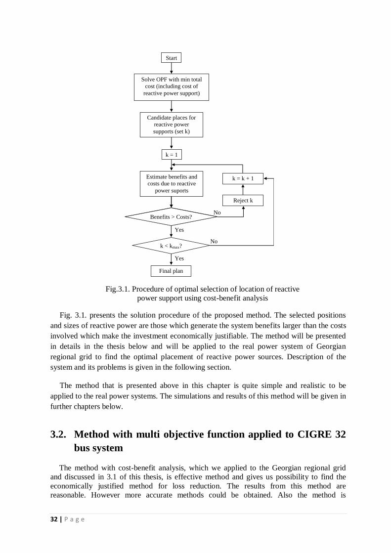
Fig.3.1. Procedure of optimal selection of location of reactive
power support using cost-benefit analysis
Fig. 3.1. presents the solution procedure of the proposed method. The selected positions
and sizes of reactive power are those which generate the system benefits larger than the costs
involved which make the investment economically justifiable. The method will be presented
in details in the thesis below and will be applied to the real power system of Georgian
regional grid to find the optimal placement of reactive power sources. Description of the
system and its problems is given in the following section.
The method that is presented above in this chapter is quite simple and realistic to be
applied to the real power systems. The simulations and results of this method will be given in
further chapters below.
3.2. Method with multi objective function applied to CIGRE 32
bus system
The method with cost-benefit analysis, which we applied to the Georgian regional grid
and discussed in 3.1 of this thesis, is effective method and gives us possibility to find the
economically justified method for loss reduction. The results from this method are
reasonable. However more accurate methods could be obtained. Also the method is
No
Yes
Yes
No
Start
Solve OPF with min total
cost (including cost of
reactive power support)
Candidate places for
reactive power
supports (set k)
k = 1
Estimate benefits and
costs due to reactive
power suports
Benefits > Costs?
Reject k
k = k + 1
Final plan
k < kmax?
Benefits > Costs?

33 | P a g e
optimizing single objective and we are not able to consider two or more objectives, which
represents our interest, while finding optimal solution.
In this thesis another method for optimizing several objective functions will be presented
also. The method includes the multi objective function and it optimizes four objective
functions at the same time.
The objective functions have been chosen considering the most prioritized problems of the
discussed Georgian power system and at the same time the general problems of almost all
power systems. The optimized objective functions, which we are optimizing, are F1, F2, F3
and F4. These objective functions are total investment, average voltage deviation, total active
power losses and total system cost respectively.
The objective functions are defined as follows:
The objective function for total investment, F1, is defined with the same way as in
equation (2.2) in [19]:
Where as in [19] F1 is the total required investment, Bi is the compensation at busbar i in
MVAr, F1m is maximum amount available for investment and Bm is the maximum amount of
compensation allowed at bus i. n represents the number of busses in investigated grid.
The second objective function F2 represents the average voltage deviation. This objective
function is defined as follows:
Where Vi is the actual voltage at bus i in per unit and Vi* is the desired voltage at bus i.
Minimizing this objective function would lead us to improving of voltage levels at each bus.
Third objective function F3, that we will optimize, is minimizing of total losses and it’s
defined with the similar equation as equation (2.1), which is taken from [13]:
Where Gi,j is the conductance of the line i-j, Vi and Vj are line voltages and δi and δj the
line angles at the line i and j ends respectively.
The forth objective function F4 is the total system cost. Equation for the total system cost
is taken from [13] and it’s defined as follows:
34 | P a g e
Here NG is the set of all generating units, Ci is the price of energy at bus i and Pi is the
power, generated at bus i.
For optimizing all these four objective functions at the same time, we use the following
equation:
Here J is the overall objective function that optimizes the above mentioned objective
functions F1, F2, F3 and F4. The multipliers α, δ, and ε are the priority order multipliers by
which we can set the priority orders of the objective functions, that are optimized. The sum
of priority order multipliers is 100%:
α + δ + + ε = 100% (3.6)
F1, F2, F3 and F4 are the objective functions as described in this chapter above. F1*, F2
*, F3
*
and F4* are the optimal values of objective functions F1, F2, F3 and F4 respectively.
Beside the equations for objective functions we are using the general load flow equations
for active and reactive powers, which has been described in chapter two of this thesis:
Where V is bus voltage, δ is the angle associated with V, Yi,j is the element of bus
admittance matrix, θ is the angle associated with Yi,j, P and Q are the active and reactive
power generations respectively, PD and QD are the active and reactive power consumptions
respectively.
Formulation of the multi objective function as it is given in equation (3.5) gives us
opportunity to optimize several objective functions at the same time. During optimization we
have possibility to set the priority order of the objective functions and to put them according
to the importance for us.
The optimal power flow with above defined multi objective function is solved using the
non linear programming solver of [22] below. For the purpose of testing of our developed
method it will be applied to CIGRE 32 bus system [23]. The application procedures and
results are given in further chapters.

35 | P a g e
Chapter 4 Simulations with
Real Networks To be able to test the theory the best way is to apply it to practice. To illustrate our
developed methods, we applied them to the real power systems.
In this chapter modeling, solving strategy and solution results description, review and
result analysis are given for Georgian regional grid and for CIGRE 32 bus system.
4.1. Simulations with Georgian regional grid
The real network of Georgian regional power grid was chosen as a test power network.
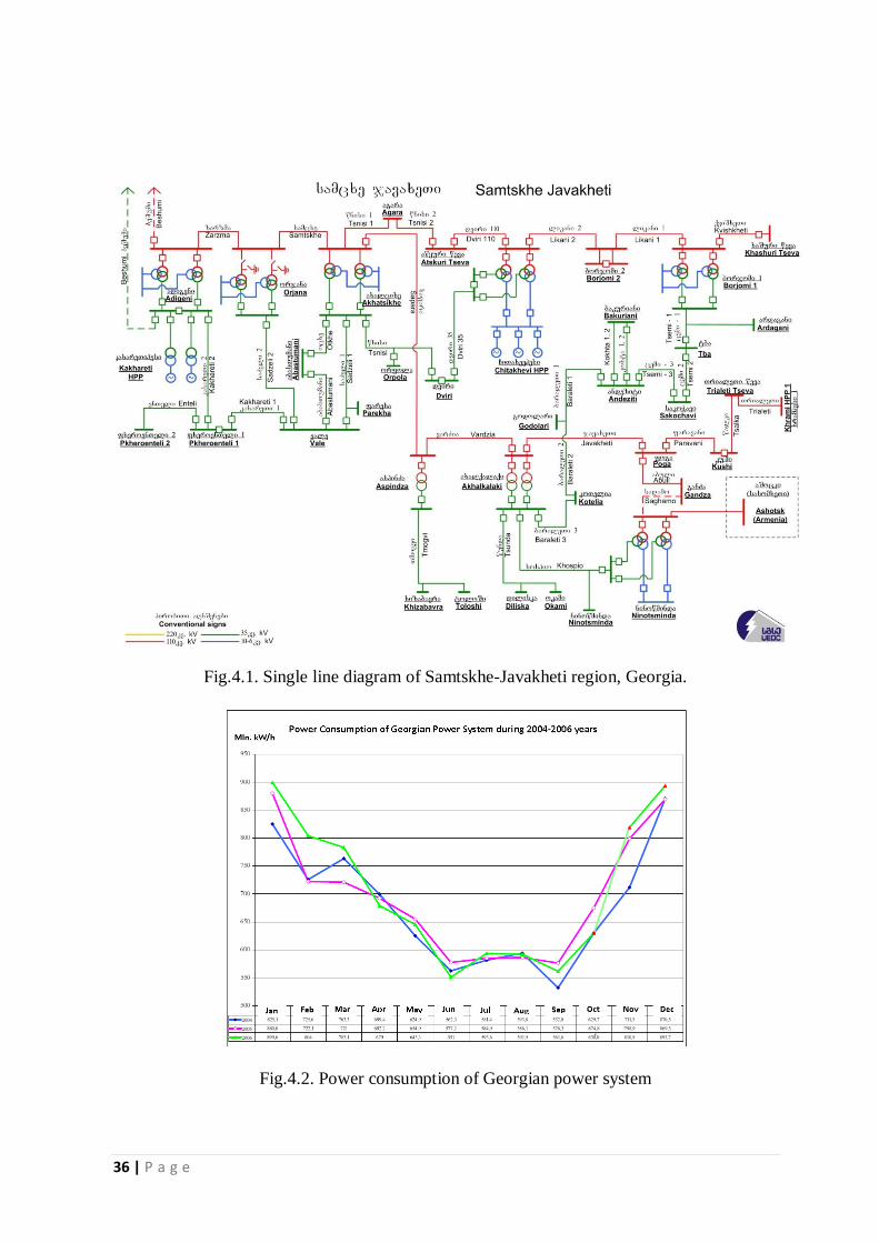
The single line diagram of the network is given at figure 4.1. below. This regional network
can be assumed as the typical for the whole country’s network in terms of its existing
problems and design.
4.1.1. Description of investigated Georgian regional grid
The technical losses are one of the serious problems for the investigated Samtskhe-
Javakheti regional network and for Georgian power system in general. The power system is
old and mostly uncompensated in terms of reactive power. Due to the not adequate planning
most of the equipments like transmission lines and transformers are overloaded during the
peak-hours. Also many transmission lines are not the sizes that they are designed to be. As a
result there are very high losses and serious voltage drops at the ends of the lines in a system
beside of other problems that cause many technical problems in the system in general.
The problem of line overloading, voltage drops and technical losses becomes more
problematic during the heavy load seasons. For Georgian power system such season is
winter. As we can see on fig.4.2, which is taken from [11]
36 | P a g e
Fig.4.1. Single line diagram of Samtskhe-Javakheti region, Georgia.
Fig.4.2. Power consumption of Georgian power system

37 | P a g e
During the power deficit, mainly in winter, in heavy load seasons, sometimes Georgia is
importing the electrical energy from Armenia through the region, which is chosen by us for
investigation. Here the losses are extremely high. The reason is that the imported power is
transmitted through the grid in not optimal way. The imported power is passing from 110 kV
substation ―Ninotsminda‖ to another 110 kV substation ―Akhalkalaki‖ through the 35 kV
line, what makes the 35 kV line overloaded. Normally the grid is fed from 110 kV
―Khashuri-Tseva‖ substation and from hydro power plants (See Fig.4.1.). Owner utility
makes investigations about amount of losses and levels of voltage drops of its system and
about ways of their reduction. According to the utility’s data, losses are 2.9%; 4.2% and
8.2% for 110 kV, 35 kV and 10/6 kV voltage levels, respectively. The highest losses are
observed during the peak hour operations, when the loading of the system is highest. The
typical loading shape for the discussed system is taken from utility’s data [9] and is shown at
fig.4.3 below. The loading shape on fig.4.3 can be approximated as typical shape for whole
Georgian distribution system.
Fig.4.3. Hourly load versus hours of the day
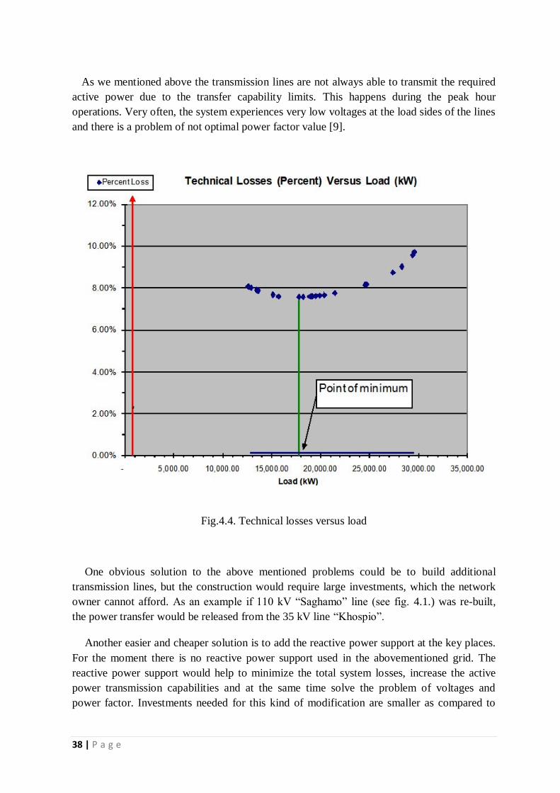
The technical losses versus load are shown in fig. 4.4. The curve on fig.4.4 can also be
assumed as typical for all Georgian power networks. It can be observed from fig. 4.4 that the
losses do not increase linearly with the increase in total system load, but there is certain
minimum of losses, which is occurring somewhere between very light and heavy loads.
38 | P a g e
As we mentioned above the transmission lines are not always able to transmit the required
active power due to the transfer capability limits. This happens during the peak hour
operations. Very often, the system experiences very low voltages at the load sides of the lines
and there is a problem of not optimal power factor value [9].
Fig.4.4. Technical losses versus load
One obvious solution to the above mentioned problems could be to build additional
transmission lines, but the construction would require large investments, which the network
owner cannot afford. As an example if 110 kV ―Saghamo‖ line (see fig. 4.1.) was re-built,
the power transfer would be released from the 35 kV line ―Khospio‖.
Another easier and cheaper solution is to add the reactive power support at the key places.
For the moment there is no reactive power support used in the abovementioned grid. The
reactive power support would help to minimize the total system losses, increase the active
power transmission capabilities and at the same time solve the problem of voltages and
power factor. Investments needed for this kind of modification are smaller as compared to

39 | P a g e
those required for the construction of new lines and the resulting reduced total system losses
can help recover the investments in a shorter time in case of appropriate planning.
4.1.2. Power system modeling and simulation for Georgian regional
grid
In our study, we will model the Georgian regional grid with the three voltage levels of 6-
10 kV, 35kV and 110kV. The data for the system is taken from [9] and the power flow
simulation software CYME [10] will be used for execution of various optimal power flow
solutions required in our proposed method to select the optimal position of reactive power
supports.
As it was mentioned above, the regional grid is fed in two ways. Both ways of feeding are
shown on Fig. 4.5 and Fig. 4.6. According to in which way the grid is fed, two models of our
investigated grid are made.
In Case-1, which will be discussed below, the regional grid is fed through the 110 kV line,
coming from the neighbor country as we can observe from the single line diagram (Fig. 4.5.).
Fig.4.5. Losses and candidate places for reactive power supports for Case-1
Total MW Generation: 27.888MW
Total MW Losses: 2.532MW
Losses in Percentage: 9.08%
Candidate Place N 4
Candidate Place N 5
Candidate Place N 1
Candidate Place N 6 Candidate Place N 2 Candidate Place N 3
Feeding from
Ashotsk 110kV line
40 | P a g e
The imported energy in this case is more expensive than locally produced, but in the case
of power deficit, this way of feeding is the solution for the owner utility. On the single line
diagram we can observe, that the 110 kV line, which is used for import of energy feeds
110/35/10.5 kV substation, which feeds the whole grid through the 35 kV line. This line by
itself is not designed for transmission of such large amount of power. Therefore, it is
becoming overloaded. As a result, we can observe that the total system loss for this case is
9.08%, which is a very high value.
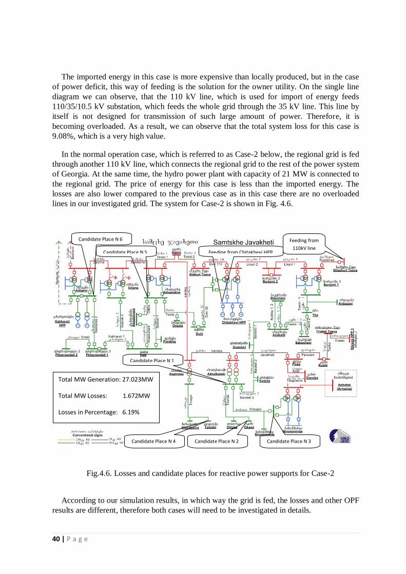
In the normal operation case, which is referred to as Case-2 below, the regional grid is fed
through another 110 kV line, which connects the regional grid to the rest of the power system
of Georgia. At the same time, the hydro power plant with capacity of 21 MW is connected to
the regional grid. The price of energy for this case is less than the imported energy. The
losses are also lower compared to the previous case as in this case there are no overloaded
lines in our investigated grid. The system for Case-2 is shown in Fig. 4.6.
Fig.4.6. Losses and candidate places for reactive power supports for Case-2
According to our simulation results, in which way the grid is fed, the losses and other OPF
results are different, therefore both cases will need to be investigated in details.
Total MW Generation: 27.023MW
Total MW Losses: 1.672MW
Losses in Percentage: 6.19%
Candidate Place N 5
Candidate Place N 6
Feeding from Chitakhevi HPP
Feeding from
110kV line
Candidate Place N 1
Candidate Place N 4 Candidate Place N 2 Candidate Place N 3
41 | P a g e
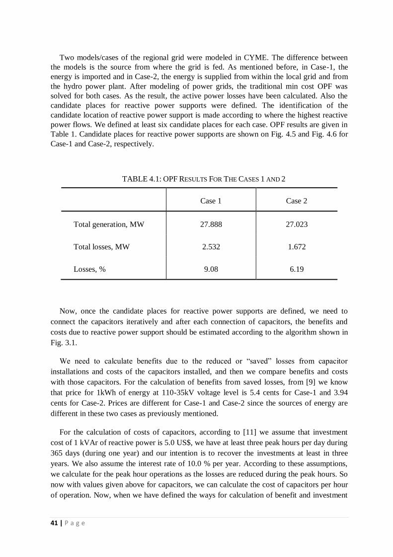
Two models/cases of the regional grid were modeled in CYME. The difference between
the models is the source from where the grid is fed. As mentioned before, in Case-1, the
energy is imported and in Case-2, the energy is supplied from within the local grid and from
the hydro power plant. After modeling of power grids, the traditional min cost OPF was
solved for both cases. As the result, the active power losses have been calculated. Also the
candidate places for reactive power supports were defined. The identification of the
candidate location of reactive power support is made according to where the highest reactive
power flows. We defined at least six candidate places for each case. OPF results are given in
Table 1. Candidate places for reactive power supports are shown on Fig. 4.5 and Fig. 4.6 for
Case-1 and Case-2, respectively.
TABLE 4.1: OPF RESULTS FOR THE CASES 1 AND 2
Case 1 Case 2
Total generation, MW 27.888 27.023
Total losses, MW 2.532 1.672
Losses, % 9.08 6.19
Now, once the candidate places for reactive power supports are defined, we need to
connect the capacitors iteratively and after each connection of capacitors, the benefits and
costs due to reactive power support should be estimated according to the algorithm shown in
Fig. 3.1.
We need to calculate benefits due to the reduced or ―saved‖ losses from capacitor
installations and costs of the capacitors installed, and then we compare benefits and costs
with those capacitors. For the calculation of benefits from saved losses, from [9] we know
that price for 1kWh of energy at 110-35kV voltage level is 5.4 cents for Case-1 and 3.94
cents for Case-2. Prices are different for Case-1 and Case-2 since the sources of energy are
different in these two cases as previously mentioned.
For the calculation of costs of capacitors, according to [11] we assume that investment
cost of 1 kVAr of reactive power is 5.0 US$, we have at least three peak hours per day during
365 days (during one year) and our intention is to recover the investments at least in three
years. We also assume the interest rate of 10.0 % per year. According to these assumptions,
we calculate for the peak hour operations as the losses are reduced during the peak hours. So
now with values given above for capacitors, we can calculate the cost of capacitors per hour
of operation. Now, when we have defined the ways for calculation of benefit and investment

42 | P a g e
cost of the reactive power support, we can start iterations and applying capacitors according
to the flowchart on Fig. 3.1.
In our iterations we will choose the certain sizes of capacitors. These sizes will be
obtained as a result of trial and error which leads us to choosing the final optimal sizes of
capacitors.
4.1.3.Simulation results and their analysis for Georgian regional
grid
Many iterations of OPF have been performed. However, only the significant iterations will
be shown in the following sub-sections.
Iterative simulations for Case-I
Step-1: We install the capacitor of 7.9 MVAr at the candidate place N1 as indicated
on the diagram in Fig. 4.5. Perform an OPF run, and calculate the total system loss.
As a result of capacitor installation, the loss was decreased from 2.532 MW (9.08%)
to 2.194 MW (7.96%). This means that benefit per hour with loss reduction per peak
hour is therefore estimated as 338 kWh x 5.4 cents/kWh = $18.25. The cost of 7.9
MVAr of reactive power support is calculated to be $12.02 per peak-hour. As a result
we have positive net benefit due to reactive power addition since the benefit is greater
that the cost. This means that this case is successful and worthwhile for
implementation.
Step-2: We install a capacitor of 7.4 MVAr at the candidate position N1 and a
capacitor of 1.1 MVAr at the candidate position N2 as indicated in Fig. 4.5. Again we
perform an OPF execution, the losses in this case will be decreased from 2.532 MW
(9.08%) to 2.186 MW (7.92%). Similar to Step-1, in this case the benefit due to loss
reduction per peak hour is calculated to be $18.68. The cost of 7.4 MVAr and 1.1
MVAr of reactive power support is calculated to be $12.94 per peak-hour. This case is
also successful as the benefit is greater than the cost ($18.68 > $12.94).
Step-3: We install a capacitor of 6.8 MVAr at the candidate place N1, and a capacitor
of 2.4 MVAr at the candidate place N2. We will be able to reduce the losses by with
353 kW per hour. The benefit per hour is again calculated to be $19.06. The cost of
reactive power in this case is calculated to be $13.084. This case is successful as the
benefit is greater than the cost ($19.06 > $13.084). This means that this case is also
successful.
Step-4: It is still possible to reduce the loss a bit more than that of the previous step.
We need to add at the candidate place N1 the capacitor of 6.1 MVAr, at the candidate
place N3 5.1 MVAr, and candidate place N4 2.4 MVAr. With this modification, the
loss could be reduced to 2.165MW (7.76%). The benefit per peak hour is $19.82. The
cost is $20.67. However, this case is not successful since the benefit is less than the
cost.

43 | P a g e
Step-5: There is possibility to reduce losses maximally. For this we need to add the
reactive power as follows: at the candidate place N1 – 3.2 MVAr, at the candidate
place N2 – 0.7 MVAr, at the candidate place N3 -7.7 MVAr, at the candidate place
N4 – 4.0 MVAr. With this way, the losses are reduced to 2.163 MW (7.76%). The
benefit per peak hour is $19.93. The cost of reactive power will be $23.74. This case
is again not successful since the benefit is less than the cost ($19.82 < $23.74), even
the losses could be maximally reduced.
As a result of iterations we could observe, that insertion of reactive power at candidate
places N1 and N2 gave us successful results, while addition of capacitors at other candidate
places were not successful even this action reduced losses more. For this case candidate
places N1 and N2 will be chosen for successful addition of reactive power as only in this
case the loss reduction becomes beneficial.
Iterative simulations for Case-II
In this case the grid is fed from the hydro power plant (3X7MW) and from the grid at
the same time. As in previous case the basic optimal power flow was solved for this
case also and active power losses have been calculated. Total generation is 27.027MW
and total active power losses are 1.672MW (6.19%). The candidate places for reactive
power supports were found. All these results are shown on single line diagram on Fig.
4.6.
Step-1: In case if we apply the reactive power of 10MVAr at candidate place N1 as
shown on the diagram in Fig. 4.6, and perform an OPF run, then calculate the total
system loss, the losses will be reduced from 1.672MW (6.19%) to 1.273MW (4.78%).
With this modification we save $15.72 per peak hour. The cost of reactive power
addition per peak hour is $15.22. For this case the benefit is more than the cost ($15.72
> $15.22), that means that this iteration is successful.
Step-2: In this iteration we apply the capacitor of 7.5MVAr at candidate place N1 and
5.4MVAr at candidate place N6 as indicated on the diagram in Fig. 4.6. In such a way
we obtain the loss reduction from 1.672MW (6.19%) to 1.205MW (4.54%). It means
that we save $18.4 per peak hour. Investment due to reactive power addition will be
$19.63 per peak hour. Comparison of benefit with cost shows that cost needed for such
modification is more than benefit. It means that this case is not successful and
worthwhile.
Step-3: Now we install the capacitors of 5.6MVAr at candidate place N1, capacitor of
5.9MVAr at candidate place N5 and capacitor of 3.8MVAr at candidate place N6.
With this modification we gain loss reduction from 1.672MW (6.19%) to 1.180MW
(4.45%) and we save $19.39 per peak hour. The total cost of capacitors addition is
$23.26 per peak hour. Comparison of benefit and cost shows that cost in this case is
more than the benefit that means that this iteration is not successful.
Step-4: We apply the capacitors at the following places: Candidate place N1 –
4.2MVAr; candidate place N3 – 2.4MVAr; candidate place N5 – 5.9MVAr. With this
change we have loss reduction from 1.672MW (6.19%) to 1.198MW (4.5%) and we
44 | P a g e
save $18.68 per peak hour. The total cost of capacitors addition is $19 per peak hour.
This iteration can’t be successful as the cost is more than the benefit.
Step-5: In this case we gain the maximum loss reduction. We apply the capacitors at
the following places: Candidate place N1 – 5.1MVAr; candidate place N2 – 0.3MVAr;
candidate place N3 – 1.7MVAr; candidate place N4 – 1.1MVAr; candidate place N5 –
1.7MVAr; candidate place N6 – 3.7MVAr. With all these capacitors addition we get
loss reduction from 1.672MW (6.19%) to 1.165MW (4.4%) and we save $19.98 per
peak hour. The total cost of capacitors addition is $20.7 per peak hour. For this
iteration the cost is more than the benefit that means that this iteration is not
successful.
Iterative simulations for case-II showed us that insertion of reactive power was successful
only in case if we insert the capacitors at candidate place N1. All the other cases were not
successful and beneficial, even the loss reduction was more. As a result we conclude that for
this case of iterations the successful place for reactive power placement is candidate place
N1.
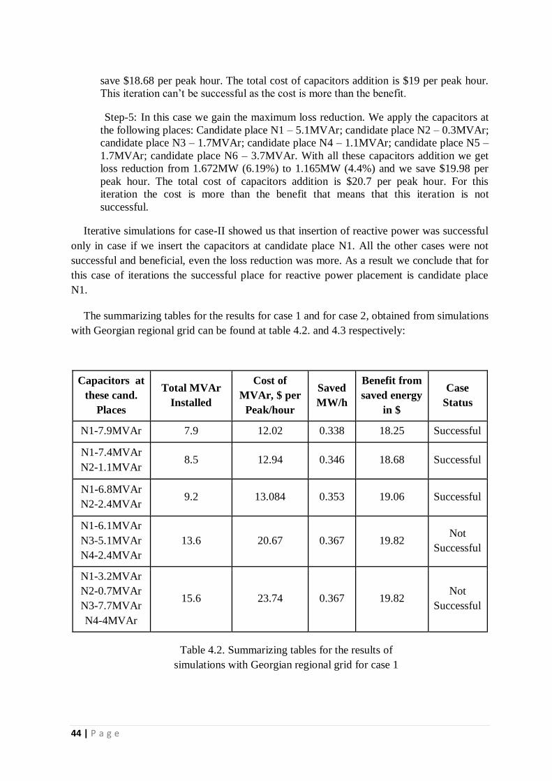
The summarizing tables for the results for case 1 and for case 2, obtained from simulations
with Georgian regional grid can be found at table 4.2. and 4.3 respectively:
Capacitors at
these cand.
Places
Total MVAr
Installed
Cost of
MVAr, $ per
Peak/hour
Saved
MW/h
Benefit from
saved energy
in $
Case
Status
N1-7.9MVAr 7.9 12.02 0.338 18.25 Successful
N1-7.4MVAr
N2-1.1MVAr 8.5 12.94 0.346 18.68 Successful
N1-6.8MVAr
N2-2.4MVAr 9.2 13.084 0.353 19.06 Successful
N1-6.1MVAr
N3-5.1MVAr
N4-2.4MVAr
13.6 20.67 0.367 19.82 Not
Successful
N1-3.2MVAr
N2-0.7MVAr
N3-7.7MVAr
N4-4MVAr
15.6 23.74 0.367 19.82 Not
Successful
Table 4.2. Summarizing tables for the results of
simulations with Georgian regional grid for case 1
45 | P a g e
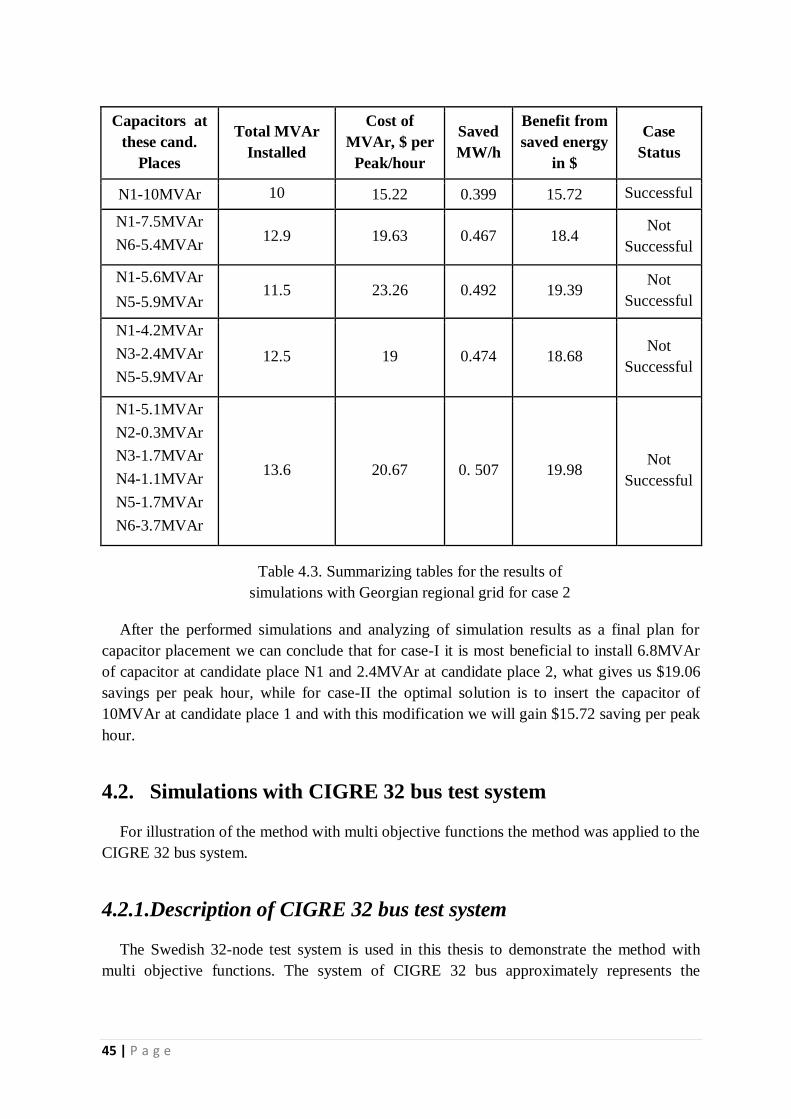
Capacitors at
these cand.
Places
Total MVAr
Installed
Cost of
MVAr, $ per
Peak/hour
Saved
MW/h
Benefit from
saved energy
in $
Case
Status
N1-10MVAr 10 15.22 0.399 15.72 Successful
N1-7.5MVAr
N6-5.4MVAr 12.9 19.63 0.467 18.4 Not
Successful
N1-5.6MVAr
N5-5.9MVAr 11.5 23.26 0.492 19.39
Not
Successful
N1-4.2MVAr
N3-2.4MVAr
N5-5.9MVAr
12.5 19 0.474 18.68 Not
Successful
N1-5.1MVAr
N2-0.3MVAr
N3-1.7MVAr
N4-1.1MVAr
N5-1.7MVAr
N6-3.7MVAr
13.6 20.67 0. 507 19.98 Not
Successful
Table 4.3. Summarizing tables for the results of
simulations with Georgian regional grid for case 2
After the performed simulations and analyzing of simulation results as a final plan for
capacitor placement we can conclude that for case-I it is most beneficial to install 6.8MVAr
of capacitor at candidate place N1 and 2.4MVAr at candidate place 2, what gives us $19.06
savings per peak hour, while for case-II the optimal solution is to insert the capacitor of
10MVAr at candidate place 1 and with this modification we will gain $15.72 saving per peak
hour.
4.2. Simulations with CIGRE 32 bus test system
For illustration of the method with multi objective functions the method was applied to the
CIGRE 32 bus system.
4.2.1.Description of CIGRE 32 bus test system
The Swedish 32-node test system is used in this thesis to demonstrate the method with
multi objective functions. The system of CIGRE 32 bus approximately represents the
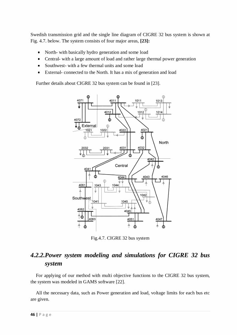
46 | P a g e
Swedish transmission grid and the single line diagram of CIGRE 32 bus system is shown at
Fig. 4.7. below. The system consists of four major areas, [23]:
North- with basically hydro generation and some load
Central- with a large amount of load and rather large thermal power generation
Southwest- with a few thermal units and some load
External- connected to the North. It has a mix of generation and load
Further details about CIGRE 32 bus system can be found in [23].
Fig.4.7. CIGRE 32 bus system
4.2.2.Power system modeling and simulations for CIGRE 32 bus
system
For applying of our method with multi objective functions to the CIGRE 32 bus system,
the system was modeled in GAMS software [22].
All the necessary data, such as Power generation and load, voltage limits for each bus etc
are given.
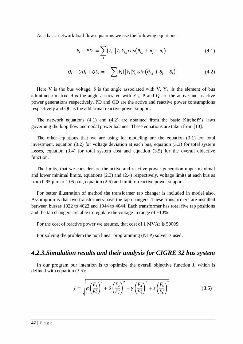
47 | P a g e
As a basic network load flow equations we use the following equations:
Here V is the bus voltage, δ is the angle associated with V, Yi,j is the element of bus
admittance matrix, θ is the angle associated with Yi,j, P and Q are the active and reactive
power generations respectively, PD and QD are the active and reactive power consumptions
respectively and QC is the additional reactive power support.
The network equations (4.1) and (4.2) are obtained from the basic Kirchoff’s laws
governing the loop flow and nodal power balance. These equations are taken from [13].
The other equations that we are using for modeling are the equation (3.1) for total
investment, equation (3.2) for voltage deviation at each bus, equation (3.3) for total system
losses, equation (3.4) for total system cost and equation (3.5) for the overall objective
function.
The limits, that we consider are the active and reactive power generation upper maximal
and lower minimal limits, equations (2.3) and (2.4) respectively, voltage limits at each bus as
from 0.95 p.u. to 1.05 p.u., equation (2.5) and limit of reactive power support.
For better illustration of method the transformer tap changer is included in model also.
Assumption is that two transformers have the tap changers. These transformers are installed
between busses 1022 to 4022 and 1044 to 4044. Each transformer has total five tap positions
and the tap changers are able to regulate the voltage in range of ±10%.
For the cost of reactive power we assume, that cost of 1 MVAr is 5000$.
For solving the problem the non linear programming (NLP) solver is used.
4.2.3.Simulation results and their analysis for CIGRE 32 bus system
In our program our intention is to optimize the overall objective function J, which is
defined with equation (3.5):

48 | P a g e
For solving this equation, as a first step we need to find the optimal values F1*, F2
*, F3
* and
F4* that are the optimal values for total investment in reactive power, total system losses,
voltage deviation at each bus and for total system cost respectively.
First we solve the OPF for the optimal value of total investment in reactive power, F1*.
The obtained results are as follows:
The voltages at each bus after solving for optimal value of total investment in reactive
power are given at figure 4.8.
Fig.4.8. Voltages in p.u. at each bus after solving for optimal
value of total investment in reactive power, F1*
The reactive power support is installed at only one location, at bus 1011 with the amount
of 0.29256580 p.u.
The total system losses for this case are 9.10474333 p.u. and the optimal value of the
investment is F1*=146282.9 $.
As we can observe at figure 4.8., the voltages are just in limits, from 0.95 to 1.05 p.u., but
they have quite big deviation from the ideal voltage value, from 1 p.u. This is what we can
expect from the minimization of investment costs, voltages are just in limits, losses are more
or less acceptable and the minimum required number of reactive power support is allocated at
only one bus, at bus 1011.
The next optimal value that we need to find is the optimal value for losses, F2*. After
solving the OPF for optimal value for losses we obtain the results, which are given and
discussed below:
0.9
0.95
1
1.05
41
42
43
46
47
51
61
62
63
10
11
10
12
10
13
10
14
10
21
10
22
10
41
10
42
10
43
10
44
10
45
20
31
20
32
40
11
40
12
40
21
40
22
40
31
40
32
40
41
40
42
40
43
40
44
40
45
40
46
40
47
40
51
40
61
40
62
40
63
40
71
40
72
Bus Voltages (p.u.)
Bus Voltages (p.u.)

49 | P a g e
The voltages at each bus are as shown at figure 4.9.
Fig.4.9. Voltages in p.u. at each bus after solving for optimal value for losses, F2*
The reactive power support has been applied at total nine different locations in the system,
for gaining the minimal value of losses. The amounts and locations of reactive power
supports are given in figure 4.10.
Fig.4.10. Reactive Power Support allocation and amounts
after solving for optimal value of losses, F2*
0.9
0.95
1
1.05
41
42
43
46
47
51
61
62
63
10
11
10
12
10
13
10
14
10
21
10
22
10
41
10
42
10
43
10
44
10
45
20
31
20
32
40
11
40
12
40
21
40
22
40
31
40
32
40
41
40
42
40
43
40
44
40
45
40
46
40
47
40
51
40
61
40
62
40
63
40
71
40
72
Bus Voltages (p.u.)
Column1
0
0.5
1
1.5
2
2.5
3
3.5
4
41
42
43
46
47
51
61
62
63
10
11
10
12
10
13
10
14
10
21
10
22
10
41
10
42
10
43
10
44
10
45
20
31
20
32
40
11
40
12
40
21
40
22
40
31
40
32
40
41
40
42
40
43
40
44
40
45
40
46
40
47
40
51
40
61
40
62
40
63
40
71
40
72
Reactive Power (p.u.)
Reactive Power p.u.

50 | P a g e
The optimal value of total system losses are: F2*= 4.96669474 p.u.
The optimal value of total system losses are less than half as it was for the case when we
solved OPF for optimal value of total investment in reactive power, F1*. This is obviously
good result, but to reach this optimization, program was obliged to allocate the reactive
power support in nine different locations. Even though the losses are minimized, still the
voltage deviation is quite high from ideal value, 1 p.u. but looks better than it was in previous
case, when we solved OPF for optimal value of total investment in reactive power, F1*.
The next step is to find the optimal value of voltage deviation, F3*. The voltage deviation
is defined with the equation (3.2.). Our objective function is to minimize F3*, that would lead
us to the maximal improvement of voltage levels at each bus.
After solving the OPF for optimal value of voltage deviation, F3*, we obtain the results,
which are shown and analyzed below:
Fig.4.11. Voltages in p.u. at each bus after solving
for optimal value of voltage deviation, F3*
As we can observe, the voltage levels here are very close to desired value, 1 p.u. Only at
several buses it was impossible for the program to optimize the voltage level more.
From figure 4.12. we note, that for reaching the minimal deviation of voltages at each bus,
the program needed to allocate quite high number and value of reactive power.
As a result the losses are 9.50988771 p.u. and the optimal value of voltage deviation,
F3*=0.07906289 p.u. This is quite satisfying value for us.
0.90.920.940.960.98
11.021.04
41
42
43
46
47
51
61
62
63
10
11
10
12
10
13
10
14
10
21
10
22
10
41
10
42
10
43
10
44
10
45
20
31
20
32
40
11
40
12
40
21
40
22
40
31
40
32
40
41
40
42
40
43
40
44
40
45
40
46
40
47
40
51
40
61
40
62
40
63
40
71
40
72
Bus Voltages (p.u.)
Voltages p.u.
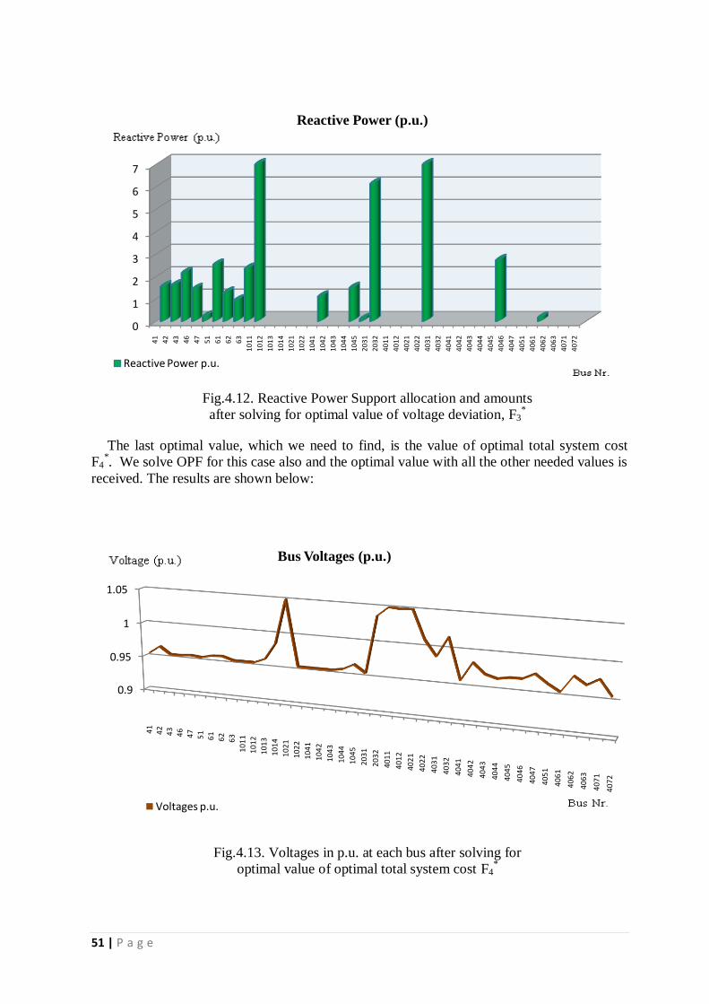
51 | P a g e
Fig.4.12. Reactive Power Support allocation and amounts
after solving for optimal value of voltage deviation, F3*
The last optimal value, which we need to find, is the value of optimal total system cost
F4*. We solve OPF for this case also and the optimal value with all the other needed values is
received. The results are shown below:
Fig.4.13. Voltages in p.u. at each bus after solving for
optimal value of optimal total system cost F4*
0
1
2
3
4
5
6
7
41
42
43
46
47
51
61
62
63
10
11
10
12
10
13
10
14
10
21
10
22
10
41
10
42
10
43
10
44
10
45
20
31
20
32
40
11
40
12
40
21
40
22
40
31
40
32
40
41
40
42
40
43
40
44
40
45
40
46
40
47
40
51
40
61
40
62
40
63
40
71
40
72
Reactive Power (p.u.)
Reactive Power p.u.
0.9
0.95
1
1.05
41
42
43
46
47
51
61
62
63
10
11
10
12
10
13
10
14
10
21
10
22
10
41
10
42
10
43
10
44
10
45
20
31
20
32
40
11
40
12
40
21
40
22
40
31
40
32
40
41
40
42
40
43
40
44
40
45
40
46
40
47
40
51
40
61
40
62
40
63
40
71
40
72
Bus Voltages (p.u.)
Voltages p.u.
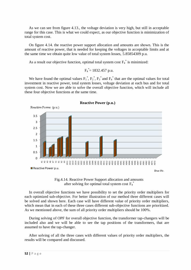
52 | P a g e
As we can see from figure 4.13., the voltage deviation is very high, but still in acceptable
range for this case. This is what we could expect, as our objective function is minimization of
total system cost.
On figure 4.14. the reactive power support allocation and amounts are shown. This is the
amount of reactive power, that is needed for keeping the voltages in acceptable limits and at
the same time we obtain quite low value of total system losses, 5.85854309 p.u.
As a result our objective function, optimal total system cost F4* is minimized:
F4*= 1832.457 p.u.
We have found the optimal values F1*, F2
*, F3
* and F4
* that are the optimal values for total
investment in reactive power, total system losses, voltage deviation at each bus and for total
system cost. Now we are able to solve the overall objective function, which will include all
these four objective functions at the same time.
Fig.4.14. Reactive Power Support allocation and amounts
after solving for optimal total system cost F4*
In overall objective functions we have possibility to set the priority order multipliers for
each optimized sub-objective. For better illustration of our method three different cases will
be solved and shown here. Each case will have different value of priority order multipliers,
which mean that in each of these three cases different sub-objective functions are prioritized.
As we mentioned above, the sum of all priority order multipliers should be 100%.
During solving of OPF for overall objective function, the transformer tap-changers will be
included also and we will be able to see the tap positions of the transformers, that are
assumed to have the tap-changer.
After solving of all the three cases with different values of priority order multipliers, the
results will be compared and discussed.
0
0.5
1
1.5
2
2.5
3
3.5
41
42
43
46
47
51
61
62
63
10
11
10
12
10
13
10
14
10
21
10
22
10
41
10
42
10
43
10
44
10
45
20
31
20
32
40
11
40
12
40
21
40
22
40
31
40
32
40
41
40
42
40
43
40
44
40
45
40
46
40
47
40
51
40
61
40
62
40
63
40
71
40
72
Reactive Power (p.u.)
Reactive Power p.u.

53 | P a g e
Case One
For the first case the priority order multipliers are divided as follows:
Priority order multiplier for investment in reactive power support, α = 10%;
Priority order multiplier for total system losses, δ = 30%;
Priority order multiplier for average voltage deviation at each bus, = 30%;
Priority order multiplier for total system cost, ε = 30%.
For more visibility of division of our interest between priority order multipliers for the
case one the pie chart is given at figure 4.15. below:
Fig.4.15. Division of our interest between
priority order multipliers for the simulation case one
After solving NLP (Non Linear Programming) for minimization of overall objective
function, we obtained the results that are given below:
The voltage levels at each bus are given in figure 4.16.
Fig.4.16. Voltages in p.u. at each bus for case one of optimizing overall objective function
10%
30%
30%
30%
Priority Order Multipliers
Investment α
Losses β
Voltage Deviation γ
Total Cost ε
0.9
0.95
1
1.05
41
42
43
46
47
51
61
62
63
10
11
10
12
10
13
10
14
10
21
10
22
10
41
10
42
10
43
10
44
10
45
20
31
20
32
40
11
40
12
40
21
40
22
40
31
40
32
40
41
40
42
40
43
40
44
40
45
40
46
40
47
40
51
40
61
40
62
40
63
40
71
40
72
Bus Voltages (p.u.)
Voltages p.u.

54 | P a g e
The reactive power allocation and quantities are given in figure 4.17.:
Fig.4.17. Reactive Power Support allocation and amounts after
solving for case one of optimizing overall objective function
Tap Changer positions for the transformers:
Transformer From bus 1022 To bus 4022: Tap Position IV. (105% of nominal
voltage level)
Transformer From bus 1044 To bus 4044: Tap Position II. (95% of nominal
voltage level)
The total system loss for this case is 9.08059016 p.u., the total system cost is 742.5 $ and
the overall objective function, J = 0.00013053 p.u.
As we can observe from the simulation results of case one, the voltage levels are
improved. Only at some busses there are quite high deviations from the desired voltage level,
but in general the voltage levels are in acceptable range. The total system losses are also in
satisfactory level. While improving the voltage levels and reducing the losses, for keeping
the total system cost and investments in reactive power supports on minimal values, the
program allocated minimal reactive power supports in total three different busses.
These results are exactly what we could expect when we divided our interests by priority
order multipliers for the case one.
0
0.5
1
1.5
2
2.5
3
41
42
43
46
47
51
61
62
63
10
11
10
12
10
13
10
14
10
21
10
22
10
41
10
42
10
43
10
44
10
45
20
31
20
32
40
11
40
12
40
21
40
22
40
31
40
32
40
41
40
42
40
43
40
44
40
45
40
46
40
47
40
51
40
61
40
62
40
63
40
71
40
72
Reactive Power (p.u.)
Reactive Power p.u.

55 | P a g e
Case Two
For case two the priority order for total system losses is more prioritized, then the other
multipliers and the other three multipliers are equally divided:
Priority order multiplier for investment in reactive power support, α = 20%;
Priority order multiplier for total system losses, δ = 40%;
Priority order multiplier for average voltage deviation at each bus, = 20%;
Priority order multiplier for total system cost, ε = 20%.
The interest division between priority order multipliers for the case two can be seen better
on the pie chart at figure 4.18. below:
Fig.4.18. Division of our interest between
priority order multipliers for the simulation case two
As in previous case, here we solved the NLP for the overall objective function. The results
of the solution can be found below:
Below the voltage levels at each bus are given:
Fig.4.19. Voltages in p.u. at each bus for case two of optimizing overall objective function
20%
40%20%
20%
Priority Order Multipliers
Investment α
Losses β
Voltage Deviation γ
0.9
0.95
1
1.05
41
42
43
46
47
51
61
62
63
10
11
10
12
10
13
10
14
10
21
10
22
10
41
10
42
10
43
10
44
10
45
20
31
20
32
40
11
40
12
40
21
40
22
40
31
40
32
40
41
40
42
40
43
40
44
40
45
40
46
40
47
40
51
40
61
40
62
40
63
40
71
40
72
Bus Voltages (p.u.)
Voltages p.u.

56 | P a g e
For this case the voltage deviation wasn’t as prioritized as total system losses. As a result
the voltage levels are improved, but at some buses the voltage deviation still remains high. In
general the voltage levels are in acceptable range.
The reactive power allocation and quantities of reactive power for case two can be found
at figure 4.20. below:
Fig.4.20. Reactive Power Support allocation and amounts after
solving for case two of optimizing overall objective function
Tap Changer positions for the transformers are the same as fo the case one and they are as
follows:
Transformer From bus 1022 To bus 4022: Tap Position IV. (105% of nominal
voltage level)
Transformer From bus 1044 To bus 4044: Tap Position II. (95% of nominal
voltage level)
The total system loss for this case is 9.07253424 p.u., the total system cost is 742.5 $ and
the overall objective function, J = 0.00020602 p.u.
The reactive power support has been allocated at the same busses as in previous case, in
case one, but for this case the amount of reactive power is slightly higher. The reason is, that
program tries to minimize the total system losses with this action, and at the same time it’s
not affordable to increase the reactive power more, as in such case the investments will be
higher. As a result the total system losses are decreased compared to case one, while all the
other objective functions are optimized.
All the output results correspond to the division of interest between priority order
multipliers that we gave to the program.
0
0.5
1
1.5
2
2.5
3
41
42
43
46
47
51
61
62
63
10
11
10
12
10
13
10
14
10
21
10
22
10
41
10
42
10
43
10
44
10
45
20
31
20
32
40
11
40
12
40
21
40
22
40
31
40
32
40
41
40
42
40
43
40
44
40
45
40
46
40
47
40
51
40
61
40
62
40
63
40
71
40
72
Reactive Power (p.u.)
Reactive Power p.u.

57 | P a g e
Case Three
One more case with different values of priority order multipliers will be shown below. For
this case our priority is to minimize the losses and not to spend too much investment for
reactive power support. Voltage levels are also important for us, but it will be enough if the
voltages will remain just in their acceptable range. Some attention is paid to the total system
cost also.
The priority order multipliers are divided as follows:
Priority order multiplier for investment in reactive power support, α = 30%;
Priority order multiplier for total system losses, δ = 40%;
Priority order multiplier for average voltage deviation at each bus, = 10%;
Priority order multiplier for total system cost, ε = 20%.
Priority order multipliers for the case three are shown on pie chart at figure 4.21. below:
Fig.4.21. Division of our interest between
priority order multipliers for the simulation case three
We solve NLP and the obtained results are given and discussed below:
Tap Changer positions for the transformers:
Transformer From bus 1022 To bus 4022: Tap Position III. (100% of nominal
voltage level)
Transformer From bus 1044 To bus 4044: Tap Position II. (95% of nominal
voltage level)
The voltages at each bus are given in figure 4.22.
The total system loss here is 8.45444222 p.u., the total system cost is 743.4 $ and the
overall objective function is minimized to: J = 0.00071248 p.u.
Our highest priority for this case was to minimize the total system losses and as we can
see the losses are minimized compared to other three cases. Second priority was to make
30%
40%
10%
20%
Priority Order Multipliers
Investment α
Losses β
Voltage Deviation γ
Total Cost ε

58 | P a g e
minimum investments in reactive power support and as we can observe at figure 4.23. the
minimal amount of reactive support is added to only two locations. The total system cost is
minimized, while the voltage levels are in acceptable ranges.
Fig.4.22. Voltages in p.u. at each bus for case three of
optimizing overall objective function
The reactive power allocation and quantities are given in figure 4.23. below:
Fig.4.23. Reactive Power Support allocation and amounts after
solving for case three of optimizing overall objective function
0.9
0.95
1
1.05
41
42
43
46
47
51
61
62
63
10
11
10
12
10
13
10
14
10
21
10
22
10
41
10
42
10
43
10
44
10
45
20
31
20
32
40
11
40
12
40
21
40
22
40
31
40
32
40
41
40
42
40
43
40
44
40
45
40
46
40
47
40
51
40
61
40
62
40
63
40
71
40
72
Bus Voltages (p.u.)
Voltages p.u.
0
0.05
0.1
0.15
0.2
0.25
0.3
41
42
43
46
47
51
61
62
63
10
11
10
12
10
13
10
14
10
21
10
22
10
41
10
42
10
43
10
44
10
45
20
31
20
32
40
11
40
12
40
21
40
22
40
31
40
32
40
41
40
42
40
43
40
44
40
45
40
46
40
47
40
51
40
61
40
62
40
63
40
71
40
72
Reactive Power (p.u.)
Reactive Power p.u.

59 | P a g e
As we can see, these results are the outputs that correspond to the interests, that we added
to the program, while simulating the case three.
Comparison between the results of simulation cases one, two and three
As we can see, all three simulation cases, where we gave different priorities to different
objective functions, all cases were successful. We were able to see, that the objective
functions, like investment in reactive power support, total system losses, voltage deviation
and total system cost were optimized according to what was our interest in them. The
simulation results are summarized in table 4.4. below:
CASE 1 CASE 2 CASE 3
Total investment (p.u.) 1539718 1540275 151623.6
Average voltage deviation (p.u.) 0.23257235 0.23249908 0.21482606
Total active power losses (p.u.) 9.08059016 9.07253424 8.45444222
Total system cost ($) 742.5 742.5 743.4
Overall Objective function (p.u.) 0.00013053 0.00020602 0.00071248
Table 4.4. Summary for simulation results for method with multi objective functions
In case three the total system losses are lowest compared to other cases, because losses are
prioritized more in case three. The reactive power support is also low for case three and it’s
allocated only at two buses. This is the result of importance of priority order in case three.
In case one and two program tried to minimize the voltage deviation and we can see the
results at figures 4.16. and 4.19. To reach this voltage optimization value and minimization
of total system losses, the reactive power support was allocated at three busses as we can see
at figures 4.17. and 4.20. The reactive power support amount is more, than for case three,
because here, in case one and two the minimization of investments in reactive power were
not as prioritized as in case three.

60 | P a g e

61 | P a g e
Chapter 5 Conclusions
In this thesis, the method for successful capacitor placement with the objective function of
active power losses reduction together with cost-benefit analysis was proposed. The method
was implemented on the example of real power grid of one of the Georgian regions.
As we could observe from our iterations, in case if we make investments for addition of
reactive power in power system for loss reduction objective, reduced losses will easily
recover investment costs caused due to the capacitors addition. However this was not true for
all the cases in our iterations and some cases were not successful and effective. Our
iterations, made on real power grid shows, that in some cases even though the losses are
reduced, the investment cost could be so high, that economically it becomes not effective to
implement such changes. Especially it is true when we maximally reduce losses and for this
we need to apply many sources of reactive power in different locations of the grid. In such
case it becomes even more difficult to operate the number of capacitors as with connection
and disconnections of reactive power sources many factors of power system should be
considered.
However in our iterations we made assumptions regarding the time for the investment
recovery, average peak-hours per day and number of peak-hour days per year as well as the
investment cost for reactive power support addition. If we change these assumptions, then the
results of cost-benefit comparisons will change and unsuccessful iterations could become
successful or vice versa.
Also our suggested method of reactive power addition for the loss reduction purpose
becomes even more effective and economically worthwhile in power systems with higher
loads and where peak-hour operations are longer.
For being able to significantly improve the performance of power systems and to reduce
losses, reactive power should be applied properly and controlled. But if not properly applied
or controlled, the reactive power from capacitor banks can create even more losses and high

62 | P a g e
voltages. The greatest danger of overvoltage occurs under light load. Good planning helps to
ensure that capacitors are placed and operated properly.
In this thesis another method with multi objective functions was introduced and applied to
the CIGRE 32 bus test system. With this method we were able to optimize four objective
functions at the same time. While solving for multi objective function, we were able to set
the priority order of the objective functions that should be optimized. Beside of these
advantages, the method has other advantages also, compared to the method, applied to the
Georgian power grid. Advantages are more accurate results of iterations, as in the method
with multi objective functions the full process of iteration is done by the program and
program can give us the exact locations and sizing of reactive power support, which should
be applied to the system for optimization of initially set multi objective functions.
In our case in method with multi objective functions we optimized only four objective
functions, but optimization of more functions is also possible within the same method.
As a result the methods for proper allocation of reactive power support were developed in
this thesis. Methods include different objectives and consider the financial factors. The
methods, discussed here could be useful for power utilities like Georgian power system,
where the technical losses and voltage drops are causing the problems.

63 | P a g e
Chapter 6 Future work
In this thesis the way of active power loss reduction method with proper application of
reactive power sources to the system is discussed and analyzed. However the method
considers and the simulation has been done only for the peak hour operations, when the
system is heavy loaded. The heavy load can normally last 3-4 hours each day, while during
the rest of the time load is decreased and therefore the system is becoming able to transfer the
needed power without overloading the system components. Accordingly the losses are
becoming lower. In such a case, when the loads are lowered, the reactive power sources,
which we applied to the system during the peak hour operations, become excessive and their
injected reactive power can cause even more losses and destructive overvoltages. Therefore
it’s very important the reactive power sources to be properly operated and switched to the
system only in case when they will be needed, i.e. during the heavy loads of the system.
Another phenomenon to be considered due to the reactive power compensation of the
system is the transients, caused at the moment of connection and reactive power sources. As
it is essential to apply the reactive power sources to the system only during peak-hours, the
problem of transients becomes urgent for consideration while planning the locations and
sizing of reactive power sources.
As a future work the ways to control the reactive power sources should be investigated.
What could be the best way for the control system to sense which reactive power source is
better to connect and when and when it’s best moment to disconnect from the system.
The transients due to the reactive power compensation should be studied also. It should be
investigated what is the maximum number and size of capacitors that could be added to the
certain system without producing the transient problems. Also how serious consequence
can have the case when two or more capacitors are switched on or off at the same time.

64 | P a g e

65 | P a g e
References
[1] Conejo, A.J., Galiana, F.D., and Kockar, I.: ―Z-bus loss allocation‖, IEEE
Transactions on Power Systems, 2001, Vol. 16 No. 1, pp. 105-106.
[2] M. A. Abdel-Moamen, M.A.; N. P. Padhy, Power Flow Control and Transmission
Loss Minimization Model with TCSC for Practical Power Networks‖, IEEE Power
Engineering Society General Meeting, 13-17 July 2003, Vol. 2, pp. 880-884.
[3] K. R. C. Mamandur, and R. D. Chenoweth, ―Optimal Control of Reactive Power
Flow for Improvement in Voltage Profiles and for Real Power Loss Minimization,‖
IEEE Transactions on Power Apparatus and Systems, Vol. PAS-100, No. 7,
pp1509-1515, July 1981.
[4] S. R. Iyer, K. Ramachandran, and S. Hariharan, ―Optimal Reactive Power
Allocation for Improved System Performance,‖ IEEE Transactions on Power
Apparatus and Systems, Vol. PAS-103, No. 6, June 1984
[5] B.F. Wollenberg, ―Transmission system reactive power compensation‖, IEEE
Power Engineering Society Winter Meeting, 27-31 Jan. 2002, vol.1, pp. 507 – 508.
[6] ―Reactive Power Control in Electric Systems‖, Edited by Timothy J. E. Miller, John
Wiley & Sons, New York, 1982.
[7] J.W. Lamont, J. Fu, ―Cost Analysis of Reactive Power Support‖, IEEE
Transactions on Power Systems, Vol. 14, No. 3, pp. 890-895, August 1999.
[8] B. Venkatesh, G. Sadasivam, M.A. Khan, ―A new optimal reactive power
scheduling method for loss minimization and voltage stability margin maximization
using successive multi-objective fuzzy LP technique‖, IEEE Transactions on Power
Systems, Vol. 15, No. 2, May 2000, pp. 844 – 851.
[9] Energo-Pro Georgia’s (UEDC) Technical Department, June 2006.
[10] CYME Power Engineering Solutions. www.cyme.com
[11] Eromon, David I., John Kueck, Oak Ridge, Tom Rizy, Oak Ridge, ―Distributed
Energy Resource (DER) Using FACTS, STATCOM, SVC and Synchronous
condensers for Dynamic Systems Control of VAR‖, National Association of
Industrial Technology (NAIT) Convention, St. Louis, November 16-19, 2005.
[12] Ministry of Energy of Georgia. www.minenergy.gov.ge.
[13] Kankar Bhattacharya, Math H.J. Bollen, Jaap E. Daadler, ―Operation of restructured
power systems‖ by Chalmers University of Technology, Kluver Academic
Publishers, 2001.
[14] Bruce F. Wollenberg, ―Transmission System Reactive Power Compensation‖,
Volume 1, 27-31 Jan. 2002 Page(s):507 - 508 vol.1, Power Engineering Society
Winter Meeting, IEEE, 2002.
[15] ABB brochure, ―Reactive Power-Less is More‖, SECAP A01.en, Edition 2, 2000-
05, pp. 3.
[16] Leonard L Grigsby, Rao S. Thallam, Reactive Power Compensation, ―Electric
Power Generation, Transmission, and Distribution‖ pp. 2, Taylor&Francias Group,
2007.
[17] Short, T. A, ―Electric Power Distribution Equipment and Systems‖ Capacitor
Application, pp. 280-281, Taylor&Francias Group, 2005.
[18] ABB brochure, ―Power capacitors for high and medium voltage application‖. 2006.
Available online: www.abb.com/powercapacitors

66 | P a g e
[19] P. Gardel, B. Baran, H. Estigarribia, U. Fernandez, S. Duarte, ―Multiobjective
Reactive Power Compensation with an Ant Colony Optimization Algorithm‖ IEEE
Transactions on Power Systems, March 2006 Page(s): 276 - 280
[20] Jose Vallejos, Ubaldo Fernandez and Rodrigo Ramos, ―Multiobjective Reactive
Power Compensation Applied to the Paraguayan Power System‖, Transmission &
Distribution Conference and Exposition: Latin America, 2006. TDC '06. IEEE/PES
[21] S. Salamat Sharif, James H. Taylor, Eugene F. Hill, ―On-line Optimal Reactive
Power Flow by Energy Loss Minimization‖, Proceedings of the 35th conference on
decision and control. Kobe, Japan. IEEE, 1996. pp 3851-3856.
[22] General Algebraic Modeling System (GAMS). www.gams.com
[23] K. Walve, "Nordic 32-A CIGRE Test System for Simulation of Transient Stability
and Long Term Dynamics", Svenska Kraftnat, Sweden 1993.
[24] S. Ishak, A. F. Abidin and T. K. A. Rahman, ―Static Var Compensator Planning
Using Artificial Immune System For Loss Minimisation And Voltage
Improvement‖ ‖ IEEE Transactions on Power Systems, 2004, Page(s): 41 – 45.
[25] Dedek Lukman, Trevor R. Blackburn, ―Loss Minimization in Load Flow
Simulation in Power System‖ 4th IEEE International Conference on Power
Electronics and Drive Systems, 2001. Proceedings 2001, Vol.1, pp. 84-88
[26] Stevenson W. D. ―Elements of Power System Analysis‖, 3rd
edition, McGraw-Hill
Kogakusha Ltd, Tokyo, 1975.
[27] Brian Chui G. Shin, ―Development of the Loss Minimization Function for Real
Time Power System Operations: A New Tool‖, IEEE Transactions on Power
Systems, Vol. 9, No. 4. November 1994, pp. 2028-2034.
[28] B. Venkatesh, G. Sadasivam, M. Abdullah Khan, ―A New Optimal Reactive Power
Scheduling Method for Loss Minimization and Voltage Stability Margin
Maximization Using Successive Multi-Objective Fuzzy LP Technique‖, IEEE
Transactions on Power Systems, Vol. 15, No. 2, May 2000, pp.844-851.
67 | P a g e
Appendix A
2007 Large Engineering Systems Conference on Power Engineering
ENERGY FOR THE FUTURE
The Delta Centre-Ville Hotel
October 10 to 12, 2007, Montreal, Quebec, Canada
Optimal Placement of Reactive Power Supports for Transmission
Loss Minimization: The Case of Georgian Regional Power Grid,
Otar Gavasheli and Le Anh Tuan

68 | P a g e
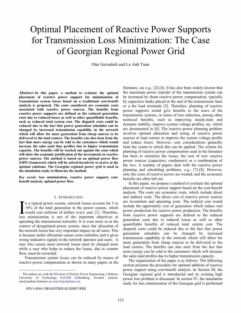
125
Abstract--In this paper, a method to evaluate the optimal placement of reactive power support for minimization of transmission system losses based on a traditional cost-benefit analysis is proposed. The costs considered are economic costs associated with reactive power sources. The benefits from reactive power supports are defined as the reduced generation costs due to reduced losses as well as other quantifiable benefits, such as reduced total system cost. The dispatch costs could be reduced due to the fact that power generation schedules can be changed by increased transmission capability in the network which will allow for more generation from cheap sources to be delivered to the load centers. The benefits can also stem from the fact that more energy can be sold to the customers which would increase the sales (and thus profits) due to higher transmission capacity. The benefits will be worked out against the costs which will show the economic justification of the investments in reactive power sources. The method is based on an optimal power flow (OPF) framework which will be solved iteratively to arrive at the optimal solutions. The Georgian regional power grid is used in the simulation study to illustrate the method.
Key words: loss minimization, reactive power support, cost-benefit analysis, optimal power flow.
I. INTRODUCTION n a typical power system, network losses account for 5 to 10% of the total generation in the power system, which would cost millions of dollars every year [1]. Therefore,
loss minimization is one of the important objectives in operating the transmission networks. It is even more so in the context of deregulated power system, since fair allocation of the network losses has very important impact on all users. This is because unfair allocation causes cross subsidies and it gives wrong indicative signals to the network operator and users. A user who causes more network losses must be charged more while a user who helps to reduce the losses, due to counter flow, must be rewarded.
Transmission system losses can be reduced by means of reactive power compensation as shown in many papers in the
The authors are with the Division of Electric Power Engineering, Chalmers
University of Technology S-41296 Gothenburg, Sweden. (emails: [email protected]; [email protected])
978-1-4244-1583-0/07/$25.00 ©2007 IEEE
literature, see e.g., [2]-[4]. It has also been widely known that the maximum power transfer of the transmission system can be increased by shunt reactive power compensation, typically by capacitors banks placed at the end of the transmission lines or a the load terminals [5]. Therefore, planning of reactive power supports would give benefits to the users of the transmission systems, in terms of loss reduction, among other technical benefits, such as improving steady-state and dynamic stability, improve system voltage profiles, etc. which are documented in [6]. The reactive power planning problem involves optimal allocation and sizing of reactive power sources at load centers to improve the system voltage profile and reduce losses. However, cost considerations generally limit the extent to which this can be applied. The criteria for planning of reactive power compensation used in the literature has been to minimize the losses, the cost of new reactive power sources (capacitors, condensers) or a combination of the two. A number of papers deal with the reactive power planning and scheduling problems, e.g., [7]-[8]. However, only the costs of reactive power are treated, and the economic benefits are often left out.
In this paper, we propose a method to evaluate the optimal placement of reactive power support based on the cost-benefit analysis. The costs are economic costs, which include direct and indirect costs. The direct cost of reactive power sources are investment and operating costs. The indirect cost would include the opportunity cost of generators which reduce real power production for reactive power production. The benefits from reactive power supports are defined as the reduced generation costs due to reduced losses as well as other quantifiable benefits of reduced total system cost. The dispatch costs could be reduced due to the fact that power generation schedules can be changed by increased transmission capability in the network which will allow for more generation from cheap sources to be delivered to the load centers. The benefits can also stem from the fact that more energy can be sold to the customers which will increase the sales (and profits) due to higher transmission capacity.
The organization of the paper is as follows: The following section presents the procedure for optimal addition of reactive power support using cost-benefit analysis. In Section III, the Georgian regional grid is introducted and its existing high power loss problem is discussed. In section IV, the simulation study for loss minimization of the Georgian grid is performed
Optimal Placement of Reactive Power Supports for Transmission Loss Minimization: The Case
of Georgian Regional Power Grid Otar Gavasheli and Le Anh Tuan
I

126
for two possible feeding cases using our propsed methodology. Finally, conclusions are made in Section V.
II. THE PROPOSED SELECTION METHODOLOGY In this method, the candidate positions of reactive power sources will be first identified using an optimal power flow (OPF) framework with the minimum total cost objective including costs of new reactive power sources. The cost-benefit analysis will then be worked out against the candidate locations, with different standard sizes of reactive power sources, so as to arrive at the optimal plan for reactive power support in an iterative manner. Fig. 1 presents the solution procedure of the proposed method. The selected positions and sizes of reactive power are those which generate the system benefits larger than the costs involved which make the investment economically justifiable. The method will be presented in details in the paper and will be applied to the real power system of Georgian regional grid to find the optimal placement of reactive power sources. A brief description of the system and its problems is given in the following section.
No
Yes
Yes
No
Start
Solve OPF with min total cost (including cost of
reactive power support)
Candidate places for reactive power supports (set k)
k = 1
Estimate benefits and costs due to reactive
power suports
Benefits > Costs?
Reject k
k = k + 1
Final plan
k < kmax?
Benefits > Costs?
Fig. 1: Procedure of optimal selection of location of reactive power support using cost-benefit analysis
III. GEORGIAN REGIONAL GRID AND ITS EXISTING PROBLEMS
High power losses is one of the serious problems in the transmission and distribution systems in Georgia, where the power systems are aging and have not been optimized and often uncompensated in terms of reactive power. One typical example is the case of Samtskhe-Javakheti, a regional grid of Georgia. The single-line diagram of this regional grid is given in Fig. 2.
Fig. 2: Single-line diagram of Samtskhe-Javakheti regional grid
Through this region, Georgia is importing the electrical energy from Armenia during the time of power deficit. Here the losses are extremely high. The reason is that the imported power is transited through the grid in not optimal way. Owner utility makes investigations about amount of losses of its system and about ways of their reduction. According to the utility’s data, losses are 2.9%; 4.2% and 8.2% for 110 kV, 35 kV and 10/6 kV voltage levels, respectively. The highest losses are observed during the peak hours, when the loading of the system is high. The typical loading shape for this discussed system is taken from utility’s data [9] and is shown at Fig.3. The technical losses versus load are shown in Fig. 4. It can be observed from Fig. 4 that the loss does not increase linearly with the increase in total system load.

127
Fig.3: Hourly load versus hours of the day
Fig.4: Technical losses versus total system load
Another problem of the system is that the transmission lines are not able to transmit the required active power due to the transfer capability limits. Very often, the system experiences very low voltages at the load sides of the lines and there is a problem of not optimal power factor value [9].
One obvious solution to the above mentioned problems could be to build additional transmission lines, but the construction would require large investments, which the network owner cannot afford. Another easier and cheaper solution is to add the reactive support at the key places. For the moment there is no reactive power support used in the above mention grid. The reactive power support would help to minimize the total system losses, increase the active power transmission capabilities and at the same time solve the problem of voltages and power factor. Investments needed for this kind of modification are smaller as compared to those required for the construction of new lines and the resulting reduced total system losses can help recover the investments in a shorter time in case of appropriate planning as will be shown in the following section.
IV. THE SIMULATION STUDY: GEORGIAN REGIONAL GRID In our study, we will model the Georgian regional grid with the three voltage levels of 6-10 kV, 35kV and 110kV. The data for the system is taken from [9] and the power flow simulation software CYME [10] will be used for execution of various optimal power flow solutions required in our proposed method to select the optimal position of reactive power supports.
The regional grid is fed in two ways. Both ways of feeding are shown on Fig. 5 and Fig. 6. In Case-1, which will be discussed below (Fig. 5), the regional grid is fed through the 110 kV line, coming from the neighbor country.
Fig. 5: Losses and candidate places for reactive power supports for Case-1 The imported energy in this case is more expensive than
locally produced, but in the case of power deficit, this way of feeding is the solution for the owner utility. On the single line diagram we can observe, that the 110 kV line, which is used for import of energy feeds 110/35/10.5 kV substation, which feeds the whole grid through the 35 kV line. This line by itself is not designed for transmission of such large amount of power. Therefore, it is becoming overloaded. As a result, we can observe that the total system loss for this case is 9.08%, which is a very high value.
In the normal operation case, which is referred to as Case-2 below, the regional grid is fed through another 110 kV line, which connects the regional grid to the rest of the power system of Georgia. At the same time, the hydro power plant with capacity of 21 MW is connected to the regional grid. The price of energy for this case is less than the imported energy. The losses are also lower compared to the previous case as in this case there are no overloaded lines in our investigated grid. The system for Case-2 is shown in Fig. 6.

128
Fig. 6: Losses and candidate places for reactive power supports for Case-2 According to our simulation results, in which way the grid
is fed, the losses and other OPF results are different, therefore both cases will need to be investigated in details.
Two models/cases of the regional grid were modeled in CYME. The difference between the models is the source from where the grid is fed. As mentioned before, in Case-1, the energy is imported and in Case-2, the energy is supplied from within the local grid and from the hydro power plant. After modeling of power grids, the traditional min cost OPF was solved for both cases. As the result, the active power losses have been calculated. Also the candidate places for reactive power supports were defined. The identification of the candidate location of reactive power support is made according to where the highest reactive power flows. We defined at least six candidate places for each case. OPF results are given in Table I. Candidate places for reactive power supports are shown on Fig. 5 and Fig. 6 for Case-1 and Case-2, respectively.
TABLE I: OPF RESULTS FOR THE CASES 1 AND 2
Case-1 Case-2
Total generation, MW 27.888 27.023 Total losses, MW 2.532 1.672
Losses, % 9.08 6.19
Once the candidate places for reactive power supports are identified, we need to connect the capacitors iteratively and after each connection of capacitors, the benefits and costs due to reactive power support should be estimated according to the algorithm shown in Fig. 1.
We need to calculate benefits due to the reduced or “saved” losses from capacitor installations and costs of the capacitors installed, and then we compare benefits and costs with those capacitors. For the calculation of benefits from saved losses, from [9] we know that price for 1kWh of energy at 110-35kV voltage level is 5.4 cents for Case-1 and 3.94 cents for Case-2. Prices are different for Case-1 and Case-2 since the sources of energy are different in these two cases as previously mentioned.
For the calculation of costs of capacitors, according to [11] we assume that investment cost of 1 kVAr of reactive power is $5.0, we have at least three peak hours per day during during a year. We assume the economic life of the capacitors is three years. We also assume the interest rate of 10.0 % per year. According to these assumptions, we calculate for the peak hour operations as the losses are reduced during the peak hours. So now with values given above for capacitors, we can calculate the cost of capacitors per hour of operation. Now, when we have defined the ways for calculation of benefit and investment cost of the reactive power support, we can start iterations and applying capacitors according to the flowchart on Fig. 1.
Many iterations of OPF have been performed. However, only the significant iterations will be shown in the following sub-sections. In the iterative calculation, we will choose the certain sizes of capacitors. These sizes of the capacitors were obtained using “trials and errors”, which leads us to choosing the final optimal sizes of capacitors.
A. Iterative simulations for Case-I Step-1: We install the capacitor of 7.9 MVAr at the candidate
place N1 as indicated on the diagram in Fig. 5. Perform an OPF run, and calculate the total system loss. As a result of capacitor installation, the loss was decreased from 2.532 MW (9.08%) to 2.194 MW (7.96%). This means that benefit per hour with loss reduction per peak hour is therefore estimated as 338 kWh x 5.4 cents/kWh = $18.25. The cost of 7.9 MVAr of reactive power support is calculated to be $12.02 per peak-hour. As a result we have positive net benefit due to reactive power addition since the benefit is greater that the cost. This means that this case is successful and worthwhile for implementation.
Step-2: We install a capacitor of 7.4 MVAr at the candidate position N1 and a capacitor of 1.1 MVAr at the candidate position N2 as indicated in Fig. 5. Again we perform an OPF execution, the losses in this case will be decreased from 2.532 MW (9.08%) to 2.186 MW (7.92%). Similar to Step-1, in this case the benefit due to loss reduction per peak hour is calculated to be $18.68. The cost of 7.4 MVAr and 1.1 MVAr of reactive power support is calculated to be $12.94 per peak-hour. This case is also successful as the benefit is greater than the cost ($18.68 > $12.94).
Step-3: We install a capacitor of 6.8 MVAr at the candidate place N1, and a capacitor of 2.4 MVAr at the candidate place N2. We will be able to reduce the losses by with 353 kW per hour. The benefit per hour is again calculated to be $19.06. The cost of reactive power in this case is calculated to be $13.084. This case is successful as the benefit is greater than the cost ($19.06 > $13.084). This means that this case is also successful.
Step-4: It is still possible to reduce the loss a bit more than that of the previous step. We need to add at the candidate place N1 the capacitor of 6.1 MVAr, at the candidate place N3 5.1 MVAr, and candidate place N4 2.4 MVAr. With this modification, the loss could
129
be reduced to 2.165 MW (7.87%). The benefit per peak hour is $19.82. The cost is $20.67. However, this case is not successful since the benefit is less than the cost.
Step-5: There is possibility to reduce losses maximally. For this we need to add the reactive power as follows: at the candidate place N1 – 3.2 MVAr, at the candidate place N2 – 0.7 MVAr, at the candidate place N3 -7.7 MVAr, at the candidate place N4 – 4.0 MVAr. With this way, the losses are reduced to 2.163 MW (7.88%). The benefit per peak hour is $19.93. The cost of reactive power will be $23.74. This case is again not successful since the benefit is less than the cost ($19.82 < $23.74), even the losses could be maximally reduced.
As a result of the iterations presented above, we could observe, that insertion of reactive power at candidate places N1 and N2 was found to be beneficial, while addition of capacitors at other candidate places were not, eventhough they could reduced losses more than the former case. Therefore, the case candidate places N1 and N2 are chosen for the placement of reactive power support which could be cost-effective.
B. Iterative simulations for Case-II In this case, the grid is fed from the hydro power plant (3 x 7 MW) and from within the grid. Similar to the previous case, the optimal power flow for the base case (i.e., without reactive power support) was solved and active power losses have been calculated. Total generation is 27.027 MW and total active power losses are 1.672 MW (6.19%). The candidate places for reactive power supports were identified and were shown in Fig. 6. The iterative process of finding optimal placement of capacitors in this case is given below. Step-1: In case if we apply the reactive power of 10 MVAr at
candidate place N1 as shown on the diagram in Fig. 6, and perform an OPF run, then calculate the total system loss, the losses will be reduced from 1.672 MW (6.19%) to 1.273 MW (4.78%). With this modification we save $15.72 per peak hour. The cost of reactive power addition per peak hour is $15.22. For this case the benefit is more than the cost ($15.72 > $15.22), that means that this iteration is successful.
Step-2: In this iteration, we apply the capacitor of 7.5 MVAr at candidate place N1 and 5.4 MVAr at candidate place N6 as indicated on the diagram in Fig. 6. In such a way, we obtain the loss reduction from 1.672 MW (6.19%) to 1.205 MW (4.54%). It means that we save $18.4 per peak hour. Investment due to reactive power addition will be $19.63 per peak hour. Comparison of benefit with cost shows that cost needed for such modification is more than benefit. It means that this case is not worthwhile.
Step-3: Now we install the capacitors of 5.6 MVAr at the candidate place N1, 5.9 MVAr at the candidate place N5 and 3.8MVAr at the candidate place N6. With this modification, we could gain a loss reduction from
1.672 MW (6.19%) to 1.180 MW (4.45%) and we save $19.39 per peak hour. The total cost of capacitor addition is $23.26 per peak hour. Comparison of benefit and cost shows that cost in this case is more than the benefit that means that this iteration is not successful.
Step-4: We apply the capacitors at the following places: candidate place N1 4.2 MVAr; candidate place N3 2.4 MVAr; candidate place N5 5.9 MVAr. With this change we have loss reduction from 1.672 MW (6.19%) to 1.198 MW (4.5%) and we save $18.68 per peak hour. The total cost of capacitor addition is $19 per peak hour. This iteration was not be successful as the cost is more than the benefit.
Step-5: In this case, we could gain the maximum loss reduction. We apply the capacitors at the following places: Candidate place N1 5.1 MVAr; candidate place N2 0.3 MVAr; candidate place N3 1.7 MVAr; candidate place N4 1.1MVAr; candidate place N5 1.7MVAr; candidate place N6 3.7MVAr. With all these capacitors addition we get loss reduction from 1.672MW (6.19%) to 1.165MW (4.4%) and we save $19.98 per peak hour. The total cost of capacitors addition is $20.7 per peak hour. For this iteration the cost is more than the benefit that means that this iteration is not successful.
Iterative simulations for Case-II showed us that insertion of reactive power was successful only in the case where we insert the capacitor at candidate place N1. All the other cases were not beneficial, eventhough the loss reduction was more. As a result we conclude that for this case of iterations the successful place for reactive power placement is candidate place N1.
C. Final selection of capacitor placement plan and the sensitivity issues After performing all the simulations and analyzing the simulation results discussed in IV.A. and IV.B., we could arrive at the final plan for optimal capacitor placement for the Case-I when it is most beneficial to install the capacitors of 6.8 MVAr at N1 and and 2.4 MVAr at N2, which could return $19.06 of cost savings per peak hour. In the supply Case-II, the optimal solution is to insert the capacitors of 10 MVAr at N1 which would lead to a $15.72 cost saving per peak hour.
It could be observed from our iterations that if we make investments for addition of reactive power in power system for loss reduction objective, the reduced losses would recover investment costs of the capacitors addition. However, this was not true for all the cases in our iterations and some cases were found to be not effective. Our iterations, made on a real power grid, have shown that in some cases, even though the losses are reduced, the investment cost could be so high, that it becomes economically not effective to implement such changes. It is especially true when we maximally reduce losses and for this we need to provide many sources of reactive power at different locations of the grid. In such a case, it becomes even more difficult to operate the system with large number of capacitors, since they involve more frequent connection and disconnections of reactive power sources. For

130
this problem, many factors of in the power system should be considered as well.
It should also be noted that in our simulation study, assumptions are made regarding average peak-hours per day, and number of peak-hour days per year, the investment cost for reactive power support addition, as well as the economic life of the capacitors. The results of cost-benefit analysis are based on these assumptions, hence are senstive to these. If these assumptions are to be altered, the results of cost-benefit comparisons will likely change and unsuccessful iterations could become successful and vice versa. Fortunately, in a real system study, one can obtain a more precise data than those we assumed here for the illustration purpose.
V. CONCLUSIONS In this paper, we have proposed the method for optimal capacitor placement for the active power losses reduction using ordinary optimal power flow program in couple with the cost-benefit analysis. The method was implemented on the example of real power grid of one of the Georgian regions. The study has shown that the capacitors could help to reduce the system active power loss and the capacitor cost could be off-set by the total system costs reduction and the loss reduction. For being able to significantly improve the performance of power systems and to reduce losses, reactive power should be applied properly and controlled. But if not properly applied or controlled, the reactive power from capacitor banks can create even more losses and high voltages. The greatest danger of overvoltage occurs under light load. Good planning helps to ensure that capacitors are placed and operated properly.
VI. ACKNOWLEDGEMENTS Otar Gavasheli gratefully acknowledges the staff of the
technical department of Energo-Pro Georgia, especially Mr. Mamuka Papuashvili, the head of the department, for their great supports and valuable insights and discussions while he was carrying out the work in Gerogia.
VII. REFERENCES [1] Conejo, A.J., Galiana, F.D., and Kockar, I.: ‘Z-bus loss allocation’,
IEEE Transactions on Power Systems, 2001, Vol. 16 No. 1. [2] M.A. Abdel-Moamen, M.A.; N. P. Padhy, Power Flow Control and
Transmission Loss Minimization Model with TCSC for Practical Power Networks”, IEEE Power Engineering Society General Meeting, 13-17 July 2003, Vol. 2, pp. 880-884.
[3] K. R. C. Mamandur, and R. D. Chenoweth, “Optimal Control of Reactive Power Flow for Improvement in Voltage Profiles and for Real Power Loss Minimization,” IEEE Transactions on Power Apparatus and Systems, Vol. PAS-100, No. 7, pp1509-1515, July 1981.
[4] S. R. Iyer, K. Ramachandran, and S. Hariharan, “Optiaml Reactive Power Allocation for Improved System Performance,” IEEE Transactions on Power Apparatus and Systems, Vol. PAS-103, No. 6, June 1984
[5] B.F. Wollenberg, “Transmission system reactive power compensation”, IEEE Power Engineering Society Winter Meeting, 27-31 Jan. 2002, vol.1, pp. 507 – 508.
[6] “Reactive Power Control in Electric Systems”, Edited by Timothy J. E. Miller, John Wiley & Sons, New York, 1982.
[7] J.W. Lamont, J. Fu, “Cost Analysis of Reactive Power Support”, IEEE Transactions on Power Systems, Vol. 14, No. 3, pp. 890-895, August 1999.
[8] B. Venkatesh, G. Sadasivam, M.A. Khan, “A new optimal reactive power scheduling method for loss minimization and voltage stability margin maximization using successive multi-objective fuzzy LP technique”, IEEE Transactions on Power Systems, Vol. 15, No. 2, May 2000, pp. 844 – 851.
[9] Energo-Pro Georgia’s (UEDC) Technical Department [10] CYME Power Engineering Solutions. www.cyme.com [11] Eromon, David I., John Kueck, Oak Ridge, Tom Rizy, Oak Ridge,
“Distributed Energy Resource (DER) Using FACTS, STATCOM, SVC and Synchronous condensers for Dynamic Systems Control of VAR”, National Association of Industrial Technology (NAIT) Convention, St. Louis, November 16-19, 2005.
VIII. BIOGRAPHIES Otar Gavasheli was born in Tbilisi, Georgia, on December 5, 1980. He received his BSEE degree from Georgian Technical University in 2002 and now he is working on his MSEE at Chalmers University of Technology, Sweden. His working experience and interests include installation and commissioning as well as design of power generation, transmission and distribution systems. Le Anh Tuan received his Ph.D. in 2004 in Power Systems from Chalmers University of Technology, Sweden, and his MSc. degree in 1997 in Energy Economics from Asian Institute of Technology, Thailand. Currently he is an Assistant Professor at the Department of Energy and environment at Chalmers University of Technology. His research interests include issues related to the operation of power systems in deregulated market environment, power electronic solutions to optimize power system operation.