optimal location and sizing of upqc in distribution networks using
TRANSCRIPT

Hindawi Publishing CorporationMathematical Problems in EngineeringVolume 2012, Article ID 838629, 20 pagesdoi:10.1155/2012/838629
Research ArticleOptimal Location and Sizing of UPQC inDistribution Networks Using DifferentialEvolution Algorithm
Seyed Abbas Taher and Seyed Ahmadreza Afsari
Department of Electrical Engineering, Faculty of Engineering, University of Kashan,Kashan 87317-51167, Iran
Correspondence should be addressed to Seyed Abbas Taher, [email protected]
Received 26 January 2012; Revised 14 June 2012; Accepted 29 June 2012
Academic Editor: Hung Nguyen-Xuan
Copyright q 2012 S. A. Taher and S. A. Afsari. This is an open access article distributed underthe Creative Commons Attribution License, which permits unrestricted use, distribution, andreproduction in any medium, provided the original work is properly cited.
Differential evolution (DE) algorithm is used to determine optimal location of unified powerquality conditioner (UPQC) considering its size in the radial distribution systems. The problemis formulated to find the optimum location of UPQC based on an objective function (OF) definedfor improving of voltage and current profiles, reducing power loss and minimizing the investmentcosts considering the OF’s weighting factors. Hence, a steady-state model of UPQC is derived toset in forward/backward sweep load flow. Studies are performed on two IEEE 33-bus and 69-busstandard distribution networks. Accuracy was evaluated by reapplying the procedures using bothgenetic (GA) and immune algorithms (IA). Comparative results indicate that DE is capable ofoffering a nearer global optimal in minimizing the OF and reaching all the desired conditions thanGA and IA.
1. Introduction
Power quality and maintaining voltage magnitude at an acceptable range are gaining sig-nificant attention these days as an increasing range of equipments, sensitive to distortions ordips, are used in supply voltages [1, 2]. Modern techniques and power electronic devices suchas FACTS have improved considerably the power quality. Custom power devices as a partof FACTS devices are increasingly being used in custom power applications for improvingpower quality of power distribution systems such as SSTS (Solid State Transfer Switch), DVR(Dynamic Voltage Restorer), DSTATCOM (Distribution Static Compensator), and UPQC(Unified Power Quality Conditioner) [3–5].
Parallel connected converters can also improve current quality, while the series connect-ed regulators might be employed to improve voltage quality [6]. As an effective approach,

2 Mathematical Problems in Engineering
UPQC can function both as DSTATCOM and DVR as shunt and series compensators, respec-tively [7–10].
The UPQC consists of two voltage source inverters that are connected to a DC energystorage capacitor, to be used for improving voltage sag, unbalance, and flicker, as well asharmonics, dynamic active and reactive power regulation [11–14]. The series part insertsvoltage in order to maintain it balanced and free of distortion, at the point of common cou-pling (PCC). Simultaneously, UPQC shunt part, injects current to the PCC in such a way thatthe entering current to the PCC bus is balanced sinusoidally.
Most UPQC studies deal with two bus distribution systems and consider UPQCbehavior, dynamically in a short duration and not in long terms [8, 13, 15–19]. UPQC theoryand modeling are described previously [20], while its topology and control, used simulta-neously in voltage or current control mode, are presented in [1]. In another work, UPQC isapplied in an experimental system with a control strategy [8, 15] having focused on the flowof instantaneous active and reactive power inside the UPQC. A new connection for UPQCto improve the power quality of two feeders in a distribution system is described in [7]. Inthe present study, similar to [21, 22], a suitable model of UPQC in load flow calculation isproposed for steady state voltage compensation.
Differential evolution (DE) algorithm, considered as one of the best evolutionaryalgorithms, is widely used to solve optimization problems in general [23, 24]. DE algorithmis a parallel direct search method for generating trial parameter vectors and is used for min-imizing objective function. It requires few control variables, is robust, easy to use, and lendsitself very well to parallel computation.
In this paper, a new approach is applied using DE to determine optimal location andsizing of an UPQC in distribution networks in order to reduce power and energy losses,improve voltage profile, decrease lines currents, and minimize installation cost of UPQC. Theamount of series and shunt reactive power, which is exchanged by UPQC in order to compen-sate voltage of PCC to a desired value, is derived by phasor model and correlated equations.Results in this work indicate superiority of DE over GA and IA methods as it convergesfaster and presents more certainty than both GA and IA.
2. UPQC Structure and Modeling in Distribution Load Flow
2.1. UPQC Structure
UPQC system configuration includes a combination of a series and shunt active filters [25] aspresented in Figure 1.
In this work, effect of UPQC on voltage regulation of predetermined load (bus) in asteady-state power system is studied assuming that no active power is exchanged betweenUPQC and the system [14, 21, 26, 27].
2.2. Modeling of UPQC in the Distribution Load Flow
Forward/backward sweep load flow calculations are used in conjunction with a suitablesteady state model for UPQC as presented by [28]. A section of a sample distribution networkis shown in Figure 2 [29, 30] assuming that the 3-phase radial distribution network is in bal-ance. Impedance between bus i and bus i+1 is shown with Ri+ jXi. Local loads are connectedin bus i and bus i + 1 (named Pi + jQi and Pi+1 + jQi+1) with their voltages being Vi and Vi+1,
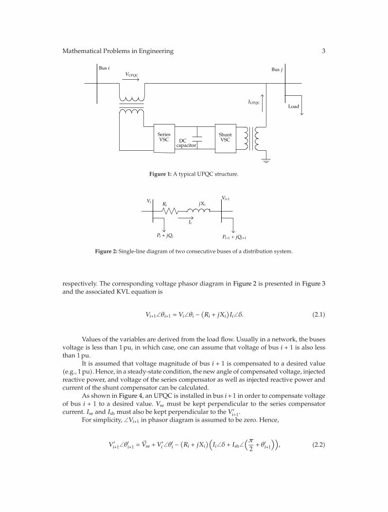
Mathematical Problems in Engineering 3
Bus i Bus jVUPQC
IUPQCLoad
SeriesVSC VSCDC
capacitor
Shunt
Figure 1: A typical UPQC structure.
Vi Ri jXi
Vi+1
Pi + jQi
Ii
Pi+1 + jQi+1
Figure 2: Single-line diagram of two consecutive buses of a distribution system.
respectively. The corresponding voltage phasor diagram in Figure 2 is presented in Figure 3and the associated KVL equation is
Vi+1∠θi+1 = Vi∠θi −(Ri + jXi
)Ii∠δ. (2.1)
Values of the variables are derived from the load flow. Usually in a network, the busesvoltage is less than 1pu, in which case, one can assume that voltage of bus i + 1 is also lessthan 1pu.
It is assumed that voltage magnitude of bus i + 1 is compensated to a desired value(e.g., 1 pu). Hence, in a steady-state condition, the new angle of compensated voltage, injectedreactive power, and voltage of the series compensator as well as injected reactive power andcurrent of the shunt compensator can be calculated.
As shown in Figure 4, an UPQC is installed in bus i+ 1 in order to compensate voltageof bus i + 1 to a desired value. Vse must be kept perpendicular to the series compensatorcurrent. Ise and Ish must also be kept perpendicular to the V ′
i+1.For simplicity, ∠Vi+1 in phasor diagram is assumed to be zero. Hence,
V ′i+1∠θ′
i+1 = �Vse + V ′i ∠θ′
i −(Ri + jXi
)(Ii∠δ + Ish∠
(π2+ θ′
i+1
)), (2.2)
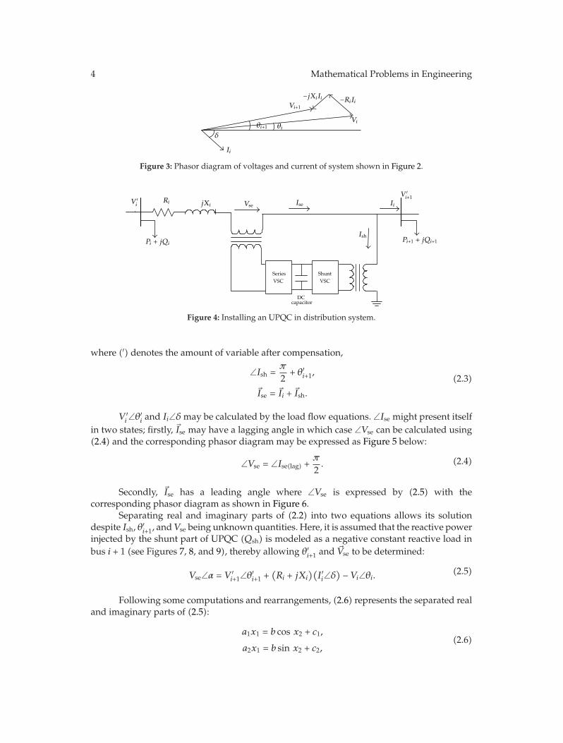
4 Mathematical Problems in Engineering
δ
Ii
θi+1 θi
Vi+1
−jXiIi −RiIi
Vi
Figure 3: Phasor diagram of voltages and current of system shown in Figure 2.
Series ShuntVSC VSC
DCcapacitor
V ′i
Ri jXi Vse Ise
Pi + jQi
Ii
V ′i+1
IshPi+1 + jQi+1
Figure 4: Installing an UPQC in distribution system.
where (′) denotes the amount of variable after compensation,
∠Ish =π
2+ θ′
i+1,
�Ise = �Ii + �Ish.
(2.3)
V ′i ∠θ′
i and Ii∠δ may be calculated by the load flow equations. ∠Ise might present itselfin two states; firstly, �Ise may have a lagging angle in which case ∠Vse can be calculated using(2.4) and the corresponding phasor diagram may be expressed as Figure 5 below:
∠Vse = ∠Ise(lag) +π
2. (2.4)
Secondly, �Ise has a leading angle where ∠Vse is expressed by (2.5) with thecorresponding phasor diagram as shown in Figure 6.
Separating real and imaginary parts of (2.2) into two equations allows its solutiondespite Ish, θ′
i+1, and Vse being unknown quantities. Here, it is assumed that the reactive powerinjected by the shunt part of UPQC (Qsh) is modeled as a negative constant reactive load inbus i + 1 (see Figures 7, 8, and 9), thereby allowing θ′i+1 and �Vse to be determined:
Vse∠α = V ′i+1∠θ′
i+1 +(Ri + jXi
)(I ′i∠δ
) − Vi∠θi.(2.5)
Following some computations and rearrangements, (2.6) represents the separated realand imaginary parts of (2.5):
a1x1 = b cos x2 + c1,
a2x1 = b sin x2 + c2,(2.6)

Mathematical Problems in Engineering 5
Ish
VseVse
δ
Ise
Ii
θ′i+1 θi+1
−jX Ii sh
Vi
Vi
+1
−jX Ii i −RiIi
V ′i+1
−RIi sh
Figure 5: Phasor diagram of voltage and current of system shown in Figure 4 in lagging mode of Ise.
Vse
Vi
Vi
+1−jX Ii i
−RiIi
V ′i+1
Ish
Ise
Vse Ii
θ′i+1
θi+1
−RIi sh
−jX Ii sh
Figure 6: Phasor diagram of voltage and current of system shown in Figure 4 in leading mode of Ise.
where
a1 = cos ρ, a2 = sin ρ, b = V ′i+1, (2.7)
c1 = real((Ri + jXi
)(Ii new∠β
)) − real(Vi∠θi), (2.8)
c2 = imag((Ri + jXi
)(Ii new∠β
)) − imag(Vi∠θi), (2.9)
x1 = Vse, x2 = θ′i+1, (2.10)
x1 =−B ±
√Δ
2A, Δ = B2 − 4AC, (2.11)
x2 = cos−1(a1x1 − c1
b
)= sin−1
(a2x1 − c2
b
). (2.12)
Here, A,B, and C are defined as
A =a21 + a2
2
b2, B = −2a1c1 + a2c2
b2, C =
c21 + c22b2
. (2.13)
As can be seen from (2.11), two roots might be assigned for the variable x1, and there-fore, two values can be obtained for θ′i+1. In order to verify the correct answers, the followingcorresponding boundary conditions need to be examined:
b = V ′i+1 = Vi+1 −→ Vse = 0. (2.14)

6 Mathematical Problems in Engineering
jXi
ViVi+1IseVse
Ri
Pi + jQi
I ′i
SeriesVSC
DCcapacitor
Pi+1 + jQi+1 − jQshjjQjQQ−− jjQjQshQ hhjj
Figure 7: Installing an UPQC in a distribution system by modeling shunt compensator as constant reactiveload.
V ′i
Vi
+1
VseVse
θ′i+1
Ise = I ′i
α
βθi+1 new
Vi+1 new −jXiI′i
−RiI′i
Figure 8: Phasor diagram of voltage and current of system that shown in Figure 7 in lagging mode of Ise.
Vi
V ′i+1
Vse
Vse
Ise = I ′i
α
β
θ′i+1
θi+1 new
Vi+1 new
−jXiI′i
−RiI′i
Figure 9: Phasor diagram of voltage and current of system shown in Figure 7 in leading mode of Ise.
x1 = (−B +√Δ)/2A is found to be the correct answer in (2.11). Hence, the reactive
power injected to the network by the series part of UPQC (Qse) for voltage correction of theconnected bus to V ′
i+1, may be expressed as
jQse = �Vse · �I∗i . (2.15)
When Qse is greater than its maximum limit (Qsemax), it can be derived by Qsemax .However, voltage magnitude of the compensated bus cannot be regulated in the
desired value. Thus, a new voltage magnitude (V ′i+1 new) and a new phase angle (θ′
i+1 new) ofcompensated bus may be expressed as
V ′i+1max
∠θ′i+1max
= Vi∠θi −((Ri + jXi
)Iinew∠β
)+ Vsemax∠α. (2.16)
2.3. Installing Model in Load Flow
In order to evaluate load flow at steady-state conditions, in the presence of UPQC in a loadflow, voltagemagnitude of the compensated bus (i+1) can be assumed to be any desired value

Mathematical Problems in Engineering 7
(with any iteration in the forward sweep), and therefore, the amount of injected reactivepower by shunt part of UPQC, (Qsh) may be modeled as a negative constant load. At thisstage, the phase angle of the compensated voltage and amount of injected reactive powerproduced by Qse can be calculated using the above equations [21].
The boundary value of Qse should be examined. In case it was greater than maximumrating limit, magnitude and phase angle of the compensated bus are calculated using(2.16), having Qse set to its maximum rating. Now new magnitude and phase angle of thecompensated bus are used to determine voltages for buses located downstream to the com-pensated bus. At this stage, new updated voltages of buses and Qsh can be used to calculateload currents in the backward sweep. This procedure is repeated until load flow convergencereaches the desired tolerance.
3. Problem Formulation
In this study, optimal location and sizing of UPQC in a steady state condition are obtainedto improve power quality. Hence, minimizing UPQC size and power loss in the distributionnetwork, is considered as the objective function (OF). The voltage and current constraints areformulated as a penalty function to the OF.
3.1. Objective Function
Equation (3.1) illustrates mathematically the proposed OF as below:
OF =
[
Ke
3∑
i=1
(Ti × Plossi) +3∑
i=1
(Kci × CostUPQCyeari
)]
×⎡
⎣3∏
i=1
∣∣∣∣∣∣
⎛
⎝nl∏
j=1
OC ×nb∏
j=1
OV
⎞
⎠
i
∣∣∣∣∣∣
⎤
⎦, (3.1)
where i, nb, and nl indicate numbers of load level, bus, and lines, respectively; Ke is theenergy cost of losses, Ti is the time duration of ith load level, and Kci is the time durationproportion of ith load level to the total time duration [31], determined as
Kci =Ti
∑3i=1 Ti
. (3.2)
Plossi is the total power loss in the ith load level, described [32] as
Plossi =nl∑
j=1
Rj
∣∣Ij∣∣2. (3.3)
The first term in the OF equation above corresponds to the total costs (in US $) of power lossand UPQC installation which should be minimized. The second term deals with the voltagesand currents limitations of network which is an important factor to be bonded within thedesired limits. This term acts as a penalty factor and is assigned in a constant ratio to the firstterm, in response to the deviation from specific boundary conditions, and equals to 1 whenall limitations are secured for buses voltages and lines currents.

8 Mathematical Problems in Engineering
3.2. Cost of UPQC
The cost of UPQC is assumed to be the same as the cost of UPFC as reported by Siemensdatabase. Cost of investment can be determined from UPQC cost [33–35] as
CostUPQC(US($/kVAr)) = 0.0003S2 − 0.2691S + 188.22,
CostUPQCyeari= CostUPQCi
(1 + B)nUPQC × B
(1 + B)nUPQC − 1.
(3.4)
In the above equations, S is the operating range of the UPQC inMVAr, CostUPQCiis the
investment cost for the ith load level in the year of allocation, CostUPQCyearicorresponds to the
annual cost of UPQC for the same load level, nUPQC is the longevity of UPQC, and B is theasset rate of return.
Minimizing the deviation of node’s voltage and line’s current is formulated in thesecond term of OF. OC and OV denote line over current factor and voltage stability index,respectively, and are defined [36] as
OC =
⎧⎪⎨
⎪⎩
1; if Ij ≤ Imax,
exp(λ
∣∣∣∣1 −Ij
Imax
∣∣∣∣
); if Ij > Imax,
OV=
{1; if Vmin ≤ Vb ≤ Vmax,
exp(μ|1 − Vb|
); otherwise.
(3.5)
Here, Ij is the current magnitude flow for the jth line, Imax is the maximum current thatcan flow in the network lines, λ and μ are small positive constants, and Vb is the voltagemagnitude for the bth bus. If all line currents are less than Imax, OCwill be equal to 1, and if allbuses voltages are within the desired boundaries, OV would equal unity; in all otherconditions, OC or OV will acquire a value (greater than 1) representing the penalty factorin OF.
Total cost saving (TCS) is the difference between total energy loss cost before installa-tion, and the sum of annual cost of UPQC and total energy loss cost after installation in thethree load levels (light, medium, and peak) considered here and may be expressed as
TCS = Ke
3∑
i=1
Ti · Plossi −Ke
3∑
i=1
Ti · PWith UPQClossi
−3∑
i=1
Kci · CostUPQCyeari. (3.6)
4. Differential Evolution Algorithm
Amongst the best known direct search approaches for nonlinear, nondifferentiable objectivefunction, introduced so far, differential evolution (DE) has proved to be an effective algo-rithm. Inherently parallel search techniques like genetic algorithms and evolution strategieshave some built-in safeguards to forestall misconvergence [37]. DE algorithm is a stochastic,population-based optimization algorithm introduced by Storn and Price in 1997 [38]. It cre-ates new candidates solutions by combining the parent individual and several other individ-uals of the same population. DE generates new vectors of parameter by adding the weighted

Mathematical Problems in Engineering 9
difference between two population vectors to a third one [39]. A candidate replaces theparent only if it has better fitness value [40]. DE is an effective, fast, simple, robust, inherentlyparallel, and has few control parameters need little tuning. It can be used tominimize noncon-tinuous, nonlinear, and nondifferentiable space function, also it can work with noisy, flat,multidimensional, and time-dependent objective functions and constraint optimization inconjunction with penalty functions [39].
The main differences between genetic algorithm (GA), immune algorithm (IA) [41],and DE are the selection process and the mutation that makes DE self-adaptive [42]. A prac-tical optimization technique is expected to fulfill three requirements: regardless of the initialsystem parameter values, the method should find the true global minimum; it shouldconverge rapidly; should be easy to use, that is, it should possess limited number of controlparameters [43–46]. The initial population of a DE algorithm is randomly generated withinthe control variable bounds. This population is successfully improved over generations byapplying mutation, crossover and selection operators, to reach an optimal solution. The sizeof population, however, is constant during the process. At the end of each generation, the bestindividuals based on his OF value are stored. In short, DE operation includes four stages[24, 43–46] as described below.
4.1. Population Initialization
Initial population is a number of parameter vectors (PVs), randomly generatedwithin the tar-get parameters’ limits. For the Gth generation, the population containsNp multidimensionalPVs xi,G = [x1
i,G, x2i,G, . . . , x
Di,G], where i represents the number of the PV. The kth parameter in
the ith PV of the first generation can be obtained by (4.1):
xki,1 = xk
min + rand(0, 1) ×(xkmax − xk
min
)i ∈ [
1,Np
], k ∈ [1, D], (4.1)
where xkmin and xk
max are the lower and upper bounds of the kth parameter, respectively, andrand (0, 1) is a random scalar within [0, 1] as shown in Figure 10. In case there is a prioriknowledge available about the problem, the preliminary solution may be included to theinitial population by adding normally distributed random deviations to the nominal solution[47].
4.2. Mutation
DE does not use a predefined probability density function to generate perturbing fluctua-tions. It relies upon the population itself to perturb the vector parameter [48]. For eachmember i from the population, DE generates a mutated PV, vi,G+1, by adding the weighteddifference of two randomly selected PVs to a third randomly selected PV as
vi,G+1 = xr3,G + s(xr1,G − xr2,G), (4.2)
where the subscripts r1, r2, and r3 represent the randomly selected PVs such that r1 /= r2 /= r3 /= i.s is a user-defined constant called the step size. It controls the scale of differential variationand usually selected to be in the range of 0 ≤ s ≤ 2. The corresponding objective function will

10 Mathematical Problems in Engineering
xGr1− xG
r2
xGr3+ F(xG
r1− xG
r2)
F(xGr1− xG
r2)xG
r2
xGr1
xGr3
xGi
0 0.5 1 1.5 2 2.5 3 3.5 4
0
0.5
1
1.5
2
2.5
: parameter vectors in current population (G)
x2
x1
min.
Contour
Figure 10: Two-dimensional example of DE method (creation of new generation from current generation).
be compared with a predetermined individual PV. Note that if any parameter of the mutatedPV, vi,g , is found outside the related boundaries, it will be fixed at the corresponding upperor lower limits. This ensures that the best parameter vector is evaluated for every generationin order to track the progress made throughout the minimization process.
4.3. Crossover Operation
The main idea behind DE is a scheme for generating trial PVs. When faced with smallpopulation diversity, the population could rapidly cluster together leading to prematureconvergence and restricted improvement. In such circumstances, in order to increase thelocal diversity of the mutant populations, a crossover is introduced [48]. For this purpose,parameters of the mutated PV, vi,G+1, are mixed with the so-called target PV, xi,G, in order toform the trial PV, ui,G+1 as below
uki,G+1 =
{vki if randk
i ≤ CR or k = Jrand,
xki,G if randk
i > CR and k /= Jrand,(4.3)
where the superscript k indicates that the kth component of the trial PV, randki is a random
scalar so that 0 ≤ randki ≤ 1, and Jrand is a randomly chosen integer so that 1 ≤ Jrand ≤ D. Jrand
is chosen once for each vector and ensures that ui,G+1 obtains at least one parameter fromvi,G+1. CR, the DE controlling parameter, is called crossover rate which is user-defined andusually within the range 0 < CR < 1.
4.4. Evaluation and Selection
After generating the trial PV, ui,G+1, if the obtained cost function is lower than the target PV,xi,G, then xi,G+1 will be set to ui,G+1; otherwise xi,G will be retained. To complete an iteration,

Mathematical Problems in Engineering 11
Start
Initialize the vectors of candidate solutions of the parent population
Run load flow and calculation of objective function
Mutation and crossover of control variables to generate a trial vector
Run load flow and calculation of new solution objective function
Selection operation
Convergence orGen i >max gen
Print best vector of population with min. OF
End
i
N
= i + 1
Figure 11: Flowchart of DE algorithm.
each PV of the population has to serve once as the target PV. All members of populationwith similar opportunity can be selected as parents. If parents have a better OF, they will beretained. The best of these are selected to reconstruct the new generation.
The procedure comes to a halt when an acceptable solution candidate is reached or noimprovement in new generations is accrued or the number of iterations exceeds its limit. InFigure 11, a flowchart of DE algorithm is presented.
5. Implementation of DE for Finding Optimal Location andSize of UPQC
As mentioned before, DE algorithm is applied to search the best location and size of UPQCin network for each load level, such that OF becomes minimum, that means minimum powerloss, size and cost of UPQC, and deviation of voltages/currents from the desired values.
Two case studies are presented in this section, including a 33-bus and 69-bus standardIEEE distribution network that work at 12.66 kV and have radial structure [49, 50]. Thesedistribution networks are shown in Figures 12 and 13, respectively.

12 Mathematical Problems in Engineering
1 2
19 20 21 22
3 4 5 6 7 8 9 10 11 12 13 14 15 16 17 18
26
23 24 25
27 28 29 30 31 32 33
Figure 12: Single-line diagram of IEEE 33-bus distribution system.
36
47 48 49 50
51 52 68 69
37 38 39 40 41 42 43 44 45 46
1 2 3 4 5 6 7 8 9 10
66 67
53 54 55 56 57 58 59 60 61 62 63 64 65
28 29 30 31 32 33 34 35
11 12 13 14 15 16 17 18 19 20 21 22 23 24 25 26 27
Figure 13: Single-line diagram of IEEE 69-bus distribution system.
In order to model the annual load profile, three load levels are selected including light,medium, and peak. Table 1 shows the time duration and total load for each load level in twotest systems.
In order to evaluate the effectiveness of DE, its performance is compared with GA andIA, run on the same basis. To find the optimum set of parameters for DE, GA, and IA, 50 trialsare performed for each possible set of parameters. For each trial the optimum OF is recorded,and the appropriate statistical measures are compared in the following.
Maximum iteration and initial population sizes are set to 100 and 50, respectively.Initial binary strings (chromosomes) are randomly produced, containing a number ofselected bus for compensation as well as three values for voltages of compensated node inthree load levels. The corresponding DE, GA, and IA settings are shown in Table 2.
After running the load flow in three load levels, OF is calculated for each chromosome.The OF parameters applied are indicated in Table 3 [50–53].
It should be noted that the constraint ofQUPQC, voltages of buses, and currents of lines(for Lynx conductor [54] at 30◦C) are as indicated below:
0 ≤ QUPQCkVAr ≤ 10000kVAr,
0.9 ≤ Vpu. ≤ 1.1,
IMax ≤ 520A.
(5.1)

Mathematical Problems in Engineering 13
Table 1: Load level and load duration time in 33- and 69-bus IEEE test systems.
Load level Light Medium PeakTime duration (h) 2000 5260 1500
Total load (kVAr) 33 buses 3715 + j2300 4829.5 + j2300 5944 + j230069 buses 3802.2 + j2694.6 4942.8 + j2694.6 6083.5 + j2694.6
Total power loss (kW) 33 buses 202.68 305.86 442.4169 buses 225.00 342.99 502.52
Table 2: Parameters setting of the DE, GA, and IA methods.
S CR Mutation rate Selection rate Pr Pc Pm
DE 0.7 1 — — — — —GA — — 0.3 0.5 — — —IA — — — — 0.3 0.9 0.1
Table 3: OF parameters setting for optimization.
nUPQC (year) B Ke US ($/kWhr) λ μ Kci
30 0.1 0.06 2 1Load Level (i)
1 2 30.22831 0.60046 0.17123
6. Simulation Results
The effectiveness of proposed approach is illustrated using IEEE 33-bus and IEEE 69-bussystems. It is tried to obtain the optimal solution using the OF given by (3.1) in two samplenetworks; the simulation results are described in the following sections.
6.1. IEEE 33-Bus Test System
Table 4 shows the placement and size of UPQC, and also the minimumOF using GA, IA, andDE methods in IEEE 33-bus distribution system in three load levels.
Compared with GA and IA, DE seems to offer an improved optimal solution with itslower OF. In this system, the 29th bus is selected for UPQC installation by DE and 33th and28th bus are selected by GA and IA methods for compensating for light, medium, and peakload levels, respectively.
Although IA has managed to find installation location fairly close to that of the DE,it has performed weaker in finding the best size of UPQC in the three load levels. Locationcandidates have a discrete search space, while search space for size of UPQC is wide andcontinuous causingmore difficult search for the IAmethod compared with DE. In this regard,GA does not seem to present any suitable result for both location and size as compared withDE. By increasing the load level, all algorithms suggest reasonably greater size of UPQC(with greater shunt size compared with series size). Table 5 presents comparison of powerloss, annual cost of UPQC, number of under voltage buses, and number of over current linesbefore and after installation using DE algorithm in the three load levels, in the IEEE 33-busdistribution system.

14 Mathematical Problems in Engineering
Table 4: Comparison results of OF value, optimal location, and sizing of UPQC in IEEE 33-bus test system.
OFDE 158784.1GA 186510.3IA 165598.1
LocationDE 29GA 33IA 28
Light Medium Peak
Size (kVAr)
DE Shunt 914.1 1158.1 2457.3Series 0.0015 39.6 125.9
GA Shunt 917 1574 2953.9Series 3.65 17.65 50.9
IA Shunt 508.1 910.6 1502Series 0.902 20.1 76.46
Table 5: Summary results of IEEE 33-bus distribution system.
Load level Light Medium Peak
Total power loss (kW)∗B I 202.68 305.86 442.41∗∗A I 150.3 244.44 402.7
CostUPQCyear ($) A I 18254 23912 51575
Number of under voltage buses B I 0 7 14A I 0 0 0
Number of over current lines B I 0 0 2A I 0 0 0
∗Before installation.∗∗After installation.
Table 6: Comparison of annual costs of IEEE 33-bus test system.
Total energy loss cost BI ($) 1.6067∗105
Total energy loss cost AI ($) 1.3143∗105
Total annual cost of UPQC ($) 2.7357∗104
Total cost saving ($) 1.8829∗103
Table 7: CPU time for optimization in IEEE 33-bus test system.
Algorithm DE GA IACPU time (second) 5512 9053 8102
Results indicate a power loss reduction in all three load levels, and in general, the totalpower loss is reduced by 18.2%, while all voltages and currents are within the desired limits.In the third load level, total power loss is decreased by 8.9% because size reduction of UPQChas led to buses voltages to go out of the desired boundaries and increased size of UPQChas led to increased power loss. Hence, this solution is an optimum point to supply bothboundaries.
Table 6 presents the annual results of economic evaluations. As can be seen, total costsaving will be 1885.9 $.
Mathematical Problems in Engineering 15
Table 8: Comparison results of OF value, optimal location, and sizing of UPQC in IEEE 69-bus test system.
DE 170181.9OF GA 220877.4
IA 181761.2DE 62
Location GA 58IA 60
Light Medium Peak
Series size (kVAr)
DE Shunt 1089.7 1156.2 2240.2Series 11.3 73.8 280.6
GA Shunt 1200.3 1431 2290.3Series 24 111 312.1
IA Shunt 1092.8 1187.1 2235.9Series 32.6 71 300
Table 9: Summary results of IEEE 69-bus distribution system.
Load level Light Medium Peak
Total power loss (kW) B I 225 343 502.5A I 155.1 265.7 437.1
CostUPQC year ($) A I 21948 23115 50150
Number of under voltage buses B I 0 6 8A I 0 0 0
Number of over current lines B I 0 0 4A I 0 0 0
Table 10: Comparison of annual costs of IEEE 69-bus test system.
Total energy loss cost BI ($) 1.8047∗105
Total energy loss cost AI ($) 1.4180∗105
Total annual cost of UPQC ($) 2.8383∗104
Total cost saving ($) 1.0288∗104
Table 11: CPU time for optimization in IEEE 69-bus test system.
Algorithm DE GA IACPU time (second) 8137 13137 11433
The proposed method has been implemented on a quad computer with 2.8GHZ CPU.Table 7 shows CPU time for each algorithm, indicating a much faster convergence by DE thanGA and IA.
Figure 14 shows voltages of buses before and after UPQC installation using DEalgorithm in each load level in the IEEE 33-bus distribution network. Results shows improvement in voltage profiles after installation UPQC in each load level. Location of UPQC isindicated by the arrow.
The convergence curves for the OF obtained by DE, IA, and GA are represented inFigure 15. Results show that DE has a faster convergence and better ability in searching the

16 Mathematical Problems in Engineering
0.8
0.85
0.9
0.95
1
1.05
1 3 5 7 9 11 13 15 17 19 21 23 25 27 29 31 33V
olta
ge (P
u)
Bus number
Light BI
Light AIMedium BIMedium AIHeavy BI
Heavy AI
Figure 14: Voltages for the 33-bus distribution network before and after UPQC installation.
minimumOF compared with both IA and GAmethods. DE is converged at the 44th iteration,while IA and GA have done so at the 53th and 65th iterations, respectively.
6.2. IEEE 69-Bus Test System
Table 8 shows placement and size of the UPQC as well as the minimum OF using DE, GA,and IA methods in the IEEE 69-bus system in the three load levels.
Similarly, DE offers better optimal solution here (i.e., lower OF and lower UPQCsize) compared to GA and IA. In this 69-bus case study, the 62th bus is selected for UPQCinstallation by DE and the 58th and 60th buses are selected for UPQC installation by GA andIA methods, respectively, in the three load levels. Table 9 shows the similar results to thoseof Table 5, but for the 69-bus distribution system. Minimum voltage and maximum currentof the system have improved and the system losses are reduced in each load level. Generally,total power loss was reduced by 21.42%.
Annual results of economic evaluation for the 69-bus system are presented in Table 10with total cost saving of 10288 $. Table 11 shows CPU time for each algorithm. The same as33 bus system, here, DE has a faster convergence and better optimal solution than both GAand IA.
Figure 16 shows voltages of buses before and after installation UPQC using DEalgorithm in each load level for IEEE 69-bus distribution network. In this figure, improvementin voltage profile is evident. Location of UPQC is again represented by the arrow. Figure 17shows the convergence diagram for DE, IA, and GA. Results show that DE has faster con-vergence compared with IA and GA so that DE converged at the 23th iteration, while IA andGA do it at the 55th and 65th iterations, respectively. Best candidate of DE has the lowest OFamong the three algorithms indicating superior searching ability of DE algorithm. As before,IA has a close UPQC location to DE because of limited and discrete searching space, but asfor searching the best size of the UPQC, it has performed weaker compare to the DE. GA toohas performed weaker in both finding the location and size of UPQC compared to DE andIA.

Mathematical Problems in Engineering 17
0 10 20 30 40 50 60 70 80 90 10002468
1012141618
Number of iteration
OF
DEIAGA
70 75 80 85 90 95 1001.51.61.71.81.9
×105
×105
Figure 15: Convergence diagram of DE, IA, and GA methods.
0.75
0.8
0.85
0.9
0.95
1
1.05
1 5 9 13 17 21 25 29 33 37 41 45 49 53 57 61 65 69
Vol
tage
(Pu)
Bus number
Light BILight AIMedium BI
Medium AIHeavy BIHeavy AI
Figure 16: Voltages of the 69-bus distribution network before and after UPQC installation.
0 10 20 30 40 50 60 70 80 90 1000
1
2
3
4
5
6
7
8
Number of iteration
OF
70 75 80 85 90 95 1001.6
1.8
2
2.2
2.4
DEGAIA
×108
×105
Figure 17: Convergence diagram of DE, IA, and GA methods.

18 Mathematical Problems in Engineering
7. Conclusion
A new approach is proposed in this paper for the discrete optimization problem of UPQCplacement and sizing in radial distribution systems using DE method. The DE method forminimizing continuous space functions has been introduced and shown to be superior to GAand IAmethods. Energy and power losses due to installed UPQC as well as its associated costare used to define the OF. For system solution, backward/forward sweep load flow is applied.Simulation results indicate that OF reduction may be obtained utilizing UPQC. Using DEmethod, the optimal location and size of UPQC is obtained in order to decrease power loss,cost of UPQC and current profile, and improve voltage. Compared with IA and GA, DEconverges faster and smoother. Compared with GA and IA, DE technique provides minimumUPQC size, CPU time, and OF. Installation of the UPQC by the proposed approach leads to18.2% and 21.42% power loss reductions, in 33- and 69-bus distribution systems, respectively.All bus voltages and currents of lines are within the desired boundaries. Reduction in totalenergy loss cost are 18.198% and 21.427% in 33- and 69-bus distribution network, respectively.Total cost saving as a result of this exercise is estimated to be of the order of 1.2% and 5.7% inthe 33- and 69-bus IEEE test systems, respectively.
References
[1] A. Ghosh and G. Ledwich, “A unified power quality conditioner (UPQC) for simultaneous voltageand current compensation,” Electric Power Systems Research, vol. 59, no. 1, pp. 55–63, 2001.
[2] R. C. Dugan, M. F. McGranaghan, and H.W. Beaty, Electrical Power System Quality, McGrawHill, NewYork, NY, USA, 1996.
[3] E. Acha, V. G. Agelidis, O. Anaya-Lara, and T. J. E. Miller, Power Electronic Control in Electrical Systems,Newnes, Melbourne, Australia, 2002.
[4] A. Ghosh and G. Ledwich, “Compensation of distribution system voltage using DVR,” IEEETransactions on Power Delivery, vol. 17, no. 4, pp. 1030–1036, 2002.
[5] X. P. Zhang, “Advanced modeling of the multi-control functional static synchronous series compen-sator (SSSC) in Newton power flow,” IEEE Transactions on Power Systems, vol. 18, no. 4, pp. 1410–1416,2003.
[6] G. Chen, Y. Chen, L. F. Sanchez, and K. M. Smedley, “Unified power quality conditioner fordistribution system without reference calculations,” in Proceedings of the 4th International PowerElectronics and Motion Control Conference (IPEMC ’04), vol. 3, pp. 1201–1206, August 2004.
[7] A. K. Jindal, A. Ghosh, and A. Joshi, “Interline unified power quality conditioner,” IEEE Transactionson Power Delivery, vol. 22, no. 1, pp. 364–372, 2007.
[8] H. Fujita and H. Akagi, “The unified power quality conditioner: the integration of series- and shunt-active filters,” IEEE Transactions on Power Electronics, vol. 13, no. 2, pp. 315–322, 1998.
[9] F. Kamran and T. G. Habetler, “Combined deadbeat control of a series-parallel converter combinationused as a universal power filter,” IEEE Transactions on Power Electronics, vol. 13, no. 1, pp. 160–168,1998.
[10] P. T. Nguyen and T. K. Saha, “Dynamic voltage restorer against balanced and unbalanced voltagesags: modelling and simulation,” in Proceedings of the IEEE Power Engineering Society General Meeting,vol. 1, pp. 639–644, June 2004.
[11] M. Chawla, A. Rajvanshy, A. Ghosh, and A. Joshi, “Distribution bus voltage control using DVR underthe supply frequency variations,” in Proceedings of the IEEE Power India Conference, pp. 25–30, April2006.
[12] M.Hu andH. Chen, “Modeling and controlling of unified power quality compensator,” in Proceedingsof the IEEE International Conference on Advances in Power System Control, Operation and Management, vol.2, pp. 431–435, October 2000.
[13] Y. Y. Kolhatkar, R. R. Errabelli, and S. P. Das, “A sliding mode controller based optimum UPQC withminimum VA loading,” in Proceedings of the IEEE Power Engineering Society General Meeting, pp. 2240–2244, June 2005.
Mathematical Problems in Engineering 19
[14] M. Basu, S. P. Das, and G. K. Dubey, “Performance study of UPQC-Q for load compensation andvoltage sag mitigation,” in Proceedings of the 28th Annual Conference of the IEEE Industrial ElectronicsSociety, pp. 698–703, November 2002.
[15] F. Z. Peng, H. Akagi, andA.Nabae, “A new approach to harmonic compensation in power systems—acombined system of shunt passive and series active filters,” IEEE Transactions on Industry Applications,vol. 26, no. 6, pp. 983–990, 1990.
[16] F. Silva, “Control methods for power converters,” in Handbook of Power Electronics, M. H. Rashid, Ed.,2002.
[17] T. S. Key and J. S. Lai, “Comparison of standards and power supply design options for limitingharmonic distortion in power systems,” IEEE Transactions on Industry Applications, vol. 29, no. 4, pp.683–695, 1993.
[18] B. Han, B. Bae, H. Kim, and S. Baek, “Combined operation of unified power-quality conditioner withdistributed generation,” IEEE Transactions on Power Delivery, vol. 21, no. 1, pp. 330–338, 2006.
[19] G. Jianjun, X. Dianguo, L. Hankui, and G. G. Maozhong, “Unified power quality conditioner (UPQC):the principle, control and application,” in Proceedings of the Power Conversion Conference, vol. 1, pp. 80–85, 2002.
[20] C. Yunping, Z. Xiaoming, W. Jin, L. Huijin, S. Jianjun, and T. Honghai, “Unified power qualityconditioner (UPQC): the theory, modeling and application,” in Proceedings of the IEEE InternationalConference on Power System Technology, vol. 3, pp. 1329–1333, 2000.
[21] M. Hosseini, H. A. Shayanfar, and M. Fotuhi-Firuzabad, “Modeling of unified power qualityconditioner (UPQC) in distribution systems load flow,” Energy Conversion and Management, vol. 50,no. 6, pp. 1578–1585, 2009.
[22] V. Khadkikar, A. Chandra, A. O. Barry, and T. D. Nguyen, “Steady state power flow analysis ofunified power quality conditioner (UPQC),” in Proceedings of the International Conference on IndustrialElectronics and Control Applications (ICIECA ’05), pp. 6–16, December 2005.
[23] R. Storn andK. Price, “Minimizing the real functions of the ICEC ’96 contest by differential evolution,”in Proceedings of the IEEE International Conference on Evolutionary Computation (ICEC ’96), pp. 842–844,May 1996.
[24] R. Storn and K. Price, “Differential Evolution—a simple and efficient adaptive scheme for globaloptimization over continuous spaces,” Journal of Global Optimization, vol. 11, no. TR-95-012, pp. 1–15,1997.
[25] H. Akagi, “New trends in active filters for power conditioning,” IEEE Transactions on Industry Applica-tions, vol. 32, no. 6, pp. 1312–1322, 1996.
[26] M. Basu, S. P. Das, and G. K. Dubey, “Experimental investigation of performance of a single phaseUPQC for voltage sensitive and non-linear loads,” in Proceedings of the 4th IEEE International Conferenceon Power Electronics and Drive Systems, pp. 218–222, October 2001.
[27] R. Rajasree and S. Premalatha, “Unified power quality conditioner (UPQC) control using feed for-ward (FF)/ feed back (FB) controller,” in Proceedings of the International Conference on Computer, Com-munication and Electrical Technology (ICCCET ’11), pp. 364–369, March 2011.
[28] S. Ghosh and D. Das, “Method for load-flow solution of radial distribution networks,” IEE Proceed-ings, vol. 146, no. 6, pp. 641–648, 1999.
[29] M. Hosseini, H. A. Shayanfar, andM. Fotuhi, “Modeling of series and shunt distribution facts devicesin distribution load flow,” Journal of Electrical Systems, vol. 4, no. 4, pp. 1–12, 2008.
[30] E. Acha, C. R. Fuerte-Esquivel, H. Ambriz-Perez, and C. Angeles-Camacho, FACTS Modeling andSimulation in Power Networks, Wiley, New York, NY, USA, 2004.
[31] I. C. da Silva Jr., S. Carneiro, E. J. de Oliveira, J. de Souza Costa, J. L. Rezende Pereira, and P. A. N.Garcia, “A heuristic constructive algorithm for capacitor placement on distribution systems,” IEEETransactions on Power Systems, vol. 23, no. 4, pp. 1619–1626, 2008.
[32] D. Das, “Optimal placement of capacitors in radial distribution system using a Fuzzy-GA method,”International Journal of Electrical Power and Energy Systems, vol. 30, no. 6-7, pp. 361–367, 2008.
[33] S. A. Taher and M. K. Amooshahi, “Optimal placement of UPFC in power systems using immunealgorithm,” Simulation Modelling Practice and Theory, vol. 19, no. 5, pp. 1399–1412, 2011.
[34] S. A. Taher and A. A. Abrishami, “UPFC location and performance analysis in deregulated powersystems,”Mathematical Problems in Engineering, vol. 2009, Article ID 109501, 2009.
[35] D. Povh, “Modeling of FACTS in power system studies,” in Proceedings of the IEEE Power EngineeringSociety Winter Meeting (PES ’00), vol. 2, pp. 1435–1439, 2000.

20 Mathematical Problems in Engineering
[36] M. Saravanan, S. M. R. Slochanal, P. Venkatesh, and J. P. S. Abraham, “Application of particle swarmoptimization technique for optimal location of FACTS devices considering cost of installation andsystem loadability,” Electric Power Systems Research, vol. 77, no. 3-4, pp. 276–283, 2007.
[37] R. Storn and K. Price, “Differential evolution—a simple and efficient adaptive scheme for globaloptimization over continuous spaces,” ICSI Technical Report, no. TR-95-012, pp. 1–5, 1995.
[38] R. Storn and K. Price, “Differential evolution—a simple and efficient adaptive scheme for globaloptimization over continuous spaces,” Journal of Global Optimization, vol. 11, no. 4, pp. 341–359, 1997.
[39] H. I. Shaheen, G. I. Rashed, and S. J. Cheng, “Optimal location and parameter setting of UPFC forenhancing power system security based on differential evolution algorithm,” International Journal ofElectrical Power and Energy Systems, vol. 33, no. 1, pp. 94–105, 2011.
[40] J. M. Ramirez, J. M. Gonzalez, and T. O. Ruben, “An investigation about the impact of the optimalreactive power dispatch solved by DE,” International Journal of Electrical Power and Energy Systems, vol.33, no. 2, pp. 236–244, 2011.
[41] S. A. Taher and M. Karim Amooshahi, “New approach for optimal UPFC placement using hybridimmune algorithm in electric power systems,” International Journal of Electrical Power and EnergySystems, vol. 43, no. 1, pp. 899–909, 2012.
[42] A. A. Abou El Ela, M. A. Abido, and S. R. Spea, “Optimal power flow using differential evolutionalgorithm,” Electric Power Systems Research, vol. 80, no. 7, pp. 878–885, 2010.
[43] A. Ketabi and M. J. Navardi, “Optimization shape of variable capacitance micromotor using differen-tial evolution algorithm,”Mathematical Problems in Engineering, vol. 2010, Article ID 909240, 15 pages,2010.
[44] S. Sayah and K. Zehar, “Modified differential evolution algorithm for optimal power flow with non-smooth cost functions,” Energy Conversion and Management, vol. 49, no. 11, pp. 3036–3042, 2008.
[45] A. A. A. E. Ela, M. A. Abido, and S. R. Spea, “Differential evolution algorithm for optimal reactivepower dispatch,” Electric Power Systems Research, vol. 81, no. 2, pp. 458–464, 2011.
[46] M. Varadarajan and K. S. Swarup, “Network loss minimization with voltage security usingdifferential evolution,” Electric Power Systems Research, vol. 78, no. 5, pp. 815–823, 2008.
[47] I. Hussain and A. K. Roy, “Optimal size and location of distributed generations using differentialevolution (DE),” in Proceedings of the 2nd National Computational Intelligence and Signal Processing (CISP’12), pp. 57–61, 2012.
[48] C. Bulac, F. Ionescu, and M. Roscia, “Differential evolutionary algorithms in optimal distributedgeneration location,” in Proceedings of the 14th International Conference on Harmonics and Quality of Power(ICHQP ’10), pp. 1–5, September 2010.
[49] M. E. Baran and F. F. Wu, “Network reconfiguration in distribution systems for loss reduction andload balancing,” IEEE Transactions on Power Delivery, vol. 4, no. 2, pp. 1401–1407, 1989.
[50] N. Mithulananthan, A. Sode-yome, and N. Acharya, “Application of FACTS controllers in Thailandpower systems,” FACTS project, Chulangkorn University, Final Report, 2005.
[51] K. Vijayakumar and R. P. Kumudinidevi, “A new method for optimal location of FACTS controllersusing genetic algorithm,” Journal of Theoretical and Applied Information Technology, vol. 3, no. 4, pp. 1–6,2007.
[52] F. D. Galiana, K. Almeida, M. Toussaint et al., “Assessment and control of the impact of facts deviceson power system performance,” IEEE Transactions on Power Systems, vol. 11, no. 4, pp. 1931–1936,1996.
[53] B. A. Renz, A. Keri, A. S. Mehraban et al., “AEP unified power flow controller performance,” IEEETransactions on Power Delivery, vol. 14, no. 4, pp. 1374–1381, 1999.
[54] T. A. Short, Electric Power Distribution Handbook, CRC Press, New York, NY, USA, 2004.

Submit your manuscripts athttp://www.hindawi.com
Hindawi Publishing Corporationhttp://www.hindawi.com Volume 2014
MathematicsJournal of
Hindawi Publishing Corporationhttp://www.hindawi.com Volume 2014
Mathematical Problems in Engineering
Hindawi Publishing Corporationhttp://www.hindawi.com
Differential EquationsInternational Journal of
Volume 2014
Applied MathematicsJournal of
Hindawi Publishing Corporationhttp://www.hindawi.com Volume 2014
Probability and StatisticsHindawi Publishing Corporationhttp://www.hindawi.com Volume 2014
Journal of
Hindawi Publishing Corporationhttp://www.hindawi.com Volume 2014
Mathematical PhysicsAdvances in
Complex AnalysisJournal of
Hindawi Publishing Corporationhttp://www.hindawi.com Volume 2014
OptimizationJournal of
Hindawi Publishing Corporationhttp://www.hindawi.com Volume 2014
CombinatoricsHindawi Publishing Corporationhttp://www.hindawi.com Volume 2014
International Journal of
Hindawi Publishing Corporationhttp://www.hindawi.com Volume 2014
Operations ResearchAdvances in
Journal of
Hindawi Publishing Corporationhttp://www.hindawi.com Volume 2014
Function Spaces
Abstract and Applied AnalysisHindawi Publishing Corporationhttp://www.hindawi.com Volume 2014
International Journal of Mathematics and Mathematical Sciences
Hindawi Publishing Corporationhttp://www.hindawi.com Volume 2014
The Scientific World JournalHindawi Publishing Corporation http://www.hindawi.com Volume 2014
Hindawi Publishing Corporationhttp://www.hindawi.com Volume 2014
Algebra
Discrete Dynamics in Nature and Society
Hindawi Publishing Corporationhttp://www.hindawi.com Volume 2014
Hindawi Publishing Corporationhttp://www.hindawi.com Volume 2014
Decision SciencesAdvances in
Discrete MathematicsJournal of
Hindawi Publishing Corporationhttp://www.hindawi.com
Volume 2014
Hindawi Publishing Corporationhttp://www.hindawi.com Volume 2014
Stochastic AnalysisInternational Journal of