Optimal Location and Sizing of Dynamic VArs

for Fast Voltage Collapse

by

Ahmed Salloum

A Thesis Presented in Partial Fulfillment

of the Requirements for the Degree

Master of Science

Approved April 2011 by the

Graduate Supervisory Committee:

Vijay Vittal, Chair

Gerald Heydt

Raja Ayyanar

ARIZONA STATE UNIVERSITY

May 2011

i

ABSTRACT

Recent changes in the energy markets structure combined with the conti-

nuous load growth have caused power systems to be operated under more stressed

conditions. In addition, the nature of power systems has also grown more complex

and dynamic because of the increasing use of long inter-area tie-lines and the high

motor loads especially those comprised mainly of residential single phase A/C

motors. Therefore, delayed voltage recovery, fast voltage collapse and short term

voltage stability issues in general have obtained significant importance in relia-

bility studies. Shunt VAr injection has been used as a countermeasure for voltage

instability. However, the dynamic and fast nature of short term voltage instability

requires fast and sufficient VAr injection, and therefore dynamic VAr devices

such as Static VAr Compensators (SVCs) and STATic COMpensators (STAT-

COMs) are used. The location and size of such devices are optimized in order to

improve their efficiency and reduce initial costs. In this work time domain dy-

namic analysis was used to evaluate trajectory voltage sensitivities for each time

step. Linear programming was then performed to determine the optimal amount of

required VAr injection at each bus, using voltage sensitivities as weighting fac-

tors. Optimal VAr injection values from different operating conditions were

weighted and averaged in order to obtain a final setting of the VAr requirement.

Some buses under consideration were either assigned very small VAr injection

values, or not assigned any value at all. Therefore, the approach used in this work

was found to be useful in not only determining the optimal size of SVCs, but also

their location.

ii

TABLE OF CONTENTS

Page

LIST OF TABLES .......................................................................................................... v

LIST OF FIGURES ....................................................................................................... vi

LIST OF SYMBOLS ................................................................................................... viii

CHAPTER

1 INTRODUCTION .................................................................................................... 1

1.1 Overview ................................................................................................... 1

1.2 Literature Review ..................................................................................... 2

1.3 Thesis Organization.................................................................................. 4

2 LOAD MODELING ................................................................................................ 6

2.1 Introduction ............................................................................................... 6

2.2 Load Model Requirements ...................................................................... 8

2.3 Present Load Modeling Practices ............................................................ 9

2.3.1 Simplified voltage dependant models ........................................ 9

2.3.2 Measurement Based Modeling ................................................. 10

2.3.3 Component Based Modeling .................................................... 11

2.4 Static Composite Load Model (ZIP) ..................................................... 13

2.5 Motor Modeling...................................................................................... 14

2.5.1 Induction Motor Modeling ....................................................... 17

2.5.2 Single Phase A/C Motor ........................................................... 18

2.5.3 Single phase A/C motor modeling ........................................... 20

iii

CHAPTER Page

2.6 Composite load model structure ............................................................ 20

3 VOLTAGE STABILITY AND VAR COMPENSATION................................. 23

3.1 Introduction ............................................................................................. 23

3.2 Classification of Voltage Stability ........................................................ 25

3.3 Voltage Stability Analysis ..................................................................... 26

3.3.1 Static Analysis .......................................................................... 27

3.3.2 Nonlinear Dynamic Analysis ................................................... 30

3.4 Reactive Power Support Measures ....................................................... 31

3.4.1 Synchronous Condensers ......................................................... 32

3.4.2 Series Capacitors ...................................................................... 33

3.4.3 Shunt Capacitor Banks ............................................................. 34

3.4.4 Shunt Reactors .......................................................................... 35

3.4.5 Static VAr Systems .................................................................. 35

4 PROPOSED METHODOLOGY .......................................................................... 40

4.1 Motivation ............................................................................................... 40

4.2 Objective ................................................................................................. 40

4.3 Static Analysis ........................................................................................ 41

4.4 Dynamic Models .................................................................................... 41

4.5 Trajectory Sensitivity Index .................................................................. 42

4.6 Linear Programming .............................................................................. 43

4.7 Generalizing Results .............................................................................. 46

iv

CHAPTER Page

5 STUDY RESULTS ................................................................................................ 49

5.1 System Representation ........................................................................... 49

5.2 Base Contingency Selection .................................................................. 49

5.3 Dynamic Load Modeling ....................................................................... 53

5.4 Trajectory Voltage Sensitivity Results (base case) .............................. 57

5.5 Optimization Results (base case) .......................................................... 58

5.5.1 Non-weighted Results .............................................................. 59

5.5.2 Weighted Results ...................................................................... 61

5.6 The Relation Between Voltage Trajectory Sensitivity and Optimal

VAr Injection ....................................................................................................... 64

5.7 Different Operating Conditions Results ............................................... 67

5.8 A Description of Contingency Results ................................................. 74

6 CONCLUSIONS AND FUTURE RESEARCH ................................................. 81

6.1 Conclusions ............................................................................................. 81

6.2 Future work ............................................................................................. 82

REFERENCES ............................................................................................................. 84

v

LIST OF TABLES

Table Page

5.1 System components ..................................................................................... 49

5.2 Representative load buses ............................................................................ 51

5.3 TSIj for VAr injection buses ........................................................................ 58

5.4 Optimized, non-weighted VAr injection values (base case) ........................ 59

5.5 Optimized, weighted VAr injection values (base case) ............................... 62

5.6 Bus trajectory sensitivity indices and corresponding optimal

VAr injection ........................................................................................................ 65

5.7 Bus trajectory sensitivity indices for different operating conditions ........... 68

5.8 Optimized weighted VAr injection values for different operating

conditions .............................................................................................................. 69

5.9 Final optimized VAr injection values .......................................................... 70

vi

LIST OF FIGURES

Figure Page

2.1 Component based modeling ......................................................................... 12

2.2 Induction motor torque and current curves .................................................. 16

2.3 Single cage rotor IM equivalent circuit ....................................................... 17

2.4 Reactive power consumption for a stalled single phase induction

A/C motor ............................................................................................................. 19

2.5 LMTF proposed composite load model ....................................................... 22

3.1 TSC schematic representation...................................................................... 36

3.2 TCR schematic representation ..................................................................... 37

3.3 SVC and STATCOM characteristic curves ................................................. 39

5.1 Load bus voltage magnitude (static load models) set-1 ............................... 52

5.2 Load bus voltage magnitude (static load models) set-2 ............................... 53

5.3 Load bus voltage magnitude (dynamic load models) set-1 ......................... 55

5.4 Load bus voltage magnitude (dynamic load models) set-2 ......................... 56

5.5 Load bus voltage magnitude with VAr injection (non-weighted) set-1 ...... 60

5.6 Load bus voltage magnitude with VAr injection (non-weighted) set-2 ...... 61

5.7 Load bus voltage magnitude with VAr injection (weighted) set-1 .............. 63

5.8 Load bus voltage magnitude with VAr injection (weighted) set-2 .............. 64

5.9 SVC effective admittance with respect to bus sensitivity ............................ 67

5.10 Load bus voltage magnitude without VAr injection (case-4) set-1 ............. 71

5.11 Load bus voltage magnitude without VAr injection (case-4) set-2 ............. 72

vii

Figure Page

5.12 Load bus voltage magnitude with final VAr injection values

(case-4) set-1 ......................................................................................................... 73

5.13 Load bus voltage magnitude with final VAr injection values

(case-4) set-2 ......................................................................................................... 74

5.14 Load bus voltage magnitude with final VAr injection values

(fault at bus 5) set-1 .............................................................................................. 75

5.15 Load bus voltage magnitude with final VAr injection values

(fault at bus 5) set-2 .............................................................................................. 76

5.16 Load bus voltage magnitude with final VAr injection values

(fault at bus 112) set-1 .......................................................................................... 77

5.17 Load bus voltage magnitude with final VAr injection values

(fault at bus 112) set-2 .......................................................................................... 78

5.18 Load bus voltage magnitude with final VAr injection values

(fault at bus 128) set-1 .......................................................................................... 79

5.19 Load bus voltage magnitude with final VAr injection values

(fault at bus 128) set-2 .......................................................................................... 80

viii

LIST OF SYMBOLS

Real power frequency sensitivity

Reactive power frequency sensitivity

B Net output susceptance

Imaginary part of the admittance matrix

Upper bound of susceptance

Lower bound of susceptance

FACTS Flexible alternating current transmission

system

f(Qj) The value of the objective function at a

given time instant

Real part of the admittance matrix

HVDC High voltage direct current

The conjugate current injected at bus i.

Current drawn by motor

J Jacobian matrix

Reduced Jacobian matrix

K SVC gain

LMTF Load modeling task force

LTC Load tap changer transformer

MIDO Mixed integer dynamic optimization

OPF Optimal power flow

P Real power

ix

Real power consumed at rated voltage

Portion of real power modeled as constant

impedance

Portion of real power modeled as constant

current

Portion of real power modeled as constant

power

Real power consumed at bus i

PMU Phase measurement unit

PSLF Positive sequence load flow

Q Reactive power

Reactive power consumed at rated voltage

Portion of reactive power modeled as

constant impedance

Portion of reactive power modeled as

constant current

Portion of reactive power modeled as

constant power

Reactive power consumed at bus i

Reactive power consumed at bus j

Upper bound of injected reactive power

Lower bound of injected reactive power

The total weighted and averaged set of VAr

x

injection values

Induction motor rotor resistance

Induction motor stator resistance

s Slip

Apparent power consumed at bus i

STATCOM Static compensator

SVC Static VAr compensator

Trajectory sensitivity index for bus j

Rated bus voltage

VAr Volt ampere reactive

Voltage magnitude at bus i

Uncompensated voltage magnitude at bus i

for a given time instant

Voltage magnitude at motor terminals

Maximum allowed voltage level

Minimum allowed voltage level

Weighting factor for bus i

WECC Western Electricity Coordinating Council

Weighting factor for time instant k

x System state variable

Induction motor magnetizing reactance

Induction motor rotor reactance

Induction motor stator reactance

xi

Y Admittance matrix

ZIP Composite static load model

Frequency mismatch

Voltage phase angle at bus i

1

CHAPTER 1

INTRODUCTION

1.1 Overview

Recent voltage recovery delay events, or even fast voltage collapse inci-

dents following a large disturbance, have resulted in voltage stability concerns

acquiring an increased importance as a reliability issue [1]. For decades, angle

stability problems had been given predominant attention in power system stability

studies since it was considered to be responsible for most instability phenomena

including voltage related events [2]. However, major changes in both, the struc-

ture of the power system and the way it is operated, have caused the voltage in-

stability issue to be an independent phenomenon that can be initiated exclusively.

Operating the system under stressed conditions, long inter-area tie lines, new -low

inertia- generation sources and high motor loads, are all factors that have adverse-

ly affected the voltage response following a large disturbance especially near

large load centers. The dynamic behavior of motor loads, such as decelerating and

stalling, is considered the major cause of voltage recovery delay and fast voltage

collapse incident especially in summer peaking load areas where low inertia sin-

gle phase A/C motors comprise a significant portion of the load. However, in or-

der to simplify the voltage stability issue and approach it more technically, it

should be realized that reactive power deficiency is the basis of voltage instabili-

ties no matter what the apparent reasons are.

Therefore, shunt reactive power injection has been used not only to in-

crease the power transfer capabilities, but also as a voltage instability counter-

2

measure by providing reactive power support for the areas with reduced voltage

profiles. However, the growing complexity of load behavior especially the fast

highly nonlinear dynamic response of motor loads has imposed stringent require-

ments for reactive power compensation devices to be effective. Reactive power

injection devices should have the capability of supporting short term voltage sta-

bility as well by preventing voltage recovery delay and voltage collapse events

caused by fast acting dynamic loads. Therefore, Flexible AC Transmission Sys-

tem (FACTS) controllers are found to be more capable of providing dynamic

reactive power compensation rather than fixed shunt capacitors. However,

FACTS controllers should be located and sized carefully to obtain the desired

reactive power support optimally.

1.2 Literature Review

Choosing the optimal location and size of reactive power injection devices

has been considered a challenging multi-objective optimization problem [3]. This

problem has been approached with a range of methodologies of various complexi-

ty levels. In [4], the objective is to determine the optimal size and location of

shunt reactive power compensation devices. It is also desired to determine the

right mix of static and dynamic VAr injection. System performance criteria re-

garding the amount of voltage dip following a disturbance, duration of voltage dip

and post transient voltage recovery level were set. Then multiple contingency

screening was performed. Multiple contingencies were limited to N-1-1, a unit

and a line outage. Then static steady state and dynamic analysis were performed

to investigate the voltage levels. As part of the static analysis, power flow and PV

3

studies were performed to investigate thermal problems and determine load serv-

ing capability. Dynamic analysis was used to study fast voltage collapse pheno-

menon and perform load sensitivity studies. Severe contingencies were chosen

according to the voltage dip level as well as the extra amount of reactive power

generators had to provide during the post contingency period. After choosing the

most severe contingency the amount of additional reactive power provided by

nearby generators is considered as the optimal size of the VAr compensation de-

vices. An iterative dynamic simulation was used to determine the optimal size and

location for dynamic devices considering physical size, cost, and short circuit

strength of the substations. After determining the size and location of dynamic

devices, Optimal Power Flow (OPF) was used to come up with the size and loca-

tion of static shunt compensation.

OPF is also used in [5] to solve particular contingencies which lead to di-

vergence in a classical Newton-Raphson power flow algorithm, which indicates

reactive power deficiency in the system. The OPF is provided with certain con-

straints, such as allowable voltage levels and the range of VAr injection amounts.

The OPF will typically provide the optimal locations and sizes for VAr injection

devices that satisfy the given constraints. However, QV and PV analysis are sug-

gested to be used to confirm the OPF results and refine the proposed solution. Ex-

tensive load sensitivity analysis in time domain is then used to determine a pru-

dent mix of dynamic and static VAr resources, and to ensure that the optimal allo-

cation and sizing of VAr injection devices are effective for system transients as

well as steady state conditions.

4

Therefore, static methodologies in general and specifically OPF studies

have been the main tools in determining the optimal location and size of VAr in-

jection devices. Dynamic VAr injection devices are optimized using time simula-

tions iteratively to either validate or modify the results obtained from the static

studies. However, in contrast to the previous approaches this work uses dynamic

time domain analysis as the tool to evaluate the voltage sensitivities of load buses

during contingencies, and then these sensitivities are used to optimize the size and

location of dynamic VAr devices.

1.3 Thesis Organization

This thesis is comprised of six chapters.

Chapter 2 introduces load modeling concepts and explains the various cha-

racteristics of load types and their effect over voltage stability. The importance of

dynamic load modeling in capturing the system dynamics is also presented in this

chapter. The development process of composite load model and its characteristics

are discussed as well.

Chapter 3 gives a brief introduction to voltage stability issues and their

impact on power system overall reliability. Short term voltage stability and fast

voltage collapse are identified, and the effect of load dynamic behavior on these

issues is also presented. The last part of this chapter is dedicated to voltage insta-

bility counter-measures and the use of VAr injection dynamic devices.

Chapter 4 presents the proposed methodology used in this work to perform

the dynamic optimization process. The role of voltage trajectory sensitivities in

the optimization problem and the procedure for calculating them are explained as

5

well. An approach to determine the optimal VAr injection values is also intro-

duced.

Chapter 5 is devoted to simulation results. It also presents the values of

voltage trajectory sensitivities and optimal VAr injection values for different op-

erating conditions for the IEEE test system considered. This chapter includes plots

for the load voltage response for each case.

Chapter 6 presents the conclusions for the results of this work and suggests the

direction for further research.

6

CHAPTER 2

LOAD MODELING

2.1 Introduction

Loads in transient stability studies are generally defined as active power

consuming devices connected to the power system at bulk power delivery points.

These devices are formed by aggregating a large number of load components and

representing them as a single entity [6, 7]. A load model is a mathematical repre-

sentation that takes the voltage and possibly frequency as inputs, and gives the

load active and reactive power consumption as its output [8]. In traditional power

flow and steady state analysis studies a single mathematical model that describes

the behavior of these load components is assigned for each load aggregation. This

grid-level approach has greatly reduced the complexity associated with

representing load in power system studies and made it possible to perform these

computer studies within reasonable time and with acceptable accuracy [1].

However, with the growing complexity of load behavior which results

from introducing new and more sophisticated load components, such as: solid

state electronic devices, discharge lighting, control and protection technologies,

motors, and other relevant devices the grid-level representation approach pre-

viously mentioned appears to be missing out a significant amount of important

details for the sake of simplifying the behavior of large number of different load

devices into one single mathematical model. This negative aspect has started to

surface in the form of inconsistency between simulation results using these sim-

plified load models and the actual -measured- behavior of the system for certain

7

events, especially the incapability of reproducing delayed voltage recovery events

[6, 9, 10, 11].

Since computer simulations are the most important -and sometimes the on-

ly- tool used for planning and operation purposes, a different load representation

that would lead to higher accuracy levels is needed [12]. This concern is magni-

fied by the fact that power systems operating conditions are also changing and

moving towards the edge of operational stability in order to satisfy the growing

demand and to maximize profits [8]. Therefore, accurate studies are needed to

avoid possible costly outages and/or damages.

Despite the research conducted in the field of load modeling and the im-

provements achieved, it is still considered a challenging and non-trivial problem

due to the nature of loads which can be described by the following [6, 8, 9]:

Large number of load components with highly diverse characteristics and

behavior

Load composition and magnitude are constantly changing with time. The

scope of time change here is within day, week, month season, and due to

weather. This introduces a statistical characteristic for actual loads which

makes it difficult to represent using deterministic methods.

Lack of data describing the load since most of the load is located at the

customer side which makes it inaccessible to electric utilities.

Lack of dynamic measurements. This is because artificial disturbances

initiated by utilities such as changing transformers tap, are too small to

8

reveal the discontinuous nature of load, and uncontrolled large distur-

bances could take place outside the loading conditions of interest.

In the distribution system, loads are connected with a myriad of conti-

nuous and discrete control and protection devices, which affect the load

behavior significantly under voltage and/or frequency disturbances.

2.2 Load Model Requirements

Before proceeding to the development of new load models, the require-

ments expected from these models should be determined. These requirements are

extracted from the need for results with high accuracy levels for simulations and

power system studies such as transient and short term voltage stability analysis

and other static and dynamic studies. A successful and effective load model

should be able to [1, 8]:

Capture and reproduce the behavior of aggregated load components

when subjected to practical variations in system voltage and/or fre-

quency with an acceptable accuracy. This includes the ability of

representing voltage recovery delays, voltage collapse, oscillations, etc.

in both transient and steady state time frame.

Represent rotating loads (motors) dynamically, which makes it capable

of capturing motor stalling conditions and their impact over voltage re-

covery. It should also capture the sensitivities of motor real and reac-

tive power requirements with respect to applied voltage.

9

Represent the effect of components lost in the lumped loads such as:

thermal protection devices, under-voltage contactors, distribution trans-

formers and feeders, shunt capacitors, etc.

However, the load model should not be overly complex or cause simula-

tions to become a computational burden. The model should also be physically

based, which makes it possible to derive the load model and modify it using in-

formation which is relatively easily obtained [8].

2.3 Present Load Modeling Practices

As mentioned before, successful and effective load model essentially ag-

gregates load from component-level to grid-level without losing the details

needed to capture the behavior of these individual components [1, 8]. Three major

approaches have been used to achieve the required data needed to build load

models. These approaches are [6, 8, 9, 13]:

Simplified voltage dependant models

Measurement based modeling

Component based modeling

The following subsections briefly explain each of these approaches.

2.3.1 Simplified voltage dependant models

This approach is relatively simple because it depends on engineering

judgment and knowledge, and it also lacks any explicit dynamic presentation.

Load in this approach is divided into three different static models depending on

how it is assumed to respond to system perturbation in voltage and/or frequency

[6, 7, 13]:

10

Constant power load model: loads governed by this model are assumed

to consume a constant amount of active and reactive power all the time

even with voltage variation, such as motors and electronic devices. How-

ever, it should be noted that most constant power devices will not retain

this behavior below a certain level of voltage. For example, a motor may

stall at voltages below 60% [14] and change into a constant impedance

model. Loads may also be tripped at low voltages. This makes the con-

stant power load model valid for limited conditions.

Constant current load model: the power consumption of loads in this

model varies directly with voltage magnitude. Resistive heating and

lighting loads are usually described by this model.

Constant impedance load model: loads governed by this mode are as-

sumed to change their power consumption directly with the square of

voltage magnitude. Incandescent lighting, stalled motors and the reactive

power part of rotating loads are usually described with this model.

Although models are easily built and used in this approach, the lack of dy-

namic representation for rotating loads, and the lack of empirical justification for

this approach make its accuracy unacceptable for transient and voltage stability

analysis [8].

2.3.2 Measurement Based Modeling

Data are obtained for this approach of modeling by installing measurement

and data acquisition devices such as: power quality monitors, PMUs and dynamic

event monitors. at load buses and feeders. These devices are used to measure and

11

record the change in active and reactive power consumption with respect to the

deviation in voltage and frequency [6, 8, 13]. The perturbation could be artificial

such as changing a transformer tap or switching a shunt capacitor, or natural as a

real disturbance. The collected data is then fitted into a mathematical model re-

presentation. In [13] it is suggested to use the non-linear least-squares method as a

suitable algorithm for this approach.

The obvious advantage of this approach is the use of real data with physi-

cal origin as the basis for developing the load model. However, this approach has

the following shortcomings [6, 8, 13]:

The produced model is only valid for the load composition at the load

bus or feeder where the measurements were taken.

The produced model is only valid for the particular time of measure-

ment (i.e. time of the day, day of the year and season

If the measurements were based upon artificial perturbations, this

means the produced model is only valid for small disturbances (5% -

7%). This disadvantage is particularly relevant to rotating loads beha-

vior, making it impossible to develop a dynamic model that describes

the nonlinearities and discontinuous behavior of models at significantly

low voltages.

2.3.3 Component Based Modeling

In this approach load components are aggregated into groups according to

their nature of use, these groups are called classes. The used classes for this ap-

proach are: residential, commercial, industrial and agricultural [6, 8, 9]. This cate-

12

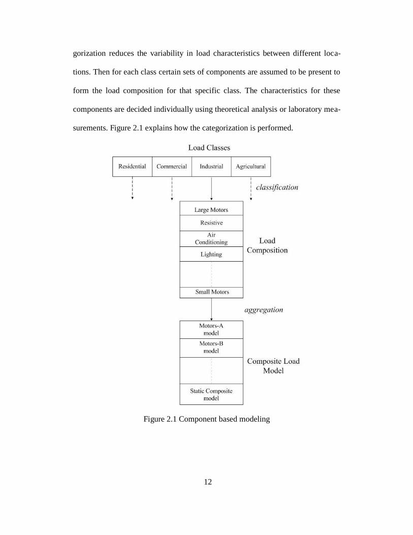
gorization reduces the variability in load characteristics between different loca-

tions. Then for each class certain sets of components are assumed to be present to

form the load composition for that specific class. The characteristics for these

components are decided individually using theoretical analysis or laboratory mea-

surements. Figure 2.1 explains how the categorization is performed.

Figure 2.1 Component based modeling

13

This approach has the advantage of being more realistic than the mea-

surement method because it has the flexibility of including all types of loads ex-

plicitly, including dynamic behavior of rotating loads.

However, this approach has a major drawback which is the need for data

describing the present class mixes and components included in each mix. This can

be achieved by thorough surveys from various utilities.

2.4 Static Composite Load Model (ZIP)

From the previous discussion it is obvious that more than one single static

load model is needed to describe the behavior of load aggregation. This is due to

the fact that different load components with different characteristics were embo-

died into a single entity [6, 7, 13]. Static composite load model was developed to

represent the complex relation between power and voltage magnitude through an

algebraic relation that combines the three different static load models (constant

impedance Z, constant current I, constant power P), hence it is sometimes called

ZIP model.

A polynomial equation is usually used to represent the composite static

model as follows:

(2.1)

(2.2)

where is the rated (or initial) voltage, and are the active and reactive

power, respectively, consumed at , and are coefficients that specify

the portions of load of which their real power corresponds to constant impedance,

14

constant current and constant power respectively. The summation of these coeffi-

cients equals 1. The terms , and are the reactive power corresponding

coefficients. It can be noticed that a frequency dependency linear term has been

added to both equations to capture frequency change effect over power consump-

tion response. is the deviation in frequency from nominal value, and

are the frequency sensitivity of active and reactive power respectively.

The polynomial model has limited flexibility in representing highly vol-

tage sensitive and nonlinear loads. For example the reactive power of discharge

lighting is proportional to voltage to the power four [15]. Therefore, an exponen-

tial model which provides more flexibility can be used. The exponential compo-

site static model is as follows:

(2.3)

(2.4)

It can be noted that the exponential form is more general than the polynomial one,

since by assigning the exponentials and the values 2 and 1 respectively

the polynomial model can be realized.

2.5 Motor Modeling

Rotating loads which include all the different types of motors are respon-

sible of the dynamic behavior loads have during transients. Previous discussed

static models are not able to capture these dynamics due to the high nonlinearity

and discontinuity in motors behavior under depressed voltage levels. Motors can

occupy around 72% of the total load [16], especially in areas with summer load

15

peak where air conditioners (A/C) are intensively used. Most of the industrial load

is also comprised of motors. In the case of certain industrial loads motors can

represent around 98% of the total load [17].

With this high motor load penetration, dynamic behavior becomes very

significant and important to capture in transient studies, especially in short term

voltage stability analysis. Voltage recovery delay -or even collapse- following a

fault is directly related to decelerating and stalling motors as will be explained

next. Two types of motors will be discussed:

Three phase induction motors

Single phase A/C motors

Those two types were chosen because they are the most commonly used motors,

and have the largest impact over voltage stability [7, 10].

Three phase induction motors

The key factors in determining a motor active and reactive power response

to voltage variations are the inertia (motor and load shaft inertia) and rotor flux

time constant [6]. Therefore, it is desirable to differentiate between large and

small induction motors according to their inertia, since motors with low inertia

tend to decelerate and stall faster than large motors.

In steady state operation, the motor electrical torque is equal to the me-

chanical torque of the mechanical load connected to it. However, under voltage

disturbance (usually depressed voltage magnitude due to a fault) the generated

electrical torque is reduced depending on the voltage magnitude, since the elec-

trical torque is proportional to the voltage squared. This state of non-equilibrium

16

between electrical and mechanical torque will cause the motor to decelerate. The

deceleration rate depends on the applied voltage level and on the mechanical load

characteristics. Mechanical load torque can be either speed dependant (fans,

pumps, etc.) or constant (reciprocating and rotary compressors), naturally constant

torque will cause higher deceleration rate. During deceleration the slip will pro-

portionally increase causing the motor to draw high current at low power factor.

The increased consumption of reactive power is responsible for delaying the vol-

tage recovery and can even cause a voltage collapse. If the fault is not cleared

promptly, and there is not enough reactive power, motors will decelerate till they

stall. Figure 2.2 shows typical torque and current characteristics for an induction

motor.

Figure 2.2 Induction motor torque and current curves

17

2.5.1 Induction Motor Modeling

To capture the previously mentioned phenomena associated with induction

motors, a dynamic model is required. Three models that describe induction motor

exist [13]:

First order induction motor model: a purely dynamic mechanical

model that neglects internal electric dynamics.

Third order induction motor model (single cage rotor model): in-

cludes rotor flux dynamics along with mechanical dynamics.

Fifth order induction motor model (double cage rotor model): in-

cludes mechanical dynamics, rotor flux dynamics and stator flux

dynamics.

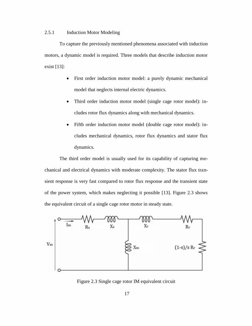
The third order model is usually used for its capability of capturing me-

chanical and electrical dynamics with moderate complexity. The stator flux tran-

sient response is very fast compared to rotor flux response and the transient state

of the power system, which makes neglecting it possible [13]. Figure 2.3 shows

the equivalent circuit of a single cage rotor motor in steady state.

Figure 2.3 Single cage rotor IM equivalent circuit

18

2.5.2 Single Phase A/C Motor

The dominant power consuming part of the single phase air conditioner

units is the compressor motor, it consumes up to 87% of the total unit consump-

tion [9]. Therefore, this type of motors have to be modeled and considered in tran-

sient studies, especially in areas which have summer load peaks. Single phase

A/C motors are prone to stall because of their low inertia and the mechanical cha-

racteristics of the compressor they drive [11, 14], therefore, they are directly re-

sponsible for the delayed voltage recovery phenomenon. Under stall conditions

(i.e. slip=100%) motors draw very high current with a very low power factor, the

amount of this current is only determined by motors rated locked-rotor current

and the applied voltage. In some cases this current can be as high as 8.5 p.u. for

residential A/C [14]. Similar to induction motors, under reduced voltage condi-

tions the electrical torque will start to drop down causing the motor to decelerate.

The motor will continue to decelerate until it is unable to overcome the pressure

applied by the compressor, at this point the motor stalls. Usually single phase A/C

motors stall if the voltage falls to between 50 – 65 % of nominal voltage for more

than 3 cycles [15]. Stalling voltage depends on other factors, such as: ambient

temperature and humidity. Figure 2.4 shows the reactive power consumption of a

stalled A/C motor.

19

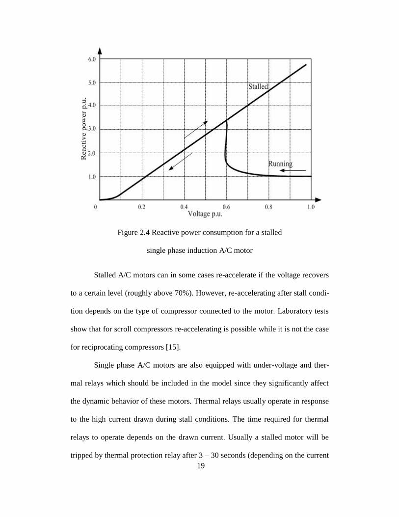
Figure 2.4 Reactive power consumption for a stalled

single phase induction A/C motor

Stalled A/C motors can in some cases re-accelerate if the voltage recovers

to a certain level (roughly above 70%). However, re-accelerating after stall condi-

tion depends on the type of compressor connected to the motor. Laboratory tests

show that for scroll compressors re-accelerating is possible while it is not the case

for reciprocating compressors [15].

Single phase A/C motors are also equipped with under-voltage and ther-

mal relays which should be included in the model since they significantly affect

the dynamic behavior of these motors. Thermal relays usually operate in response

to the high current drawn during stall conditions. The time required for thermal

relays to operate depends on the drawn current. Usually a stalled motor will be

tripped by thermal protection relay after 3 – 30 seconds (depending on the current

20

magnitude). Thermal tripping could happen for an individual unit or for a whole

feeder that is supplying many stalled motors. Under-voltage protection contactors

operate faster than thermal ones, actually under-voltage contactors open almost

instantaneously at low voltages (35 – 45 %), and can reclose at voltages above

50% [9].

2.5.3 Single phase A/C motor modeling

The characteristics of single phase A/C motors discussed above have sig-

nificant impact on short term voltage stability analysis and must be included in

the model. The controls and protection schemes should also be included in the

load model since they control tripping and reconnecting the units. Laboratory tests

and offline simulations have proved that three phase induction motor model is not

adequate to capture the dynamic response of single phase A/C motors [1], espe-

cially the stalling conditions. However, the steady state behavior of both motors is

very similar and a three phase induction motor can be suitable to capture the be-

havior of single phase A/C motor in steady state conditions. To include the stal-

ling conditions, a fictitious shunt component is connected in parallel with the mo-

tor to replace it with the locked-rotor impedance representing a constant imped-

ance model. This approach is called “hybrid performance based modeling” [15].

2.6 Composite load model structure

The Western Electricity Coordinating Council (WECC) developed an inte-

rim composite load model that was used for planning and operation studies in ear-

ly 2002 [9]. This model was represented by 80% of load as static, and 20% as in-

duction motor load. This interim model was unable to represent delayed voltage

21

recovery events following a major transmission fault. Simulations using this inte-

rim model indicated instantaneous voltage recovery contrary to the real recorded

event. Therefore, WECC formed a load modeling task force (LMTF) to improve

the interim model and develop a more accurate and comprehensive one. The

LMTF acknowledged the following factors in the improved composite load mod-

el:

The electrical distance between the point where the load is connected in

simulations (usually transmission or sub-transmission level) and the point

where the physical load is connected (distribution level). Therefore, the

improved model will include the network components such as: feeders

and transformers impedance, shunt devices, protection, transformer taps,

etc.

Single phase A/C motors have very significant impact over voltage sta-

bility and should be included in the new model explicitly since the induc-

tion motor model is not adequate to represent their characteristics. This

will allow the new composite model to capture the dynamic behavior of

these motors such as: decelerating, stalling, tripping, etc.

Induction motors vary widely in characteristics depending on size, num-

ber of phases and mechanical torque they drive. Therefore, the new mod-

el should differentiate between the different types of induction motors.

This provides more flexibility and accuracy in representing motor loads.

Figure 2.5 shows LMTF proposed composite load model.

22

Figure 2.5 LMTF proposed composite load model

23

CHAPTER 3

VOLTAGE STABILITY AND VAR COMPENSATION

3.1 Introduction

Voltage stability is the ability of a power system to maintain steady ac-

ceptable voltages at all buses in the system under normal operating conditions and

after being subjected to a disturbance [18]. Disturbances could be large such as

major transmission faults, generating unit tripping, loss of major components or

small such as a gradual change in load. Voltage instability occurs when one sys-

tem bus -or more- suffers from progressive and uncontrolled change in the voltage

magnitude, usually in the form of voltage decrease. Voltage instability can cause

prolonged periods of voltage depression conditions (brownout), or even a voltage

collapse and blackout depending on the available reactive power and load dynam-

ics. Although voltage instability is essentially a local phenomenon, however vol-

tage collapse which is more complex than simple voltage instability and is usually

the result of a sequence of events, is a condition that affects large areas of the sys-

tem [18].

Rotor (angle) stability had been the primary aspect of stability studies for

decades. However, recent events of abnormal voltage magnitudes and voltage col-

lapse incidents in some large interconnected power systems have sparked the in-

terest in the voltage stability phenomenon [2, 19]. Rotor stability was believed to

be responsible of voltage instability conditions. This case is true since a gradual

loss of synchronism of machines as rotor angles between two groups of machines

approach or exceed 180° would result in very low voltages at intermediate points

24

in the network. However, this is not the case if the disturbance was close to load

centers and the voltage depression was rather caused by load dynamics and reac-

tive power deficiency. Therefore, voltage instability may occur when rotor stabili-

ty is not an issue. Actually, sustained voltage instability conditions can cause rotor

instability [18].

Several recent factors and operating conditions have also caused the vol-

tage instability problem to become more prevalent, such as [20, 21]:

Power systems in general and specifically transmission lines tend to be

operated under more stressed conditions. This stressed operating condition

is not only due to continuous and significant load growth, but also because

of major changes and restructuring of energy markets. Stressed transmis-

sion lines have less capability of delivering reactive power to demanding

load centers because of the high reactive power losses. Transmission lines

(especially long ones) with relatively large voltage angle difference be-

tween sending and receiving ends also have limited capability of reactive

power delivery.

High rates of induction and single phase motor penetration, especially

those used in air conditioning systems, heat pumps and refrigeration.

These motors are known as low inertias machines, as a result they have

fast response to disturbances. Voltage instability issues are directly related

to dynamic behavior of motors.

Electronic loads which have significant discontinuous response to varia-

tions in voltage magnitude.

25

The use of HVDC tie lines to transfer large amounts of electric power. The

convertors associated with these lines consume significant amounts of

reactive power.

Excessive reliance on shunt connected capacitor banks for reactive power

compensation. In heavily shunt capacitor compensated systems, the vol-

tage regulation tends to be poor. Another disadvantage for shunt capaci-

tors is that the reactive power support they provide is directly proportional

to the square of the voltage. Therefore, at low voltage when the reactive

power support is most needed, the VAr output of the capacitor banks

drops.

3.2 Classification of Voltage Stability

It is useful to classify voltage stability into subclasses in order to better

understand the system behavior under voltage instability conditions. Classifica-

tion also helps choosing the right analytical strategies depending on the nature of

the phenomenon of interest. Voltage stability is classified here according to the

magnitude of the disturbance affecting the system into two subclasses [18]:

Small disturbance voltage stability: also called small-signal or steady-

state voltage stability. This type of voltage stability is related to small

and possibly gradual perturbations in the system, such as small changes

in the load. Small-signal stability is determined by the characteristics of

load and continuous and discrete controls at a specific instant of time.

A criterion for this type of voltage stability is that at a given operating

condition, for every bus in the system, the bus voltage magnitude in-

26

creases as the injected reactive power at the same bus is increased.

When analyzing small disturbance voltage stability usually either mid-

term (10 seconds to few minutes) or long-term (few minutes to tens of

minutes) studies are performed.

Large disturbance voltage stability: also called transient voltage stabili-

ty. Large disturbance here refers to major changes in operating condi-

tions. These changes could be major faults on transmission lines, gene-

rating units tripping, transmission lines tripping, or other large distur-

bances. The transient voltage stability is determined by the load charac-

teristics, continuous and discrete controls, as well as the protection sys-

tems. However, in order to capture the nonlinear dynamic interactions

between the different system components and their effect on transient

voltage stability, a dynamic time domain analysis should be performed.

This type of analysis is referred to as short-term voltage stability analy-

sis (0 to 10 seconds). A criterion for large disturbance voltage stability

is that following a large disturbance and after the actions of system

control devices, voltages at all buses reach acceptable steady state le-

vels.

3.3 Voltage Stability Analysis

From the previous discussion it is apparent that each subdivision of vol-

tage stability has its own characteristics and nature, therefore each type has to be

approached and analyzed using the appropriate analytical tool. In general, voltage

stability problems are studied by two approaches [18, 22]:

27

Static analysis

Nonlinear dynamic analysis

3.3.1 Static Analysis

Static analysis studies are used for steady state voltage stability problems

initiated by small disturbances. The system dynamics affecting voltage stability in

the event of small disturbances are usually quite slow and much of the problem

can be effectively analyzed using the static approaches that examine the viability

of a specific operating point of the power system [18]. Power flow is used for this

type of study, where snapshots are captured from different system conditions at

certain time instants. At each of these time frames system dynamic equations are

linearized, and time derivatives of the state variables are assumed to be zero,

while state variables take their numerical value at that time instant. Therefore, the

resultant system equations are simple algebraic equations that can be solved using

power flow simulation.

Static analysis can be performed faster than dynamic simulations and

needs less modeling details. However, with the presence of fast acting compo-

nents such as motors, and HVDC convertors, the dynamic effect and the interac-

tions between controllers and protection must be included in the voltage stability

analysis to capture the actual behavior of the system [18, 23].

Steady state static studies are not only useful in the determination of the

voltage stability of a given operating conditions, but they also provide information

about the proximity of these conditions to voltage instability, as well as voltage

sensitivity. Static analysis has been solved by different approaches [18, 23]:

28

V-Q sensitivity analysis: The linearized region provided by power flow

analysis around a given point is used to indicate the relation sensitivity between

the voltage and reactive power. This sensitivity is described by the elements of the

Jacobian matrix. The power equation equations (polar form) for any node i can be

written as

(3.1)

where, is the complex, real and reactive power injections at bus i respec-

tively. The term is the bus voltage, and is the conjugate current injected at

bus i.

Power flow equations (real form) of bus i with respect to the rest of the

system are written as

(3.2)

(3.3)

where, G and B are the real and imaginary parts of the admittance matrix respec-

tively. is the voltage angle difference between buses i and m. The Jacobian

matrix is used to achieve the following linearized form

(3.4)

where, are the incremental changes is bus real power, reactive

power injection, voltage angle and voltage magnitude respectively. Although sys-

tem stability is affected by the real power, it is possible to keep P constant in or-

29

der to evaluate the sensitivity only between the reactive power and voltage magni-

tude. Therefore by setting

(3.5)

where is the reduced Jacobian matrix of the system and can be written as,

(3.6)

The V-Q sensitivity at a bus represents the slope Q-V curve at a given op-

erating point. A positive value for the sensitivity indicates stable conditions. The

larger the sensitivity index the closer is the operating point to instability. The val-

ue of infinity represents stability limit or the critical point. Negative values for

sensitivity indicate unstable conditions, with very small negative values

representing highly unstable conditions.

Q-V modal analysis: This analysis approach has the advantage of provid-

ing the mechanism of instability at the critical point. The eigenvalues and eigen-

vectors of the reduced Jacobian matrix are evaluated and used to indicate voltage

stability. Positive eigenvalues represent stable voltage conditions, and the smaller

the magnitude, the closer the relevant modal voltage is to being unstable.

Compared to V-Q sensitivity analysis, Q-V modal analysis is more capable

of identifying the voltage stability critical areas and elements which participate in

each mode once the system reaches the voltage stability critical point, hence, it

can describe the mechanism of voltage instability. V-Q sensitivity analysis is not

able to identify individual voltage collapse modes; instead they only provide in-

formation regarding the combined effects of all modes of voltage-reactive power

variations.

30

V-Q curve analysis: V-Q curves show the relationship between the reactive

power support at a certain bus and the voltage of that same bus. For large power

systems these curves are obtained by a series of power flow simulations. A ficti-

tious synchronous condenser with unlimited reactive power capability is placed at

the test bus, and the voltage magnitude is varied through the simulation [24].

V-Q curves are useful in determining the amount of reactive power needed

to be injected at a certain bus in order to obtain a desired voltage level. Therefore,

these curves can be used for both; voltage stability indication purposes, and shunt

compensation sizing. However, it should be noted that V-Q curves are only valid

for steady state analysis [2]. It should also be noted that power flow equations

tend to converge around the voltage stability critical point, therefore, special tech-

niques have to be used to overcome the divergence problem, such as continuation

power flow.

3.3.2 Nonlinear Dynamic Analysis

Dynamic analysis provides the most accurate results for voltage stability

phenomenon using time domain simulations which capture the real dynamic na-

ture of the system without any approximations. Nonlinear dynamic simulation is

therefore very useful and effective for short term voltage stability studies and fast

voltage collapse situations following large disturbances [22]. However, as a price

for this accuracy, dynamic simulations are much more complicated than static

studies since the overall system equations include first-order differential equations

that have to be solved as well as the regular algebraic equations. Solving these

equations requires significant computational capacity and is relatively time con-

31

suming. Dynamic simulation results accuracy depends mainly on the models used,

therefore, system components have to be modeled in details and with high accura-

cy [18].

The system set of differential equations can be expressed as follows:

(3.7)

And the set of algebraic equations as:

(3.8)

where, are the initial conditions, x: state vector of the system, V: bus vol-

tage vector, current injection vector, YN: bus admittance matrix.

Although no expression for time appears explicitly in the previous equa-

tions, however, YN is a function of both voltage and time since certain time vary-

ing components such as transformer tap changer, phase shift angle controls, etc.

are included in it. Also, the relation between I and x can be a function of time

[18]. Numerical integration alongside with power flow analysis is usually used to

solve the nonlinear dynamic equations in the time domain.

3.4 Reactive Power Support Measures

The previous discussion illustrates the direct effect reactive power has

over voltage magnitudes and consequently over the overall system voltage stabili-

ty. A fundamental aspect of controlling the voltage levels throughout the system

is reactive power balance, and hence compensation is considered. Depending on

the operating conditions, system components could be either absorbing reactive

power, such as: loads in general and heavily loaded transmission lines, or supply-

ing reactive power, such as: underground cables or transmission lines with very

32

light load. However, since the usual issue with voltage stability is under-voltages

(as a result of disturbances) and heavily stressed transmission lines, reactive pow-

er injection is usually needed. It should also be noted here that reactive power

compensation increases the active power transfer capabilities, and reduce the sys-

tem losses (increase efficiency). Several techniques are used as reactive power

compensation measures, such as [18, 24]:

Synchronous condensers

Series capacitors

Shunt capacitor banks

Shunt reactors

Static VAr systems.

3.4.1 Synchronous Condensers

A synchronous condenser is a synchronous machine running without a

prime mover or mechanical load, usually in over-excitation mode [18]. The

amount of reactive power supplied (or absorbed) by this machine is controlled by

controlling the field excitation current. Synchronous condensers need to be sup-

plied with small amounts of active power to supply losses, and they are consi-

dered as active shunt compensators. Synchronous condensers have the following

advantages:

Instantaneous response to voltage variations.

The ability of producing constant reactive power regardless of the

system voltage level.

33

Their maximum output reactive power limits can be exceeded for cer-

tain period of time.

However, synchronous condensers main disadvantage is their high initial

and operating costs.

3.4.2 Series Capacitors

Series capacitors can be connected either to distribution feeders or high

voltage transmission lines [18]. However, series capacitors are more commonly

used in high voltage transmission lines because of the long distance of these lines.

Series capacitors are used to reduce the net transmission line inductive reactance

and therefore they reduce the reactive power losses through the line, and increase

active power transfer capabilities, as well as improving transient stability [24].

Since they are connected in series with the line reactance, the reactive output

power of series capacitors is self regulated and is proportional to the square of the

current. Therefore, series capacitors output reactive power will increase at high

load currents when it is most needed almost instantaneously.

However, series capacitors have the following disadvantages and compli-

cations:

Subsynchronous resonance phenomenon.

Overload for parallel line outages. An outage of one line in a 2 circuit

transmission line with almost double the current in the remaining cir-

cuit, this will cause the series capacitor to quadruple.

Overvoltage profiles at one side of the transmission line under high

load currents.

34

3.4.3 Shunt Capacitor Banks

Whether the shunt capacitor banks are installed in the transmission or the

distribution network, the main purpose of using them is to improve the lagging

power factor and bring it close to unity. Therefore, shunt capacitors provide local

reactive power for load centers instead of importing this power from remote sites

which increases the system efficiency. Shunt capacitor banks are also useful in

allowing nearby generating units to operate near unity power factor, and there-

fore, maximizing fast acting reactive reserves [24]. Since shunt capacitor banks

provide reactive power, they are also used as effective voltage regulators. Shunt

capacitor banks are usually located on load buses but can also be installed on dis-

tribution feeders for feeder voltage control purposes.

Shunt capacitor banks are usually connected to the system through me-

chanical switches. These switches can be controlled manually, by under-voltage

relays, or by timers. Shunt capacitor banks have the following advantages [18,

24]:

Low implementation and maintenance cost

Flexibility in installation and operation

Require simple control schemes.

However, shunt capacitor banks have the following limitations and disad-

vantages [18, 24]:

Output reactive power produced is directly proportional to the voltage

squared. Consequently, the reactive power output is reduced at low vol-

35

tages when it is likely to be needed most (i.e. following a large distur-

bance).

Mechanical switching is slow compared to power system transients. As a

result, shunt capacitor banks are not capable of improving short term vol-

tage stability (i.e. they cannot prevent motor stalling for example).

Following a large disturbance, if the affected part of the system was iso-

lated, the stable part may encounter very high over-voltages because of

energizing the shunt capacitor banks during the period of voltage decay.

3.4.4 Shunt Reactors

In contrast to shunt capacitor banks, shunt reactors are used to regulate

voltage by consuming the excess reactive power in a transmission line, and there-

fore, preventing over-voltages. Switched shunt reactors can also be disconnected

from the system to reserve the available reactive power in the case of depressed

voltages.

3.4.5 Static VAr Systems

Static VAr compensators (SVCs) are also shunt connected and used to im-

prove voltage stability by either producing or absorbing reactive power. The term

static indicates that SVCs do not contain any moving parts, such as rotating com-

ponents in synchronous condensers, and mechanical switches in shunt capacitor

banks. Instead, solid state switches are used to vary the SVCs net susceptance and

consequently the overall output. This feature makes SVCs suitable for transient

voltage support because they can respond to voltage variations within few cycles

[2, 18]. Static VAr system (SVS) includes SVCs and mechanically switched ca-

36

pacitors or reactors whose outputs are coordinated in a single shunt connected

unit.

The following are the mostly commonly used techniques in achieving a vari-

able susceptance [2]:

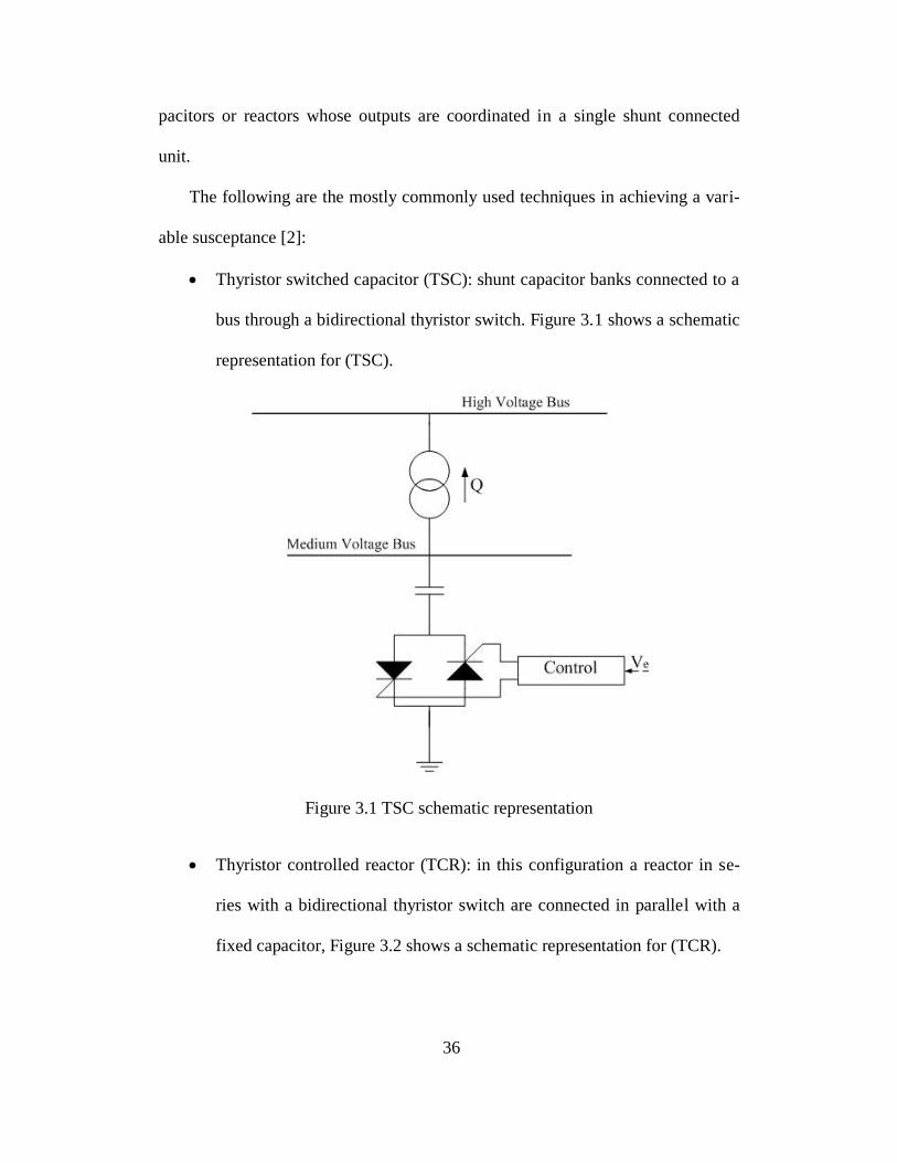
Thyristor switched capacitor (TSC): shunt capacitor banks connected to a

bus through a bidirectional thyristor switch. Figure 3.1 shows a schematic

representation for (TSC).

Figure 3.1 TSC schematic representation

Thyristor controlled reactor (TCR): in this configuration a reactor in se-

ries with a bidirectional thyristor switch are connected in parallel with a

fixed capacitor, Figure 3.2 shows a schematic representation for (TCR).

37

Figure 3.2 TCR schematic representation

In both types the output susceptance is controlled by the firing angle of the

thyristors. A controller is used to provide the thyristors with the firing signal de-

pending on the desired output. In steady state operation, the reactive power output

of the SVC is:

(3.9)

where, V is the bus voltage, and B is the net output susceptance. B can be

represented as:

(3.10)

subject to:

38

where, K is the SVC gain, V0 is the reference voltage, V is the actual bus voltage,

Bmin, Bmax are the minimum and maximum allowed susceptance values, respec-

tively.

At the boost limit, the SVC becomes a fixed shunt capacitor. Therefore, it

is desirable to supplement the SVC with mechanically switched capacitors in or-

der to maintain the controllability characteristics of the SVC. Mechanically

switched capacitors also help to reset the SVC to its initial set point following a

disturbance in order to preserve its output for future operation.

Despite the relatively high initial costs, SVCs have been widely used in

power systems because of their fast and precise voltage regulation capabilities

which help improving the system transient voltage stability following a large dis-

turbance. As mentioned before, a major disadvantage of SVCs is that at their

maximum output they behave as regular shunt capacitors and the reactive power

produced is directly proportional to the square of the voltage.

To overcome this problem, a static compensator (STATCOM) is used.

Similar to synchronous condenser, STATCOM has an internal voltage source

which provides constant output current even at very low voltages. Therefore, the

output reactive power of the STATCOM is linearly proportional to the bus vol-

tage. Figure 3.3 shows both, SVC and STATCOM characteristics curves [21].

39

Figure 3.3 SVC and STATCOM characteristic curves

40

CHAPTER 4

PROPOSED METHODOLOGY

4.1 Motivation

Sufficient reactive power is needed in a power system to achieve normal

ac voltage levels to ensure voltage stability. However, if the system is affected by

a large disturbance, reactive power consumption will be increased throughout the

system and could cause significant depression in voltage magnitudes, especially at

load buses. Therefore, reactive power compensation becomes essential to avoid

short term voltage instability, or even a fast voltage collapse. The amount of reac-

tive power needed and the instant when this power should be provided become

very important in systems heavily loaded with motors and/or any other fast acting

dynamic devices. Small motors decelerate very fast with reduced voltages and

tend to stall if the ac system voltage does not recover to higher levels promptly.

Therefore, the location and amount of VAr compensation should be determined

optimally in order to support the short term voltage stability with the least possi-

ble cost.

4.2 Objective

The objective of this work is to develop a comprehensive methodology

which can determine the optimized VAr compensation (location and level) that is

needed to maintain the system short term voltage stability, following a large dis-

turbance close to load centers. This approach should be valid for a range of oper-

ating conditions and contingencies. In contrast to previous approaches, this work

evaluates the reactive power needs dynamically and in the transient time frame.

41

4.3 Static Analysis

In order to illustrate the method of reactive power optimization, this work

uses a 162-bus, 17-generator, IEEE test case as the base case. A contingency scan

was performed by applying a three phase fault at different 345 kV buses. Since

short term voltage stability and delayed voltage recovery are directly related to

load behavior, the faults were applied at buses close to load centers, and the vol-

tage levels of load buses were monitored. Each fault was cleared after 6 cycles by

opening a 345 kV line. The fault that caused the deepest voltage dips at load buses

was chosen as the most severe contingency and used in the dynamic simulation.

The loads that were most affected by that contingency were chosen to be assigned

dynamic load models. These load centers were also stepped down through distri-

bution transformers from the 69 kV voltage level to 12.47 kV. Representing loads

in the distribution level provides the opportunity to include network effects and

achieve more accurate results.

4.4 Dynamic Models

As was explained in the load modeling chapter, dynamic load models, and

dynamic models in general are essential to capture the dynamic behavior of the

system, especially with high motor loads and during transients. The following dy-

namic models are used for simulating the base case in time domain:

Load composite model (cmpldw): this model was assigned to the

load buses close to the most severe contingency (12 buses). It also

contains the parameters for the different types of motors it

represents.

42

Synchronous generator (gencls): it represents the classical genera-

tor model (8 generators).

Solid rotor generator (genrou): represented by equal mutual in-

ductance rotor modeling (9 generators).

Excitation system (exac1): IEEE type AC1 excitation system (9

generators).

Over-excitation limiter (oel1): over-excitation limiter for syn-

chronous machines excitation systems (9 generators). These mod-

els were added after it was noticed that some generators exceeded

their reactive power capabilities following a large disturbance.

Static VAr device (svcwsc): SVC model, compatible with WSCC

standards (12 SVCs).

Bus voltage recorder (vmeta).

4.5 Trajectory Sensitivity Index

Trajectory sensitivity index method has been used to investigate the vol-

tage stability of the power system. Trajectory sensitivity index has also been

found to be useful in finding the proper location for fast dynamic reactive power

support [16]. In this work, trajectory sensitivities are used as weights in the objec-

tive function of the optimization problem since they describe the voltage response

of load buses when reactive power is injected at a transmission or sub-

transmission level bus. The trajectory sensitivity index (TSI) can be evaluated us-

ing the following formula:

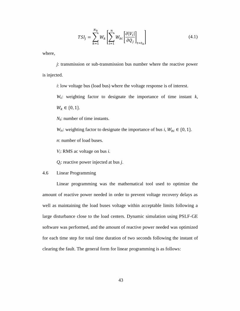
43

(4.1)

where,

j: transmission or sub-transmission bus number where the reactive power

is injected.

i: low voltage bus (load bus) where the voltage response is of interest.

Wk: weighting factor to designate the importance of time instant k,

.

Nk: number of time instants.

Wbi: weighting factor to designate the importance of bus i, .

n: number of load buses.

Vi: RMS ac voltage on bus i.

Qj: reactive power injected at bus j.

4.6 Linear Programming

Linear programming was the mathematical tool used to optimize the

amount of reactive power needed in order to prevent voltage recovery delays as

well as maintaining the load buses voltage within acceptable limits following a

large disturbance close to the load centers. Dynamic simulation using PSLF-GE

software was performed, and the amount of reactive power needed was optimized

for each time step for total time duration of two seconds following the instant of

clearing the fault. The general form for linear programming is as follows:

44

(4.2)

where,

f: is the objective (cost) function, presented as a vector.

x: the set of variables, presented as a vector.

lb and ub: are the lower and upper bounds allowed for the variables, pre-

sented as vectors.

A and Aeq: are the constraints inequality and equality matrices respectively.

The objective function to be minimized is the total injected reactive power with

constraints on the voltage level and SVC size. The optimization approach is for-

mulated as follows:

Let Sj(t) represents the trajectory sensitivity of bus j at the time instant t;

(4.3)

The trajectory sensitivities are used as weights in the objective function as fol-

lows:

(4.4)

And the constraints are,

(4.5)

(4.6)

where,

45

are the acceptable predefined minimum and maximum RMS

voltage levels at load bus i, respectively, at all time instants.

: is the uncompensated RMS voltage level at load bus i at instant t

(without VAr injection)

: are the allowed minimum and maximum amounts of VAr in-

jection, respectively.

The trajectory sensitivity Sj(t) is calculated by injecting 1 p.u. of reactive power at

bus j, and for each j summing up the voltage level changes at load buses for all i,

for each time step.

It should be noted here that the voltage level constraint in equation (4.5) is

considered as a conservative constraint since it assumes that simultaneous VAr

injections at different buses will result in voltage increments that are all in phase

with each other. However, study results presented in Chapter 5 show that the vol-

tage levels increased in each time step when optimal VArs are injected at optimal

locations. This proves that the approximation introduced by this inequality is mi-

nimal, and that the phase shift between voltage increments is not significant since

voltages add up for each time step, resulting in a higher overall voltage magni-

tude.

For time steps following the fault clearance instant, voltage magnitude

will still be very low (depending on the disturbance severity) even with VAr in-

jection since voltage at load buses cannot be recovered to its normal values in-

stantaneously. Therefore, it is more realistic to have a changing value for

that would be increased gradually in each time step. In this work was cho-

46

sen to be directly related to for each time step, which makes

time de-

pendant as well. In this work the minimum allowed voltage level for each time

step is defined as follows:

(4.7)

Therefore, at each time step the optimization function will calculate the least

required amount of VAr injection needed to increase the voltage level by 15%

above its uncompensated value for each load bus. The value of 15% increase was

chosen for the following reasons:

It provides a realistic recovery rate for voltage levels at load buses.

It provides acceptable voltage levels for the last time step in the optimiza-

tion process; after two seconds of clearing the fault, the lowest voltage

level is around 0.7 p.u.

It minimizes the number of unsolved (infeasible) cases in the optimization

process.

It should be noted here that is assigned a maximum value (i.e. 0.95

p.u.) to ensure that it is always kept below .

is considered to be 1.05

p.u. although it does not affect the optimization results since it is a minimization

problem.

4.7 Generalizing Results

Since the optimization process is performed for each time step, the out-

come of this procedure is a set of optimized values of Qj for each time step as

well. Each set contains the values of VAr injection needed by each SVC. In order

to achieve one set of VAr injection optimal values that represents all the sets at

47

different time steps, an averaging procedure is required. However, in the averag-

ing process higher weights should be assigned to the more critical time steps. Crit-

ical time steps here refer to the time steps following the fault clearing instant

when the voltage levels are at their lowest point. VAr compensation is needed the

most at these critical time steps to prevent voltage recovery delays caused by mo-

tors stalling. The optimized objective function value will be relatively low at these

critical time steps because is at its lowest levels. Therefore, a weighting

factor that is inversely proportional to the objective function value is used for

each time step. This will ensure that the VAr compensation needs for these critical

time steps will have better representation in the overall average for all time steps.

The weighted sets are then averaged over all the time steps to evaluate the final

optimal VAr injection values. The averaging procedure can be presented as fol-

lows:

(4.8)

where,

QT: is the total weighted and averaged set of VAr injection values.

f(Qj): is the value of the objective function at a given time instant.

This new total set of VAr injection values represents a single operating condition

and contingency case, while the objective of this work is to find a set of VAr

compensation values that is valid for different operating conditions and contin-

gencies. Therefore, the load at the buses that are being investigated (i buses) was

increased in order to change the operating conditions by representing load growth.

48

The load was increased by 5%, 15% and 20%. For each new operating condition,

the voltage sensitivities were recalculated, and the optimization and averaging

procedures were performed again. Consequently, four sets of the total weighted

and averaged VAr injection values were generated; one for the base case (no load

increase), and three for the increased load cases. In order to compose a final set of

VAr compensation values that represents the different operating conditions, the

highest value of VAr compensation was chosen from each case set for every bus.

Therefore, in the final optimized set of VAr compensation values, each SVC was

assigned its highest value in the different operating conditions. For different con-

tingencies, there is no need to run the whole process again since the base contin-

gency chosen is considered to be the most severe. Therefore, different contingen-

cies were used to validate the final set of VAr compensation values (SVC sizes).

49

CHAPTER 5

STUDY RESULTS

5.1 System Representation

An IEEE, 162-bus, 17-generator test case [26] is used throughout this

work. This test case consists of one area and twelve zones. Table 5.1 shows the

overall system components. The total generation is 15,546 MW, while the total

load is 15,387 MW.

Table 5.1 System components

Component Number

Buses 162

Generators 17

Shunts 34

Lines 238

Transformers 46

Load Aggregations 89

5.2 Base Contingency Selection

In order to select the most severe credible contingency, several three-

phase faults were applied at several 345 kV buses located near major load centers,

and the voltage dips at the 69 kV load buses were monitored. These faults were

cleared after 6 cycles by opening a 345 kV line. The criteria for selecting the most

severe contingency are the magnitude of voltage dips at load buses, and the num-

ber of affected buses by that contingency. Therefore, a contingency is considered

50

severe if it causes a significant voltage dips on a large number of load buses.

Worst Condition Analysis (WCA) feature in PSLF-GE was used to scan voltage

dips all over the system buses following a contingency. WCA scans for buses

whose voltage level change exceeds a predefined value for a certain amount of

time. In order to find the most severe contingency, a change percent in voltage

level of 50% for 0.1 seconds was chosen as the threshold for WCA. Therefore,

any bus whose voltage level dips below 50% of its initial level for 0.1 seconds or

more is recorded. This threshold is chosen since a 50% (or more) dip in voltage

level for at least 0.1 seconds at a load bus will very likely cause most of the run-

ning motors to stall. After running WCA for several contingencies, it was found

that a three-phase fault on bus 120 “S3456 3” would cause 12 load buses to vi-

olate the limit predefined in WCA. Table 5.2 shows the representative numbers,

voltage level and load. Figures 5.1-5.2 show the load buses affected by the most

severe contingency. It should be noted that these loads are represented by static

models and are located at the transmission voltage level. Voltage magnitude plots

have been divided into two graphs (sets) throughout this chapter for clarity pur-

poses.

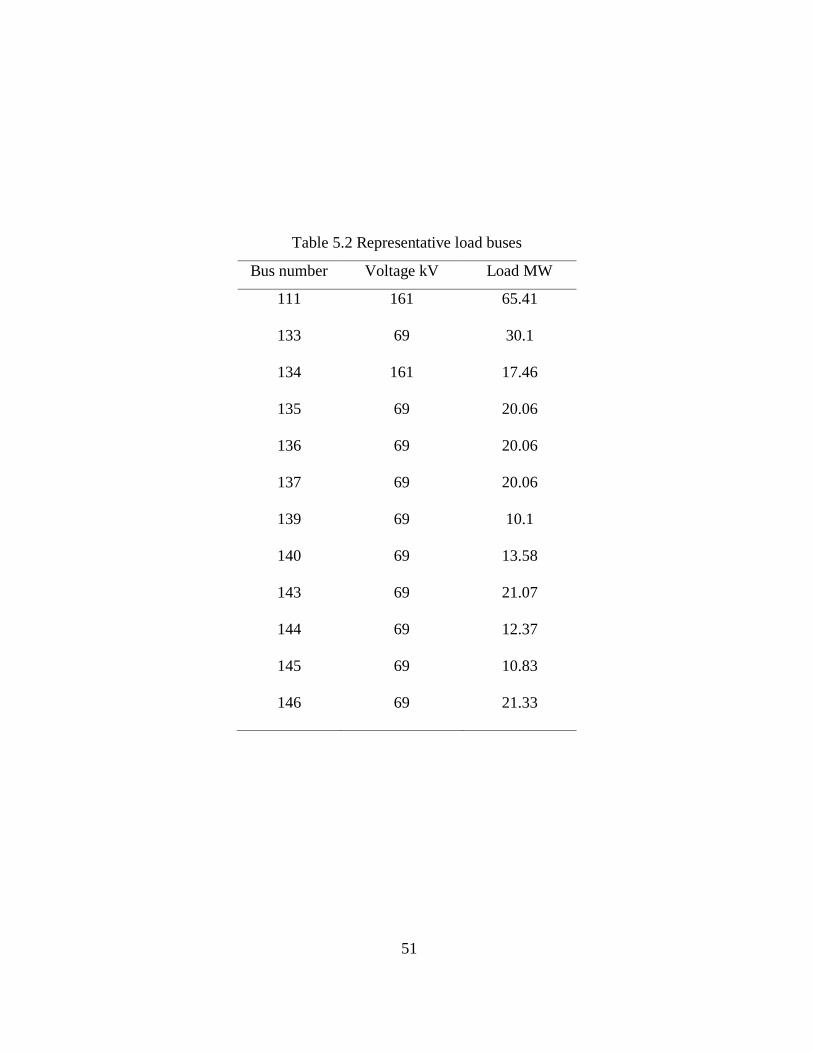
51

Table 5.2 Representative load buses

Bus number Voltage kV Load MW

111 161 65.41

133 69 30.1

134 161 17.46

135 69 20.06

136 69 20.06

137 69 20.06

139 69 10.1

140 69 13.58

143 69 21.07

144 69 12.37

145 69 10.83

146 69 21.33

52

Figure 5.1 Load bus voltage magnitude (static load models) set-1

Volt

age

mag

nit

ude

(pu)

Time (sec)

53

Figure 5.2 Load bus voltage magnitude (static load models) set-2

5.3 Dynamic Load Modeling

The power flow model for the test case used in this work represents the

system down to the sub-transmission level, and the loads are aggregated and con-

nected to the transmission or sub-transmission levels. Therefore, the load buses

represented in Figures 5.1-5.2 are either rated at 161 kV or 69 kV. In order to

represent the loads affected by the base contingency more realistically and accu-

rately, those 12 load buses were stepped down through distribution transformers

to the 12.47 kV level, and the new low voltage buses were assigned the numbers

163-174. It is also necessary to include motor models within the representative

load buses in order to capture the dynamic behavior of these loads. The impor-

Volt

age

mag

nit

ude

(pu)

Time (sec)

54

tance of dynamic models can be concluded from Figures 5.1-5.2; which show that

the voltage magnitude for those load buses recovered almost instantaneously de-

spite of the large disturbance which caused a significant voltage dip. The voltage

recovered to its normal value very fast because the dynamic behavior of motors,

such as: decelerating and stalling, is not represented in the static load models.

The composite load model provided by PSLF-GE (cmpldw) was used to

include motor models along with the static part of the load. The composite load

model (cmpldw) complies with the composite load model developed by WECC

LMTF shown in Figure 2.5. [27] cmpldw includes the models of the following:

Distribution network: This includes the substation components,

such as: transformers, shunts and feeders. However, this part was

not included in this work because the loads were already stepped

down to the distribution level.

Static loads: Part of the load was represented by static models.

The real power part of the static loads was represented as con-

stant current, while the reactive power part was represented as

constant impedance.

Motors: it is possible to represent up to four different motor types

in cmpldw. It is also possible to represent both, three-phase in-

duction motors as well as single-phase motors. In this work 72%

of the total load is assumed to be motors [1]. 10% of the motors

are modeled as large industrial motors (high inertia), while

55

around 50% of the motors are modeled as single-phase A/C mo-

tors, and the rest as small induction motors.

Figures 5.3-5.4 show the voltage magnitude for the representative load

buses after applying the base contingency. In these figures the loads were located

at the low voltage side of the network and represented by the composite dynamic

load model.

Figure 5.3 Load bus voltage magnitude (dynamic load models) set-1

Volt

age

mag

nit

ude

(pu)

Time (sec)

56

Figure 5.4 Load bus voltage magnitude (dynamic load models) set-2

Figures 5.3-5.4 show that when representing the dynamic models of mo-

tors the voltage recovery is delayed because of the deficiency in reactive power

caused by stalled motors. Figures 5.3-5.4 also show that some buses needed up to

4 seconds to partially recover after clearing the fault, while Figures 5.2-5.3 show a

full voltage recovery after less than 0.5 seconds after clearing the fault.

The voltage magnitudes in Figures 5.3-5.4 recovered to a value close to its

initial level because part of the stalled motors (60%) were allowed to reaccelerate

if their voltage magnitude increases to 0.7 p.u. Therefore, each time the stalled

motors at a certain load bus start to reaccelerate, the voltage magnitude will in-

crease and will cause other stalled motors on different buses to reaccelerate.

Time (sec)

Volt

age

mag

nit

ude

(pu)

57

However, since a portion of the stalled motors does not reaccelerate, the voltage

magnitude will not recover to its initial level. The remaining stalled motors have

to be tripped by thermal protection in order to achieve a full voltage recovery.

Thermal protection is not modeled in this work because the time constant for

thermal relays is very large compared to the time frame of short term voltage sta-

bility.

5.4 Trajectory Voltage Sensitivity Results (base case)

Trajectory voltage sensitivities are used in this work as weighting factors

in the optimization problem since they describe the voltage magnitude response

with respect to reactive power injection. Therefore, dynamic time domain analysis

is used to determine the voltage sensitivities of the high voltage buses which are

considered for SVC placement.

In order to obtain a comprehensive solution and to test the optimization

process over several buses with different sensitivities, all the high voltage buses in

Table 5.2 which are directly connected to the representative low voltage load bus-

es are considered as VAr injection candidate buses in the optimization process.

Therefore, for each bus in Table 5.2 the trajectory voltage sensitivity Sj(t) was

evaluated for each time step as shown in equation (4.3). At fault clearing time in-

stant a 1 p.u. of fixed VAr injection was applied at each bus sequentially, and for

each bus the voltage change at the low voltage load buses was recorded. Table 5.3

shows the trajectory sensitivity indices (TSIj) for the VAr injection buses.

58

Table 5.3 TSIj for VAr injection buses

Bus number j TSIj

111 39.23

133 79.80

134 41.37

135 90.43

136 92.73

137 94.53

139 87.54

140 94.70

143 136.73

144 105.43

145 114.09

146 140.84

5.5 Optimization Results (base case)

A simple Matlab code is used to evaluate the linear programming problem

described by the equations (4.4), (4.5) and (4.6). The Matlab code uses the follow-

ing inputs:

Trajectory voltage sensitivities Sj(t) for each time step.

The uncompensated voltage level at load bus i, ( ) for each time step.

59

The allowed minimum and maximum size of SVC,

. In this

work the bounds for SVC size in p.u. are:

The outputs of this code are:

A set of optimal VAr injection values Qj for each time step.

The value of the optimal objective function for each time step.

5.5.1 Non-weighted Results

Table 5.4 shows the non-weighted, averaged values of the optimal VAr in-

jection evaluated by the optimization process.

Table 5.4 Optimized, non-weighted VAr injection values (base case)

Bus number j Qj p.u.

111 0.652

133 1.506

134 1.547

135 0.789

136 0.000

137 0.082

139 0.012

140 0.002

143 0.030

144 0.259

145 0.036

146 0.041

Total 4.956

60

As shown in Table 5.4, some buses were assigned very low (negligible)

VAr injection values if any, such as: buses 136, 140 and 139. Therefore, the opti-

mization process not only determines the optimal amount of VAr injection, but

also determines the optimal locations for VAr injection. Figures 5.5-5.6 show the

voltage response at low voltage load buses while VArs are injected according to

Table 5.4.

Figure 5.5 Load bus voltage magnitude with VAr injection (non-weighted) set-1

Volt

age

mag

nit

ude

(pu)

Time (sec)

61

Figure 5.6 Load bus voltage magnitude with VAr injection (non-weighted) set-2

Compared to Figures 5.3-5.4, the voltage recovery shown in Figures 5.5-

5.6 with optimal VAr injection is much faster, one second after fault clearing the

voltage magnitudes at all buses were above 0.9 p.u., also the final voltage magni-

tude is higher when VArs are injected.

5.5.2 Weighted Results

In order to assign weights for each set of optimal VAr injection values for

each time step, the objective function value is used as shown in equation (4.8).

Table 5.5 shows the weighted, averaged values of the optimal VAr injection eva-

luated by the optimization process.

Volt

age

mag

nit

ude

(pu)

Time (sec)

62

Table 5.5 Optimized, weighted VAr injection values (base case)

Bus number j Qj p.u.

111 0.455

133 1.034

134 1.066

135 0.523

136 0.000

137 0.057

139 0.009

140 0.002

143 0.022

144 0.174

145 0.024

146 0.029

Total 3.396

Figures 5.7-5.8 shows the voltage response at low voltage load buses

while VArs are injected according to Table 5.5.

63

Figure 5.7 Load bus voltage magnitude with VAr injection (weighted) set-1

Time (sec)

Volt

age

mag

nit

ude

(pu)

64

Figure 5.8 Load bus voltage magnitude with VAr injection (weighted) set-2

As shown in Figures 5.7-5.8, voltage recovery in the weighted case was almost as

fast as it is in the non-weighted case although the total of weighted VAr injection

is more than 30% less than the non-weighted case. This proves the importance of

giving higher weights to the critical time steps when the voltage magnitude is

very low than the following time steps with relatively high voltage magnitude.

5.6 The Relation Between Voltage Trajectory Sensitivity and Optimal VAr In-

jection

Table 5.6 shows the trajectory sensitivity indices (TSIi) for each VAr injection bus

and its corresponding optimal value of VAr injection.

Volt

age

mag

nit

ude

(pu)

Time (sec)

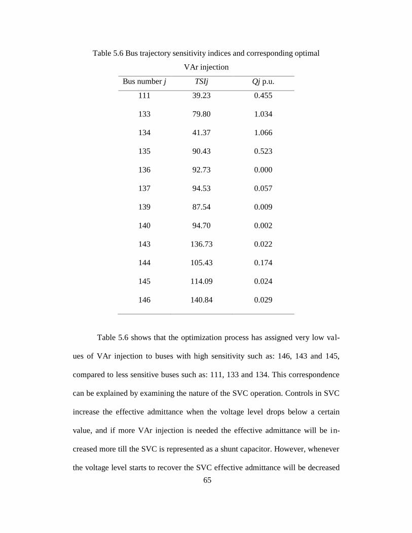
65

Table 5.6 Bus trajectory sensitivity indices and corresponding optimal

VAr injection

Bus number j TSIj Qj p.u.

111 39.23 0.455

133 79.80 1.034

134 41.37 1.066

135 90.43 0.523

136 92.73 0.000

137 94.53 0.057

139 87.54 0.009

140 94.70 0.002

143 136.73 0.022

144 105.43 0.174

145 114.09 0.024

146 140.84 0.029

Table 5.6 shows that the optimization process has assigned very low val-

ues of VAr injection to buses with high sensitivity such as: 146, 143 and 145,

compared to less sensitive buses such as: 111, 133 and 134. This correspondence

can be explained by examining the nature of the SVC operation. Controls in SVC

increase the effective admittance when the voltage level drops below a certain

value, and if more VAr injection is needed the effective admittance will be in-

creased more till the SVC is represented as a shunt capacitor. However, whenever

the voltage level starts to recover the SVC effective admittance will be decreased

66

accordingly to ensure the voltage level stays within an acceptable range. There-

fore, if a large SVC was located at a very sensitive bus, the voltage level of that

bus will need a small amount of VAr injection and will recover very fast, which

will cause the effective admittance of the SVC to drop down to very low values in

a short time. However, if a large SVC was located at a less sensitive bus, the vol-

tage level on that bus will need more time to recover, therefore, the effective ad-

mittance of the SVC will be kept at high levels for longer time, which will cause

more VArs to be injected into the system and therefore increase the voltage mag-

nitudes of other load buses. To illustrate the SVC output with respect to the vol-

tage sensitivity, Figure 5.9 shows the effective admittance (p.u.) for two separate

cases where a 1 p.u. SVC is located on bus 137 (high sensitivity), and on bus 111

(low sensitivity).

67

Figure 5.9 SVC effective admittance with respect to bus sensitivity

5.7 Different Operating Conditions Results

In order to evaluate an optimal set of VAr injection that is valid for differ-

ent operating conditions, the load at the representative load buses was increased to

examine the effect of load growth over the optimal amount of VAr injection

needed. The load was increased by 5%, 10%, 15% and 20%, and for each case the

optimal amount of VAr injection was evaluated. Table 5.7 shows the TSIj for the

VAr injection buses, for each different operating condition.

0 1 2 3 4 5 6 7 8 9 10

0.1

0.2

0.3

0.4

0.5

0.6

0.7

0.8

0.9

1

1.1

Bus 134

Bus 146

SV

C a

dm

itta

nce

(pu)

Time (sec)

68

Table 5.7 Bus trajectory sensitivity indices for different operating conditions

Bus number j

TSIj

Case-1

(5%)

Case-2

(10%)

Case-3

(15%)

Case-4

(20%)

111 31.52 38.56 26.82 26.11

133 53.56 52.47 37.37 35.16

134 28.11 30.21 22.92 22.18

135 56.22 54.83 39.27 36.75

136 76.05 80.00 56.08 44.25

137 78.29 59.34 43.88 40.93

139 74.27 78.24 55.07 43.26

140 78.82 63.73 44.53 41.39

143 116.54 119.57 109.58 100.46

144 92.02 91.07 81.97 68.77

145 90.12 89.77 81.08 77.44

146 125.19 130.88 122.92 111.06

Table 5.7 shows that in general the trajectory sensitivity indices decrease

when the load is increased. However, when the load is increased it is expected

that more VAr injection is needed. This can be concluded from Table 5.8 which

shows the optimal weighted values of VAr injection for each different operating

condition case.

69

Table 5.8 Optimized weighted VAr injection values for different operating

conditions

Bus number j

Qj p.u.

Case-1

(5%)

Case-2

(10%)

Case-3

(15%)

Case-4

(20%)

111 0.502 0.591 0.546 0.584

133 1.079 1.303 1.484 1.486

134 1.280 1.243 1.411 1.506

135 0.694 0.714 0.743 0.821

136 0.000 0.034 0.000 0.000

137 0.072 0.085 0.098 0.114

139 0.021 0.026 0.029 0.060

140 0.017 0.016 0.023 0.054

143 0.033 0.038 0.043 0.059

144 0.194 0.115 0.161 0.153

145 0.030 0.008 0.009 0.010

146 0.035 0.050 0.056 0.061

Total 3.957 4.222 4.605 4.908

In order to compose a final set of VAr injection values that will be valid

for all different operating conditions, the highest value of Qj for each different

operating condition is selected as the choice of the SVC rating for each bus. Table

5.9 shows the VAr injection values for the optimal final set.

70

Table 5.9 Final optimized VAr injection values

Bus number j Qj p.u.

111 0.591

133 1.486

134 1.506

135 0.821

136 0.034

137 0.114

139 0.060

140 0.054

143 0.059

144 0.194

145 0.030

146 0.061

Total 5.011

Figures 5.10-5.11 show the voltage response at low voltage load buses for

case-4 (20% increase in load) without any VAr injection present.

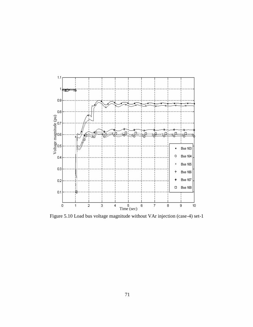
71

Figure 5.10 Load bus voltage magnitude without VAr injection (case-4) set-1

Volt

age

mag

nit

ude

(pu)

Time (sec)

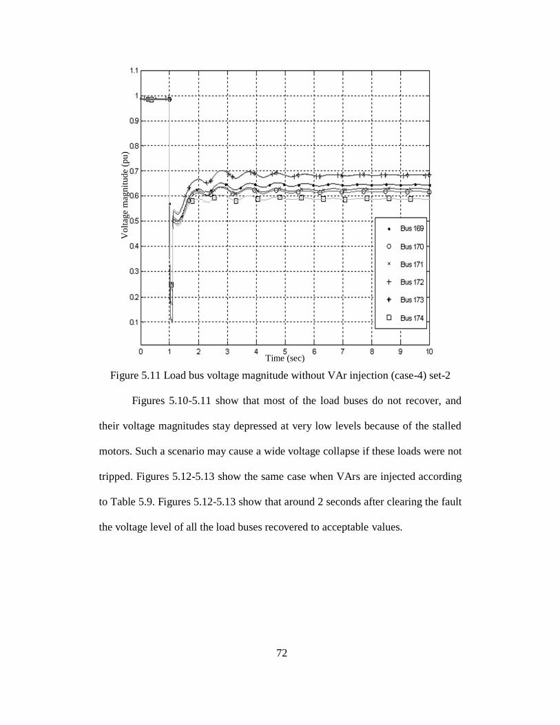
72

Figure 5.11 Load bus voltage magnitude without VAr injection (case-4) set-2

Figures 5.10-5.11 show that most of the load buses do not recover, and

their voltage magnitudes stay depressed at very low levels because of the stalled

motors. Such a scenario may cause a wide voltage collapse if these loads were not

tripped. Figures 5.12-5.13 show the same case when VArs are injected according

to Table 5.9. Figures 5.12-5.13 show that around 2 seconds after clearing the fault

the voltage level of all the load buses recovered to acceptable values.

Volt

age

mag

nit

ude

(pu)

Time (sec)

73

Figure 5.12 Load bus voltage magnitude with final VAr injection values

(case-4) set-1

Volt

age

mag

nit

ude

(pu)

Time (sec)

74

Figure 5.13 Load bus voltage magnitude with final VAr injection values

(case-4) set-2

5.8 A Description of Contingency Results

The optimized final set of VAr injection values should be capable of im-

proving the voltage profile at load buses for a different number of contingencies.

However, since this work used the most severe contingency to evaluate the opti-

mized VAr injection values, the same values were used for the new contingencies.

Therefore, another three 345 kV buses were chosen for the new contingencies;

bus 5, 112 and 128. Figures 5.14-5.15 show the voltage response at low voltage

load buses for contengincy-1 (fault at bus 5), and with 20% load increase, with

final VAr injection set applied.

Volt

age

mag

nit

ude

(pu)

Time (sec)

75

Figure 5.14 Load bus voltage magnitude with final VAr injection values

(fault at bus 5) set-1

Volt

age

mag

nit

ude

(pu)

Time (sec)

76

Figure 5.15 Load bus voltage magnitude with final VAr injection values

(fault at bus 5) set-2

Figures 5.14-5.15 show that this contingency is less severe than the base

case contingency since the voltage level dip during the fault is not as deep as the

base case. The voltage recovery time also is less for this contingency. Figures

5.16-5.17 show the voltage response at low voltage load buses for contengincy-2

(fault at bus 112), and with 20% load increase, with final VAr injection set ap-

plied.

Volt

age

mag

nit

ude

(pu)

Time (sec)

77

Figure 5.16 Load bus voltage magnitude with final VAr injection values

(fault at bus 112) set-1

Time (sec)

Volt

age

mag

nit

ude

(pu)

78

Figure 5.17 Load bus voltage magnitude with final VAr injection values

(fault at bus 112) set-2

In Figures 5.16-5.17, although the voltage dips during the fault are as deep

as it is in the base case, but the voltage recovery time is less for this contingency.

Figures 5.18-5.19 show the voltage response at low voltage load buses for con-

tengincy-2 (fault at bus 128), and with 20% load increase, with final VAr injec-

tion set applied.

Volt

age

mag

nit

ude

(pu)

Time (sec)

79

Figure 5.18 Load bus voltage magnitude with final VAr injection values

(fault at bus 128) set-1

Volt

age

mag

nit

ude

(pu)

Time (sec)

80

Figure 5.19 Load bus voltage magnitude with final VAr injection values

(fault at bus 128) set-2

Figures 5.16 - 5.19 show that the load buses voltage recovery for the dif-

ferent contingencies is very similar to the one of the base case. Actually, it is even

better for some contingencies, since the base contingency is the most severe.

Therefore, the final set of VAr injection values which was evaluated using the op-

timization process is also valid for different contingencies, as well as different

operating conditions.

Volt

age

mag

nit

ude

(pu)

Time (sec)

81

CHAPTER 6

CONCLUSIONS AND FUTURE RESEARCH

6.1 Conclusions

This work examines the voltage instability issue in a power system in the

presence of significant induction motor loads and applies dynamic VAr injection

as a counter-measure to ensure voltage stability following a large disturbance. The

system under study has significant amounts of motor load which causes the vol-

tage response at low voltage buses to be highly nonlinear and discontinuous due

to the dynamic behavior of motors. Therefore, short term voltage instability, in

the form of voltage recovery delay and fast voltage collapse, is considered as the

main threat to overall system stability in this work. Short term voltage instability

issue is exacerbated by single phase low inertia motor loads which represent resi-

dential A/C systems, since they tend to decelerate and stall when their voltage

magnitude drops below a certain level. Motors have an adverse impact on voltage

stability because they consume very large amounts of reactive power within a

very short time during a large disturbance. Therefore, using fast dynamic VAr in-

jection devices was found to be useful in alleviating reactive power deficiency

near load centers throughout this work.

Time domain dynamic analysis was used to evaluate the trajectory voltage

sensitivities which proved their capability of describing voltage response with re-

spect to injected reactive power. Using trajectory voltage sensitivities as weight-

ing factors in the optimization process resulted in assigning an optimum amount

of reactive power injection for each high voltage bus under study, and therefore,

82

determining the optimal SVC size for each bus. The optimization process was al-

so useful in determining the optimal locations for SVCs since some buses were

either not assigned any VAr injection at all, or assigned very small (negligible)

amounts. This work also shows that the optimal amount of VAr injection assigned

for each bus is inversely proportional to the bus voltage sensitivity. This result is

related to the nature of SVC controls operation, and it leads to injecting more

VArs into the system during a large disturbance. Different operating conditions

where the system is more stressed and different contingencies were also inspected

throughout this work to ensure the optimization process robustness and complete-

ness. The final values for SVCs optimal sizes were chosen from different operat-

ing conditions in order to form a worst case scenario set. This final set has im-

proved short term voltage stability when tested on a range of operating conditions

and contingencies.

6.2 Future work

This work considers SVCs as the main dynamic VAr injection device, and

therefore performs the optimization process for determining the required rating of

SVCs. However, since the reactive power output of SVCs is proportional to the

voltage magnitude squared, which is considered a major drawback for SVCs, oth-

er dynamic VAr injection devices such as STATCOMs should be evaluated. Since

the VAr output of STATCOMs is linearly proportional to the voltage magnitude,

it is expected that less VArs would be needed if SVCs were replaced with STAT-

COMs.

83

A range of operating conditions and contingencies were used throughout

this work to evaluate and validate the final optimal VAr injection set. However,

topological changes should also be considered and their effect on voltage sensitiv-

ities should be examined since voltage sensitivities play a major role in the opti-

mization process.

Time domain dynamic analysis is the main tool used in this work to eva-

luate trajectory voltage sensitivities. Therefore, more improved and comprehen-

sive dynamic models should be developed especially for dynamic loads, since the

accuracy of dynamic analysis depends largely on the accuracy of the dynamic

models used.

This work used time domain dynamic simulations and linear optimization

to evaluate the trajectory voltage sensitivities and optimal VAr injection require-

ments quantitatively for a specific power system. The same problem should be

approached analytically using more comprehensive optimization methods such as

Mixed Integer Dynamic Optimization (MIDO), where trajectory voltage sensitivi-

ties would be used among many other constraints. The results of such approaches

should be compared to the results of this study.

84

REFERENCES

[1] B. Lesieutre, D. Kosterev, J. Undrill, “Phasor modeling approach for sin-

gle phase ac motors,” IEEE Power Engineering Society General Meeting, 2008,

pp. 1-7.

[2] P. Kundur, “Power system stability and control,” McGraw Hill, New

York, 1994.

[3] S. Meliopoulos, V. Vittal, J. McCalley, V. Ajjarapu, and I. Hiskens, "Op-

timal allocation of static and dynamic VAr resources,” PSERC Publication,

March 2008.

[4] V.S. Kolluri, and S. Mandal, "Determining reactive power requirements in

the southern part of the entergy system for improving voltage security – A case

study,” IEEE Power System Conference and Exposition, 2006, pp. 119-123.

[5] P. Pourbeik, R. Koessler, W. Quaintance, and W. Wong, "Performing

comprehensive voltage stability studies for the determination of optimal location,

size and type of reactive compensation,” IEEE Power System Conference and Ex-

position, 2006, pp. 118.

[6] IEEE Task Force on Load Representation for Dynamic Performance,

“Load representation for dynamic performance analysis,” IEEE Trans. Power

Systems, 1993, vol. 8, no.2, pp. 472-482.

[7] IEEE Task Force for Load Representation for Dynamic Performance,

“Standard models for power flow and dynamic performance simulation,” IEEE

Trans. Power Systems, 1995, vol. 10, no. 3, pp. 1302-1313.

[8] K. Morison, H. Hamdani, and L. Wang, “Practical issues in load modeling

for voltage stability studies,” IEEE Power Engineering Society General Meeting,

2003, vol. 3, pp. 1392-1397.

[9] D. Kosterev, A. Meklin, J. Undrill, B. Lesieutre, W. Price, D. Chassin, R.

Bravo, and S. Yang, “Load modeling in power system studies: WECC progress

update,” IEEE Power Engineering Society General Meeting, 2008, pp. 1-9.

85

[10] G. K. Stefopoulos and A. P. Meliopoulos, “Induction motor load dynam-

ics: Im-pact on voltage recovery phenomena,” IEEE Power Engineering Society

Transmission and Distribution Conference and Exhibition, 2006, pp. 752-759.

[11] L. Taylor, R. Jones, and S. Halpin, “Development of load models for fault

induced delayed voltage recovery dynamic studies,” IEEE Power and Energy So-

ciety General Meeting, 2008, pp. 1-7.

[12] X. Zheng, R. He, and J. Ma, “A new load model suitable for transient sta-

bility analysis with large voltage disturbances,” Electrical Machines and Systems

(ICEMS), 2010, pp. 1898 – 1902.

[13] K. Rudion, H. Guo, H. Abildgaard, Z. A. Styczynski, "Non-linear load

modeling - requirements and preparation for measurement,” IEEE Power &

Energy Society General Meeting, 2009, pp. 1-7.

[14] V. Stewart and E. H. Camm, “Modeling of stalled motor loads for power

system short term voltage stability analysis,” IEEE Power Engineering Society

General Meeting, 2008, vol. 2, pp. 1887-1892.

[15] P. Pourbeik and B. Agrawal, “A hybrid model for representing air-

conditioner compressor motor behavior in power system studies,” IEEE Power

Engineering Society General Meeting, 2008, pp. 1-8.

[16] B. Sapkota, and V. Vittal, "Dynamic VAr planning in a large power sys-

tem using trajectory sensitivities,” IEEE Transactions on Power Systems, 2010,

pp. 461 – 469.

[17] P. Pourbeik, D. Wang, and K. Hoang, “Load modeling in voltage stability

studies,” Power Engineering Society General Meeting, 2005, pp. 1893 – 1900.

[18] C. Taylor, “Power system voltage stability,” MC Graw Hill, New York,

1994.

86

[19] T. Yong, M. Shiying and Z. Wuzhi, “Mechanism research of short-term

large-disturbance voltage stability,” International Conference on Power System

Technology, 2006, pp. 1-5.

[20] P. Li, B. Zhang, C. Wang, J. Shu, M. You, Y. Wang, Z. Bo, A. Klimek,

“Time-domain simulation investigates short-term voltage stability with dynamic

loads,” Asia-Pacific Power and Energy Engineering Conference, 2009, pp. 1-5.

[21] J. Diaz de Leon II, and C. Taylor, “Understanding and solving short-term

voltage stability problems,” IEEE Power Engineering Society Summer Meeting,

2002, vol. 2, pp. 745 – 752.

[22] C. Sharma, and M. Ganness, "Determination of power system voltage sta-

bility using modal analysis,” International Conference on Power Engineering,

Energy and Electrical Drives, 2007, pp. 381 – 387.

[23] M.Hasani and M.Parniani, "Method of combined static and dynamic anal-

ysis of voltage collapse in voltage stability assessment,” IEEE Transmission

and Distribution Conference and Exhibition: Asia and Pacific, 2005, pp. 1-6.

[24] T. Cutsem, and C. Vournas, “Voltage stability of electric power systems,”

Kluwer Academic Publishers, 1998.

[25] V. Vittal, “Transient stability test systems for direct stability methods,”

IEEE Transactions on Power Systems, 1992, pp. 37-43.

[26] N. Lu, and A. Qiao, “Composite load model evaluation,” Pacific North-

west National Laboratory, September 2007

87