Optimal Insurance with Rank-Dependent Utility and

Increasing Indemnities

Zuo Quan Xu∗ Xun Yu Zhou† Sheng Chao Zhuang‡

April 26, 2016

Abstract

Bernard et al. (2015) study an optimal insurance design problem where an individual’s pref-

erence is of the rank-dependent utility (RDU) type, and show that in general an optimal contract

covers both large and small losses. However, their results suffer from the unrealistic assumption

that the random loss has no atom, as well as a problem of moral hazard for paying more com-

pensation for a smaller loss. This paper addresses these setbacks by removing the non-atomic

assumption, and by exogenously imposing the constraint that both the indemnity function and

the insured’s retention function be increasing with respect to the loss. We characterize the opti-

mal solutions via calculus of variations, and then apply the result to obtain explicitly expressed

contracts for problems with Yaari’s dual criterion and general RDU. Finally, we use numerical

examples to compare the results between ours and that of Bernard et al. (2015).

Keywords: optimal insurance design, rank-dependent utility theory, Yaari’s dual criterion,

probability weighting function, moral hazard, indemnity function, retention function, quantile

formulation.∗Department of Applied Mathematics, The Hong Kong Polytechnic University, Kowloon, Hong Kong. Email:

maxu@polyu.edu.hk. This author acknowledges financial supports from the Hong Kong Early Career Scheme

(No.533112), the Hong Kong General Research Fund (No.529711), the NNSF of China (No.11471276), and the Hong

Kong Polytechnic University.†Mathematical Institute and Nomura Centre for Mathematical Finance, and Oxford–Man Institute of Quantitative

Finance, The University of Oxford, Oxford OX2 6GG, UK. This author acknowledges supports from a start-up fund

of the University of Oxford, and research grants from the Oxford–Nie Financial Big Data Lab, the Nomura Centre

for Mathematical Finance and the Oxford–Man Institute of Quantitative Finance.‡Department of Statistics and Actuarial Science, University of Waterloo, Waterloo, Ontario, N2L 3G1, Canada.

1

1 Introduction

Risk sharing is a method of reducing risk exposure by spreading the burden of loss among several

parties. Mathematically, risk sharing can be generally formulated as a multi-optimization problem in

which a Parato optimality is sought with respect to each party’s well-being modelled as a preference

functional. As such, a risk sharing problem falls naturally into the application domain of operations

research, even though the former has not yet attracted sufficient research interest it deserves in the

community of the latter.

In the context of insurance, the primary risk sharing problem is that of designing an insurance

contract between an insurer and an insured that achieves Parato optimal for the two parties. Specif-

ically, given an upfront premium that the insured pays the insurer, the problem is to determine the

amount of loss I(X) covered by the insurer – called indemnity – for a random, typically nonhedgeable

loss X. The premium usually includes a safety loading on top of the actuarial value of the contract in

order for the insurer to have sufficient incentive to offer the contract - this is called the participation

constraint of the insurer.

Optimal insurance contract design is an important problem, manifested not only in theory but

also in insurance and financial practices. In the insurance literature, most of the work assume that

the insurer is risk neutral1 while the insured is a risk-averse expected utility (EU) maximizer; see

e.g. Arrow (1963), Raviv (1979), and Gollier and Schlesinger (1996). The problem is formulated as

one that maximizes the insured’s expected concave utility function of his net wealth subject to the

insurer’s participant constraint being satisfied. Technically, it is a constrained convex optimization

problem that can be solved by standard optimization techniques. It has been shown in the aforemen-

tioned papers that the optimal contract is in general a deductible one that covers part of the loss in

excess of a deductible level. This theoretical result is consistent with most of the insurance contracts

available in practice. As a result, the problem is reduced to a one-dimensional optimization problem

that determines the optimal deductible. Another important implication of this classical result is that

the insurer and insured shares of risk are both increasing2 functions of the risk; in other words, there

is no incentive for either party to hide risk and thus there is indeed risk sharing.1This assumption is motivated by the fact that an insurer typically has many independent insureds as its clients,

hence its risk is adequately diversified.2Throughout this paper, by an “increasing” function we mean a “non-decreasing” function, namely f is increasing

if f(x) > f(y) whenever x > y. We say f is “strictly increasing” if f(x) > f(y) whenever x > y. Similar conventions

are used for “decreasing” and “strictly decreasing” functions.

2

However, the EU theory has received many criticisms, for it fails to explain numerous experimental

observations and theoretical puzzles. For example, it fails to explain the famous Allais Paradox or

the reason why a same person may buy both lottery and insurance. Other paradoxes/puzzles that

EU theory cannot explain include common ratio effect (Allais, 1953), Friedman and Savage puzzle

(Friedman and Savage, 1948), Ellesberg paradox (Ellesberg, 1961), and the equity premium puzzle

(Mehra and Prescott, 1985). In the context of insurance contracting, the classical EU-based models

again fail to account for some behaviors in insurance demand. Sydnor (2010) investigates how people

choose the deductible decisions between $100, $250, $500, and $1,000. The major finding is that the

households choosing a $500 deductible pay an average premium of $715 per year, yet these households

all rejected a policy with a $1,000 deductible whose average premium was just $615. Since the claim

rate is about 5 percent, effectively these households were willing to pay $100 to protect against a 5

percent possibility of paying an additional $500! As explained by Barberis (2013), this choice can

only be explained by unreasonably high levels of risk aversion within the EU framework. Another

insurance phenomenon that cannot be explained by the EU theory is demand for protection of small

losses (e.g. demand for warranties); see Bernard et al. (2015) for a detailed discussion.

In order to overcome this drawback of the EU theory, different measures of evaluating uncertain

outcomes have been put forward to depict human behaviors. A notable one is the rank-dependent

utility (RDU) proposed by Quiggin (1982). In this theory, the preference measure of a final (random)

wealth W > 0 is defined as

V rdu(W ) =

∫u(W )d(T P) :=

∫R+

u(x)d[−T (1− FW (x))], (1)

where u : R+ 7→ R+ is a (usual) utility function, T : [0, 1] 7→ [0, 1] is called a probability weighting

function, and FW (·) is the cumulative distribution function (CDF) of W . Clearly, if T (x) ≡ x then

V rdu(W ) = E[u(W )], the classical EU. To see what a non-identity function T brings about, we

rewrite assuming that T is differentiable:

V rdu(W ) =

∫R+

u(x)T ′(1− FW (x))dFW (x). (2)

Thus, T ′(1−FW (x)) serves as a weight on the outcome x of W when evaluating the expected utility.

Since this weight depends on 1− FW (x), the decumulative probability or the rank of the outcome x

of W , hence the name of the rank-dependent utility.3 In particular, if T is inverse-S shaped, that is,3On the other hand, the RDU preference reduces to Yaari’s dual criterion (Yaari 1987) when the utility function

is the identity one.

3

it is first concave and then convex; see Figure 1, then T ′(1− FW (x)) > 1 when x is both sufficiently

large and sufficiently small. This captures the common observation that people tend to exaggerate

small probabilities of extremely good and bad outcomes (hence people buy both insurances and

lotteries).

From the optimization point of view, maximizing the RDU preference (1) has a clear challenge:

with the presence of a general weighting function T , (1) is no longer concave even if u is concave.

With the development of advanced mathematical tools, the RDU preference has been applied to

many areas of finance, including portfolio choice and option pricing. In particular, the approach

of the so-called quantile formulation has been developed to deal with the non-convex optimization

involved in solving RDU portfolio choice models (e.g. Jin and Zhou 2008, He and Zhou 2011).

The key idea is to change the decision variable from the wealth W to its quantile function, which

miraculously leads to a concave optimization problem. On the other hand, Barseghyan et al. (2013)

use data on households’ insurance deductible decisions in auto and home insurance to demonstrate

the relevance and importance of the probability weighting and suggest the possibility of generalizing

their conclusions to other insurance choices.

There have been also studies in the area of insurance contract design within the RDU framework;

see for example Chateauneuf, Dana and Tallon (2000), Dana and Scarsini (2007), and Carlier and

Dana (2008). However, all these papers assume that the probability weighting function is convex.

Bernard et al. (2015) are probably the first to study RDU-based insurance contracting with inverse-

S shaped weighting functions, using the quantile formulation. They derive optimal contracts that

not only insure large losses above a deductible level but also cover small ones. However, their results

suffer from two major problems. One is the assumption that the random loss X has no atom, which

is not realistic in the insurance context. The reason is that 0 is typically an atom of X, as it is

plausible that P(X = 0) > 0. The second is that their contracts pose a severe problem of moral

hazard, since they are not increasing with respect to the losses. As a consequence, insureds may be

motivated to hide their true losses in order to obtain additional compensations; see a discussion on

pp. 175–176 of Bernard et al. (2015).

This paper aims to address these setbacks. We consider the same insurance model as in Bernard

et al. (2015), but removing the non-atomic assumption on the loss, and adding an explicit constraint

that both the indemnity function and the insured’s retention function (i.e. the part of the losses to

be born by the insured) must be globally increasing with respect to the losses - this latter constraint

will rule out completely the aforementioned behaviour of moral hazard. However, mathematically

4

we encounter substantial difficulty. The approach used in Bernard et al. (2015) no longer works.

We develop a general approach to overcome this difficulty. Specifically, we first derive the necessary

and sufficient conditions for optimal solutions via calculus of variations. While calculus of variations

is a rather standard technique for infinite-dimensional optimization,4 deducing explicitly expressed

optimal contracts based on these conditions requires a fine and involved analysis. An interesting

finding is that, for a good and reasonable range of parameters specifications, there are only two

types of optimal contracts, one being the classical deductible one and the other a “three-fold" one

covering both small and large losses.

The remainder of the paper is organized as follows. Section 2 presents the optimal insurance

model under the RDU framework including its quantile formulation. Section 3 applies the calculus

of variations to derive a general necessary and sufficient condition for optimal solutions. We then

derive optimal contracts for Yaari’s criterion and the general RDU in Sections 4 and 5, respectively.

Section 6 provides a numerical example to illustrate our results. Finally, we conclude with Section

7. Proofs of some lemmas are placed in an Appendix.

2 The Model

In this section, we present the optimal insurance contracting model in which the insured has the RDU

type of preferences, followed by its quantile formulation that will facilitate deriving the solutions.

2.1 Problem formulation

We follow Bernard et al. (2015) for the problem formulation except for two critical differences, which

we will highlight. Let (Ω,F,P) be a probability space. An insured, endowed with an initial wealth

W0, faces a non-negative random loss X, possibly having atoms and supported in [0,M ], where M is

a given positive scalar. He chooses an insurance contract to protect himself from the loss, by paying

a premium π to the insurer in return for a compensation (or indemnity) in the case of a loss. This

compensation is to be determined as a function of the loss X, denoted by I(·) throughout this paper.

The retention function R(X) := X− I(X) is thereby the part of the loss to be borne by the insured.4Calculus of variations has also been applied in the insurance context. For example, Spence and Zeckhauser (1971)

employ calculus of variations to solve an insurance contracting problem in the setting of expected utility theory. Yong

and Browne (1997) apply calculus of variations to determine equilibrium insurance policies under adverse selection

within, again, the expected utility framework.

5

For a given X, the insured aims to choose an insurance contract that provides the best tradeoff

between the premium and compensation based on his risk preference. In this paper, we consider the

case when insured’s preference on the final random wealth W > 0 is dictated by the RDU functional

(1), where u : R+ 7→ R+ and T : [0, 1] 7→ [0, 1]. On the other hand, if the insurer is risk-neutral and

the cost of offering the compensation is proportional to the expectation of the indemnity, then the

premium to be charged for an insurance contract should satisfy the participation constraint

π > (1 + ρ)E[I(X)],

where the constant ρ is the safety loading of the insurer.

It is natural to require an indemnity function to satisfy

I(0) = 0, 0 6 I(x) 6 x, ∀ 0 6 x 6 M, (3)

a constraint that has been imposed in most insurance contracting literature. If the insured’s pref-

erence is dictated by the classical EU theory, then the optimal contract is typically a deductible

contract which automatically renders the indemnity function increasing; see e.g. Arrow (1971) and

Raviv (1979). However, for the RDU preference the resulting optimal indemnity may not be an

increasing function, as shown in Bernard et al. (2015). This may potentially cause moral hazard as

pointed out earlier. Similarly, a non-monotone retention function may also lead to moral hazard. To

incoperate the increasing constraint on the contract has been an outstanding open question.

In this paper, we require both the indemnity function and the retention function to be globally

increasing. Economically speaking, this means the insurer and insured wealths are comonotone, both

bearing more when a bigger loss happens. Mathematically speaking, we require

I(y) 6 I(x), R(y) 6 R(x), ∀ 0 6 y 6 x 6 M. (4)

As R(x) ≡ x − I(x), it is easily seen that the joint constraint of (3) and (4) is equivalent to the

following one

I(0) = 0, 0 6 I(x)− I(y) 6 x− y, ∀ 0 6 y 6 x 6 M. (5)

We can now formulate our insurance contracting problem as

maxI(·)

V rdu(W0 − π −X + I(X))

s.t. (1 + ρ)E[I(X)] 6 π,

I(·) ∈ I,

(6)

6

where

I := I(·) : I(0) = 0, 0 6 I(x)− I(y) 6 x− y, ∀ 0 6 y 6 x 6 M, (7)

and W0 and π are fixed scalars.

For any random variable Y > 0 a.s., define the quantile function of Y as

F−1Y (t) := infx ∈ R+ : P (Y 6 x) > t, t ∈ [0, 1].

Note that any quantile function is nonnegative, increasing and left-continuous (ILC).

We now introduce the following assumptions that will be used hereafter.

Assumption 2.1 The random loss X has a strictly increasing distribution function FX . Moreover,

F−1X is absolutely continuous on [0, 1].

Assumption 2.2 (Concave Utility) The utility function u : R+ 7→ R+ is strictly increasing and

continuously differentiable. Furthermore, u′ is decreasing.

Assumption 2.3 (Inverse-S Shaped Weighting) The probability weighting function T is a continu-

ous and strictly increasing mapping from [0,1] onto [0,1] and twice differentiable on (0, 1). Moreover,

there exists b ∈ (0, 1) such that T ′(·) is strictly decreasing on (0, b) and strictly increasing on (b, 1).

Furthermore, T ′(0+) := limz↓0 T′(z) > 1 and T ′(1−) := limz↑1 T

′(z) = +∞.

The first part of Assumption 2.1, crucial for the quantile formulation, is standard; see e.g. Raviv

(1979). As noted, a significant difference from Bernard et al. (2015) is that here we allow X to have

atoms. For example, let FX(x) = 1−γe−ηx

1−γe−ηM for x ∈ [0,M ], where γ ∈ (0, 1) and η > 0. Then, X

satisfies Assumption 2.1, and has an atom at 0 with the probability P(X = 0) = 1−γ1−γe−ηM > 0. This

assumption also ensures that F−1X (FX(x)) ≡ x,∀ x ∈ [0,M ], a fact that will be used often in the

subsequent analysis. Next, Assumption 2.2 is standard for a utility function. Finally, Assumption

2.3 is satisfied for many weighting functions proposed or used in the literature, e.g. the one proposed

by Tversky and Kahneman (1992) (parameterized by θ):

Tθ(x) =xθ

(xθ + (1− x)θ)1θ

. (8)

Figure 1 displays this (inverse-S shaped) weighting function (in blue) when θ = 0.5.

In practice, most of the insurance contracts are not tailor-made for individual customers. Instead,

an insurance company usually has contracts with different premiums to accommodate customers

7

0 0.2 0.4 0.6 0.8 10

0.1

0.2

0.3

0.4

0.5

0.6

0.7

0.8

0.9

1

x

T(x

)

a c

Figure 1: An inverse-S shaped weighting function (in blue) satisfying Assumption 2.3. The marked

points a and c will be explained later.

with different needs. Each contract is designed with the best interest of a representative customer

in mind so as to stay marketable and competitive, while maintaining the desired profitability (the

participation constraint). An insured can then choose one from the menu of contracts to cater for

individual needs. The problem (6) is therefore motivated by the insurer’s making of this menu.

If the premium π > (1 + ρ)E[X], then I∗(x) ≡ x (corresponding to a full coverage) is feasible

and maximizes the objective function in the problem (6) pointwisely; hence optimal. To rule out

this trivial case, henceforth we restrict 0 < π < (1 + ρ)E[X]. Moreover, we assume

W0 − (1 + ρ)E[X]−M > 0, (9)

to ensure that the policyholder will not go bankrupt because W0 − π − M > 0 for all 0 < π <

(1 + ρ)E[X].

It is more convenient to consider the retention function R(x) = x − I(x) instead of I(x) in our

study below. Letting

∆ : = E[X]− π

1 + ρ∈ (0, E[X]),

W : = W0 − (1 + ρ)E[X] > 0,

W∆ : = W + (1 + ρ)∆ ≡ W0 − π,

8

one can easily reformulate (6) in terms of R(·):

maxR(·)

V rdu(W∆ −R(X))

s.t. E[R(X)] > ∆,

R(·) ∈ R,

(10)

where

R := R(·) : R(0) = 0, 0 6 R(x)−R(y) 6 x− y, ∀ 0 6 y 6 x 6 M.

2.2 Quantile Formulation

The objective function in (10) is not concave in R(X) (due to the nonlinear weighting function T ),

leading to a major difficulty in solving (10). However, under Assumption 2.3, we have

V rdu(W∆ −R(X)) =

∫R+

u(x)d[−T (1− FW∆−R(X)(x))]

=

∫ 1

0

u(F−1W∆−R(X)(z))T

′(1− z)dz =

∫ 1

0

u(W∆ − F−1R(X)(1− z))T ′(1− z)dz

=

∫ 1

0

u(W∆ − F−1R(X)(z))T

′(z)dz,

where the third equality is because

F−1W∆−R(X)(z) = W∆ − F−1

R(X)(1− z)

except for an at most countable set of z. Moreover, E[R(X)] > ∆ is equivalent to∫ 1

0F−1R(X)(z)dz > ∆.

The above suggests that we may change the decision variable from the random variable R(X) to

its quantile function F−1R(X), with which the objective function of (10) becomes concave and the first

constraint is linear. It remains to rewrite the monotonicity constraint (represented by the constraint

set R) also in terms of F−1R(X). To this end, the next lemma plays an important role.

Lemma 2.1 Under Assumption 2.1, for any given R(·) ∈ R, we have

R(x) = F−1R(X)(FX(x)), ∀ x ∈ [0,M ].

Proof: First, by the monotonicity of R(·), we have

P(R(X) 6 R(x)) > P(X 6 x) = FX(x),

so by the definition of F−1R(X)(FX(x)), we conclude that

F−1R(X)(FX(x)) 6 R(x).

It suffices to prove the reverse inequality. There are two possible cases.

9

• R(x) = 0. In this case, we have F−1R(X)(FX(x)) = 0 as quantile functions are always nonnegative

by definition.

• R(x) > 0. It suffices to prove that P(R(X) 6 z) < FX(x) for any z < R(x). Take z1 such

that z < z1 < R(x). By the continuity and monotonicity of R(·), there exists y < x such that

R(y) = z1. Then,

P(R(X) 6 z) 6 P(R(X) < z1) = P(R(X) < R(y)) 6 P(X 6 y) = FX(y) < FX(x),

where we have used the fact that FX is strictly increasing under Assumption 2.1.

The claim is thus proved.

In view of the above results, we can rewrite (10) as the following problem, in which the decision

variable is F−1R(X)(·) (denoted by G(·) for simplicity):

maxG(·)

∫ 1

0u(W∆ −G(z))T ′(z)dz,

s.t.∫ 1

0G(z)dz > ∆,

G(·) ∈ G,

(11)

where G := F−1R(X)(·) : R(·) ∈ R.

In the absence of an explicit expression the constraint set G is hard to deal with. The following

result addresses this issue. Note the major technical difficulty arises from the possible existence of

the atoms of X.

Lemma 2.2 Under Assumption 2.1, we have

G = G(·) : G(·) is absolutely continuous, G(0) = 0, 0 6 G′(z) 6 (F−1X )′(z), a.e. z ∈ [0, 1]. (12)

Proof: We denote the right hand side of (12) by G1. For any G(·) ∈ G, there exists R(·) ∈ R

such that G(·) = F−1R(X)(·). For any 0 6 b < a 6 1, define

a = infx ∈ [0,M ] : R(x) = G(a),

a = supx ∈ [0,M ] : R(x) = G(a),

define b and b similarly. Let us show that a 6 F−1X (a) 6 a. In fact, by definition,

F−1X (a) = infx ∈ R+ : FX(x) > a > infx ∈ R+ : G(FX(x)) > G(a)

10

= infx ∈ R+ : R(x) > G(a) = a.

Suppose F−1X (a)− ε > a for some ε > 0. Then by monotonicity,

G(a) = R(a) < R(F−1X (a)− ε) = G(FX(F

−1X (a)− ε)) 6 G(a),

where we have used the fact that FX(F−1X (a) − ε) < a to get the last inequality. This leads to a

contradiction; hence it must hold that F−1X (a) 6 a. Similarly, we can prove b 6 F−1

X (b) 6 b. Then

we have

0 6 G(a)−G(b) = R(a)−R(b) 6 a− b 6 F−1X (a)− F−1

X (b).

This inequality shows that G is absolutely continuous since F−1X is an absolutely continuous function

under Assumption 2.1. Furthermore, it also implies

0 6 G′(z) 6 (F−1X )′(z),

a.e. z ∈ [0, 1]. So we have established that G ⊆ G1.

To prove the reverse inclusion, take any G(·) ∈ G1 and define R(·) = G(FX(·)). It follows from

Assumption 2.1 that

0 6 R(0) = G(FX(0))−G(0) 6 F−1X (FX(0))− F−1

X (0) = 0

and

0 6 R(a)−R(b) = G(FX(a))−G(FX(b)) 6 F−1X (FX(a))− F−1

X (FX(b)) = a− b, ∀ 0 6 b < a 6 1.

Hence R(·) ∈ R. It now suffices to show G(a) = F−1R(X)(a) for any 0 6 a 6 1. If G(a) = 0,

then G(a) 6 F−1R(X)(a) holds. Otherwise, for any s < G(a), there exists y such that s < R(y) =

G(FX(y)) < G(a) by the continuity of R(·). Then by the monotonicity of R(·) and G(·), we have

P(R(X) 6 s) 6 P(R(X) < R(y)) 6 P(X 6 y) = FX(y) < a,

which means G(a) 6 F−1R(X)(a). Using the same notation, a, as above, and noting that G(a) =

R(a) = G(FX(a)), we have a 6 FX(a) by the definition of a and the continuity of R(·). Moreover,

it follows from

P(R(X) 6 G(a)) = P(R(X) 6 R(a)) = P(X 6 a) = FX(a)

that F−1R(X)(FX(a)) 6 G(a). Therefore,

G(a) 6 F−1R(X)(a) 6 F−1

R(X)(FX(a)) 6 G(a)

11

holds by monotonicity. The desired result follows.

To solve (11), we apply the Lagrange dual method to remove the constraint∫ 1

0G(z)dz −∆ > 0

and consider the following auxiliary problem:

maxG(·)

U∆(λ,G(·)) :=∫ 1

0[u(W∆ −G(z))T ′(z) + λG(z)]dz − λ∆,

s.t. G(·) ∈ G.(13)

The existence of the optimal solutions to (11) and (13) (for each given λ ∈ R+) is established in

Appendix B, while the uniqueness is straightforward when the utility function u is strictly concave.

To derive the optimal solution to (11), we first solve (13) to obtain an optimal solution, denoted by

Gλ(·). Then we determine λ∗ ∈ R+ by binding the constraint∫ 1

0Gλ∗(z)dz = ∆. A standard duality

argument then deduces that G∗(·) := Gλ∗(·) is an optimal solution to (11). Finally, an optimal

solution to (10) is given by R∗(z) = G∗(FX(z)) ∀z ∈ [0,M ] and that to (6) by I∗(z) = z − R∗(z)

∀z ∈ [0,M ].

So our problem boils down to solving (13). However, in doing so the convex constraint that

0 6 G′(z) 6 (F−1X )′(z) in G poses the major difficulty compared with Bernard et al. (2015) in which

the constraint is a convex cone.

3 Characterization of Solutions

In this section, we derive a necessary and sufficient condition for a function to be optimal to (13).

Assume Gλ(·) solves (13) with a fixed λ. Let G(·) ∈ G be arbitrary and fixed. For any ε ∈ (0, 1),

set Gϵ(·) = (1 − ϵ)Gλ(·) + ϵG(·). Then Gϵ(·) ∈ G. By the optimality of Gλ(·) and the concavity of

u, we have

0 > 1

ε

∫ 1

0

[u(W∆ −Gϵ(z))T ′(z) + λGϵ(z)] dz −∫ 1

0

[u(W∆ − Gλ(z))T

′(z) + λGλ(z)]dz

=

1

ε

∫ 1

0

[(u(W∆ −Gϵ(z))− u(W∆ − Gλ(z)))T

′(z) + λ(Gϵ(z)− Gλ(z))]dz

> 1

ε

∫ 1

0

[(u′(W∆ −Gϵ(z)))(W∆ −Gϵ(z)−W∆ + Gλ(z))T

′(z) + λ(Gϵ(z)− Gλ(z))]dz

ϵ ↓ 0−−→

∫ 1

0

[(u′(W∆ − Gλ(z)))(Gλ(z)−G(z))T ′(z) + λ(G(z)− Gλ(z))

]dz

=

∫ 1

0

[u′(W∆ − Gλ(z))T

′(z)− λ](Gλ(z)−G(z))dz. (14)

12

Define

Nλ(z) := −∫ 1

z

[u′(W∆ − Gλ(t))T

′(t)− λ]dt, z ∈ [0, 1]. (15)

Then (14) yields

0 >∫ 1

0

[u′(W∆ − Gλ(z))T

′(z)− λ](Gλ(z)−G(z))dz =

∫ 1

0

∫ z

0

(G′λ(t)−G′(t))dtdNλ(z)

=

∫ 1

0

∫ 1

t

(G′λ(t)−G′(t))dNλ(z)dt =

∫ 1

0

Nλ(t)(G′(t)− G′

λ(t))dt,

leading to ∫ 1

0

Nλ(z)G′(z)dz 6

∫ 1

0

Nλ(z)G′λ(z)dz, ∀ G(·) ∈ G.

In other words, G′λ(·) maximizes

∫ 1

0Nλ(z)G

′(z)dz over G(·) ∈ G. Therefore, a necessary condition

for Gλ(·) to be optimal for (13) is

G′λ(z)

a.e.=

0, if Nλ(z) =

∫ 1

z[λ− u′(W∆ − Gλ(t))T

′(t)]dt < 0,

∈ [0, (F−1X )′(z)], if Nλ(z) =

∫ 1

z[λ− u′(W∆ − Gλ(t))T

′(t)]dt = 0,

(F−1X )′(z), if Nλ(z) =

∫ 1

z[λ− u′(W∆ − Gλ(t))T

′(t)]dt > 0.

(16)

It turns out that (16) completely characterizes the optimal solutions to (13).

Theorem 3.1 A function Gλ(·) is an optimal solution to (13) if and only if Gλ(·) ∈ G and Gλ(·)

satisfies (16).

Proof: We only need to prove the "if" part. For any feasible G(·) in G, we have

U∆(λ, Gλ(·))− U∆(λ,G(·))

=

∫ 1

0

[u(W∆ − Gλ(z))− u(W∆ −G(z))]T ′(z)dz +

∫ 1

0

λ(Gλ(z)−G(z))dz

>∫ 1

0

u′(W∆ − Gλ(z))(G(z)− Gλ(z))T′(z)dz −

∫ 1

0

λ(G(z)− Gλ(z))dz

=

∫ 1

0

N ′λ(z)(G(z)− Gλ(z))dz =

∫ 1

0

Nλ(t)(G′λ(t)−G′(t))dt > 0.

Hence, Gλ(·) is optimal for (13).

The above theorem establishes a general characterization result for the optimal solutions of (13).

This result, however, is only implicit as an optimal Gλ(·) appears on both sides of (16). Moreover,

the derivative of Gλ(z) is undetermined when Nλ(z) = 0. In the next two sections, we will apply

this general result to derive the solutions.

13

4 Model with Yaari’s Dual Criterion

When u(x) ≡ x, the corresponding V rdu reduces to the so-called Yaari’s dual criterion (Yaari 1987).

In this section we solve our insurance problem with Yaari’s criterion by applying Theorem 3.1. In

this case, the condition (16) is greatly simplified.

Indeed, when u(x) ≡ x, (16) reduces to

G′λ(z)

a.e.=

0, if

∫ 1

z(λ− T ′(t))dt = λ(1− z)− (1− T (z)) < 0,

∈ [0, (F−1X )′(z)], if

∫ 1

z(λ− T ′(t))dt = λ(1− z)− (1− T (z)) = 0,

(F−1X )′(z), if

∫ 1

z(λ− T ′(t))dt = λ(1− z)− (1− T (z)) > 0.

(17)

It should be noted that although u(x) ≡ x is not strictly concave here, the uniqueness of optimal

solution to (13) is implied by the characterizing condition (17).

To apply (17), we need to compare λ and 1−T (z)1−z

. Define

f(z) :=1− T (z)

1− z, z ∈ [0, 1).

Lemma 4.1 The function f(·) is a continuous function on [0, 1). Moreover, under Assumption 2.3,

there exists a unique a ∈ (0, b) such that f(·) is strictly decreasing on [0, a] and strictly increasing on

[a, 1).

Proof: We have

f ′(z) =(1− T (z))− T ′(z)(1− z)

(1− z)2=

p(z)

(1− z)2,

where

p(z) := (1− T (z))− T ′(z)(1− z).

Since

p′(z) = −T ′(z) + T ′(z)− T ′′(z)(1− z) = −T ′′(z)(1− z),

it follows from Assumption 2.3 that p′(z) > 0 for z ∈ (0, b) and p′(z) < 0 for z ∈ (b, 1). Moreover,

p(0+) = 1− T ′(0+) < 0,

p(b) = (1− T (b))− T ′(b)(1− b) =

(1− T (b)

1− b− T ′(b)

)(1− b) > 0,

and

p(1−) = limz↑1

(1− T (z)

1− z− T ′(z)

)(1− z) > 0,

14

as T (·) is strictly convex on [b, 1]. So, there exists a ∈ (0, b) such that p(z) < 0 for z ∈ [0, a) and

p(z) > 0 for z ∈ (a, 1). The desired result follows.

Clearly, f(0) = 1, f(1−) = +∞. Let a be defined as in Lemma 4.1. From the proof of Lemma

4.1, it is easily seen that a is uniquely determined by

T ′(a) =1− T (a)

1− a. (18)

Set

λ := f(a) < f(0) = 1.

Let c ∈ (a, 1] be the unique scalar such that f(c) = 1, or equivalently, T (c) = c. See Figure 1 for the

locations of the points a and c.

Now, we proceed by considering three cases based on the value of λ.

Case I λ 6 λ. In this case,

Nλ(z) = (1− z)(λ− f(z)) < 0 ∀z ∈ [0, a) ∪ (a, 1].

It then follows from (17) that G′λ(z)

a.e.= 0; hence Gλ(z) = 0 ∀ z ∈ [0, 1]. Thus the corresponding

retention Rλ(z) = 0 ∀z ∈ [0,M ] and indemnity Iλ(z) = z ∀z ∈ [0,M ], namely, the optimal

contract is a full insurance contract.

Case II λ < λ < 1. By Lemma 4.1, there exist unique x0 ∈ (0, a) and y0 ∈ (a, c) such that f(x0) =

f(y0) = λ. Accordingly, we have

Nλ(z) =

< 0, if 0 < z < x0,

> 0, if x0 < z < y0,

< 0, if y0 < z < 1.

Hence, (17) leads to the following function:

Gλ(z) =

0, if 0 6 z < x0,

F−1X (z)− F−1

X (x0), if x0 6 z < y0,

F−1X (y0)− F−1

X (x0), if y0 6 z 6 1.

(19)

15

The corresponding retention and indemnity functions are, respectively,

Rλ(z) ≡ Gλ(FX(z)) =

0, if 0 6 z < F−1

X (x0),

z − F−1X (x0), if F−1

X (x0) 6 z < F−1X (y0),

F−1X (y0)− F−1

X (x0), if F−1X (y0) 6 z 6 M,

and

Iλ(z) ≡ z − Rλ(z) =

z, if 0 6 z < F−1

X (x0),

F−1X (x0), if F−1

X (x0) 6 z < F−1X (y0),

z − F−1X (y0) + F−1

X (x0), if F−1X (y0) 6 z 6 M.

(20)

The corresponding indemnity function is schematically illustrated by Figure 2. Qualitatively,

the insurance covers not only large losses (when z > F−1X (y0)) but also small losses (when

z < F−1X (x0)), and the compensation is a constant for the median range of losses. We term

such a contract a threefold one. The need for small loss coverage along with its connection to

the probability weighting are amply discussed in Bernard et al. (2015). However, in Bernard

et al. (2015) the optimal indemnity is strictly decreasing in some ranges of the losses. Such a

contract may incentivize the insured to hide partial losses in order to get more compensations.

In contrast, both our indemnity and retention are increasing functions of the loss, which will

rule out this sort of moral hazard.

Case III 1 6 λ < +∞. By Lemma 4.1, there exists a unique z0 ∈ [c, 1] such that f(z0) = λ. Thus

Nλ(z) =

> 0, if 0 < z < z0,

< 0, if z0 < z < 1.

By (17), we have

Gλ(z) =

F−1X (z), if 0 6 z < z0,

F−1X (z0), if z0 6 z 6 1.

(21)

So

Iλ(z) ≡ z − Rλ(z) =

0, if 0 6 z < F−1X (z0),

z − F−1X (z0), if F−1

X (z0) 6 z 6 M.

(22)

This contract is a standard deductible contract in which only losses above a deductible point

will be covered.

16

Loss X

Inde

mni

ty I(

X)

M

Figure 2: A schematic illustration of a threefold contract: it covers small losses as well as large losses

in excess of a deductible.

Define

G(z) =

F−1X (z), if 0 6 z < c,

F−1X (c), if c 6 z 6 1,

(23)

and let

Kc :=

∫ 1

0

G(z)dz,

and

πc := (1 + ρ)(E[X]−Kc).

Clearly Kc 6∫ 1

0F−1X (z)dz = E[X].

We are now in the position to state our main result in terms of the premium π and the indemnity

function I(·).

Theorem 4.2 Under Yaari’s criterion, u(x) ≡ x, and Assumptions 2.1 and 2.3, the optimal in-

demnity function I∗(·) to the problem (6) is given as

(i) If π = (1 + ρ)E[X], then I∗(z) = z ∀z ∈ [0,M ].

17

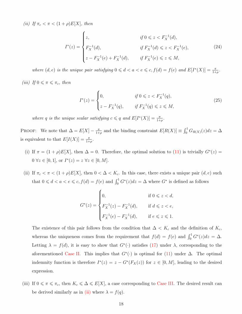
(ii) If πc < π < (1 + ρ)E[X], then

I∗(z) =

z, if 0 6 z < F−1

X (d),

F−1X (d), if F−1

X (d) 6 z < F−1X (e),

z − F−1X (e) + F−1

X (d), if F−1X (e) 6 z 6 M,

(24)

where (d, e) is the unique pair satisfying 0 6 d < a < e 6 c, f(d) = f(e) and E[I∗(X)] = π1+ρ

.

(iii) If 0 6 π 6 πc, then

I∗(z) =

0, if 0 6 z < F−1X (q),

z − F−1X (q), if F−1

X (q) 6 z 6 M,

(25)

where q is the unique scalar satisfying c 6 q and E[I∗(X)] = π1+ρ

.

Proof: We note that ∆ = E[X]− π1+ρ

and the binding constraint E[R(X)] ≡∫ 1

0GR(X)(z)dz = ∆

is equivalent to that E[I(X)] = π1+ρ

.

(i) If π = (1 + ρ)E[X], then ∆ = 0. Therefore, the optimal solution to (11) is trivially G∗(z) =

0 ∀z ∈ [0, 1], or I∗(z) = z ∀z ∈ [0,M ].

(ii) If πc < π < (1 + ρ)E[X], then 0 < ∆ < Kc. In this case, there exists a unique pair (d, e) such

that 0 6 d < a < e 6 c, f(d) = f(e) and∫ 1

0G∗(z)dz = ∆ where G∗ is defined as follows

G∗(z) =

0, if 0 6 z < d,

F−1X (z)− F−1

X (d), if d 6 z < e,

F−1X (e)− F−1

X (d), if e 6 z 6 1.

The existence of this pair follows from the condition that ∆ < Kc and the definition of Kc,

whereas the uniqueness comes from the requirement that f(d) = f(e) and∫ 1

0G∗(z)dz = ∆.

Letting λ = f(d), it is easy to show that G∗(·) satisfies (17) under λ, corresponding to the

aforementioned Case II. This implies that G∗(·) is optimal for (11) under ∆. The optimal

indemnity function is therefore I∗(z) = z − G∗(FX(z)) for z ∈ [0,M ], leading to the desired

expression.

(iii) If 0 6 π 6 πc, then Kc 6 ∆ 6 E[X], a case corresponding to Case III. The desired result can

be derived similarly as in (ii) where λ = f(q).

18

The proof is completed.

The economic interpretation of this result is clear. When the premium is small (0 6 π 6 πc), the

contract only compensates large losses in excess of certain amount. When the premium is in middle

range (πc < π < (1 + ρ)E[X]), the contract is a threefold one, covering both small and large losses.

When the premium is sufficiently large (π > (1 + ρ)E[X]), it is a full coverage.

It is interesting to investigate the comparative statics of the point πc (in terms of c) that triggers

the coverage for small losses. In fact, as

Kc =

∫ c

0

F−1X (z)dz + F−1

X (c)(1− c),

we have∂Kc

∂c= (1− c)(F−1

X )′(c).

However, πc = (1 + ρ)(E[X]−Kc); hence

∂πc

∂c= (1 + ρ)(c− 1)(F−1

X )′(c) < 0.

This implies that the insurer is more willing to be protected against small losses if his weighting

function has a bigger c. This is consistent with the fact that a bigger c renders a larger concave

domain of the probability weighting that overweighs small losses (refer to Figure 1).

5 Model with the RDU Criterion

In this section we study the general RDU model in which the utility function is strictly concave.

Compared with the Yaari model, solving the corresponding insurance problem calls for a more

delicate analysis.

For any twice differentiable function f with f ′(x) = 0, define its Arrow-Pratt measure of absolute

risk aversion

Af (x) := −f ′′(x)

f ′(x).

We now introduce the following assumptions.

Assumption 5.1 (Strictly Concave Utility) The utility function u : R+ 7→ R+ is strictly increasing

and twice differentiable. Furthermore, u′ is strictly decreasing.

19

Assumption 5.2 (i) The function Au(z) is decreasing on (0,∞).

(ii) AT (z) > Au(W − F−1X (z))(F−1

X )′(z), ∀z ∈ (0, a].

Assumption 5.1 is to replace Assumption 2.2, ensuring a genuine RDU criterion. Assumption

5.2-(i) requires that the absolute risk aversion measure of the utility function u is decreasing, which

holds true for many frequently used utility functions including logarithmic, power and exponential

utilities. In general, experimental and empirical evidences are consistent with the decreasing absolute

risk aversion; see e.g. Friend and Blume (1975). On the other hand, AT (z), z ∈ (0, a], measures the

level of probability weighting for small losses. The economical interpretation of Assumption 5.2-(ii)

is, therefore, that the degree of the insured’s concern for small losses is sufficiently large relative to the

absolute risk aversion of the utility function. Note that Assumption 5.2-(ii) is automatically satisfied

when F−1X (z) = 0, ∀z ∈ [0, a], which is equivalent to P(X = 0) > a. In practice, P(X = 0) > 0.5 is a

plausible assumption for many insurance products such as automobile and house insurance. On the

other hand, a is very small for many commonly used inverse-S shaped weighting functions. Take

Tversky and Kahneman’s weighting function (8) as an example, a ≈ 0.013 when θ = 0.3, a ≈ 0.07

when θ = 0.5, and a ≈ 0.166 when θ = 0.8. In these cases, Assumption 5.2-(ii) holds automatically.

The problem (11) has trivial solutions in the following two cases. When ∆ = 0, the optimal

solution is G∗(z) = 0 ∀z ∈ [0, 1], corresponding to a full coverage. When ∆ = E[X], the optimal

solution is G∗(z) = F−1X (z) ∀z ∈ [0, 1] as it is the only feasible solution, corresponding to no coverage.

So we are interested in only the case 0 < ∆ < E[X]. It follows from Proposition C.1 in Appendix

C that there exists λ∗ such that Gλ∗(·) is optimal solution to (13) under λ∗ and∫ 1

0Gλ∗(z)dz = ∆.

Furthermore, recall that we have proved that (13) has a unique solution when u is strictly concave

and (16) provides the necessary and sufficient condition for the optimal solution.

Lemma 5.1 For any G(·) ∈ G, if there exists z ∈ (0, 1) such that

λ− u′(W∆ −G(z))T ′(z) =

∫ 1

z

[λ− u′(W∆ −G(t))T ′(t)]dt = 0,

then z 6 a.

Proof: From λ− u′(W∆ −G(z))T ′(z) = 0, it follows

u′(W∆ −G(z)) =λ

T ′(z).

20

Hence, if z > a, then

0 =

∫ 1

z

[λ− u′(W∆ −G(t))T ′(t)] dt

6∫ 1

z

[λ− u′(W∆ −G(z))T ′(t)] dt =λ

T ′(z)(1− z)

[T ′(z)− 1− T (z)

1− z

]< 0,

where the last inequality is due to Lemma A.1-(i) in Appendix A. This is a contradiction.

Lemma 5.2 Under Assumption 5.2, for any G(·) ∈ G, u′(W∆ −G(z))T ′(z) is a strictly decreasing

function of z on [0, a].

Proof: Noting W∆ > W , it follows from Assumption 5.2 that

AT (z) > Au(W − F−1X (z))(F−1

X )′(z) > Au(W∆ − F−1X (z))(F−1

X )′(z), ∀z ∈ (0, a].

This leads to

d

dz(u′(W∆ −G(z))T ′(z))

= u′(W∆ −G(z))T ′(z) [Au(W∆ −G(z))G′(z)− AT (z)]

< u′(W∆ −G(z))T ′(z)[Au(W∆ −G(z))(F−1

X )′(z)− Au(W∆ − F−1X (z))(F−1

X )′(z)]

= u′(W∆ −G(z))T ′(z)[Au(W∆ −G(z))− Au(W∆ − F−1

X (z))](F−1

X )′(z)

6 0,

where the last inequality is due to the fact that Au is decreasing and G(z) 6 F−1X (z). The proof is

complete.

Now, for any λ 6 λu′(W∆), we have∫ 1

z

[λ− u′(W∆ − Gλ(t))T

′(t)]dt 6

∫ 1

z

[λu′(W∆)− u′(W∆)T

′(t)]dt

= u′(W∆)

∫ 1

z

[λ− T ′(t)]dt = u′(W∆)(1− z)

[λ− 1− T (z)

1− z

]< 0,

where the last inequality is due to Lemma 4.1. Hence Gλ(z) = 0 ∀z ∈ [0, 1] is the only solution

satisfying (16). However,∫ 1

0Gλ(z)dz = 0 < ∆, a contradiction. Therefore, only when λ > λu′(W∆)

it is possible for (16) to hold.

21

Fixing λ > λu′(W∆), we now analyze the shape of the function Gλ(·) that satisfies (16). Suppose

that Gλ(1) = k < W∆. We then have Nλ(1) = 0 and λ−u′(W∆−k)T ′(1−) < 0 since T ′(1−) = +∞.

So, G′λ(z) = 0 when z is close to 1 since Nλ(z) < 0 for such z. Hence, Gλ(z) ≡ k ∀z ∈ [z1, 1] for

some z1 ∈ [0, 1), at which Nλ(z1) = 0 and Nλ(z) < 0 for ∀z ∈ (z1, 1). Next, we consider three cases

respectively depending on the value of k and location of z1.

Case (A) k > W∆ − (u′)−1(λλ), i.e. λ < λu′(W∆ − k). In this case, we have, for any z ∈ [0, 1),∫ 1

z

[λ− u′(W∆ − k)T ′(t)] dt <

∫ 1

z

[λu′(W∆ − k)− u′(W∆ − k)T ′(t)

]dt

= u′(W∆ − k)(1− z)

[λ− 1− T (z)

1− z

]6 0.

It then follows from (16) that Gλ(z) ≡ k = Gλ(0) = 0 . However, 0 = k > W∆ − (u′)−1(λλ), or

λ 6 λu′(W∆), leading to a contradiction. So, this case in fact will not take place.

Case (B) k = W∆ − (u′)−1(λλ). In this situation, z1 should be a. This is because

∫ 1

a[λ − u′(W∆ −

k)T ′(t)]dt = 0 and∫ 1

z

[λ− u′(W∆ − k)T ′(t)]dt =λ

λ(1− z)(λ− 1− T (z)

1− z) < 0

for z ∈ (a, 1) by Lemma 4.1. Moreover, λ− u′(W∆ − k)T ′(a)=0. By Lemma 5.2, λ− u′(W∆ −

Gλ(z))T′(z) strictly increases with respect to z ∈ [0, a]. It follows that

λ− u′(W∆ − Gλ(z))T′(z) < 0

for z ∈ [0, a). Then (16) implies G′λ(z) = 0 for z ∈ (0, a). As a result, k = Gλ(a) = Gλ(0) = 0,

or λ = λu′(W∆), which is a contradiction. So, again, this case will not occur.

Case (C) k < W∆ − (u′)−1(λλ). In this case, z1 ∈ (a, 1) exists. By Lemma 5.1, we have λ − u′(W∆ −

k)T ′(z1) > 0. Hence, there may or may not exist z2 ∈ (0, 1) such that Nλ(z2) = 0 and Nλ(z) > 0

for z ∈ (z2, z1). We now discuss four subcases depending on the existence and location of z2.

(C.1) If z2 does not exist or z2 = 0 (i.e. Nλ(z) > 0 for z ∈ (0, z1)), then by (16), G′λ(z) =

(F−1X )′(z) for z ∈ (0, z1). Combined with the fact that Gλ(0) = 0, we have:

Gλ(z) =

F−1X (z), if 0 6 z < z1,

F−1X (z1), if z1 6 z 6 1.

This corresponds to a deductible contract.

22

(C.2) If z2 exists and z2 ∈ (0, a], then G′λ(z) = (F−1

X )′(z) for z ∈ (z2, z1) in view of (16).

Combining the property of z1 and z2, we deduce

λ− u′(W∆ − Gλ(z2))T′(z2) 6 0.

Then, using Lemma 5.2, we have

λ− u′(W∆ − Gλ(z))T′(z) < 0

for z ∈ [0, z2). It follows from (16) that G′λ(z) = 0 for z ∈ (0, z2). In this case, we can

express Gλ(·) as follows

Gλ(z) =

0, if 0 6 z < z2,

F−1X (z)− F−1

X (z2), if z2 6 z < z1,

F−1X (z1)− F−1

X (z2), if z1 6 z 6 1.

This is the threefold contract, schematically depicted in Figure 2.

(C.3) If z2 exists and z2 ∈ (b, 1) (recall that b is the turning point where the weighting function

T (·) changes from being concave to convex), then a similar analysis as in Case (B) shows

that λ− u′(W∆ − Gλ(z1))T′(z1) > 0 and λ− u′(W∆ − Gλ(z2))T

′(z2) < 0. This means

u′(W∆ − Gλ(z2))T′(z2) > u′(W∆ − Gλ(z1))T

′(z1).

However, u′(W∆ − Gλ(z1)) > u′(W∆ − Gλ(z2)) > 0 and T ′(z1) > T ′(z2) > 0, which is a

contradiction. So, this case is not feasible.

(C.4) If z2 exists and z2 ∈ (a, b], then λ − u′(W∆ − Gλ(z2))T′(z2) < 0. We prove Gλ(z) ≡

Gλ(z2) ∀z ∈ [0, z2]. In fact, if it is false, then there exists z3 such that∫ z2

z3

[λ− u′(W∆ − Gλ(z2))T′(t)]dt = 0 and

∫ z2

z

[λ− u′(W∆ − Gλ(z2))T′(t)]dt < 0

for z ∈ (z3, z2). However,

λ− u′(W∆ − Gλ(z2))T′(z) < λ− u′(W∆ − Gλ(z2))T

′(z2) < 0

for z ∈ (z3, z2) since z2 ∈ (a, b]. So,∫ z2

z3

[λ− u′(W∆ − Gλ(z2))T′(t)]dt < (λ− u′(W∆ − Gλ(z2))T

′(z2))(z2 − z3) < 0,

23

arriving at a contradiction. Therefore, k = F−1X (z1) − F−1

X (z2). From∫ 1

z1[λ − u′(W∆ −

k)T ′(t)]dt = 0, it follows

λ = u′(W∆ − k)1− T (z1)

1− z1= u′(W∆ + F−1

X (z2)− F−1X (z1))

1− T (z1)

1− z1.

However,∫ z1

z2

[u′(W∆ + F−1

X (z2)− F−1X (z1))

1− T (z1)

1− z1− u′(W∆ + F−1

X (z2)− F−1X (t))T ′(t)

]dt

>

∫ z1

z2

[u′(W∆ + F−1

X (z2)− F−1X (z1))

1− T (z1)

1− z1− u′(W∆ + F−1

X (z2)− F−1X (z1))T

′(t)

]dt

= u′(W∆ + F−1X (z2)− F−1

X (z1))(z1 − z2)

[1− T (z1)

1− z1− T (z1)− T (z2)

z1 − z2

]> 0,

where the last inequality follows from Lemma A.1-(ii) in Appendix A. This is a contra-

diction. So, the current case will not occur either.

To summarize, for any λ > λu′(W∆), only deductible and threefold contracts are possibly optimal,

stipulated by (C.1) and (C.2). Next, we investigate these two cases more closely.

Define a function h∆(·) on [a, c] as follows:

h∆(z) :=

∫ z

0

[u′(W∆ − F−1

X (z))(1− T (z))

1− z− u′(W∆ − F−1

X (t))T ′(t)

]dt. (26)

Then, by (18) and using Lemma 5.2, we have

h∆(a) =

∫ a

0

[u′(W∆ − F−1

X (a))T ′(a)− u′(W∆ − F−1X (t))T ′(t)

]dt < 0.

Recalling that T (c) = c, we have

h∆(c) =

∫ c

0

[u′(W∆ − F−1

X (c))(1− T (c))

1− c− u′(W∆ − F−1

X (t))T ′(t)

]dt

=

∫ c

0

[u′(W∆ − F−1X (c))− u′(W∆ − F−1

X (t))T ′(t)]dt

> u′(W∆ − F−1X (c))c−

∫ c

0

[u′(W∆ − F−1X (c))T ′(t)]dt = 0.

Moreover, we take the derivative of h∆(z) with respect to z ∈ [a, c] to obtain

h′∆(z) = −u′(W∆ − F−1

X (z))T ′(z) + u′(W∆ − F−1X (z))

1− T (z)

1− z

−u′′(W∆ − F−1X (z))

1− T (z)

1− zz(F−1

X )′(z) + u′(W∆ − F−1X (z))z

1−T (z)1−z

− T ′(z)

1− z

= u′(W∆ − F−1X (z))

(1− T (z)

1− z− T ′(z)

)− u′′(W∆ − F−1

X (z))1− T (z)

1− zz(F−1

X )′(z)

24

+u′(W∆ − F−1X (z))z

1−T (z)1−z

− T ′(z)

1− z> 0.

Hence, there exists a unique point l∆ ∈ (a, c) such that

h∆(z)

< 0, if a 6 z < l∆,

= 0, if z = l∆,

> 0, if l∆ < z 6 c,

(27)

Define

G(z) =

F−1X (z), if 0 6 z < l∆,

F−1X (l∆), if l∆ 6 z 6 1,

(28)

and K∆ :=∫ 1

0G(z)dz.

Proposition 5.1 If K∆ 6 ∆ < E[X], then the optimal solution to (11) is

G∗(z) =

F−1X (z), if 0 6 z < f,

F−1X (f), if f 6 z 6 1,

(29)

where f is the unique scalar such that f > l∆ and∫ 1

0G∗(z)dz = ∆.

Proof: The existence of f follows from the monotonicity of G∗ with respect to f immediately.

Denoting

λ∆ := u′(W∆ − F−1X (f))

1− T (f)

1− f,

we need to show that G∗(·) satisfies (16) with λ = λ∆. First, it is straightforward that∫ 1

f

[u′(W∆ − F−1

X (f))(1− T (f))

1− f− u′(W∆ − F−1

X (f))T ′(t)

]dt = 0.

Next, we are to prove that∫ f

z

[u′(W∆ − F−1

X (f))(1− T (f))

1− f− u′(W∆ − F−1

X (t))T ′(t)

]dt > 0, ∀z ∈ (0, f).

We divide the proof into three cases.

• If z ∈ [a, f), then∫ f

z

[u′(W∆ − F−1

X (f))(1− T (f))

1− f− u′(W∆ − F−1

X (t))T ′(t)

]dt

25

>∫ f

z

[u′(W∆ − F−1

X (f))(1− T (f))

1− f− u′(W∆ − F−1

X (f))T ′(t)

]dt

=u′(W∆ − F−1X (f))(f − z)

[1− T (f)

1− f− T (f)− T (z)

f − z

]> 0,

where the last inequality is due to Lemma A.1-(ii).

• If z ∈ (0, a) and u′(W∆ − F−1X (z))T ′(z) 6 u′(W∆−F−1

X (f))(1−T (f))

1−f, then by Lemma 5.2 and the

result above, we have∫ f

z

[u′(W∆ − F−1

X (f))(1− T (f))

1− f− u′(W∆ − F−1

X (t))T ′(t)

]dt

>

∫ a

z

[u′(W∆ − F−1

X (f))(1− T (f))

1− f− u′(W∆ − F−1

X (t))T ′(t)

]dt > 0.

• If z ∈ (0, a) and u′(W∆ − F−1X (z))T ′(z) >

u′(W∆−F−1X (f))(1−T (f))

1−f, then, using h∆(l∆) = 0,∫ f

z

[u′(W∆ − F−1

X (f))(1− T (f))

1− f− u′(W∆ − F−1

X (t))T ′(t)

]dt

>∫ l∆

z

[u′(W∆ − F−1

X (l∆))(1− T (l∆))

1− l∆− u′(W∆ − F−1

X (t))T ′(t)

]dt

=−∫ z

0

[u′(W∆ − F−1

X (l∆))(1− T (l∆))

1− l∆− u′(W∆ − F−1

X (t))T ′(t)

]dt > 0,

where the last inequality is due to

u′(W∆ − F−1X (z))T ′(z) >

u′(W∆ − F−1X (f))(1− T (f))

1− f

>u′(W∆ − F−1X (l∆))(1− T (l∆))

1− l∆,

as a < l∆ 6 f and the fact that u′(W∆ − F−1X (z))T ′(z) is strictly decreasing on [0, a].

The claim follows now.

Lemma 5.3 If 0 < ∆ < K∆, then the corresponding optimal contract is not a deductible one.

Proof: There exists λ∗ such that Gλ∗(·) satisfies (16) under λ∗ and∫ 1

0Gλ∗(z)dz = ∆ (see Appendix

C). If Gλ∗(·) corresponds to a deductible contract, then there exists z (since ∆ < K∆, we have z < l∆)

such that

Gλ∗(z) =

F−1X (z), if 0 6 z < z,

F−1X (z), if z 6 z 6 1.

(30)

26

Since Gλ∗(·) satisfies (16), we have∫ 1

z

[λ∗ − u′(W∆ − F−1X (z))T ′(t)]dt = 0,

or

λ∗ = u′(W∆ − F−1X (z))

1− T ′(z)

1− z.

On the other hand,

M(z) =

∫ z

z

[u′(W∆ − F−1X (z))

1− T ′(z)

1− z− u′(W∆ − F−1

X (t))T ′(t)]dt > 0

for z ∈ [0, z]. However, by the definition of l∆,

h∆(z) ≡ M(0) =

∫ z

0

[u′(W∆ − F−1

X (z))(1− T (z))

1− z− u′(W∆ − F−1

X (t))T ′(t)]dt < 0

as z < l∆. Since M(·) is a continuous function, a contradiction arises.

It follows from Lemma 5.3 that, if 0 < ∆ < K∆, the optimal contract (which always exists) can

only be a threefold one, corresponding to (C.2). We are now led to the following proposition.

Proposition 5.2 If 0 < ∆ < K∆, then the optimal solution to (11) is given as

G∗(z) =

0, if 0 6 z < z2,

F−1X (z)− F−1

X (z2), if z2 6 z < z1,

F−1X (z1)− F−1

X (z2), if z1 6 z 6 1,

where z1, z2 satisfy z2 6 a 6 z1,∫ z1

z2

[u′(W∆ − F−1

X (z1) + F−1X (z2))(1− T (z1))

1− z1− u′(W∆ − F−1

X (t) + F−1X (z2))T

′(t)

]dt = 0

and ∫ 1

0

G∗(z)dz = ∆.

Proof: The conclusion is a direct consequence of Lemma 5.3.

Note that any pair (z2, z1) satisfying the requirements in Proposition 5.2 leads to an optimal

solution to (11). Therefore such a pair (z2, z1) is unique as the optimal solution to (11) is unique.

27

Proposition 5.1 and Proposition 5.2 give two qualitatively distinct optimal contracts for any given

0 < ∆ < E[X], and the two cases are divided depending on whether or not ∆ < K∆. However,

K∆ in general depends on ∆ in an implicit and complicated way; so it is hard to compare ∆ and

K∆. Nevertheless we are able to treat at least two cases where Au(z) is either a constant or strictly

decreasing in z.

First, assume that the utility function exhibits constant absolute risk aversion, e.g. u(z) = 1−e−αz

∀z ∈ R+. Then it is easy to see from (26) that l∆ is independent of ∆, and hence so is K∆. In this

case, denote K ≡ K∆ and π = (1 + ρ)(E[X]−K). Then we have the following result.

Theorem 5.4 Assume that Assumptions 2.1, 2.3, and 5.2 hold, and that u(·) exhibits constant

absolute risk aversion. Then the optimal indemnity function I∗(·) to the problem (6) is given as

(i) If π = (1 + ρ)E[X], then I∗(z) = z for z ∈ [0,M ].

(ii) If π < π < (1 + ρ)E[X], then

I∗(z) =

z, if 0 6 z < F−1

X (z2),

F−1X (z2), if F−1

X (z2) 6 z < F−1X (z1),

z − F−1X (z1) + F−1

X (z2), if F−1X (z1) 6 z 6 M,

where (z2, z1) is the unique pair satisfying z2 6 a 6 z1,∫ z1

z2

[u′(W∆ − F−1

X (z1) + F−1X (z2))(1− T (z1))

1− z1− u′(W∆ − F−1

X (t) + F−1X (z2))T

′(t)

]dt = 0,

and E[I∗(X)] = π1+ρ

.

(iii) If 0 6 π 6 π, then

I∗(z) =

0, if 0 6 z < F−1X (f),

z − F−1X (f), if F−1

X (f) 6 z 6 M,

where f is the unique scalar satisfying E[I∗(X)] = π1+ρ

.

Proof: The result follows from Propositions 5.1, 5.2 and the fact that K∆ is a constant for any

0 < ∆ < E[X].

Now, we study the case in which Au(z) is strictly decreasing. We need the following lemma.

28

Lemma 5.5 If 0 < ∆1 < ∆2 < E[X], then a < l∆1 < l∆2 < c.

Proof: According to definition of l∆1 , we have

h∆1(l∆1) =

∫ l∆1

0

[u′(W∆1 − F−1

X (l∆1))(1− T (l∆1))

1− l∆1

− u′(W∆1 − F−1X (t))T ′(t)

]dt = 0.

Since W∆1 < W∆2 , we have

u′(W∆2 − F−1X (l∆1))

u′(W∆1 − F−1X (l∆1))

<u′(W∆2 − F−1

X (t))

u′(W∆1 − F−1X (t))

for t ∈ [0, l∆1) by Lemma A.2 in Appendix A. Hence

h∆2(l∆1) =

∫ l∆1

0

[u′(W∆2 − F−1

X (l∆1))(1− T (l∆1))

1− l∆1

− u′(W∆2 − F−1X (t))T ′(t)

]dt < 0.

As a result h∆2(l∆1) < 0, h∆2(c) > 0. Since h′∆2(z) > 0 for z ∈ [l∆1 , c), we get l∆2 ∈ (l∆1 , c).

Define

∆(d) :=

∫ d

0

F−1X (z)dz +

∫ 1

d

F−1X (d)dz =

∫ d

0

F−1X (z)dz + F−1

X (d)(1− d)

on d ∈ [a, c]. Then ∆′(d) = (1− d)(F−1X )′(d) > 0. Hence, ∆(·) is a continuous and strictly increasing

function. Determine l∆(a) and l∆(c) by h∆(a)(l∆(a)) = 0 and h∆(c)(l∆(c)) = 0, and set ∆ := ∆(l∆(a))

and ∆ := ∆(l∆(c)). Finally, define a function g(·) on [a, c] as follows:

g(z) :=

∫ z

0

[u′(W0 + (1 + ρ)∆(z)− F−1

X (z))(1− T (z))

1− z− u′(W0 + (1 + ρ)∆(z)− F−1

X (t))T ′(t)

]dt.

Now, we are ready to give the main result in terms of the premium π and the indemnity function

I(·).

Theorem 5.6 Assume that Assumptions 2.1, 2.3, and 5.2 hold, and that Au(·) is strictly decreasing.

Then the optimal indemnity function I∗(·) to the problem (6) is given as

(i) If π = (1 + ρ)E[X], then I∗(z) = z ∀z ∈ [0,M ].

(ii) If (1 + ρ)(E[X]− ∆) 6 π < (1 + ρ)E[X], then

I∗(z) =

z, if 0 6 z < F−1

X (z2),

F−1X (z2), if F−1

X (z2) 6 z < F−1X (z1),

z − F−1X (z1) + F−1

X (z2), if F−1X (z1) 6 z 6 M,

29

where (z2, z1) is the unique pair satisfying z2 6 a 6 z1,∫ z1

z2

[u′(W∆ − F−1

X (z1) + F−1X (z2))(1− T (z1))

1− z1− u′(W∆ − F−1

X (t) + F−1X (z2))T

′(t)

]dt = 0,

and E[I∗(X)] = π1+ρ

.

(iii) If (1 + ρ)(E[X] − ∆) < π < (1 + ρ)(E[X] − ∆), then let p ∈ (l∆(a), l∆(c)) such that ∆(p) =

E[X]− π1+ρ

. If g(p) < 0, then

I∗(z) =

z, if 0 6 z < F−1

X (z2),

F−1X (z2), if F−1

X (z2) 6 z < F−1X (z1),

z − F−1X (z1) + F−1

X (z2), if F−1X (z1) 6 z 6 M,

where (z2, z1) is the unique pair satisfying z2 6 a 6 z1,∫ z1

z2

[u′(W∆ − F−1

X (z1) + F−1X (z2))(1− T (z1))

1− z1− u′(W∆ − F−1

X (t) + F−1X (z2))T

′(t)

]dt = 0,

and E[I∗(X)] = π1+ρ

. If g(p) > 0, then

I∗(z) =

0, if 0 6 z < F−1X (f),

z − F−1X (f), if F−1

X (f) 6 z 6 M,

where q is the unique number satisfying f < l∆(c) and E[I∗(X)] = π1+ρ

.

(iv) If 0 6 π 6 (1 + ρ)(E[X]−∆), then

I∗(z) =

0, if 0 6 z < F−1X (f),

z − F−1X (f), if F−1

X (f) 6 z 6 M,

where q is the unique number satisfying f > l∆(c) and E[I∗(X)] = π1+ρ

.

Proof: According to the fact that ∆ = E[X] − π1+ρ

, (i), (ii) and (iv) are direct consequences of

Propositions 5.1, 5.2 and Lemma 5.5. For (iii), if (1 + ρ)(E[X]−∆) < π < (1 + ρ)(E[X]− ∆), then

∆ < ∆ < ∆ and there is a unique p ∈ (l∆(a), l∆(c)) such that ∆(p) = ∆, which follows from the

definition of ∆, ∆ and the fact that ∆(·) is a continuous and strictly increasing function. If g(p) < 0,

then h∆(p) < 0; hence l∆ > p. Therefore, ∆ < K∆. The desired result follows from Proposition 5.2.

The proof for g(p) > 0 is similar.

30

6 Numerical Examples

In this section, we use numerical examples to illustrate our result with varying levels of the premium.

We take the same numerical setting as in Bernard et al. (2015) for the comparison purpose (except

for the value of the premium; see below). The loss X follows a truncated exponential distribution

with the density function

f(x) =me−mx

1− e−mM,

where the intensity parameter m = 0.1, and M = 10. The initial wealth W0 = 15, and u(x) = 1−e−γx

with γ = 0.02. Moreover, the safety loading of the insurer ρ is 0.2. Finally, the weighting function is

Tθ(x) =xθ

(xθ + (1− x)θ)1θ

with θ = 0.5. We can verify that the assumptions of Theorem 5.4 are satisfied under this setting. In

Bernard et al. (2015), the premium is fixed at π = 3; but here we compute the optimal indemnities

under π = 1.5, 3 and 4.5 respectively. These are plotted in Figure 3. The contract corresponding to

π = 1.5 is a deductible one, whereas those corresponding to the two higher premiums are threefold

covering smaller as well larger losses. For the latter two contracts, the one with the higher premium

covers more smaller losses and has a lower deductible. Clearly, these features are all intuitive and

sensible.

Loss X0 1 2 3 4 5 6 7 8 9 10

Inde

mni

ty I(

X)

0

1

2

3

4

5

6

7

8

9

10

Figure 3: Optimal contracts under different premiums: The higher the premiums, the lower the

deductibles and the more smaller losses covered.

31

When π = 3, the optimal indemnity obtained by Bernard et al. (2015) (without the monotone

constraint) is plotted in blue in Figure 4. We note that in the result of Bernard et al. (2015), in

some range of the loss the insured has the incentive to hide part of the loss in order to be paid with

a larger compensation. By contrast, our indemnity function, depicted in red, is increasing and any

increment in compensations is always less than or equal to the increment in losses. It effectively

rules out the aforementioned behavior of moral hazard. In addition, in this example, we calculate

the optimal RDU value of Bernard et al. (2015) to be 0.19 and that of our model to be 0.187. The

difference, 0.003, is the “cost" of the additional monotonicity constraint, i.e. the loss in RDU value

compared to the unconstrained case.

Loss X0 1 2 3 4 5 6 7 8 9 10

Inde

mni

ty I(

X)

0

1

2

3

4

5

6

7

8

9

Bernard et al. (2015)

Our Result

Figure 4: A comparison between our contract and Bernard et al. (2015): Our contract is a monotone,

threefold contract, whereas theirs has a decreasing part causing potential moral hazard.

7 Conclusion

In this paper, we have studied an optimal insurance design problem where the insured uses the RDU

preference. There are documented evidences proving that this preference captures human behaviors

better than the EU preference. The main contribution of our work is that our optimal contracts

are monotone with respect to losses, thereby eliminating the potential problem of moral hazard

associated with the existing results.

An interesting conclusion from our results is that, under our assumptions (in particular Assump-

32

tion 5.2-(ii)), there are only two types of non-trivial optimal contracts possible, one being the classical

deductible and the other the threefold contract covering both small and large losses. On the other

hand, while we have demonstrated that Assumption 5.2-(ii) holds for many economically interesting

cases, removing this assumption remains a mathematically outstanding open problem.

Interesting questions remain regarding the consequence of this exogenous monotonicity constraint.

One of them is whether the constraint is binding. While a thorough and analytical answer requires

substantial work and is certainly beyond the scope (and indeed the page limit) of this paper, some

initial thoughts can be given. It turns out the assumption that the loss is non-atomic is key to the

non-monotonicity of the contracts derived in Bernard et al. (2015). This is because, under this

assumption, the rank of sufficiently small losses are very close to 1, and hence there is a genuine

need to fully insure a range of very small losses due to the overweighting of such small losses.

Symmetrically, a full coverage of the larger losses (beyond the deductible) is also necessary for the

same reason. Now, if there is no explicit monotonicity constraint on the contract, the contract will

cover less for medium losses (in order to reduce cost to meet the participation constraint) as the

insured does not care about those losses as much as those on both tails. In fact, mathematically once

can easily verify that the intervals of losses on which the indemnities are decreasing are non-empty in

the main result, Theorem 3.9, of Bernard et al. (2015). In other words, the monotonicity constraint

imposed in this paper is always binding under the setting of Bernard et al. (2015). Now, if 0 is the

only atom of X and P (X = 0) > 0 is sufficiently small, then the same argument as above yields

that the monotonicity constraint is also binding. If, on the other hand, P (X = 0) > 0 is sufficiently

large so that the rank of any positive losses are sufficiently away from 1, then effectively there is no

probability weighting on small losses and the insured only overweights large losses. In this case the

contract will be deductible and hence automatically monotone.

A Some Lemmas

In this part, we prove some lemmas which have been used in Section 5.

Lemma A.1 Assume T (·) : [0, 1] 7→ [0, 1] satisfies Assumption 2.3. Then

(i) If a < z, then T ′(z) < 1−T (z)1−z

.

(ii) If a 6 z2 < z1 < 1, then 1−T (z1)1−z1

> T (z1)−T (z2)z1−z2

.

33

Proof: (i) If a < z 6 b, then T ′(z) < T ′(a) < 1−T (z)1−z

. If b < z, then T ′(z) < 1−T (z)1−z

since T (·) is

convex and strictly increasing on [b, 1].

(ii) Since 1− T (z1), 1− z1, T (z1)− T (z2), and z1 − z2 are all strictly positive, we have

1− T (z1)

1− z1>

T (z1)− T (z2)

z1 − z2⇐⇒ 1− T (z1)

1− z1>

(1− T (z1)) + (T (z1)− T (z2))

(1− z1) + (z1 − z2)

⇐⇒ 1− T (z1)

1− z1>

1− T (z2)

1− z2.

However, 1−T (z1)1−z1

> 1−T (z2)1−z2

follows from Lemma 4.1.

For fixed x > 0, define q(z) := u′(x+ z)u′(x− z) on z ∈ (0, x).

Lemma A.2 If −u′′(z)u′(z)

is strictly decreasing, then q(z) is a strictly increasing function on z ∈ (0, x).

Proof: We take derivative:

q′(z) = u′′(x+ z)u′(x− z)− u′(x+ z)u′′(x− z)

= u′(x+ z)u′(x− z)

[(−u′′(x− z)

u′(x− z))− (−u′′(x+ z)

u′(x+ z))

]> 0.

Hence, we get the result.

B Existence of Optimal Solutions to (11) and (13)

We first prove that the constraint set G is compact under some norm. We consider all the continuous

functions on [0, 1], denoted as C[0, 1]. Define a metric between x(·), y(·) ∈ C[0, 1] as

ρ(x(·), y(·)) = max06t61

|x(t)− y(t)|.

Clearly, C[0, 1] is a metric space under ρ. By Arzela–Ascoli’s theorem, for any sequence (Gn(·))n∈N

in G, there exists a subsequence Gnk(·) that converges in C[0, 1] under ρ.

Lemma B.1 The feasible set G is compact under ρ.

Proof: For any sequence (Gn(·))n∈N in G , there exists a subsequence Gnk(·) that uniformly

converges in G∗(·) ∈ C[0, 1]. We now prove that G∗(·) ∈ G. If there exist a > b such that

34

G∗(b)−G∗(a) = η > 0, then take ε := 13η. If follows from the uniform convergence that there exists

K such that

ρ(Gnk(·), G∗(·)) 6 ε

for any k > K. Hence,

0 < η = G∗(b)−G∗(a) = G∗(b)−Gnk(b) +Gnk

(b)−Gnk(a) +Gnk

(a)−G∗(a) 6 ε+ 0 + ε =2

3η

for any k > K, which is a contradiction. This proves that 0 6 G∗(a)−G∗(b), for all a > b. Similarly,

we can prove that G∗(a)−G∗(b) 6 F−1X (a)− F−1

X (b).

The existence of optimal solutions to (11) and (13) can be established now. For example, for (13),

let vλ(∆) be the optimal value of (13) under given λ and ∆. We can take a sequence (Gn(·))n∈N in G

such that vλ(∆) = limn↑+∞ U∆(λ,Gn(·)). Then, according to Lemma B.1, there exists a subsequence

Gnk(·) converging to G∗(·) in G and G∗(·) is optimal solution to (13). For (11), the proof is similar.

C Existence of Lagrangian Multiplier to (11)

For the following lemma, refer to Komiya (1988) for an elementary proof.

Lemma C.1 (Sion’s Minimax Theorem) Let X be a compact convex subset of a linear topological

space and Y a convex subset of a linear topological space. If f is a real-valued function on X × Y

such that f(x, ·) is continuous and concave on Y ∀x ∈ X, and f(·, y) is continuous and convex on

X ∀y ∈ Y , then, minx∈X

maxy∈Y

f(x, y) = maxy∈Y

minx∈X

f(x, y).

Proposition C.1 For any 0 < ∆ < E[X], there is λ∗ such that Gλ∗(·) is optimal solution to (13)

under λ∗ and∫ 1

0Gλ∗(z)dz = ∆.

Proof: Let ∆ be given with 0 < ∆ < E[X]. Denote by G∗(·) the optimal solution to (11) under

∆ (it is easy to show∫ 1

0G∗(z)dz = ∆) and by Gλ(·) the optimal solution to (13) under λ and ∆.

Denote by v(∆) and v(λ,∆) be respectively the optimal values of (11) and (13).

We first prove that v(λ,∆) is a convex function in λ for given ∆. Noting that U∆(λ,G(·)) is

linear in λ for any given G(·), we have

v(αλ1 + (1− α)λ2,∆) = maxG(·)

U∆(αλ1 + (1− α)λ2, G(·))

35

= maxG(·)

αU∆(λ1, G(·)) + (1− α)U∆(λ2, G(·))

6 maxG(·)

αU∆(λ1, G(·))+maxG(·)

(1− α)U∆(λ2, G(·))

= αmaxG(·)

U∆(λ1, G(·))+ (1− α)maxG(·)

U∆(λ2, G(·))

= αv(λ1,∆) + (1− α)v(λ2,∆).

Moreover, by Sion’s minimax theorem, the following equality holds:

max06λ

minG(·)∈G

−U∆(λ,G(·)) = minG(·)∈G

max06λ

−U∆(λ,G(·));

hence

min06λ

maxG(·)∈G

U∆(λ,G(·)) = maxG(·)∈G

min06λ

U∆(λ,G(·)).

Finally, we have

v(∆) = inf06λ

v(λ,∆),

namely,

min06λ

maxG(·)∈G

U∆(λ,G(·)) = U∆(G∗(·)).

Let us denote

λ :=v(∆) + 1∫ 1

0F−1X (z)dz −∆

=U∆(G

∗(·)) + 1

E[X]−∆.

For any λ > λ, we have

v(λ,∆) = maxG(·)∈G

U∆(λ,G(·)) > U∆(λ, F−1X (z)))

=

∫ 1

0

u(W∆ − F−1X (z))T ′(z)dz + λ(

∫ 1

0

F−1X (z)dz −∆)

> λ(

∫ 1

0

F−1X (z)dz −∆)

> λ(

∫ 1

0

F−1X (z)dz −∆) (since

∫ 1

0

F−1X (z)dz > ∆)

= v(∆) + 1,

which yields

v(∆) = inf06λ

v(λ,∆) = inf06λ6λ

v(λ,∆).

Therefore, by the convexity of v(λ,∆), we can find the optimal λ∗ ∈ [0, λ] minimizes the right

part, and satisfies that v(∆) = v(λ∗,∆). Moreover,

v(λ∗,∆) > U∆(λ∗, G∗(·)) =

∫ 1

0

u(W∆ −G∗(z))T ′(z)dz + λ∗(

∫ 1

0

G∗(z)dz −∆)

36

=

∫ 1

0

[u(W∆ −G∗(z))T ′(z)]dz = U∆(G∗(·)) = v(∆).

The second equality comes from the fact that G∗(·) is the optimal solution to (11) under ∆; hence∫ 1

0G∗(z)dz = ∆. By v(∆) = v(λ∗,∆) and v(λ∗,∆) > U∆(λ

∗, G∗(·)) = v(∆), we have G∗(·) is optimal

solution to (13) under given λ∗. And, by uniqueness of optimal solutions to (13), we know that G∗(·)

is the unique optimal solution to (13) under given λ∗ and satisfying∫ 1

0G∗(z)dz = ∆.

37

References

[1] Allais, M. (1953): Le comportement de l’homme rationnel devant le risque: critique des

postulats et axiomes de l’ecole americaine, Econometrica, Vol. 21(4), pp. 503-546

[2] Arrow, K.J. (1963): Uncertainty and the welfare economics of medical care, The American

Economic Review , Vol. 53(5), pp. 941-973

[3] Arrow, K.J. (1971): Essays in the theory of risk-bearing, North-Holland Publishing Company,

Amsterdam and London

[4] Barberis, N.C. (2013): Thirty years of prospect theory in economics: A review and assess-

ment, Journal of Economic Perspectives, Vol. 27(1), pp. 173-195

[5] Barseghyan, L., Molinari, F., O’Donoghue, T., and Teitelbaum, J.C. (2013): The

nature of risk preferences: evidence from insurance choices, The American Economic Review,

Vol. 103(6), pp. 2499-2529

[6] Bernard, C., He, X.D., Yan, J.-A., and Zhou, X.Y. (2015): Optimal insurance design

under rank-dependent expected utility, Mathematical Finance, Vol. 25, pp. 154-186

[7] Carlier, G., and Dana, R.-A. (2008): Two-persons efficient risk-sharing and equilibria for

concave law-invariant utilities, Economic Theory , Vol. 36(2), pp. 189-223

[8] Chateauneuf, A., Dana, R.-A., and Tallon. J.-M. (2000): Optimal risk-sharing rules

and equilibria with choquet-expected-utility, Journal of Mathematical Economics , Vol. 34(2),

pp. 191-214

[9] Dana, R.-A., and Scarsini, M. (2007): Optimal risk sharing with background risk, Journal

of Economic Theory, Vol. 133(1), pp. 152-176

[10] Ellsberg, D. (1961): Risk, ambiguity and the Savage axioms, Quarterly Journal of Eco-

nomics, Vol. 75(4), pp. 643-669

[11] Friedman, M., and Savage, L.J. (1948): The utility analysis of choices involving risk,

Journal of Political Economy, Vol. 56(4), pp. 279-304

[12] Friend, I., and Blume, M.E. (1975): The demand for risky assets, The American Economic

Review, Vol. 65(5), pp. 900-922

38

[13] Gollier, C., and Schlesinger, H. (1996): Arrow’s theorem on the optimality of de-

ductibles: a stochastic dominance approach, Economic Theory , Vol. 7(2), pp. 359-363

[14] He, X.D., and Zhou, X.Y. (2011): Portfolio choice via quantiles, Mathematical Finance,

Vol. 21(2), pp. 203-231

[15] Jin, H., and Zhou, X.Y. (2008): Behavioral portfolio selection in continuous time, Mathe-

matical Finance, Vol. 18(3), pp. 385-426

[16] Komiya, H. (1988): Elementary proof for sion’s minimax theorem, Kodai Mathematical Jour-

nal , Vol. 11(1), pp. 5-7

[17] Mehra, R., and Prescott, E.C. (1985): The equity premium: A puzzle, Journal of Mon-

etary Economics, Vol. 15(2), pp. 145-161

[18] Quiggin (1982): A theory of anticipated utility, Journal of Economic and Behavioral Organi-

zation, Vol. 3(4), pp. 323-343

[19] Raviv, A. (1979): The design of an optimal insurance policy, The American Economic Review

, Vol. 69(1), pp. 84-96

[20] Spence, M., and Zeckhauser, R. (1971): Insurance, Information, and Individual Action,

The American Economic Review, Vol. 61, pp. 380-387

[21] Sydnor, J. (2010): (Over)insuring Modest Risks, American Economic Journal: Applied Eco-

nomics , Vol. 2(4), pp. 177-199

[22] Tversky, A., and Kahneman, D. (1992): Advances in prospect theory: Cumulative repre-

sentation of uncertainty, Journal of Risk and Uncertainty, Vol. 5(4), pp. 297-323

[23] Yaari, M.E. (1987): The dual theory of choice under risk, Econometrica , Vol. 55(1), pp.

95-115

[24] Young, V.R., and Browne, M.J. (1997): Explaining insurance policy provisions via adverse

selection, The Geneva Papers on Risk and Insurance Theory, Vol. 22, pp. 121-134

39