Journal of Magnetism and Magnetic Materials 324 (2012) 742–754

Contents lists available at SciVerse ScienceDirect

Journal of Magnetism and Magnetic Materials

0304-88

doi:10.1

n Corr

Marylan

E-m

journal homepage: www.elsevier.com/locate/jmmm

Optimal Halbach permanent magnet designs for maximally pulling andpushing nanoparticles

A. Sarwar a,c,n, A. Nemirovski d, B. Shapiro a,b,c

a Fischell Department of Bioengineering, College Park, MD, USAb Institute for Systems Research, USAc University of Maryland at College Park, USAd H. Milton Stewart School of Industrial and Systems Engineering (ISyE), Georgia Institute of Technology, USA

a r t i c l e i n f o

Article history:

Received 2 June 2011

Received in revised form

31 August 2011Available online 19 September 2011

Keywords:

Magnetic nanoparticle

Targeted drug deliver

Magnetic drug targeting

Optimal permanent magnet

Nano-particle trapping

Pushing nanoparticle

Halbach array design

53/$ - see front matter & 2011 Elsevier B.V. A

016/j.jmmm.2011.09.008

esponding author at: Fischell Department of

d, College Park, MD, USA.

ail address: azeem@umd.edu (A. Sarwar).

a b s t r a c t

Optimization methods are presented to design Halbach arrays to maximize the forces applied on

magnetic nanoparticles at deep tissue locations. In magnetic drug targeting, where magnets are used to

focus therapeutic nanoparticles to disease locations, the sharp fall off of magnetic fields and forces with

distances from magnets has limited the depth of targeting. Creating stronger forces at a depth by

optimally designed Halbach arrays would allow treatment of a wider class of patients, e.g. patients with

deeper tumors. The presented optimization methods are based on semi-definite quadratic program-

ming, yield provably globally optimal Halbach designs in 2 and 3-dimensions, for maximal pull or push

magnetic forces (stronger pull forces can collect nanoparticles against blood forces in deeper vessels;

push forces can be used to inject particles into precise locations, e.g. into the inner ear). These Halbach

designs, here tested in simulations of Maxwell’s equations, significantly outperform benchmark

magnets of the same size and strength. For example, a 3-dimensional 36 element 2000 cm3 volume

optimal Halbach design yields a 5� greater force at a 10 cm depth compared to a uniformly

magnetized magnet of the same size and strength. The designed arrays should be feasible to construct,

as they have a similar strength (r1 T), size (r2000 cm3), and number of elements (r36) as

previously demonstrated arrays, and retain good performance for reasonable manufacturing errors

(element magnetization direction errors r51), thus yielding practical designs to improve magnetic

drug targeting treatment depths.

& 2011 Elsevier B.V. All rights reserved.

1. Introduction

Magnetic drug targeting refers to the use of magnets to directtherapeutic magnetizable nanoparticles to regions of the disease:to tumors [1–3], infections [4] or blood clots [5]. Targeting allowsthe focusing of drugs [6–15] and other therapies, such as genetherapy [16], to disease locations. Such magnetic targeting canreduce the distribution of drugs to the rest of the body, thusminimizing side effects such as those caused by systemicallyadministered chemotherapy [17–19]. The reach of magnetic drugtargeting – the distance from the magnets to in vivo locationswhere particle capture is still effective – depends, in addition tothe vascularization of the targeted region [20–24], on both theapplied magnetic field and the magnetic gradient, both of whichfall off quickly with distance from the magnets [25,26]. Insufficient

ll rights reserved.

Bioengineering, University of

reach has limited the applicability of magnetic drug delivery.In cancer, it has limited treatment to shallow tumors [9,27].If focusing depth could be increased that would allow treatmentof a greater number of disease profiles and patients. The researchpresented here aims to maximize the reach of magnetic drugdelivery [23,24,28–30] by designing optimal Halbach arrays [31]to extend magnetic forces deeper into the body.

Existing magnetic drug delivery techniques commonly usepermanent magnets or electromagnets to pull particles into thetarget tissue by placing the magnets in close proximity to thetarget to accumulate the therapy [32–36]. Magnet strengths haveranged from 70 mT [32] to 2.2 T [36] with corresponding appliedmagnetic gradients from 3 T/m [33] to 100 T/m [35], a range thatreflects desired/possible depth of targeting versus magnet cost,complexity, and ease-of-use. To date, a focusing depth of 5 cm hasbeen achieved in human clinical trials with 100 nm diameterparticles using 0.2–0.8 T strength magnets [8,9]; and focusingdepths of up to 12 cm have been reported in animal experimentsusing larger 500 nm–5 mm particles and a 0.5 T permanent mag-net [27]. Restricted treatment depths mean that only a fraction of

A. Sarwar et al. / Journal of Magnetism and Magnetic Materials 324 (2012) 742–754 743

patients can be treated with magnetic drug delivery, for examplethose who present with shallow but inoperable tumors (like thepatient shown in Fig. 1a). An ability to extend magnetic forcesdeeper into the body would enable treatment of more patients.

Fig. 1 has a single magnet attracting particles to it. The firstoptimization goal is to lengthen the reach of such a pull attrac-tion. However, it is also possible to use magnets to push ormagnetically inject particles [38]. The ability to magnetically pushin particles is valuable for a variety of clinical applications, fromnon-invasively injecting therapy into the inner ear [39], topushing drugs to the back of the retina for treatment of eyediseases [32], and to injecting nano-therapies into wounds andulcers [40]. The mathematical methods developed here can beused to optimize both pull and push Halbach designs, andexamples for both cases are presented.

Thus the focus of the work described in this article is theoptimal design of permanent magnet Halbach arrays for maxi-mally pulling in, and pushing away, magnetizable particles forlonger-reach magnetic drug delivery. In contrast to gradientdescent [41] or machine-learning-type optimization methods[42], which can get caught in local optima [41,43], the solutionspresented here are globally optimal. In standard fashion [44],global optimality is proved by first finding rigorous upper andlower bounds for the optimized metric (which here is themagnetic force). These upper and lower bounds bracket the trueoptimal value. For all the cases tested, the upper and lowerbounds converged thus squeezing the range of optimal solutionsto a single value between them (the global optimum).

The optimization proceeds as follows. The Halbach designproblem can be stated from physical first principles as a non-convex constrained quadratic optimization, and this problem canbe converted into an equivalent linear constrained optimizationby a change of variables. Relaxing one constraint yields a newproblem, now convex, whose solution is an upper bound for theoriginal non-convex constrained quadratic problem. This type ofconstraint relaxation technique is known as semidefinite relaxa-tion (SDR) [45] and it provides a rigorous upper bound — therelaxed-constraints optimum is guaranteed to provide a greaterforce than (i.e. an upper bound on) the globally-optimal Halbacharray because it does not have to meet all the constraints (one ofwhich has been relaxed away, see Section 5). A lower bound isextracted from the upper bound matrix solution of the SDRproblem by shrinking the solution matrix eigenvector with the

Uniformlymagnetized

(0.8 T) magnet

5 cm

Fig. 1. (a) Magnetic drug delivery has been limited to 5 cm depths in human trials [1,9

forces using the same magnetic field strengths by optimally shaping the magnetic field

maximum eigenvalue so that a new solution matrix does satisfyall the linear constraints. This yields a solution that satisfies thechange-of-variable constraints but that is sub-optimal and there-fore provides a rigorous lower bound. The lower bound is thenincreased by optimizing a modified convex function that approx-imates the original non-convex quadratic problem. As the opti-mization proceeds, specific Halbach magnet configurations arefound, each creating a specific but sub-optimal magnetic force(see open circles in Fig. 2). The final design (closed black circle) issqueezed between the lower and upper bounds and is guaranteedto be the globally optimal solution — the best possible Halbachdesign.

Most magnetic drug targeting systems [33,34,46,47], haverelied on pull forces generated by a single permanent magnetplaced near the target tissue. Recently, magnet shaping has beenemployed in the design of permanent magnets [48,49] andelectromagnets [35,36,50] to improve magnetic gradients andthus enhance pull forces. Halbach arrays for near surface mag-netic focusing have been demonstrated in [28,51]. To attainlonger reach, one of the more notable Halbach magnet optimiza-tions is the Stereotaxis’ Niobes system to maximally projectmagnetic forces [52,53] — a design that has allowed for thesteering of catheters and guide wires during magnetically assistedheart surgery. Implanting of magnetic materials inside patients –within, for example, blood vessel walls – has been proposed in[7,54,55] as an alternate way to target drugs to deep tissues.The implanted materials serve to locally increase the magneticfield gradients when an external magnetic field is applied. Finally,superconducting materials have also drawn interest from theresearch community for the generation of stronger magneticforces [25,56–59]. However, there are as yet no methods tooptimize permanent magnet Halbach arrays to maximize thestrength and depth of magnetic pull and push forces. We considerthat problem here and design optimal arrays with a reasonablenumber of elements (36 for all the cases below). Construction ofstrong Halbach arrays with this many elements is feasible, as hasbeen demonstrated for 1 T arrays with 36 elements in [60].

Since prior human trials have been restricted to a focusingdepth of 5 cm [1,9], and since generating sufficient force at depthremains a challenge [7,54,55,61], we choose as a specific goalthroughout this paper to increase magnetic forces at a depth.To make the problem concrete, we choose to optimize force at 10 cmfor Halbach designs with a total volume of 2000 cm3, 36 elements,

deeptumor

Longerreach

OptimalHalbach array,

same safe strengthbut deeper forces

] (photograph taken from [37]). (b) Halbach arrays could create deeper magnetic

(gray arrows show sample magnetization direction in each element of the array).

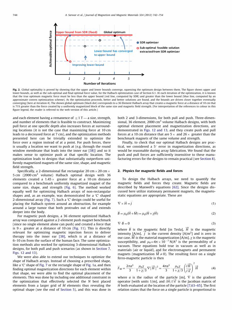
Fig. 2. Global optimality is proved by showing that the upper and lower bounds converge, squeezing the optimum design between them. The figure shows upper and

lower bounds, as well as the sub-optimal and final optimal force value, for the Halbach optimization case of Section 6.1. At each iteration of the optimization, it is known

that the true optimum magnetic force must be less than the upper bound (red line, computed by SDR) and greater than the lower bound (blue line, computed by an

approximate convex optimization scheme). As the optimization proceeds, better and better solutions are found, and the bounds are driven closer together eventually

converging (here at iteration 4). The shown global optimum (black dot) corresponds to a 36 Element Halbach array that creates a magnetic force at a distance of 10 cm that

is 71% greater than the force created by a uniformly magnetized block of the same size and magnetic field strength. (For interpretation of the references to colour in this

figure legend, the reader is referred to the web version of this article.)

A. Sarwar et al. / Journal of Magnetism and Magnetic Materials 324 (2012) 742–754744

and each element having a remanence of r1 T — a size, strength,and number of elements that is feasible to construct. Maximizingpull force at one specific depth also increases forces at surround-ing locations (it is not the case that maximizing force at 10 cmleads to a decreased force at 7 cm), and the optimization methodspresented here can be trivially extended to optimize theforce over a region instead of at a point. For push forces, thereis usually a location we want to push at (e.g. through the roundwindow membrane that leads into the inner ear [38]) and so itmakes sense to optimize push at that specific location. Theoptimization leads to designs that substantially outperform uni-formly magnetized magnets of the same size, shape, and magneticfield strength.

Specifically, a 2-dimensional flat rectangular 20 cm�20 cm�5 cm (2000 cm3 volume) Halbach optimal design with 36elements created a 1.45� greater force at a 10 cm distancecompared to a benchmark uniformly magnetized magnet of thesame size, shape, and strength (Fig. 6). The method workedequally well for optimizing Halbach arrays of non-rectangularshapes and, as an example, was demonstrated for a ‘C’ shaped2-dimensional array (Fig. 7). Such a ‘C’ design could be useful forplacing the Halbach system around an obstruction, for examplearound a large tumor that both protrudes out of and extendsdeeper into the body.

For magnetic push designs, a 36 element optimized Halbacharray was compared against a 2-element push magnet benchmark(since no single element alone can push) and created a force thatis 9� greater at a distance of 10 cm (Fig. 11). This is directlyrelevant for optimizing magnetic injection forces to delivertherapy into the inner ear [38], which is at a distance of6–10 cm from the surface of the human face. The same optimiza-tion methods also worked for optimizing 3-dimensional Halbachdesigns, for both pull and push scenarios (as shown in Section 7,Figs. 12 and 13).

We were also able to extend our techniques to optimize theshape of Halbach arrays. Instead of choosing a prescribed shape,like a ‘C’ shape of Fig. 7 or the rectangle shape of Fig. 1a, and thenfinding optimal magnetization directions for each element withinthat shape, we were able to find the optimal placement of theelements. This was done by including one additional constraint inthe optimization that effectively selected the N best placedelements from a larger grid of M elements thus revealing theoptimal shape (see the end of Section 5), and this was done in

both 2 and 3-dimensions, for both pull and push. Three-dimen-sional, 36 element, 2000 cm3 volume Halbach designs, with bothoptimal element placement and magnetization directions, aredemonstrated in Figs. 12 and 13, and they create push and pullforces at a 10 cm distance that are 5� and 26� greater than thebenchmark magnets of the same volume and strength.

Finally, to check that our optimal Halbach designs are prac-tical, we considered a 51 error in magnetization directions, aswould be reasonable during array fabrication. We found that thepush and pull forces are sufficiently insensitive to these manu-facturing errors for the designs to remain practical (see Section 8).

2. Physics for magnetic fields and forces

To design the Halbach arrays, we need to quantify themagnetic fields and forces they create. Magnetic fields aredescribed by Maxwell’s equations [62]. Since the designs dis-cussed here utilize stationary permanent magnets, the magneto-static equations are appropriate. These are

r � H,¼ j

,ð1Þ

B,¼ m0ðH

,þM

,Þ ¼ m0ðH

,þwH

,Þ ð2Þ

rUB,¼ 0 ð3Þ

where B,

is the magnetic field [in Tesla], H!

is the magneticintensity [A/m], j

!is the current density [A/m2] and is zero in

our case, M!

is the material magnetization [A/m], w is the magneticsusceptibility, and m0¼4p�10�7 N/A2 is the permeability of avacuum. These equations hold true in vacuum as well as inmaterials (air or liquid), and for electromagnets and permanentmagnets (magnetization M

!a0). The resulting force on a single

ferro-magnetic particle is then

F,

M ¼2pa3

3U

m0w1þw=3

r:H!

:2¼

4pa3

3U

m0w1þw=3

@H!

@ x!

!T

H!

ð4Þ

where a is the radius of the particle [m], r is the gradientoperator [with units 1/m], and @H

,=@ x!

is the Jacobian matrix ofH,

both evaluated at the location of the particle [7,63–65]. The firstrelation states that the force on a single particle is proportional to

A. Sarwar et al. / Journal of Magnetism and Magnetic Materials 324 (2012) 742–754 745

its volume and the gradient of the magnetic field intensitysquared — i.e. a ferro-magnetic particle will always experiencea force from low to high applied magnetic field. The secondrelation, which is obtained by applying the chain rule to the firstone, is more common in the magnetic drug delivery literature andshows that a spatially varying magnetic field (@H

,=@x

,a0) is

required to create a magnetic force. Thus, in order to maximizethe force experienced by a given particle, the gradient of themagnetic field squared must be maximized. This is the only termcontrolled by the magnet design; all other terms depend on thesize and material properties of the particles.

3. Problem formulation

Consider a Halbach array composed of permanent rectangularsub-magnets arranged in a rectangular formation, each magne-tized uniformly in a given direction. The optimization task is toselect the magnetization directions to maximize pull or pushforces on particles located at a specific distance from the magnet.Fig. 3 shows a schematic of a 2-dimensional Halbach arraysample. As illustrated, the goal is to choose the optimal magne-tization directions (indicated by the blue arrows) to maximize thepull or push magnetic force at (x0,y0). Deep reach can beoptimized by maximizing the pull or push forces at a (x0,y0)location far from the Halbach array.

If the strength of the Halbach array is unrestricted, then themagnetic force can be increased simply by making the magnetsstronger. However, there are practical constraints on the availablestrengths of permanent magnets as well as regulatory safetyconstraints on the strength of the magnetic field that can beapplied across the human body (the United States Food and DrugAdministration currently considers 8 T fields safe for adults andup to 4 T appropriate for children [66]). Thus the desired optimi-zation problem is to maximize the magnetic force given amaximum allowable magnetic field strength. For convenience,and since permanent NdFeB magnets can be purchased withremanence magnetization of around 1 Tesla, we limit the magne-tization of each Halbach element to 1 T.

The magnetic field around a uniformly magnetized rectangularmagnet is known analytically. Here the analytical expressiondeveloped by Herbert and Hesjedal [67] is used to express themagnetic field around a Halbach array with sub-magnets havingarbitrary magnetization directions. The magnetic field from twoor more magnets can be added together to establish the netmagnetic field. This is a standard assumption in the design ofHalbach arrays [31], and it is true as long as the magnetic fieldarising from the combination of sub-magnets does not causepartial or complete demagnetization or magnetization reversals[68]. The designs we present in this paper do not generatedemagnetizing fields strong enough to cause partial or completedemagnetization of the sub-magnets involved.

Fig. 3. Schematic of Halbach array of N magnets arranged in rectangle formation. Each

directions. The goal is to find the angle y for each sub-magnet in order to maximize th

colour in this figure legend, the reader is referred to the web version of this article.)

Let A!ðx,yÞ represent the analytical expression for the magnetic

field around a rectangular magnet that is uniformly magnetized

along the positive horizontal axis, and let B!ðx,yÞ represent the

analytical expression for the same magnet uniformly magnetizedalong the positive vertical axis. Then the magnetic field when this

magnet is uniformly magnetized at an angle y is given by

A!ðx,yÞcosyþ B

!ðx,yÞsiny. The magnetic field around the entire

Halbach array is generated by translating and adding togethersolutions for all the elements. For the ith Halbach element atlocation (ai,bi), with (as yet unspecified) magnetization direction

yi, let ai¼cos yi and bi¼sin yi. The magnetic field created atlocation (x0,y0) by this element is

H!

iðx0,y0Þ ¼ ai A!ðx0�ai,y0�biÞþbi B

!ðx0�ai,y0�biÞ ð5Þ

The coefficients ai and bi are the unknown design variables. Inorder to limit the strength of any given element to 1 Tesla, theconstraint ai

2þbi

2r1 is imposed for all i. For a Halbach arraycontaining N sub-magnets, the expression for the magnetic fieldat point (x0,y0) is

H!ðx0,y0Þ ¼

XN

i ¼ 1

ai A!ðx0�ai,y0�biÞþbi B

!ðx0�ai,y0�biÞ ð6Þ

The relationship between the design variables ai and bi and themagnetic force exerted by the Halbach array at point (x0,y0) isquadratic in the variables ai and bi. According to Eq. (4), thestrength of the magnetic force experienced by a magnetic particleat a point (x0,y0) is directly proportional to the gradient of thesquare of the magnetic field at that point. Define

A!

i : ¼ A!ðx0�ai,y0�biÞ ð7Þ

and

B!

i : ¼ B!ðx0�ai,y0�biÞ ð8Þ

Squaring Eq. (6) and taking the gradient, the expression forrH!2

ðx0,y0Þ becomes

rH!2

ðx0,y0Þ

¼rXN

j ¼ 1

XN

i ¼ 1

ðaiaj A!

iU A!

jþaibj A!

iU B!

jþbiaj B!

iU A!

jþbibj B!

iU B!

jÞ

0@

1Að9Þ

The gradient operator r is linear. Since the coefficients ai andbi are not functions of x and y they can be pulled out of thesummation. The resulting Eq. (10) shows how the magnetic forceof Eq. (4) depends on the Halbach array design variables ai and bi:

rH!2

ðx0,y0Þ ¼XN

j ¼ 1

XN

i ¼ 1

ðaiajrð A!

iU A!

jÞþaibjrð A!

iU B!

jÞ

þbiajrð B!

iU A!

jÞþbibjrð B!

iU B!

jÞÞ ð10Þ

green box represents a sub-magnet. The blue arrows show possible magnetization

e push or pull force at the location (x0,y0). (For interpretation of the references to

A. Sarwar et al. / Journal of Magnetism and Magnetic Materials 324 (2012) 742–754746

The Halbach array optimization problem can now be stated inmatrix form. The goal is to maximize magnetic pull or push forcesalong the horizontal axis and, thus, the focus is solely on the

horizontal component of rH!2

ðx0,y0Þ, i.e. ðrH!2

ðx0,y0ÞÞx : ¼

rH!2

ðx0,y0ÞUð1,0Þ. Define the matrix P as

P : ¼

ðrðA1UA1ÞÞx � � � ðrðA1UANÞÞx ðrðA1UB1ÞÞx � � � ðrðA1UBNÞÞx

^ & ^ ^ & ^

ðrðANUA1ÞÞx � � � ðrðANUANÞÞx ðrðANUB1ÞÞx � � � ðrðANUBNÞÞx

ðrðB1UA1ÞÞx � � � ðrðB1UANÞÞx ðrðB1UB1ÞÞx � � � ðrðB1UBNÞÞx

^ & ^ ^ & ^

ðrðBNUA1ÞÞx � � � ðrðBNUANÞÞx ðrðBNUB1ÞÞx � � � ðrðBNUBNÞÞx

0BBBBBBBBB@

1CCCCCCCCCAð11Þ

and define the vector q!

as a concatenated list of the design

variables ai and bi as

q!T

: ¼ ða1,. . .,aN ,b1,. . .,bNÞT

ð12Þ

Now ðrH!2

ðx0,y0ÞÞx can be written in a compact form as

ðrH!2

ðx0,y0ÞÞx ¼ q!T

P q!

ð13Þ

This equation succinctly states how the horizontal magneticforce strength depends on the Halbach design variables. Toinclude the ai

2þbi

2r1 magnetization constraints, let Gi be a2N�2N matrix having unity at the locations (i,i) and (Nþ i,Nþ i),and with zeros everywhere else. Then the element magnetizationconstraints can be written in matrix form as

q!T

Gi q!r1 ð14Þ

for all i, The force optimization problem can, therefore, be statedas follows: maximize (for push) or minimize (for pull) the

quadratic cost q!T

P q!

of Eq. (13) subject to the N constraints ofEq. (14), one for each Halbach element (for i¼1, 2, y, N).

4. Problem solution

The quadratic optimization problem formulated in the last section(also referred to as a quadratic program) can be solved using variousmethods. It is not convex – the matrix P is not necessarily negative orpositive semi-definite – which implies that it can have many localoptima and hence a globally optimal solution cannot be guaranteed ingeneral. Much of the literature on non-convex quadratic program-ming has focused on obtaining good local minima, using non-linearprogramming techniques [69] such as active-set or interior-pointmethods [70]. Numerous general-purpose optimization techniquescan also be tailored to solve quadratic programs. A review of severaloptimization methods for non-convex quadratic programs can befound in [71,72]. Some machine learning methods – such as thosebased on neural networks [42] – have also been used to solve thisclass of problems. However, for non-convex problems, these methodsoften get stuck in local optima [41,43].

We employ a combination of 2 methods to find the optimalsolutions and determine the upper and lower bounds for theoptimal force: (1) semi-definite relaxation [73] and (2) themajorization method [74]. Rigorous bounds provide informationon the quality of the optimal solution. If, for example, it is knownthat the maximum achievable force is guaranteed to be betweenFL and FU, and the found optimum has a force F in the top range ofthe bracket close to FU, then the found solution is a high qualityoptimum close to the true (global) maximum. If, as in Fig. 2, andas occurs for all the Halbach optimization cases in this paper, thetwo bounds converge, then we additionally know for certain thata global optimum has been achieved.

To find the upper bound for a maximum push (or pull) force,semi-definite relaxation (SDR) [73] is employed. This methodconverts the original non-convex quadratic problem into a closelyrelated convex problem by a change of variables and a constraintrelaxation. Finding a solution to the new SDR problem is mucheasier, is numerically more efficient, and a global optimum to therelaxed, changed-variables problem is guaranteed [73]. The globaloptimum of the relaxed SDR problem is an upper bound for theglobal optimum of the original non-convex quadratic problem(this upper bound is illustrated as the red line in Fig. 2).

To compute the lower bound, re-scaling the above SDR solution tosatisfy the constraints yields a solution, a magnet design, that satisfiesall the constraints but that is sub-optimal (the first open circle atiteration 1 in Fig. 2) — this solution is a lower bound for the globaloptimum of the original non-convex quadratic program (bottom mostdashed gray line). The scaled sub-optimal solution can then beimproved by optimizing a convex function that approximates theoriginal non-convex cost function. The solution to this approximateconstrained convex problem leads to an improved sub-optimalsolution (second open circle in Fig. 2) and provides a tighter lowerbound (higher dashed gray line). The next iteration yields a third sub-optimal solution and a better third lower bound. The process repeatsuntil no further improvement is possible or until the lower boundreaches the upper bound proving that a global optimum of theoriginal problem has been found.

Below we first discuss the mathematical details of the relaxed–constraint convex SDR process and the upper bound that it yields.Then we describe the iteration of approximate convex problems thatgives a succession of sub-optimal solutions and improved lowerbounds. When these lower bounds converge to the upper bound thelast solution is guaranteed to be the global optimum Halbach design.

The mathematics is presented for optimizing push. Maximizingpull proceeds in exactly the same way except that the cost function

q!T

P q!

is replaced by its negative� q!T

P q!

and this oppositely signedfunction is then minimized. The conversion from the original non-convex problem to a convex matrix problem is achieved by a changeof variables. The SDR corresponding to the original optimizationproblem of Eqs. (13) and (14) can be re-stated as follows. The P andGi matrices are symmetric. For symmetric matrices

q!T

P q!¼ Trð q

!TP q!Þ¼ TrðP q

!q!TÞ ð15Þ

q!T

Gi q!¼ Trð q

!TGi q!Þ¼ TrðGi q

!q!TÞ ð16Þ

where the trace operator Tr( � ) is the sum of the elements on themain diagonal of a square matrix. Define the new matrix variable

Q : ¼ q!

q!T

as the outer product of the q!

vector with itself. Thisrecasts the cost and constraints into linear functions of Q

q!T

P q!¼ TrðPQ Þ ð17Þ

q!T

Gi q!¼ TrðGiQ Þ ð18Þ

however, not all Q’s are permissible. Only Q matrices that can be

formed by the outer product of a single vector, i.e. of the form Q :

¼ q!

q!T

should be considered, and this is the set of matrices that arepositive semidefinite (QZ0) with unit rank [75]. Thus the optimiza-tion can be rephrased as maximize or minimize Tr(PQ) subject to theNþ2 constraints: Tr(GiQ)r1 for i¼1,2, y N; QZ0; and rank(Q)¼1.The cost and the first Nþ1 constraints are convex in Q [45]. However,the last rank constraint is not convex. If this rank constraint isremoved then the problem becomes convex and a global optimumcan be readily found. Removing the rank constraint allows a wider

choice of Q solutions: it includes the Q : ¼ q!

q!T

case but also allowsother solutions that are not the outer product of a single vector. Thus

A. Sarwar et al. / Journal of Magnetism and Magnetic Materials 324 (2012) 742–754 747

the cost attained by solving this new convex problem is guaranteed tomatch or exceed the cost that can be achieved for the original non-convex constrained quadratic problem – if Q* is the global optimalsolution to the relaxed convex problem with achieved cost Tr(PQ*),

and q!n

is the (still unknown) global solution to the original quadraticproblem of Eqs (13) and (14), then it is guaranteed that

q!nT

P q!n

rTrðPQnÞ. Thus TrðPQn

Þ is an upper bound to the trueglobal optimum (it is the red line in Fig. 2).

The optimal solution Q* of the relaxed convex problem alsoprovides a lower bound to the true global optimum after an

appropriate rescaling. Let v!n

be the eigenvector of Q* that has the

maximum eigenvalue. In order for v!n

to qualify as a sub-optimalfeasible solution to the original non-convex quadratic problem, it

must satisfy the N constraints v!nT

Gi v!n

r1 for all i¼1, 2, y, N. Let t

be the maximum value that the expression v!nT

Gi v!n

achieves for all

i, so define t : ¼maxið v!nT

Gi v!n

Þ. By definition v!nT

Gi v!n

rt for all i.

Now let q!

# : ¼ v!n

=ffiffiffitp

then q!

#

TGi q!

# : ¼ ð v!nT

=ffiffiffitpÞGið v!n

=ffiffiffitpÞ

r1 so that this new scaled vector q,

# satisfies the N constraints

q!

#

TGi q!

#r1 for all i¼1, 2, y, N. It is therefore a feasible sub-optimal solution to the original non-convex quadratic program. Asub-optimal solution cannot beat the maximum possible pull or pushforce and is therefore a guaranteed lower bound to the original

problem, i.e. q!nT

P q!n

Z q!

#

TP q!

#. This first lower bound is shownby the lowest dashed gray line in Fig. 2.

The task now is to improve the lower bound. Any vector q!

thatsatisfies the constraints of the original problem yields at least a sub-optimal solution, and hence provides a lower bound to the optimalmagnetic force. In order to further improve the lower bound achievedby q

,

#, the original quadratic problem is approximated with a convexfunction without relaxing any constraints. This convex function isformulated in such a way that optimizing it also produces an optimal(but possibly local) solution to the original quadratic problem.

To define this new convex function, we proceed as follows.

Note that maximizing q!T

P q!

is equivalent to minimizing

f ð q!Þ : ¼� q

!TP q!

. Define the new function Fð q!Þ, which is called

the convex quadratic majorizer [74] of f ð q!Þ at q

,

#, as

Fð q!Þ : ¼ f ð q

!#Þþð q!� q!

#ÞTrf ð q!Þ9

q!

#

þlð q!� q!

#ÞTð q!� q!

#Þ ð19Þ

where r denotes the gradient operator with respect to q,

,

rf ð q!Þ9

q!

#

is the gradient of f ð q!Þ with respect to q

,and then

Fig. 4. Design of Halbach array with optimal shape and magnetization. Step 1: conside

then find the N most significant sub-magnets that maximize the force (push or pull) at

that the force (push or pull) is maximized at (x0,y0).

evaluated at q,

#, l¼max½0,lmaxðPÞ�, and lmax(P) denotes themaximum eigenvalue of the matrix P. That the function F is a

convex quadratic majorizer of f at q,

# means that f ð q!ÞrFð q

!Þ for

all q,

, and f ð q!Þ¼Fð q!Þ for q

,¼ q

,

# [74]. If q,

## minimizes F, then we

have the sandwich inequality f ð q!

##ÞrFð q!

##ÞrFð q!

#Þ ¼ f ð q!

#Þ.The first inequality shows that minimizing F implies decreasing

the value of the objective function f ð q!Þ, which is equivalent to

increasing the value of q!T

P q!

.

Unlike f, the function F is convex in q,

because f ð q!

#Þ is a

constant offset, ð q!� q!

#ÞTrf ð q!Þ9

q!

#

is linear in q,

, and

lð q!� q!

#ÞTð q!� q!

#Þ is purely quadratic with lZ0. Thus the

new approximate problem: minimize Fð q!Þ subject to the same

constraints as the original problem q!T

Gi q!r1 for i¼1, 2, y, N, is

convex and its global optimum q!

## can be found. Since F is only

an approximation to the true cost f ¼� q!T

P q!

, its global opti-mum is a feasible but sub-optimal solution of the original non-convex problem. As such, it provides the next lower bound

q!nT

P q!n

Zq,T

##Pq,

##. This second lower bound is shown as the

second dashed blue line in Fig. 2. At the next iteration, q!

# is

replaced by q!

## in F of Eq. (19), a new sub-optimal solution q!

###

is found, and the process repeats until the lower bound cannot beimproved any further. In Fig. 2 this occurs at the 4th iteration, and

the final Halbach array design vector q,n

¼ q!

#### has a lower

bound that achieves the upper bound proving that q,n

¼ q!

#### is aglobal optimum of the original non-convex constrained optimiza-tion problem — it is the best possible solution of the Halbachdesign problem posed in Fig. 3 and Eqs. (13) and (14).

In addition to optimizing magnetization directions for a fixedHalbach array shape (as in Fig. 3 for a rectangular array), it is alsopossible to use the same methods to choose optimal array shapes.The additional key idea is simple and is shown in Fig. 4. Suppose wewant to design an optimal Halbach array, in shape and magnetizationdirections, using only N magnets. A grid of M magnets is consideredwhere M4N and an optimization is used to determine the sub-set ofN magnets that are most significant—this determines the shape of thearray (step 1 in the figure). The second step is to then re-compute theoptimal magnetization directions for this shape. Together, this finds amagnet design that has both the best shape and the best magnetiza-tion directions for a specified magnet volume (equivalently for arestricted number of magnet elements).

r M sub-magnets arranged in a rectangular shape larger than the desired magnet,

(x0,y0). Step 2: Given these N sub-magnets, find their respective magnetization so

A. Sarwar et al. / Journal of Magnetism and Magnetic Materials 324 (2012) 742–754748

Mathematical formulation of Step 1, to select the best N out ofM elements, is very similar to what has already been done. Thenew part is to effectively restrict the number of elements to justN, and this can be done by adding a single new constraint. Asbefore, we maximize (for push) or minimize (for pull) the

quadratic cost q!T

P q!

, as shown in Eq. (13), but now for M

(4N) sub-magnets. Hence we state M constraints q!T

Gi q!r1

(for i¼1,2,y, M) as we still want to limit the strength of eachelement to 1 T. One additional constraint effectively restricts thenumber of magnets back to only N by requiring the sum of the

squares of all the design variables ai and bi to be less than N, i.e.,PMi ¼ 1 a2

i þb2i rN. Dividing by N, this new constraint can be

written in the matrix form (remember that the vector q!

now

Fig. 5. Benchmark magnet. Schematic showing the axis system and chosen

optimization location for a benchmark uniformly magnetized rectangular magnet

with height h¼20 cm, width w¼20 cm, and thickness t¼5 cm. The optimization

point is located at x¼10 cm, y¼h/2 cm, and z¼t/2 cm. This magnet is used as a

benchmark for both the 2D and 3D pull design cases.

-0.25 -0.2 -0.15 -0.1 -0.05

-0.15

-0.10

-0.05

0

0.05

0.10

0.15

Magnetic Field Exponent (Log||H||, cont(small maroon arrows) [

x [m]c=Fx(opt pull)/ Fx(unif

y [m

]

Fig. 6. Optimal 36 element 2D pull array. The black dot identifies the optimization poin

indicates the logarithm of the magnetic field strength at that location (for example,

dimensionless factor ‘c’ is the ratio of the pull force for this 36 element optimal Halbach

has a height, width, and thickness of h¼3.33 cm, w¼3.33 cm, and t¼5 cm. The magne

gradient to the optimization point to create a maximum force. (For interpretation of the

of this article.)

has a length of 2M) as

q!T 1

NG

� �q!r1 ð20Þ

where G is the identity matrix of size 2M. When this optimizationis solved as before, we select the N sub-magnets with the greatestvalues of ai

2þbi

2 to conclude step 1. Then step 2 proceeds exactlyas before except now the rectangular arrangement of elements inFig. 3 is replaced by the new arrangement of array elementsdetermined in step 1. The end result is both an optimal arrayshape and element magnetization directions.

5. Optimized 2D Halbach array designs

In this section we begin to show the results of the optimizationmethods. We start with arrays of a fixed shape (no shapeoptimization yet) and present various designs of optimized2-dimensional Halbach arrays for maximum pull and push forceobjectives. In line with the problem formulated in Section 4, it isassumed that the array elements can only be magnetized in the xy

plane. Magnetization along the z-axis is set to zero. In all of thedesigns presented, the force is optimized at a distance of 10 cmfrom the edge of the array. This allows for meaningful compar-isons to be made. Various designs to achieve maximum pull forcesare discussed first.

5.1. Maximum pull force designs

Maximizing the pull force translates to minimizing the hor-izontal force, making it as negative as possible. Since the goal is tosee if the optimized Halbach arrays can perform better than asimple uniformly magnetized magnet, for example as used in[47], all designs are benchmarked against such a rectangular

0 0.05 0.1 0.15

ours) and Direction VectorsH units A/m]

orm pull)=1.45

7.98.18.38.58.79.09.39.69.910.210.410.711.011.311.611.912.212.412.713.013.3

t and the black arrow shows the direction of the pull force at that point. The color

a light to medium orange contour of 10.2 corresponds to :H:¼1010.2 A/m). The

array to the pull force from the benchmark uniform magnet of Fig. 5. Each element

tizations of the array ‘‘fan in’’ as this formation focuses the magnetic field and its

references to colour in this figure legend, the reader is referred to the web version

A. Sarwar et al. / Journal of Magnetism and Magnetic Materials 324 (2012) 742–754 749

magnet of the same size and 1 T magnet strength. Considering abenchmark magnet of 20 cm height, 20 cm width, and 5 cmthickness, the reference point (the desired point for optimizingthe force in a Halbach array of the same dimensions) is chosen ata horizontal distance of 10 cm from the vertical right edge of themagnet (as shown in Fig. 5).

Recall that the magnetic force (pull or push) is proportional tothe horizontal component of the gradient of the magnetic fieldsquared: ðrH

!2

ðx0,y0ÞÞx. The benchmark rectangular magnet hasðrH!2

ðx0,y0ÞÞx¼–4.39�1010 A2/m3, with the negative sign indi-cating a pull force.

Fig. 6 illustrates the optimal magnetization directions for aplanar 36 element Halbach array with the same overall shape(rectangle) and volume as the benchmark magnet of Fig. 5. Theforce was optimized at a point 10 cm away from the right mostface of the array. The pull force generated by this optimal2-dimensional Halbach design is 1.45� more than that generatedby the benchmark uniform magnet of the same strength andvolume. The optimization to determine this design took 4 min torun on a computer with an Intels CoreTM i7 processor with 8 GBRAM using MATLAB version 7.9.0.

Next we show that the optimization method works equallywell for other pre-determined shapes besides a rectangle. As anexample, we consider a ‘C’ shape with the same volume as thebenchmark magnet shown in Fig. 5 and again optimize with 36-elements (again of identical size) the pulling force at a distance of10 cm. Such a ‘C’ shape could be appropriate for placing a Halbacharray around a protrusion from the body such as a large tumorthat extends out of as well as into the body. The optimal ‘C’ arrayshown in Fig. 7 generates a pull force that is 2.16� more thanthat generated by the uniformly magnetized benchmark magnet,and it enables a 49% improvement in force over the optimalrectangular array of Fig. 6 demonstrating that array geometry can

-0.2 -0.1 0 0.1

-0.25

-0.20

-0.15

-0.10

-0.05

0

0.05

0.10

0.15

0.20

0.25

Magnetic Field Exponent (Log||H||, contours) and Direction Vectors (small maroon arrows) [H units A/m]

x [m]c=Fx(opt pull)/ Fx(uniform pull)=2.16

y [m

]

7.37.68.08.48.89.19.59.910.210.611.011.411.712.112.512.913.213.6

Fig. 7. Optimal magnetization directions for a ‘C’-shaped 36 element Halbach

array. The coloring scheme here is the same as in Fig. 6. The magnetizations of the

block on the left fan in to concentrate the magnetic field and its gradient at the

optimization point, whereas the blocks on the top and bottom provide a flux

return and add to the horizontal component of the force. (For interpretation of the

references to colour in this figure legend, the reader is referred to the web version

of this article.)

play a significant role in improving magnetic forces. This case alsotook 4 min to run on the same computer (Intels CoreTM i7processor, 8 GB RAM using MATLAB version 7.9.0).

Fig. 8 illustrates both the optimal shape and magnetizationdirections for a planar 36 element Halbach array with the samevolume as the benchmark magnet of Fig. 5. To find the optimalplacement of the 36 elements, a grid of M¼18�18¼324elements was considered, and the 36 most significant elementswere chosen by the optimal element selection method describedearlier. The force was optimized at a point 10 cm away from theright most face of the array. The pull force generated by thisoptimal 2-dimensional Halbach design shown in Fig. 8 is 1.71�more than that generated by the benchmark uniform magnet ofthe same strength and volume. This case took 17 min to optimize.

5.2. Maximum push force designs

Although a single magnetic element will always attract nano-particles towards itself, a correct arrangement of just two elementscan push – and thus magnetically inject – particles. Magneticpushing is useful for a variety of clinical applications such asmagnetically injecting therapy into wounds, infections, or inner eardiseases [38]. Pushing works by creating a magnetic cancellationnode at a distance. Magnetic forces then radiate outwards fromthat cancellation causing a push force on the far side of the node(see [38] for details). As for pull applications, there is a need tooptimize magnet arrangements to reach deeper, push harder, andto do so with shaped arrays that can be fit around obstructions orminimized in size so that they can be inserted into confined spaces.

Maximizing push is equivalent to maximizing the cost func-tion of Eq. (13). (For pull we minimized this function.) It is notpossible to benchmark pushing against a single uniformly mag-netized magnet, since such a single element will always pullparticles towards itself. Instead the push designs are bench-marked against a minimal Halbach array consisting of just tworectangular magnets, one on top of the other (see Fig. 9), with aremanence of 1 T each. The overall dimensions of the array are thesame as that of the benchmark pull magnet shown in Fig. 5(w¼20 cm, h¼20 cm, and t¼5 cm). For this 2-element push

benchmark we have ðrH!2

ðx0,y0ÞÞx¼þ2.94�108 A2/m3 at a dis-tance of 10 cm with the positive sign indicating the push force.

Fig. 10 illustrates the optimal magnetization directions for a planar36 element Halbach array with the same overall shape (rectangle)and volume as the benchmark push array of Fig. 9. The force wasoptimized at a location 10 cm away from the right most face of thearray. The push force generated by this optimal 2-dimensionalHalbach design shown in Fig. 10 is 4.81� more than that generatedby the benchmark push array of same magnetic field strength andvolume. This case took 4 min to run on the computer as before.

Next we show optimization of both element placing andmagnetization directions for maximal pushing at a 10 cm dis-tance. We consider a 36 element array of the same strength andvolume as the push benchmark magnet of Fig. 9. To find theoptimal shape, the optimization selected N¼36 most significantelements from a grid of M¼18�18¼324 elements. The optimalarray is shown in Fig. 11 and generates a push force that is morethan nine times that of the benchmark array of the same strengthand volume. This case took 17 min to evaluate.

6. Optimized 3D Halbach arrays

The previous optimization results were stated in 2 spatial dimen-sions only. We now consider optimizing 3 dimensional arrays. Themathematics remains the same: the problem statement of Section 4

-0.25 -0.2 -0.15 -0.1 -0.05 0 0.05 0.1 0.15

-0.15

-0.1

-0.05

0

0.05

0.1

0.15

Magnetic Field Exponent (Log||H||, contours) and Direction Vectors (small maroon arrows) [H units A/m]

x [m](∇ H2)x=2.94 × 108 A2/m2

y [m

]

5.76.16.67.07.57.88.48.89.39.710.210.611.111.512.012.412.913.3

cancellation node

Fig. 9. The push benchmark magnet. Since a single element cannot push, we use a minimal 2-element design as the benchmark with the magnetization directions

optimally chosen to create a push at a 10 cm distance. The coloring scheme here is the same as in Fig. 6. (For interpretation of the references to colour in this figure legend,

the reader is referred to the web version of this article.)

-0.2 -0.1 0 0.1

-0.2

-0.15

-0.1

-0.05

0

0.05

0.1

0.15

0.2

Magnetic Field Exponent (Log||H||, contours) and Direction Vectors(small maroon arrows) [H units A/m]

x [m]c=Fx(opt pull)/ Fx(uniform pull)=1.71

y [m

]

8.28.58.99.29.59.810.110.410.711.011.311.611.912.212.512.813.113.4

Fig. 8. Plot showing the optimal arrangement and magnetization directions (indicated using large maroon arrows) for a 36 element Halbach array with the same volume

as the benchmark magnet. The coloring scheme here is the same as in Fig. 6. Intuitively, the shape optimization has elected to keep those elements that are closest to the

black optimization point creating a ‘‘pyramid’’ shape. As seen before, the magnetization directions fan in to concentrate the magnetic field and its gradient at the

optimization point. This 2D optimal shape and magnetization array increases the pull force by 71% compared to the benchmark magnet. (For interpretation of the

references to colour in this figure legend, the reader is referred to the web version of this article.)

A. Sarwar et al. / Journal of Magnetism and Magnetic Materials 324 (2012) 742–754750

-0.2 -0.15 -0.1 -0.05 0 0.05 0.1-0.25 0.15

-0.15

-0.10

-0.05

0

0.05

0.10

0.15

Magnetic Field Exponent (Log||H||, contours) and Direction Vectors(small maroon arrows) [H units A/m]

x [m]d=Fx(opt. push)/ Fx(1x2 opt.push)=4.82

y [m

]

5.45.86.16.36.77.27.68.18.58.99.49.810.310.711.211.612.112.513.013.413.9

cancellation node

Fig. 10. Optimal magnetization for a 36 element Halbach push array with the same volume as the benchmark array of Fig. 9. Each element has dimensions of h¼3.33 cm,

w¼3.33 cm, and t¼5 cm. The factor ‘d’ is the ratio of the push force for this optimal array versus the benchmark 2-element array. The coloring scheme is the same as used

in Fig. 6. The elements closer to the optimization point orient to induce a cancellation node, while the rest align to extend magnetic field and its gradient beyond the

cancellation node to generate a maximal push force.

-0.2 -0.1 0 0.1 0.2

-0.23

-0.15

-0.08

0

0.08

0.15

0.23

x [m]

d=Fx(opt. push)/ Fx(1×2 opt.push)=9.19

y [m

]

Magnetic Field Exponent (Log||H||, contours) andDirection Vectors (small maroon arrows) [H units A/m]

6.56.97.37.78.18.58.99.39.710.110.510.911.311.712.112.613.013.4

cancellation node

Fig. 11. Optimal shape and magnetization for a 36 element push Halbach array

with the same volume as the benchmark array of Fig. 9. Here the shape

optimization has selected elements closest to the optimization point but in two

separate halves. The 8 most-central elements orient to induce a cancellation node,

while the rest fan-in to focus the magnetic field and its gradient beyond the

cancellation node in order to generate the strongest push force. The factor ‘d’ is the

ratio of the push force for this optimal array versus the benchmark 2-element

array. The coloring scheme is the same as used in Fig. 6. (For interpretation of the

references to colour in this figure legend, the reader is referred to the web version

of this article.)

A. Sarwar et al. / Journal of Magnetism and Magnetic Materials 324 (2012) 742–754 751

readily generalizes to the 3rd dimension, and is still solved asdescribed in Section 5. Geometry can now be optimized in threedimensions, and each sub-magnet element can be magnetized by avector that has components in all three directions. As before, in all ofthe 3-dimensional designs the force is optimized at a distance of10 cm from the face of the array to allow for meaningful comparisonwith the associated 2-dimensional cases.

6.1. Maximum pull force design

A pull force optimization is carried out for a 36 element (eachelement a cube) 3 dimensional Halbach array having the sameoverall volume as that of the benchmark magnet of Fig. 5. To findthe optimal shape, the optimization selected the N¼36 mostsignificant elements from a grid of M¼3�10�10¼300 ele-ments. As the elements farther away from the optimizationlocation are less significant, only 3 layers were picked along thehorizontal axis for the grid. The optimal array shape is shown inFig. 12. The force generated by this design at the optimizationpoint is about 5 times greater than that generated by the bench-mark magnet shown in Fig. 5. The added degrees of freedom alongthe z-axis, therefore, provide significant improvement in thedesign of Halbach arrays for pull force applications. This casetook 1 h and 43 min to run on the same computer as previously(Intels CoreTM i7 processor, 8 GB of RAM, using MATLAB version7.9.0).

6.2. Maximum push force design

Comparable to the 3-dimensional pull force design describedabove, a push force optimization is also carried out for a 36 element(each element a cube) 3-dimensional Halbach array of the samestrength and volume as the push benchmark magnet of Fig. 9. To findthe optimal shape, the optimization selected the N¼36 most

Fig. 12. Plot showing the optimal geometry and magnetization directions for a 36

element 3D Halbach pull array (with the same volume as the benchmark pull

magnet shown in Fig. 5). Each element is a cube with every side measuring

3.816 cm. The two layers of the Halbach array along the x-axis (front layer shown

in green, rear in red) are shown apart to better visualize the magnetization

directions. The overall formation of the array is shown at the top right where the

two layers are right next to each other and the optimization point and resulting

force are shown by the black dot and arrow. The 2-layer ‘‘pyramid’’ shape is again

optimal because the most effective elements are the ones closest to the optimiza-

tion point. Also, as before, the magnetization directions ‘‘fan in’’, like in Fig. 8, to

push out and focus the magnetic field to better include the optimization point.

(For interpretation of the references to colour in this figure legend, the reader is

referred to the web version of this article.)

Fig. 13. Plot showing the geometry and magnetization directions for a 36 element

3D Halbach array push design (having the same overall volume as that of the

benchmark Halbach array of Fig. 9). Each sub-magnet is a cube with every side

measuring 3.816 cm. The optimization point and resulting force are shown by the

black dot and arrow. The elements closest to the optimization point orient to

induce a cancellation node like in Fig. 11, while the rest focus to extend the

magnetic field and its gradient beyond the cancellation node in order to generate a

strong push force.

A. Sarwar et al. / Journal of Magnetism and Magnetic Materials 324 (2012) 742–754752

significant elements from a grid of M¼3�10�10¼300 elements.The optimal array is shown in Fig. 13. The force generated by thisdesign at the optimization point is about 26 times greater than thatgenerated by the benchmark magnet shown in Fig. 9. As seen for thepull force design, the added degrees of freedom along the z-axis alsoprovide significant improvement in the design of Halbach arrays forpush force applications. This case took 1 h and 43 min to optimize.

7. Sensitivity analysis of push and pull designs

A sensitivity analysis was carried out to determine how errorsin element magnetization angles will affect the array pull andpush forces. This analysis is included to quantify the effect ofinevitable manufacturing imperfections on the performance ofthe arrays. It was found that the pull force designs were robust toperturbations in magnetization angles. For each pull case, 10independent runs were carried out to capture the extent ofvariations in the forces. Randomly generated perturbations ofup to 51 were introduced in the magnetization angles of eachdesign, simulating reasonable tolerances and variations in themanufacturing of Halbach arrays. The resultant pull forces onlyshowed a variation of 0.3% in magnitude, with a maximum pullforce angle deviation of 0.51 away from the horizontal. Thisindicates that the pull designs are quite robust to reasonablemagnetization manufacturing errors.

Push force design is more sensitive to magnetization angle errors.In a series similar to the one above, 10 independent runs were carriedout for each push force design in order to quantify the variations inpush forces. Randomly generated perturbations of up to 51 wereintroduced in the magnetization angles of each design. The resultantpush forces strayed away from the horizontal by up to 41 on average,and 81 in the most extreme cases. However, the magnitude of forcesalong the horizontal axis exhibited a maximum decrease of only 0.8%.In contrast, the magnitude of forces along the vertical axis (thesewere originally zero) rose significantly — to 13.2% of the nominalmagnitude of the horizontal component of the push forces. This wasexpected since push relies on a magnetic field cancellation and thatcancellation was anticipated to be more sensitive to magnetizationdirection errors, and it implies that more care must be taken in themanufacturing and arrangement of magnets for push force applica-tions than for pull cases.

8. Conclusion

Methods based on semi-definite quadratic programming havebeen presented to optimize Halbach arrays to maximize push andpull forces on magnetic particles at depth. These methods providerigorous upper and lower bounds on optimality and for all the arrayshapes tested; these bounds converged proving that the foundmagnetization directions were globally optimal solutions. The opti-mizations ran in minutes for 2-dimensional arrays, and in less than2 h for 3D arrays, on a desktop PC using MATLAB. They wereappropriate to maximize either pull or push forces at depth for anyprescribed array shapes. An additional constraint and selection of N

out of M most significant elements further allowed the determinationof the optimal shapes of Halbach arrays, in addition to their optimalmagnetization directions. The presented case study designs should befeasible to construct (they are in line with previously constructed 36element 1 T arrays), and were sufficiently insensitive to magnetiza-tion direction errors even for the more sensitive push cases to remainpractical under anticipated manufacturing errors. These designssubstantially outperformed benchmark magnets of the same sizeand magnetic field strength with magnetic push and 3D designsshowing the most benefits. Since depth of treatment is one of the keylimitations for magnetic drug targeting, the presented capabilitiesshould provide a path towards the construction of safe and practicalHalbach arrays to reach deeper tissue targets and thus enablemagnetic treatment of a wider set of patients.

References

[1] A.S. Lubbe, C. Alexiou, C. Bergemann, Clinical applications of magnetic drugtargeting, Journal of Surgical Research 95 (2) (2001) 200–206.

A. Sarwar et al. / Journal of Magnetism and Magnetic Materials 324 (2012) 742–754 753

[2] S.K. Pulfer, S.L. Ciccotto, J.M. Gallo, Distribution of small magnetic particles inbrain tumor-bearing rats, Journal of Neuro-Oncology 41 (2) (1999) 99–105.

[3] R. Jurgons, C. Seliger, A. Hilpert, L. Trahms, S. Odenbach, C. Alexiou, Drugloaded magnetic nanoparticles for cancer therapy, Journal of Physics: Con-densed Matter 18 (38) (2006) S2893–S2902.

[4] E.N. Taylor, T.J. Webster, Multifunctional magnetic nanoparticles for ortho-pedic and biofilm infections, International Journal of Nanotechnology 8 (1/2)(2011) 21–35.

[5] M. Kempe, et al., The use of magnetite nanoparticles for implant-assistedmagnetic drug targeting in thrombolytic therapy, Biomaterials 31 (36) (2010)9499–9510.

[6] R. Bawa, Nanoparticle-based therapeutics in humans: a survey, Nanotechnol-ogy Law and Business 5 (2008) 135.

[7] Z.G. Forbes, B.B. Yellen, K.A. Barbee, G. Friedman, An approach to targeteddrug delivery based on uniform magnetic fields, IEEE Transactions onMagnetics 39 (5) (2003) 3372–3377.

[8] A.S. Lubbe, et al., Preclinical experiences with magnetic drug targeting:tolerance and efficacy, Cancer Research 56 (20) (1996) 4694–4701.

[9] A.S. Lubbe, et al., Clinical experiences with magnetic drug targeting: a phase Istudy with 40-epidoxorubicin in 14 patients with advanced solid tumors,Cancer Research 56 (20) (1996) 4686–4693.

[10] E. Ruuge, A. Rusetski, Magnetic fluids as drug carriers: targeted transport ofdrugs by a magnetic field, Journal of Magnetism and Magnetic Materials 122(1–3) (1993) 335–339.

[11] A. Lubbe, Physiological aspects in magnetic drug-targeting, Journal ofMagnetism and Magnetic Materials 194 (1–3) (1999) 149–155.

[12] C. Alexiou, et al., Magnetic drug targeting—biodistribution of the magneticcarrier and the chemotherapeutic agent mitoxantrone after locoregionalcancer treatment, Journal of Drug Targeting 11 (3) (2003) 139–149.

[13] A.-J. Lemke, M.-I. Senfft von Pilsach, A. Lubbe, C. Bergemann, H. Riess, R. Felix,MRI after magnetic drug targeting in patients with advanced solid malignanttumors, European Radiology 14 (11) (2004) 1949–1955.

[14] C. Alexiou, R. Jurgons, C. Seliger, S. Kolb, B. Heubeck, H. Iro, Distribution ofmitoxantrone after magnetic drug targeting: fluorescence microscopic inves-tigations on VX2 squamous cell carcinoma cells, Zeitschrift fur PhysikalischeChemie 220 (2_2006) (2006) 235–240.

[15] P. Xiong, P. Guo, D. Xiang, J.S. He, Theoretical research of magnetic drugtargeting guided by an outside magnetic field 55 (2006) 4383–4387.

[16] J. Dobson, Gene therapy progress and prospects: magnetic nanoparticle-based gene delivery, Gene Therapy, 13, 4, 283–287, 0000.

[17] J.C. Allen, Complications of chemotherapy in patients with brain and spinalcord tumors, Pediatric Neurosurgery 17 (4) (1991) 218–224 1992.

[18] B. Schuell, et al., Side effects during chemotherapy predict tumour responsein advanced colorectal cancer, British Journal of Cancer 93 (7) (2005)744–748.

[19] V.T. Devita, Cancer: Principles and Practice of Oncology Single Volume, 5thed., Lippincott Williams & Wilkins, 1997.

[20] B. Chertok, et al., Iron oxide nanoparticles as a drug delivery vehicle for MRImonitored magnetic targeting of brain tumors, Biomaterials 29 (4) (2008)487–496.

[21] C. Sun, J.S.H. Lee, M. Zhang, Magnetic nanoparticles in MR imaging and drugdelivery, Advanced Drug Delivery Reviews 60 (11) (2008) 1252–1265.

[22] J. Dobson, Magnetic nanoparticles for drug delivery, Drug DevelopmentResearch 67 (1) (2006) 55–60.

[23] A. Nacev, C. Beni, O. Bruno, B. Shapiro, The behaviors of ferromagnetic nano-particles in and around blood vessels under applied magnetic fields, Journalof Magnetism and Magnetic Materials 323 (6) (2011) 651–668.

[24] A. Nacev, C. Beni, O. Bruno, B. Shapiro, Magnetic nanoparticle transportwithin flowing blood and into surrounding tissue, Nanomedicine (London,England) 5 (9) (2010) 1459–1466.

[25] S. ichi Takeda, F. Mishima, S. Fujimoto, Y. Izumi, S. Nishijima, Developmentof magnetically targeted drug delivery system using superconductingmagnet, Journal of Magnetism and Magnetic Materials 311 (1) (2007)367–371.

[26] O. Rotariu, N.J.C. Strachan, Modelling magnetic carrier particle targeting inthe tumor microvasculature for cancer treatment, Journal of Magnetism andMagnetic Materials 293 (1) (2005) 639–646.

[27] S. Goodwin, C. Peterson, C. Hoh, C. Bittner, Targeting and retention ofmagnetic targeted carriers (MTCs) enhancing intra-arterial chemotherapy,Journal of Magnetism and Magnetic Materials 194 (1999) 132–139.

[28] U.O. Hafeli, K. Gilmour, A. Zhou, S. Lee, M.E. Hayden, Modeling of magneticbandages for drug targeting: button vs. Halbach arrays, Journal of Magnetismand Magnetic Materials 311 (1) (2007) 323–329.

[29] P.A. Voltairas, D.I. Fotiadis, L.K. Michalis, Hydrodynamics of magnetic drugtargeting, Journal of Biomechanics 35 (6) (2002) 813–821.

[30] A.D. Grief, G. Richardson, Mathematical modelling of magnetically targeteddrug delivery, Journal of Magnetism and Magnetic Materials 293 (1) (2005)455–463.

[31] K. Halbach, Design of permanent multipole magnets with oriented rare earthcobalt material, Nuclear Instruments and Methods 169 (1) (1980) 1–10.

[32] D.L. Holligan, G.T. Gillies, J.P. Dailey, Magnetic guidance of ferrofluidicnanoparticles in an in vitro model of intraocular retinal repair, Nanotechnol-ogy 14 (6) (2003) 661–666.

[33] J. Ally, B. Martin, M. Behrad Khamesee, W. Roa, A. Amirfazli, Magnetictargeting of aerosol particles for cancer therapy, Journal of Magnetism andMagnetic Materials 293 (1) (2005) 442–449.

[34] C. Alexiou, R. Jurgons, C. Seliger, O. Brunke, H. Iro, S. Odenbach, Delivery ofsuperparamagnetic nanoparticles for local chemotherapy after intraarterialinfusion and magnetic drug targeting, Anticancer Research 27 (4) (2007)2019–2022.

[35] P. Dames, et al., Targeted delivery of magnetic aerosol droplets to the lung,National Nanotechnology 2 (8) (2007) 495–499.

[36] C. Alexiou, et al., A high field gradient magnet for magnetic drug targeting,IEEE Transactions on Applied Superconductivity 16 (2) (2006) 1527–1530.

[37] A.S..Lubbe, Personal Communication (photograph from one of the patientsfrom the clinical trials of A.S. Lubbe et al. [1996]), May-2007.

[38] B. Shapiro, K. Dormer, I.B. Rutel, A two-magnet system to push therapeuticnanoparticles, AIP Conference Proceedings 1311 (1) (2010) 77–88.

[39] R.D. Kopke, et al., Magnetic nanoparticles: inner ear targeted moleculedelivery and middle ear implant, Audiology and Neurotology 11 (2) (2006)123–133.

[40] R. Cortivo, V. Vindigni, L. Iacobellis, G. Abatangelo, P. Pinton, B. Zavan,Nanoscale particle therapies for wounds and ulcers, Nanomedicine (London,England) 5 (4) (2010) 641–656.

[41] D.P. Bertsekas, D.P. Bertsekas, Nonlinear Programming, 2nd ed., AthenaScientific, 1999.

[42] A. Cichocki, R. Unbehauen, Neural Networks for Optimization and SignalProcessing, 1st ed., Wiley, 1993.

[43] X.-S. Zhang, Neural Networks in Optimization, Springer, 2000.[44] C.A. Floudas, P.M. Pardalos, Encyclopedia of Optimization, 1st ed., Springer,

2001.[45] S. Boyd, L. Vandenberghe, Convex Optimization, Cambridge University Press,

2004.[46] J. Ally, A. Amirfazli, W. Roa, Factors affecting magnetic retention of particles

in the upper airways: an in vitro and ex vivo study, Journal of AerosolMedicine: The Official Journal of the International Society for Aerosols inMedicine 19 (4) (2006) 491–509.

[47] B. Zebli, A.S. Susha, G.B. Sukhorukov, A.L. Rogach, W.J. Parak, Magnetictargeting and cellular uptake of polymer microcapsules simultaneouslyfunctionalized with magnetic and luminescent nanocrystals, Langmuir 21(10) (2005) 4262–4265.

[48] Y. Yang, J.-S. Jiang, B. Du, Z.-F. Gan, M. Qian, P. Zhang, Preparation andproperties of a novel drug delivery system with both magnetic and biomo-lecular targeting, Journal of Materials Science. Materials in Medicine 20 (1)(2009) 301–307.

[49] M. Lohakan, P. Junchaichanakun, S. Boonsang, C. Pintavirooj, A computationalmodel of magnetic drug targeting in blood vessel using finite elementmethod, in: Proceedings of the 2nd IEEE Conference on Industrial Electronicsand Applications, 2007. ICIEA 2007, pp. 231–234.

[50] I. Slabu, A. Roth, T. Schmitz-Rode, M. Baumann, Optimization of magneticdrug targeting by mathematical modeling and simulation of magneticfields, in: J. Sloten, P. Verdonck, M. Nyssen, J. Haueisen (Eds.), 4thEuropean Conference of the International Federation for Medical andBiological Engineering, vol. 22, Springer, Berlin, Heidelberg, 2009,pp. 2309–2312.

[51] M.E. Hayden, U.O. Hafeli, Magnetic bandages’ for targeted delivery oftherapeutic agents, Journal of Physics: Condensed Matter 18 (38) (2006)S2877–S2891.

[52] F.M. Creighton, R.C. Ritter, P. Werp, Focused magnetic navigation usingoptimized magnets for medical therapies, in: Proceedings of the MagneticsConference, 2005. INTERMAG Asia 2005. Digests of the IEEE International,2005, pp. 1253–1254.

[53] F.M. Creighton, Optimal Distribution of Magnetic Material for Catheter andGuidewire Cardiology Therapies, in: Proceedings of the Magnetics Confer-ence, 2006. INTERMAG 2006. IEEE International, 2006, pp. 111–111.

[54] B. Polyak, et al., High field gradient targeting of magnetic nanoparticle-loadedendothelial cells to the surfaces of steel stents, Proceedings of the NationalAcademy of Sciences 105 (2) (2008) 698–703.

[55] B.B. Yellen, Z.G. Forbes, K.A. Barbee, G. Friedman, Model of an approach totargeted drug delivery based on uniform magnetic fields, in: Proceedings ofthe Magnetics Conference, 2003. INTERMAG 2003. IEEE International, 2003,p. EC- 06.

[56] F. Mishima, S. Takeda, Y. Izumi, S. Nishijima, Development of magnetic fieldcontrol for magnetically targeted drug delivery system using a supercon-ducting magnet, IEEE Transactions on Applied Superconductivity 17 (2)(2007) 2303–2306.

[57] S. Fukui, et al., Study on optimization design of superconducting magnet formagnetic force assisted drug delivery system, Physica C: Superconductivity463–465 (2007) 1315–1318.

[58] S. Nishijima, et al., Research and development of magnetic drug deliverysystem using bulk high temperature superconducting magnet, IEEE Transac-tions on Applied Superconductivity 19 (3) (2009) 2257–2260.

[59] J.W. Haverkort, Kenjeres, Optimizing drug delivery using non-uniformmagnetic fields: a numerical study, in: Proceedings of the twenty secondIFMBE, 2009, pp. 2623–2627.

[60] X. Zhang et al., Design, construction and NMR testing of a 1 T Halbach.Permanent magnet for magnetic resonance, presented at the COMSOL UsersConference, Boston, MA, 2005.

[61] J. Zheng, J. Wang, T. Tang, G. Li, H. Cheng, S. Zou, Experimental study onmagnetic drug targeting in treating cholangiocarcinoma based on internalmagnetic fields, The Chinese–German Journal of Clinical Oncology 5 (5)(2006) 336–338.

A. Sarwar et al. / Journal of Magnetism and Magnetic Materials 324 (2012) 742–754754

[62] R.P. Feynman, The Feynman Lectures on Physics (3 Volume Set), AddisonWesley Longman, 1970.

[63] D. Fleisch, A Student’s Guide to Maxwell’s Equations, 1st ed., CambridgeUniversity Press, 2008.

[64] Z.G. Forbes, B.B. Yellen, D.S. Halverson, G. Fridman, K.A. Barbee, G. Friedman,Validation of high gradient magnetic field based drug delivery to magnetiz-able implants under flow, IEEE Transactions on Bio-Medical Engineering 55(2) (2008) 643–649, Pt 1.

[65] B. Shapiro, Towards dynamic control of magnetic fields to focus magneticcarriers to targets deep inside the body, Journal of Magnetism and MagneticMaterials 321 (10) (2009) 1594 1594.

[66] D.W. Chakeres, F. de Vocht, Static magnetic field effects on human subjectsrelated to magnetic resonance imaging systems, Progress in Biophysics andMolecular Biology 87 (2–3) (2005) 255–265.

[67] R. Engel-Herbert, T. Hesjedal, Calculation of the magnetic stray field of auniaxial magnetic domain, Journal of Applied Physics 97 (7) (2005) 074504.

[68] M. Katter, Angular dependence of the demagnetization stability ofsintered Nd–Fe–B magnets, in: Proceedings of the Magnetics Conference,

2005. INTERMAG Asia 2005. Digests of the IEEE International, 2005,pp. 945–946.

[69] S. Burer, D. Vandenbussche, A finite branch-and-bound algorithm for non-convex quadratic programming via semidefinite relaxations, MathematicalProgramming 113 (2) (2006) 259–282.

[70] N.I.M. Gould, P.L. Toint, Numerical Methods for Large-Scale Non-ConvexQuadratic Programming (2001).

[71] P.M. Pardalos, Global optimization algorithms for linearly constrained inde-finite quadratic problems, Computers and Mathematics with Applications 21(6–7) (1991) 87–97.

[72] R. Horst, P.M. Pardalos, Handbook of Global Optimization, 1st ed., Springer,1994.

[73] Zhi-quan Luo, Wing-kin Ma, A.M.-C. So, Yinyu Ye, Shuzhong Zhang, Semi-definite relaxation of quadratic optimization problems, IEEE Signal Proces-sing Magazine 27 (3) (2010) 20–34.

[74] J. de Leeuw, K. Lange, Sharp quadratic majorization in one dimension,Computational Statistics and Data Analysis 53 (7) (2009) 2471–2484.

[75] D.C. Lay, Linear Algebra and its Applications, 4th ed., Addison Wesley, 2011.