optimal fiscal and monetary policy with costly wage bargaining
TRANSCRIPT

Optimal Fiscal and Monetary Policy with
Costly Wage Bargaining∗
David M. Arseneau †
Federal Reserve Board
Sanjay K. Chugh‡
University of Maryland
First Draft: November 2006
This Draft: August 4, 2008
Abstract
Costly nominal wage adjustment has received renewed attention in the design of optimal policy. In
this paper, we embed costly nominal wage adjustment into the modern theory of frictional labor markets
to study optimal fiscal and monetary policy. The main result is that the optimal rate of price inflation is
quite volatile despite the presence of nominal wage rigidities. This finding contrasts with results obtained
in standard sticky-wage models, which employ neoclassical labor markets at their core. In addition, the
tax-smoothing result that lies at the heart of optimal policy prescriptions in standard Ramsey models
does not carry over to a search and bargaining environment. Both results stem from a common source
in our model. Shared rents associated with the formation of long-term employment relationships imply
that the optimal policy entails fluctuations in after-tax real wages much larger than in models with
neoclassical labor markets, in which no such rent-sharing margin exists. The results demonstrate that
the level at which nominal wage rigidity is modeled — whether simply layered on top of a neoclassical
market or articulated in the context of an explicit relationship between workers and firms — can matter
a great deal for policy recommendations.
Keywords: inflation stability, real wage dynamics, Ramsey model, Friedman Rule, labor search
JEL Classification: E24, E50, E62, E63
∗The views expressed here are solely those of the authors and should not be interpreted as reflecting the views of theBoard of Governors of the Federal Reserve System or of any other person associated with the Federal Reserve System. Forhelpful discussions and comments, we especially thank Dale Henderson, seminar and conference participants at the Board’sInternational Finance workshop, the University of Maryland, Georgetown University, the 2007 Econometric Society WinterMeetings (Chicago), and the 2007 SCE Annual Meetings (Montreal), and an anonymous referee and the editor, Robert King,for constructive comments.†E-mail address: [email protected].‡E-mail address: [email protected].
1

1 Introduction
The study of optimal monetary policy in the presence of nominally-rigid wages has enjoyed a resurgence
of late. The typical story behind models featuring nominal wage rigidities is that wage negotiations are
costly or time-consuming, which leads to infrequent adjustments. However, it is somewhat difficult to
understand the idea of wage negotiations, costly or not, when the underlying model of the labor market is
neoclassical, which is true of existing sticky-wage models that study optimal policy. In neoclassical markets,
there are no negotiations — all transactions are simply against the anonymous market. Instead, models that
feature explicit bilateral relationships between firms and workers seem to be called for in order to study the
consequences of costly wage negotiations.
In this paper, we embed costly nominal wage adjustment into the modern theory of frictional labor
markets, which formalizes the notion of long-term employment relationships, to study optimal fiscal and
monetary policy. The main result is that the optimal inflation rate is quite volatile over time despite
the presence of nominal wage rigidities, which stands in contrast to results obtained in environments with
fundamentally neoclassical labor markets. In addition, the typical tax-smoothing incentive at the heart
of optimal policy prescriptions in standard Ramsey models does not carry over into our environment: the
optimal labor tax rate is an order of magnitude more volatile than in a standard Ramsey model. A central
message of our results is thus that the level at which nominal wage rigidity is modeled — whether simply
layered on top of a neoclassical market or articulated in the context of an explicit relationship between
workers and firms — can matter a great deal for policy recommendations.
Since Chari, Christiano, and Kehoe (1991), the cyclical properties of optimal policy in basic Ram-
sey monetary models have been well-understood. One of their main quantitative findings was that, in
an environment with fully-flexible nominal prices and nominal wages, a Ramsey planner engineers large
state-contingent movements in the price level in response to business-cycle magnitude shocks affecting the
consolidated government budget. The Ramsey literature has recently re-examined this issue in models fea-
turing nominally-sluggish prices and wages. Schmitt-Grohe and Uribe (2004a) and Siu (2004) showed that
with even a small degree of nominal rigidity in prices, optimal inflation volatility is quite small. Chugh
(2006) showed that stickiness in nominal wages by itself also makes Ramsey-optimal inflation very stable
2

over time, but in the latter the wage rigidity is introduced in an otherwise neoclassical labor market.
The contrast between the results here and those in Chugh (2006) stems from the importance the planner
attaches to delivering a stable path of aggregate real wages for the economy. The key to understanding the
result in a neoclassical model is that if real wage growth is determined essentially by technological features
of the economy (such as productivity) that do not fluctuate too much, then any desire to stabilize nominal
wages shows up as a concern for stabilizing nominal prices. If real wages are not tied so tightly to an
economy’s production possibilities but instead are free to adjust without much allocative consequence, as
can be the case in an environment with search frictions, then such an effect need not occur. In our model,
wages are determined after a worker and a firm endure a costly search process. Once two parties meet, the
resulting economic rents are divided through wage negotiations. In general, there is a continuum of real
wages that is acceptable for both parties to agree to consummate the match and begin production. In this
sense, the aggregate real wage plays much more of a distributive, rather than a purely allocative, role. Thus,
any desire to stabilize nominal wages does not immediately translate into a desire to stabilize nominal prices.
A similar mechanism underpins the lack of tax-smoothing that is part of the model’s optimal policy
prescription. Werning (2007) and Scott (2007) recently shed new insight on the quantitative finding by
Chari, Christiano, and Kehoe (1991) (henceforth, CCK) that labor tax rates should remain virtually constant
over time in the face of business-cycle shocks. However, this result and intuition rely on neoclassical labor
markets. Because a simple neoclassical relationship between employment and labor taxes does not exist in
a search model, there ought to be no presumption that labor-tax-smoothing should arise in an environment
with fundamental frictions. Indeed, the rent-sharing that makes inflation stability an unimportant goal of
policy is also the driving force behind the unimportance of tax smoothing. Cyclical (and large) variations
in both inflation and tax rates affect the distributional consequences of the real wage through what we refer
to as a dynamic bargaining power effect, but these redistributions have little impact on real allocations.
The primary focus of this study is on the short-run dynamics of optimal policy, but the model also has
predictions for long-run policy. The most notable is that in the long run, the optimal inflation rate trades
off three distortions. Two distortions are standard in monetary models: inefficient money holdings due to a
deviation from the Friedman Rule versus resource losses stemming from nominal adjustment due to non-zero
3
inflation. The third distortion influencing steady-state inflation is inefficiencies in job creation, which positive
inflation in some cases can offset. This latter policy channel is one about which Ramsey models based on
neoclassical labor markets are silent; it is one that others using labor-search frameworks, such as Faia (2008)
and Cooley and Quadrini (2004), have also pointed out, albeit not in the context of a model studying both
fiscal and monetary policy.
Our work is more broadly related to the recent literature exploring the consequence of nominal rigidities
in labor search and matching environments.1 The studies most closely related to ours are Faia (2008) and
Thomas (2008), both of whom study optimal monetary policy in New Keynesian models with labor matching
frictions. In contrast, our model features flexible product prices. Furthermore, rather than concentrating
solely on monetary policy, we conduct a traditional Ramsey exercise in which we solve an optimal public
financing problem that requires specifying fiscal and monetary policy jointly. Despite obvious differences
in implementation, the views emerging from this study and those of Faia (2008) and Thomas (2008) are
complementary.
The rest of the paper is organized as follows. Section 2 builds the basic model. Section 3 presents the
Ramsey problem, and Section 4 presents and discusses the main results. Section 5 summarizes and offers
possible avenues for continued research. In the expanded working paper version, Arseneau and Chugh (2007),
we also allow for an intensive margin of labor adjustment to demonstrate how a more standard neoclassical
hours mechanism affects the results — the impression left by the results in the expanded model is largely
the same as those reported here.
2 Model
As many other recent studies have done, we embed the Pissarides (2000) textbook search model into a
dynamic stochastic general equilibrium framework. We present in turn the composition of the representative
household, the representative firm, a description of wage determination, the actions of the government, and
the definition of a private-sector equilibrium.1For example, Blanchard and Gali (2006, 2007), Walsh (2005), Trigari (2006), Christoffel and Linzert (2005), and Krause
and Lubik (2007), to name just a few.
4
2.1 Households
There is a continuum of measure one of identical households in the economy. The representative household
consists of a continuum of measure one of family members. Each member of the household either works
during a given time period or is unemployed and searching for a job. At time t, a measure nt of household
members are employed and a measure 1 − nt are unemployed. Total household income is divided evenly
amongst all members, so each family member has the same consumption.2
The household’s discounted lifetime utility is given by
E0
∞∑t=0
βt[u(c1t, c2t) +
∫ nt
0
Aihdi+∫ 1
nt
ιidi
], (1)
where u(c1, c2) is each family member’s utility from consumption of cash goods (c1) and credit goods (c2),
h is a fixed number of hours that an employed family member works, Ai is the utility per unit time of an
employed family member i, and ιi is the utility experienced by individual i from non-work. The function
u satisfies uj > 0 and ujj < 0, j = 1, 2. We assume symmetry in the utility amongst all employed family
members, so that Ai = A, as well as symmetry in the utility of non-work amongst all unemployed family
members, so that ιi = ι. Thus, household lifetime utility can be expressed as
E0
∞∑t=0
βt[u(c1t, c2t) + ntAh+ (1− nt)ι
]. (2)
The household does not choose how many family members work; the measure of family members who
work is determined by a labor matching process. Also note, as is common in this class of models, there is no
labor-supply margin. As mentioned above, each employed individual works the fixed number of hours h.3
The household chooses state-contingent sequences of consumption of each good, nominal money holdings,
and nominal bond holdings {c1t, c2t,Mt, Bt}, to maximize lifetime utility subject to an infinite sequence of
2Thus, we follow Merz (1995), Andolfatto (1996), and much of the subsequent literature in this regard by assuming fullconsumption insurance between employed and unemployed individuals.
3The expanded analysis in the working paper examines, among other things, the robustness of the findings here to endogenousadjustment of labor at the hours margin.
5

flow budget constraints
Mt −Mt−1 +Bt +Rt−1Bt−1 = (1− τnt−1)Wt−1nt−1h− Pt−1c1t−1 − Pt−1c2t−1 + Pt−1dt−1 (3)
and cash-in-advance constraints
Ptc1t ≤Mt. (4)
Mt−1 is the nominal money the household brings into period t, Bt−1 is nominal bonds brought into t, Wt is
the nominal wage, Pt is the price level, Rt is the gross nominally risk-free interest rate on government bonds
held between t and t + 1, τnt is the tax rate on labor income, and dt is a flow dividend payment by firms
received lump-sum by households. 4
As is standard in this class of cash/credit models, household optimality yields the Fisher equation
1 = RtEt
[βu1t+1
u1t
1πt+1
](5)
and an optimality condition linking the marginal rate of substitution between cash and credit goods to the
nominal interest rate
u1t
u2t= Rt. (6)
In a monetary equilibrium, Rt ≥ 1, otherwise consumers could earn unbounded profits by buying money
and selling bonds, thus placing an equilibrium restriction on the MRS between cash and credit goods.
2.2 Production
The production side of the economy features a representative firm that must open vacancies, which entail
costs, in order to hire workers and produce. The representative firm is “large” in the sense that it operates
many jobs and consequently has many individual workers attached to it through those jobs.
To be more specific, the firm requires only labor to produce its output. The firm must engage in costly
search for a worker to fill each of its job openings. In each job k that will produce output, the worker and4The timing of the budget and cash-in-advance constraints conforms to the timing described by CCK and used by Siu (2004)
and Chugh (2006, 2007).
6

firm bargain over the pre-tax hourly nominal wage Wkt paid in that position. Bargaining is independent
across jobs. Output of job k is given by ykt = ztf(h), which is subject to a common technology realization
zt.5
Any two jobs ka and kb at the firm are identical, so from here on suppress the second subscript and
denote by Wt the nominal hourly wage in any job, and so on. Total output of the firm thus depends on the
technology realization and the measure of matches nt that produce,
yt = ntztf(h). (7)
The total nominal wage paid by the firm in any given job is Wth, and the total nominal wage bill of the firm
is the sum of wages paid at all of its positions, ntWth.
The firm begins period t with employment stock nt. Its future employment stock depends on its current
choices as well as the random matching process. With probability kf (θ), taken as given by the firm, a
vacancy will be filled by a worker. Labor-market tightness is θ ≡ v/u, and matching probabilities depend
only on tightness given a standard constant-returns-to-scale matching function.
The firm also faces a quadratic cost of adjusting nominal wages. For each of its workers, the real cost of
changing nominal wages between period t− 1 and t is
ψ
2
(Wt
Wt−1− 1)2
, (8)
where ψ ≥ 0 governs the size of the wage adjustment cost. If ψ = 0, clearly there is no cost of wage
adjustment. We choose a quadratic adjustment cost specification because of its simplicity and because it
enhances comparability with the results in Chugh (2006), who also uses a quadratic wage adjustment cost.
Regardless of whether or not nominal wages are costly to adjust, wages are determined through bar-
gaining, which is described below. In the firm’s profit maximization problem, the wage-setting protocol is
taken as given. To target a future employment stock nt+1, the firm posts vt vacancies in order to maximize5We allow for both h < 1 and curvature in f(.) to enhance comparability with the analysis in the working paper version,
which features labor adjustment and diminishing returns along the intensive (hours) margin. In the analysis and results here,f(h) is simply a constant, the choice of which is described below.
7

discounted nominal profits starting at date t,
Et
∞∑s=0
βs
{(βφt+1+s
Pt+s
)[Pt+snt+szt+sf(h)−Wt+snt+sh− γPt+svt+s −
ψ
2
(Wt+s
Wt+s−1− 1)2
nt+sPt+s
]}.
(9)
The representative firm discounts period-t profits using βφt+1/Pt because this is the value to the household
of receiving a unit of nominal profit.6 In period t, the firm’s problem is thus to choose vt and nt+1 to
maximize (9) subject to its perceived law of motion for employment
nt+1 = (1− ρx)(nt + vtkf (θt)). (10)
Firms incur the fixed real cost γ for each vacancy created, and job separation occurs with exogenous fixed
probability ρx.
The firm’s first-order conditions with respect to vt and nt+1 yields the job-creation condition
γ
kf (θt)= Et
[β
(βφt+2
βφt+1
)(1− ρx)
(zt+1f(h)− wt+1h−
ψ
2(πwt+1 − 1
)2 +γ
kf (θt+1)
)], (11)
where we have defined πwt+1 ≡ Wt+1/Wt as the gross nominal wage inflation rate and wt+1 ≡ Wt+1/Pt+1
as the real wage rate. The job-creation condition states that at the optimal choice, the vacancy-creation
cost incurred by the firm is equated to the discounted expected value of profits from a match. Profits from
a match take into account the wage cost of that match, including future nominal wage adjustment costs,
as well as future marginal revenue product from the match. This condition is a free-entry condition in the
creation of vacancies and is a standard equilibrium condition in a labor search and matching model. It is
useful to note that in equilibrium, (βφt+2)/(βφt+1) = u2t+1/u2t, which can be obtained from the household’s
optimality condition with respect to credit good consumption.6To understand this, note from the household budget constraint that period-t profits are received, in keeping with the usual
timing of income receipts in the Lucas and Stokey (1983) cash/credit model, in period t+ 1. The multiplier associated with theperiod-t household flow budget constraint is φt/Pt−1. Hence, the derivative of the Lagrangian of the household problem withrespect to dt is βφt+1/Pt. As Chugh (2008) demonstrates for cash/credit models, the main predictions of Ramsey models areinsensitive to use of Lucas and Stokey (1983) timing or Svensson (1985) timing.
8
2.3 Government
The government’s flow budget constraint is
Mt +Bt + τnt−1Wt−1nt−1h = Mt−1 +Rt−1Bt−1 + Pt−1gt−1. (12)
Thus, the government finances its spending through labor income taxation, issuance of one-period nominal
debt, and money creation. In equilibrium, the government budget constraint can be expressed in real terms
as
c1tπt + btπt + τnt−1wt−1nt−1h = c1t−1 +u1t−1
u2t−1bt−1 + gt−1, (13)
where πt ≡ Pt/Pt−1 is the gross rate of price inflation.
2.4 Nash Wage Bargaining
We assume that the wage paid in any given job is determined in a Nash bargain between a matched worker
and firm. Thus, the wage payment divides the match surplus. Our departure from the standard Nash
bargaining convention is that we assume bargaining occurs over the nominal wage payment rather than the
real wage payment. With zero costs of wage adjustment, this assumption is completely innocuous: the real
wage that emerges is identical to the one that emerges from bargaining directly over the real wage, and
the reason is straightforward. A firm and worker take the price level P as given during wage negotiation.
Bargaining over W thus pins down w; alternatively, bargaining over w pins down W . With no impediment
to adjusting wages, there is no problem adjusting either w or W to achieve some desired split of the surplus,
and the optimal split itself is independent of whether a real unit of account or a nominal unit of account is
used in bargaining.
In addition to bargaining over nominal wages, though, we assume that nominal wage adjustment may
entail a resource cost of the Rotemberg-type described in Section 2.2. Bargaining over the nominal wage
payment yields
ωt1− ωt
[ztf(h)− wth−
ψ
2(πwt − 1)2 +
γ
kf (θt)
]= (14)
9

(1− τnt )wth+Ah
u2t− ι
u2t
+(1− θtkf (θt))βEt
[(ωt+1
1− ωt+1
)(u2t+1
u2t
)(1− ρx)
[zt+1f(h)− wt+1h−
ψ
2(πwt+1 − 1
)2 +γ
kf (θt+1)
]],
which characterizes the real wage wt agreed upon in period t. In (14), ωt is the effective bargaining power
of the worker and 1− ωt is the effective bargaining power of the firm. Specifically,
ωt ≡η
η + (1− η)∆Ft /∆W
t
, (15)
where ∆Ft and ∆W
t measure marginal changes in the value of a filled job and the value of being employed,
respectively, and η is the weight given to the worker’s individual surplus in Nash bargaining.7
It is important to highlight that effective bargaining power ωt is related to, but may differ from, the
Nash weight η. With flexible nominal wages and no labor taxation, it is straightforward to show that ωt = η
∀t. However, in the presence of either proportional taxes or costs of nominal wage adjustment, a wedge is
driven between η and ω both in the steady state and dynamically. First, suppose nominal wages are not
at all sticky (ψ = 0). In this case, effective bargaining power varies due to variations in the labor tax rate
according to
ωt =η
η + (1− η) 11−τn
t
. (16)
The analytical expression for ωt is more complicated in the presence of both proportional taxes and costs
of nominal wage adjustment. With both policy channels operational, though, the period-t wage depends
on current and expected future tax rates as well as current and expected future wage-adjustment costs,
and this dependence arises both directly and indirectly through effective bargaining power. We refer to
this time-varying wedge as a dynamic bargaining power effect and find it useful for thinking about how our
optimal-policy results differ from the existing Ramsey literature based on neoclassical labor markets.7Details of this Nash-bargained outcome are provided in the Technical Appendix for this paper maintained at
http://jme.rochester.edu/JMEsupmat.htm, or available in the working paper version. Our notation surrounding the time-varying bargaining weights is adapted from Gertler and Trigari (2006).
10

2.5 Matching Technology
Matches between unemployed individuals searching for jobs and firms searching to fill vacancies are formed
according to a constant-returns matching technology, m(ut, vt), where ut is the number of searching indi-
viduals and vt is the number of posted vacancies. A match formed in period t will produce in period t + 1
provided it survives exogenous separation at the beginning of period t + 1. The evolution of aggregate
employment is thus given by
nt+1 = (1− ρx)(nt +m(ut, vt)). (17)
2.6 Private-Sector Equilibrium
The equilibrium conditions of the model are the Fisher equation (5) describing the household’s optimal
intertemporal choices; the household intratemporal optimality condition (6), which is standard in cash/credit
models; the restriction Rt ≥ 1, which states that the net nominal interest rate cannot be less than zero, a
requirement for a monetary equilibrium; the job-creation condition arising from firm profit-maximization
γ
kf (θt)= Et
[(βu2t+1
u2t
)(1− ρx)
(zt+1f(h)− wt+1h−
ψ
2(πwt+1 − 1
)2 +γ
kf (θt+1)
)], (18)
in which the household discount factor for credit resources, βu2t+1/u2t, appears; the flow government budget
constraint, expressed in real terms, (13) (into which we directly substitute Rt−1 = u1t−1/u2t−1 from (6) as
well as the cash-in-advance constraint (4) holding with equality); the Nash wage characterized by (14); the
law of motion for aggregate employment (17); the identity
nt + ut = 1 (19)
restricting the size of the labor force to measure one; a condition relating the rate of real wage growth to
nominal price inflation and nominal wage inflation
πwtπt
=wtwt−1
; (20)
11
and the resource constraint
c1t + c2t + gt + γutθt +ψ
2(πwt − 1)2 = ntztf(h). (21)
Condition (20), which relates the evolution of real wages to nominal price inflation and nominal wage
inflation, is a law of motion for the real wage; it does not hold trivially in a model with nominally-rigid wages
and thus must be included as part of the description of equilibrium.8 In (21), total costs of posting vacancies
γutθt are a resource cost for the economy, as are wage adjustment costs. In the resource constraint, we have
made the substitution vt = utθt, eliminating vt from the set of endogenous processes of the model. The
private-sector equilibrium processes are thus {c1t, c2t, nt+1, ut, θt, wt, πt, πwt , bt} satisfying the conditions just
listed, for given processes {zt, gt, τnt , Rt}.
3 Ramsey Problem
The problem of the Ramsey planner is to raise revenue to finance exogenous government expenditures through
labor income taxes, money creation, and issuance of one-period nominally risk-free government debt in such
a way that maximizes the welfare of the representative household, subject to the equilibrium conditions
of the economy. In period zero, the Ramsey planner commits to a policy rule. The fact that future tax
rates show up in the time-t equilibrium conditions — specifically, in the Nash wage outcome (14) — make
it impossible to eliminate policy variables in the usual primal way. Thus, we cast the Ramsey problem as
one of choosing both allocation and policy variables rather than in the pure primal form often used in the
literature, in which it is just allocations that are chosen directly by the Ramsey planner.
The Ramsey problem is to choose {c1t, c2t, nt+1, ut, θt, wt, πt, πwt , bt, τ
nt } to maximize (2) subject to (5), (13),
(14), (17), (18), (19), (20), and (21) and taking as given exogenous processes {zt, gt}. In principle, we must
also impose the inequality condition
u1(c1t, c2t)− u2(c1t, c2t) ≥ 1 (22)
8For example, Erceg, Henderson, and Levin (2000), Schmitt-Grohe and Uribe (2005), and Chugh (2006) also impose such aconstraint in their models of optimal policy with sticky nominal wages.
12
as a constraint on the Ramsey problem. This inequality constraint ensures (in terms of allocations — refer
to condition (6)) that the zero-lower-bound on the nominal interest rate is not violated. We thus refer to the
inequality constraint (22) as the ZLB constraint. The ZLB constraint in general is an occasionally-binding
constraint.
The Ramsey problem features forward-looking constraints; in particular, the job-creation condition and
the Nash wage outcome arise from the forward-looking search and bargaining processes.9 We wish to focus on
policy from a timeless perspective and ignore the effects of transitions from arbitrary initial conditions to the
asymptotic Ramsey steady state. Thus, the Ramsey planner at time zero respects the time t = −1 forward-
looking equilibrium conditions, which requires appending appropriate time t = −1 Lagrange multipliers to
the Ramsey problem.10
Because our model is too complex, given current technology, to solve using global approximation methods
that would be able to properly handle occasionally-binding constraints, for our dynamic results we drop the
ZLB constraint and then check whether it is ever violated during simulations. As discussed in Section 4.1,
using this approach raises an issue for one aspect of the model calibration. Finally, throughout, the first-
order conditions of the Ramsey problem are assumed to be necessary and sufficient and that all allocations
are interior.
4 Quantitative Results
We numerically characterize the Ramsey steady-state. In computing the deterministic steady state, the ZLB
poses no problem because we can numerically solve the fully-nonlinear Ramsey first-order conditions. Before
turning to results, we describe parameter settings.9Given the timing of events of the model and the formulation of the Ramsey problem, the flow government budget constraint
and the Fisher equation are also forward-looking constraints on the Ramsey problem.10Thus, as in Khan, King, and Wolman (2003) and others, the initial state of the economy is assumed to be the asymptotic
Ramsey steady state. Doing this achieves analysis of policy dynamics from what is commonly referred to as the “timeless”perspective, which captures the idea that the optimal policy has already been operational for a long time. The analysis inThomas (2008), for example, is also from the timeless perspective, as are dynamics results from all Ramsey monetary modelsdescending from Lucas and Stokey (1983) and CCK of which we are aware.
13

4.1 Parameterization
The instantaneous utility function over cash and credit goods is
u (c1t, c2t) =
{[(1− κ)cφ1t + κcφ2t
]1/φ}1−σ
− 1
1− σ, (23)
with, as is typical in cash/credit models, a CES aggregator over cash and credit goods. For the aggregator,
we adopt the calibration of Siu (2004) and set κ = 0.62 and φ = 0.79. The time unit of the model is meant
to be a quarter, so the subjective discount factor is set to β = 0.99, yielding an annual real interest rate of
about four percent. The curvature parameter with respect to consumption is set to σ = 1, consistent with
many macro models.
The timing of the model is such that production in a period occurs after the realization of job separations.
Following the convention in the literature, we suppose that the unemployment rate is measured before the
realization of separations. We set the quarterly probability of separation at ρx = 0.10, consistent with Shimer
(2005). Thus, letting n denote the steady-state level of employment, n(1 − ρx)−1 is the employment rate,
and 1− n(1− ρx)−1 is the steady-state unemployment rate.
The match-level production function in general displays diminishing returns in labor,
f(h) = hα, (24)
and we set the fixed number of hours a given individual works to h = 0.35, making the baseline model
comparable to the expanded model in Arseneau and Chugh (2007). In the richer model, labor adjustment
also occurs at the intensive margin and utility parameters are calibrated so that steady-state hours are
h = 0.35. Thus, we set h = 0.35 here. Regarding curvature, we choose α = 0.70, a conventional value in
DSGE models.
Also as in much of the literature, the matching technology is Cobb-Douglas,
m(ut, vt) = ψmuξu
t v1−ξu
t , (25)
14

with the elasticity of matches with respect to the number of unemployed set to ξu = 0.40, following Blanchard
and Diamond (1989), and ψm a calibrating parameter that can be interpreted as a measure of matching
efficiency.
The utility of non-work is normalized to ι = 0. With this normalization, the choice of a specific value of
A is guided by Shimer (2005), who calibrates his model so that unemployed individuals receive, in the form
of unemployment benefits, about 40 percent of the wages of employed individuals. With his linear utility
assumption, unemployed individuals are therefore 40 percent as well off as employed persons. Our model
differs from Shimer’s (2005) primarily in that we assume full consumption insurance, but also in that utility
functions relevant for aggregates display curvature. Thus, in the context of our model, we interpret Shimer’s
(2005) calibration to mean that unemployed individuals must receive 2.5 times more consumption of both
cash goods and credit goods (in steady-state) than employed individuals in order for the total utility of the
two types of individuals to be equalized. That is, A is set such that in the Ramsey steady-state
u (2.5c1, 2.5c2) + ι = u (c1, c2) +Ah, (26)
where cj denotes steady-state consumption, j = 1, 2. The resulting value is A = 2.6, but we point out that
the qualitative results do not depend on the exact value of A.
Regarding the Nash bargaining parameter η, the focus is on the case η = ξu = 0.40 so that the usual
Hosios (1990) parameterization for efficiency in job creation is satisfied. The Nash bargaining weight being
a relatively esoteric parameter, it is hard to say whether such a parameterization is empirically-justified.
Nonetheless, it is a parameterization of interest because many results in the quantitative labor search liter-
ature are obtained assuming it.
For the parameter governing the cost of nominal wage adjustment, numerical settings are illustrative and
we thus present results for several values of ψ. We adopt Chugh’s (2006) calibration strategy and consider
four different values for the main experiments: ψ = 0 (flexible wages), ψ = 1.98 (nominal wages sticky for
two quarters on average), ψ = 5.88 (nominal wages sticky for three quarters on average), and ψ = 9.61
(nominal wages sticky for four quarters on average).11
11This mapping of duration of wage-stickiness to the cost-adjustment parameter may need to be modified because the
15

Finally, the exogenous productivity and government spending shocks follow AR(1) processes in logs,
ln zt = ρz ln zt−1 + εzt , (27)
ln gt = (1− ρg) ln g + ρg ln gt−1 + εgt , (28)
where g denotes the steady-state level of government spending, which is calibrated in the baseline model
to constitute 18 percent of steady-state output in the Ramsey allocation. The resulting value is g = 0.07.
The innovations εzt and εgt are distributed N(0, σ2εz ) and N(0, σ2
εg ), respectively, and are independent of each
other. Persistence and standard errors are assumed to be ρz = 0.95, ρg = 0.97, σεz = 0.006, and σεg = 0.03.
Also regarding policy, the steady-state government debt-to-GDP ratio (at an annual frequency) is set to 0.4,
in line with evidence for the U.S. economy and with the calibrations of Schmitt-Grohe and Uribe (2004a)
and Siu (2004).
4.2 Ramsey Steady State
We begin by analyzing the long-run Ramsey equilibrium. Table 1 presents steady-state allocations and policy
variables under the Ramsey plan for the four main values of ψ, as well as the socially-efficient allocations.
Starting with the benchmark case in which wage adjustment is costless, ψ = 0, the top row of the table shows
that optimal policy in the long run features the Friedman Rule of a zero net nominal interest rate, leaving
government expenditure to be financed completely via the labor income tax. This policy prescription echoes
that from any standard Ramsey model for essentially identical reasons. In absence of wage adjustment costs,
the optimal policy mix trades off the wedge in households’ consumption-leisure margin due to labor income
taxation against the monetary distortion due to the inflation tax. The tradeoff is resolved completely in
favor of eliminating the monetary distortion, hence the optimality of the Friedman Rule, just as in CCK.
A comparison of the Ramsey steady state in absence of adjustment costs to the socially-efficient allocation
(shown in the last row of Table 1) reveals an interesting feature of the model. Despite the fact that the
Hosios parameterization (η = ξu) is in place, job creation is inefficient in the Ramsey equilibrium. While
structure of the labor market is fundamentally different than the one here, but it seems a useful starting point and allows us todemonstrate our main points. An empirical investigation of a “wage Phillips curve” in the presence of labor search frictions isleft to future work.
16
this may seem puzzling in light of the well-known Hosios (1990) result, the source of the inefficiency can be
traced to the wedge between the Nash bargaining weight η and effective bargaining power ω, which in this
model ultimately governs the (after-tax) share of the labor surplus accruing to workers. This wedge, which is
induced by the labor income tax, is described by condition (16). Because τn > 0 in the Ramsey equilibrium,
effective bargaining power is thus ω < η = ξu, and the match surplus is not divided in the Hosios-efficient
manner despite the typical Hosios parameterization being in place.12 Because workers’ effective share of
labor surpluses is too low from the point of view of social efficiency, job creation by firms is inefficiently
high.13
Moving to the case of costly wage adjustment, ψ > 0, the Friedman Rule ceases to be optimal, as can be
seen in the second through fourth rows of Table 1. In the face of nominal rigidities, the optimal inflation rate
trades off the usual monetary distortion (which, in isolation, calls for the Friedman Rule) against distortions
stemming directly from the nominal rigidity (which, in isolation, calls for zero inflation). For even very small
costs of wage adjustment (that is, even for values of ψ that correspond to much less nominal wage rigidity
than in the second row of Table 1), this tension is resolved largely in favor of minimizing distortions arising
from nominal rigidities, putting the optimal long-run inflation rate in the neighborhood of price stability, a
result again consistent with standard Ramsey results. Thus, one may think that labor search and matching
frictions in and of themselves change standard long-run Ramsey prescriptions very little.
This conclusion would be premature, however, because a unique aspect of the model’s results emerges
as ψ gets sufficiently large. For large enough costs of nominal wage adjustment (in our calibration, between
two and three quarters of wage rigidity on average), the optimal rate of inflation rises above zero. Further
experiments from our model show that the Ramsey-optimal inflation rate rises asymptotically to about 0.6
percent as the wage adjustment cost parameter ψ becomes very large (i.e., beyond four quarters of wage
rigidity). The Nash wage expression (14) shows that, with ψ > 0, long-run inflation interacts with the labor
income tax in driving a wedge between ω and η. Thus, in addition to the standard monetary distortion and
the distortion stemming from costs of nominal adjustment, the optimal inflation rate must now also take12Of course, setting a particular η > ξu would restore efficiency, but this value of η is endogenous to the Ramsey policy.
There is little justification for endogenizing the Nash parameter in this way, so this is an uninteresting very special case.13Arseneau and Chugh (2006), who focus on optimal capital taxation, find similar distortionary effects of labor income
taxation on job creation.
17
into consideration this novel policy-induced wedge in the job-creation margin.
With three distortions being weighed against each other, the long-run inflation tax thus indirectly in-
fluences and is influenced by labor-market outcomes in our model. A natural conjecture is that positive
inflation is standing in for a tax instrument that operates more directly on the labor market. In the working
paper version, this conjecture is verified by introducing a direct proportional tax on vacancy creation by
firms. With this additional instrument, the optimal vacancy tax turns out to be positive, and the standard
tradeoff between only the two forces of minimizing the monetary distortion and minimizing the sticky-wage
distortion is reinstated (and again resolved overwhelmingly in favor of minimizing the latter). That the
inflation tax can be used as a proxy for a missing instrument is well-known in the Ramsey literature. Cooley
and Quadrini (2004) and Faia (2008), for example, also obtain this result, albeit in models abstracting from
distortionary taxation.
In terms of long-run policy, then, a crucial difference between the results here and those of Faia (2008)
is the source of any long-run deviation from Hosios efficiency. Our results differ due to the wedge between
effective bargaining power and the Nash bargaining weight. This wedge is due to both labor income taxation
and costs of nominal wage adjustment, neither of which is present in Faia’s (2008) model. One of the main
points of interest in Faia’s (2008) study is how optimal policy depends on variations on exogenous Nash
bargaining power; this is not the main interest in our study, so we leave to future work a more in-depth
exploration of this issue.
4.3 Ramsey Dynamics
To study dynamics, we approximate the model by linearizing in levels the Ramsey first-order conditions
around their non-stochastic steady state. The numerical method is our own implementation of the pertur-
bation algorithm described by Schmitt-Grohe and Uribe (2004b). We point out that because we assume full
commitment on the part of the Ramsey planner, the use of state-contingent inflation is not a manifestation of
time-inconsistent policy.14 The “surprise” in surprise inflation is due solely to the unpredictable components14The problem of time-inconsistency of policy would itself be an interesting one to study in this model because, even though
our model does not include capital, employment is a pre-determined stock variable in any given period. Hence, one mightimagine that the Ramsey planner may find it optimal to tax the initial employment stock, which a very large labor tax ratemay be able to achieve. We intentionally sidestep this issue by assuming, as is common in Ramsey analysis, the existence of asufficiently-strong commitment mechanism. Our adoption of the timeless perspective of course does not obviate thinking about
18

of government spending and technology and not due to a retreat on past promises.
4.3.1 Computational Issues
As mentioned above, the ZLB constraint is dropped when computing first-order-accurate equilibrium decision
rules. There are two main issues that arise by doing so, one conceptual and one technical. The conceptual
issue that arises is that the true equilibrium decision rules of the economy of course do take into consideration
that the ZLB sometimes (i.e., for some regions of the state space) will bind, whereas decision rules computed
by ignoring the restriction of course do not factor in this risk.15 The technical issue that arises is that
for an economy sufficiently close to the zero lower bound on average, even business-cycle magnitude shocks
would be expected to cause the economy to pierce the ZLB, thus technically rendering the equilibrium a
non-monetary one.
Our strategy, which is a commonly-employed one, is to drop the ZLB constraint and then check in our
simulated economies how often the ZLB is violated. Although this does not address the problem of ignoring
the risk associated with the mere presence of the ZLB constraint, we found that the ZLB was violated only in
simulations of the flexible-wage version (ψ = 0) of our economy and never in any of our cases with ψ > 0. For
our flexible-wage model, the ZLB was violated 48 percent of the time, certainly not negligible. As we alluded
to in Footnote 6 above, we can remedy this by slightly increasing the Nash bargaining parameter from our
baseline η = 0.40 to η = 0.44. Doing so makes the optimal nominal interest rate slightly positive assuming
ψ = 0 — that is, the Friedman Rule is no longer optimal, and the deviation from the Friedman Rule is due to
an indirect use of the inflation tax to promote efficient job-creation, just as in Cooley and Quadrini (2004).
Solving and simulating the costless-wage-adjustment version of the model with this alternative setting for
η, the ZLB is never violated dynamically and the cyclical properties of policy and quantity variables are
virtually identical to those presented in Table 2. Thus, conceding that we cannot handle the risk that the
ZLB may bind in our computed decision rules, the interpretation that emerges from our results does not
hinge on properly handling the ZLB constraint. To avoid yet another fundamental distortion in our model,
though, we chose to report results for just the η = 0.40 case.16 In any case, the ZLB is never violated during
time-consistency issues.15By framing the issue at hand in terms of the risk that the ZLB may bind, the problem can be thought of as the appropri-
ateness of invoking certainty equivalence.16A very similar issue arises in Cooley and Quadrini (2004). When studying the dynamics of their model, in order to ensure
19

simulations as long as ψ > 0.
With these caveats in mind and first-order accurate equilibrium decision rules computed in this way, we
conduct 5000 simulations, each 100 periods long. To make the comparisons meaningful as ψ varies, the same
realizations for government spending shocks and productivity shocks are used across parameterizations. The
length of each repetition is limited to 100 periods because it turns out the Ramsey equilibrium features a
near-unit root in real government debt and thus we must prevent the model from wandering too far from
initial conditions; Schmitt-Grohe and Uribe (2004a, p. 219) report the same finding. For each simulation,
first and second moments are computed, and we report the medians of these moments across the 5000
simulations. By averaging over so many short-length simulations, we are likely obtaining a fairly accurate
description of model dynamics even if a handful of simulations drift far away from the steady state.
4.3.2 Policy Dynamics
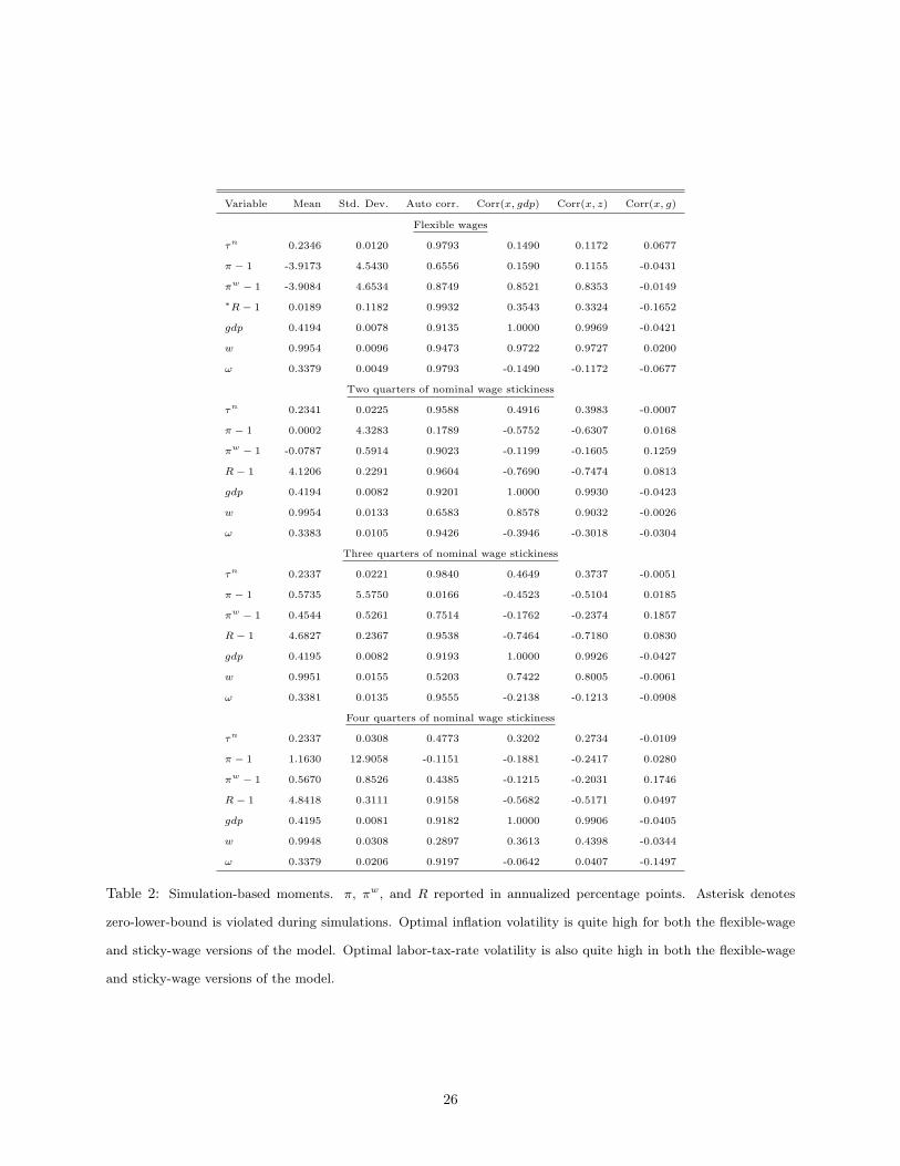
Table 2 presents simulation-based moments for the key policy variables for various degrees of nominal wage
rigidity. The top panel of Table 2 shows that if nominal wages are costless to adjust, the average level of
inflation is near the Friedman deflation (consistent with our steady-state results) and price inflation volatility,
at about 4.5 percent annualized, is quite high. The high volatility of inflation, well-known in Ramsey models,
is due to the fact that (large) state-contingent variations in inflation render nominally risk-free debt payments
state-contingent in real terms, thereby financing a large portion of innovations to the government budget
in a non-distortionary way. Thus, search and matching frictions in the labor market in and of themselves
do nothing to overturn this benchmark result. With flexible wages, nominal wage inflation is also quite
volatile. Coupled with volatile price inflation, the path for the real wage turns out to be relatively stable,
with a standard deviation of about 1 percent, much lower than the volatility of output, which has a standard
deviation of about 1.8 percent.17
If nominal wages are instead costly to adjust, nominal wage inflation is near zero with very low variability,
as the second, third, and fourth panels of Table 2 show. However — and this is our central finding — optimal
that the simulations are bounded away from the zero lower bound, they alter the Nash bargaining weight from the Hosioscondition as well as introduce a second source of inefficiency. They report (p. 188), however, that the introduction of thesefeatures just induce a level shift of variables without altering the basic cyclical properties of the model; the same is true in ourmodel.
17These standard deviations in percentage terms are simply equal to the raw standard deviations presented in Table 2 dividedby the means. We could have equivalently computed the standard deviation of the logged variables.
20

price inflation volatility remains quite high in the presence of costs of nominal wage rigidity. With two or
three quarters of nominally-rigid wages on average, price inflation volatility is still around five percent, little
changed from the fully-flexible case. With four quarters of wage stickiness, inflation volatility is actually
higher than in the fully-flexible case. These results are directly opposite the results in Chugh (2006), who finds
that even just two quarters of nominal wage rigidity (modeled through an identical Rotemberg-adjustment-
cost specification) lowers price inflation volatility by an order of magnitude.
Intuitively, the reason behind low and stable nominal wage inflation if ψ > 0 is easy to understand:
the Ramsey planner largely eliminates the direct resource cost associated with changes in nominal wages.
Absent direct resource costs stemming from nominal price changes, however, the tradeoff facing the Ramsey
planner in setting a state-contingent price inflation rate is the welfare loss due to any induced volatility in the
aggregate real wage versus the welfare gain due to the usual shock-absorption afforded by state-contingent
inflation. In contrast to a neoclassical model, the quantitative tradeoff resolves in favor of high inflation
volatility due to the presence of search frictions. An attendant consequence is that real wages become
volatile. As Table 2 shows, real wage volatility indeed rises as ψ rises, by about 50 percent moving from the
flexible-wage case to the case of three quarters of nominal wage stickiness.
Volatility in real wages, however, is not very undesirable from the Ramsey point of view in a search
and bargaining environment because, in the aggregate, the real wage is largely distributive in nature. In a
search and bargaining framework, the real wage plays two distinct roles. First, for job matches that have
already been formed, the actual — i.e., ex-post — real wage only divides the economic rents generated by
the formation of a labor-market match. Second, for currently-searching (but not-yet-matched) individuals,
the real wage is an allocative signal.18 Important to understand is that for currently-searching individuals,
it is the ex-ante — i.e., before employment relationships have been formed — real wage that matters. Given
that labor flows are a small fraction of the total employment stock, the aggregate real wage plays, as we
stated above, a largely distributive role. As such, the Ramsey planner, concerned with allocations and not
distributions, is not compelled to “stabilize” aggregate real wages over time. This is in direct contrast to
the mechanism underlying the results in Chugh (2006): there, real wage volatility is undesirable because the
18Although not the only allocative signal; rather, as is well-understood in search and matching models, it is aggregate markettightness — our variable θ — that is typically the most important variable governing efficiency.
21

labor market has neoclassical underpinnings, meaning that the real wage is allocative for all units of labor
because there is simply no distinction between ex-ante wages and ex-post wages. In a neoclassical labor
market, costs of nominal wage changes translate into a desire for stabilizing nominal prices out of a concern
for inducing a real wage path close to the efficient one. Thus emerges a central conclusion of our study: it
clearly matters for prescriptions regarding optimal inflation in what type of underlying environment — a
neoclassical labor market or a labor market with fundamental frictions — nominal wage rigidity is modeled.
Another important dimension along which policy dynamics differ sharply between our model and a basic
Ramsey model is tax-rate dynamics. As Table 2 shows, our model displays tax-rate variability that is an order
of magnitude larger than in a basic Ramsey model, regardless of whether or not nominal wages are costly to
adjust.19 Our intuition regarding why tax-rate variability is not as undesirable in the search and bargaining
model as in a neoclassical model is similar to the intuition behind inflation variability. In aggregate, after-tax
real wage variability has mostly distributive consequences rather then allocative consequences. It is easiest
to understand the mechanism for the case ψ = 0. Recall from expression (16) how ωt and τnt are linked
dynamically: in any period in which τnt is high, ωt is low, and this relationship is linear. The top left panel
of Figure 1, which scatters dynamic realizations of ωt and τnt from a representative simulation of our model,
confirms this. Thus, variations in the labor tax rate cause variations in parties’ effective bargaining shares,
which have effects on ex-ante search incentives and ex-post divisions of match rents. For ongoing matches,
tax-rate variability is non-distorting. The optimal tax rate thus trades off incentive effects against the ability
to raise revenue for the government in a non-distortionary way; quantitatively, this tradeoff is resolved in
favor of highly-volatile tax rates. The relationship between τnt and ωt is more difficult to see if ψ > 0, but
high tax-rate variability remains intact; as shown in Figure 1, the cyclical correlation between τnt and ωt is
still strongly negative.
The mechanism that leads to both highly-volatile tax rates and highly-volatile inflation rates is thus the
following. Policy volatility induces variations in bargaining shares. In turn, these volatile bargaining shares
affect search incentives for unmatched individuals, but only affect rents for matched individuals. A Ramsey
problem is all about raising revenue in the least distortionary way possible; raising revenues by affecting19Tax rate volatility does not arise because our overall model is excessively volatile: as we noted above and as can be seen in
Table 2, the coefficient of variation of total output is about 1.8 percent, in line with empirical evidence and with basic Ramseymodels.
22
rents is thus potentially a very attractive source of financing. A bargaining environment thus articulates
a novel dynamic policy channel about which a standard model is silent, namely the ability of policy to
respond to shocks by expropriating rents in a time-varying, state-contingent way. We refer parsimoniously
to this entire policy mechanism by saying that optimal policy exploits a dynamic bargaining power effect.
The dynamic bargaining power effect underpins the model’s predictions of both high tax-rate volatility and,
in the presence of sticky wages, high inflation volatility.
Because the labor search model is so well-suited to thinking about issues regarding unemployment, one
may wonder whether a Phillips Curve arises in our model. In the working paper version, we show that a
negative relationship between cyclical inflation rates and cyclical unemployment rates does arise under the
Ramsey equilibrium if wages are flexible. However, this Phillips relation is not a feature of optimal policy
with sticky nominal wages. A downward-sloping wage Phillips Curve is also not a feature of the optimal
policy.
Finally, we do not report our model’s predictions regarding the volatility of unemployment, vacancies,
and labor market tightness, a topic that has received much attention since Shimer (2005) and Hall (2005).
A thorough analysis of this aspect of our model is provided in the working paper version, but the upshot is
that, although the volatility of all three variables increase slightly as the costs of nominal wage adjustment
increase, optimal policy in and of itself does not offer any breakthroughs in understanding the volatility
puzzle.
To summarize our results on optimal stabilization policy, neither inflation variability nor tax-rate vari-
ability creates quantitatively-important distortions in our model because the variations in realized (after-tax)
real wages that they induce are largely isolated from determination of quantities. The results suggest that if
the realized real wage did affect allocations more directly, then the optimal degree of price inflation volatil-
ity may fall as the cost of nominal wage adjustment rises. In the working paper, this idea is pursued by
introducing an intensive margin of labor adjustment that potentially is affected by the realized real wage in
a similar manner as in a standard neoclassical model. The broad result is that inflation volatility result is
robust to the introduction of an intensive margin, although the precise quantitative results can depend on
the details of the hours-determination mechanism.
23
5 Conclusion
The goal of our study was to explore the implications of nominally-rigid wages on optimal policy in a
model featuring explicit bilateral relationships between workers and firms. The results turn out to be quite
different than in models with nominal rigidities in wages modeled in otherwise-neoclassical labor markets.
In a search and bargaining model, realized real wages play primarily a distributive role and are not as
critical for efficiency as they are in a labor market with standard neoclassical underpinnings. Thus, although
unanticipated fluctuations in inflation and the labor income tax rate cause unanticipated fluctuations in
(after-tax) real wages, job formation and production are largely unaffected. Our results give quantitative
voice to the conjecture, based on Barro’s (1979) critique and recently articulated in Goodfriend and King
(2001), that sticky nominal wages ought not to have much consequence for optimal monetary policy because
firms and workers in long-lived relationships have the proper incentives to neutralize any allocative effects.
This paper is also part of a larger project studying the policy implications of deep-rooted, non-Walrasian
frictions in goods markets, money markets, and labor markets. A central focus of this larger project has been
to think about what sorts of departures from typical Walrasian frameworks make consumer price inflation
stability an important goal of policy, but along the way we have uncovered other aspects of policy not evident
in standard models. In this paper, we characterized optimal policy when labor markets are non-Walrasian
but goods markets and money markets are standard. Aruoba and Chugh (2006) characterized optimal policy
when money markets are non-Walrasian but labor markets and goods markets are standard. Arseneau and
Chugh (2008) characterize optimal policy when goods markets are non-Walrasian but labor markets and
money markets are standard. One of the next topics on our research agenda is characterizing optimal policy
when multiple markets feature fundamental trading frictions.
24

Type of allocation Wage Rigidity R− 1 π − 1 τn gdp N v θ
Ramsey None 0 -3.9404 0.2350 0.4195 0.8748 0.1649 1.3167
Ramsey Two quarters 4.0649 -0.0357 0.2343 0.4195 0.8748 0.1649 1.3166
Ramsey Three quarters 4.6049 0.4831 0.2343 0.4196 0.8749 0.1650 1.3195
Ramsey Four quarters 4.7203 0.5939 0.2343 0.4197 0.8751 0.1652 1.3224
Social Planner — 0 -3.9404 0 0.4160 0.8674 0.1564 1.1791
Table 1: Steady-state policy and allocations. Inflation rate and interest rate reported in annualized percentage
points. For Social Planning problem, implied policy variables constructed residually using equilibrium conditions.
As costs of nominal wage adjustment rise above zero, the Ramsey inflation rate rises above the Friedman Rule and
becomes positive between two and three quarters of wage stickiness. The labor tax rate and real allocations are not
very sensitive to the cost adjustment parameter ψ.
25
Variable Mean Std. Dev. Auto corr. Corr(x, gdp) Corr(x, z) Corr(x, g)
Flexible wages
τn 0.2346 0.0120 0.9793 0.1490 0.1172 0.0677
π − 1 -3.9173 4.5430 0.6556 0.1590 0.1155 -0.0431
πw − 1 -3.9084 4.6534 0.8749 0.8521 0.8353 -0.0149
∗R− 1 0.0189 0.1182 0.9932 0.3543 0.3324 -0.1652
gdp 0.4194 0.0078 0.9135 1.0000 0.9969 -0.0421
w 0.9954 0.0096 0.9473 0.9722 0.9727 0.0200
ω 0.3379 0.0049 0.9793 -0.1490 -0.1172 -0.0677
Two quarters of nominal wage stickiness
τn 0.2341 0.0225 0.9588 0.4916 0.3983 -0.0007
π − 1 0.0002 4.3283 0.1789 -0.5752 -0.6307 0.0168
πw − 1 -0.0787 0.5914 0.9023 -0.1199 -0.1605 0.1259
R− 1 4.1206 0.2291 0.9604 -0.7690 -0.7474 0.0813
gdp 0.4194 0.0082 0.9201 1.0000 0.9930 -0.0423
w 0.9954 0.0133 0.6583 0.8578 0.9032 -0.0026
ω 0.3383 0.0105 0.9426 -0.3946 -0.3018 -0.0304
Three quarters of nominal wage stickiness
τn 0.2337 0.0221 0.9840 0.4649 0.3737 -0.0051
π − 1 0.5735 5.5750 0.0166 -0.4523 -0.5104 0.0185
πw − 1 0.4544 0.5261 0.7514 -0.1762 -0.2374 0.1857
R− 1 4.6827 0.2367 0.9538 -0.7464 -0.7180 0.0830
gdp 0.4195 0.0082 0.9193 1.0000 0.9926 -0.0427
w 0.9951 0.0155 0.5203 0.7422 0.8005 -0.0061
ω 0.3381 0.0135 0.9555 -0.2138 -0.1213 -0.0908
Four quarters of nominal wage stickiness
τn 0.2337 0.0308 0.4773 0.3202 0.2734 -0.0109
π − 1 1.1630 12.9058 -0.1151 -0.1881 -0.2417 0.0280
πw − 1 0.5670 0.8526 0.4385 -0.1215 -0.2031 0.1746
R− 1 4.8418 0.3111 0.9158 -0.5682 -0.5171 0.0497
gdp 0.4195 0.0081 0.9182 1.0000 0.9906 -0.0405
w 0.9948 0.0308 0.2897 0.3613 0.4398 -0.0344
ω 0.3379 0.0206 0.9197 -0.0642 0.0407 -0.1497
Table 2: Simulation-based moments. π, πw, and R reported in annualized percentage points. Asterisk denotes
zero-lower-bound is violated during simulations. Optimal inflation volatility is quite high for both the flexible-wage
and sticky-wage versions of the model. Optimal labor-tax-rate volatility is also quite high in both the flexible-wage
and sticky-wage versions of the model.
26

0.15 0.2 0.25 0.3 0.35 0.40.24
0.26
0.28
0.3
0.32
0.34
0.364 quarters
τn
ω
0.2 0.25 0.3 0.35 0.40.26
0.28
0.3
0.32
0.34
0.36
τn
ω
3 quarters
0.22 0.24 0.26 0.28 0.3 0.320.28
0.29
0.3
0.31
0.32
0.33
0.34
0.352 quarters
τn
ω
0.2 0.21 0.22 0.23 0.24 0.250.335
0.34
0.345
0.35
0.355Flexible
ω
τn
Figure 1: Dynamic relationship between worker’s effective bargaining power (ω) and labor tax rate under the Ramsey
policy for various degrees of nominal wage rigidity. With zero costs of wage adjustment, the relationship is inverse
linear, as can be shown analytically. With positive costs of wage adjustment, the relationship is less tight but still
clearly linear. Thus, higher labor tax rates drive down workers’ effective bargaining power.
27
References
Andolfatto, David. 1996. “Business Cycles and Labor-Market Search.” American Economic Review,
Vol. 86, pp. 112-132.
Aiyagari, S. Rao, Albert Marcet, Thomas J, Sargent, and Juha Seppala. 2002. “Optimal
Taxation without State-Contingent Debt.” Journal of Political Economy, Vol. 110, pp. 1220-1254.
Arseneau, David M. and Sanjay K. Chugh. 2006. “Ramsey Meets Hosios: The Optimal Capital Tax
and Labor Market Efficiency.” International Finance Discussion Paper no. 870. , Board of Governors
of the Federal Reserve System.
Arseneau, David M. and Sanjay K. Chugh. 2007. “Optimal Fiscal and Monetary Policy with Costly
Wage Bargaining.” International Finance Discussion Paper no. 893 , Board of Governors of the Federal
Reserve System.
Arseneau, David M. and Sanjay K. Chugh. 2008. “Optimal Fiscal and Monetary Policy in Customer
Markets.” International Finance Discussion Paper no. 919 , Board of Governors of the Federal Reserve
System.
Aruoba, S. Boragan and Sanjay K. Chugh. 2006. “Optimal Fiscal and Monetary Policy When
Money is Essential.” International Finance Discussion Paper no. 880. , Board of Governors of the
Federal Reserve System.
Barro, Robert J. 1977. “Long-Term Contracting, Sticky Prices, and Monetary Policy.” Journal of
Monetary Economics, Vol. 3, pp. 305-316.
Blanchard, Olivier and Peter Diamond. 1989. “The Beveridge Curve.” Brookings Papers on
Economic Activity, Vol. 1, pp. 1-76.
Blanchard, Olivier and Jordi Gali. 2006. “A New Keynesian Model with Unemployment.” MIT.
Blanchard, Olivier and Jordi Gali. 2007. “Real Wage Rigidities and the New Keynesian Model.”
Journal of Money, Credit, and Banking, Vol. 39, pp. 35-65.
Chari, V.V., Lawrence Christiano, and Patrick Kehoe. 1991. “Optimal Fiscal and Monetary
Policy: Some Recent Results.” Journal of Money, Credit, and Banking, Vol. 23, pp. 519-539.
Christoffel, Kai and Tobias Linzert. 2005. “The Role of Real Wage Rigidity and Labor Market
28

Frictions for Unemployment and Inflation Dynamics.” European Central Bank.
Chugh, Sanjay K. 2006. “Optimal Fiscal and Monetary Policy with Sticky Wages and Sticky Prices.”
Review of Economi Dynamics, Vol. 9, pp. 683-714.
Chugh, Sanjay K. 2007. “Optimal Inflation Persistence: Ramsey Taxation with Capital and Habits.”
Journal of Monetary Economics, Vol. 54, pp. 1809-1836.
Chugh, Sanjay K. 2008. “Does the Timing of the Cash-in-Advance Constraint Matter for Optimal Fiscal
and Monetary Policy?.” Macroeconomic Dynamics. Forthcoming.
Cooley, Thomas F. and Vincenzo Quadrini. 2004. “Optimal Monetary Policy in a Phillips-Curve
World.” Journal of Economic Theory, Vol. 118, pp. 174-208.
Domeij, David. 2005. “Optimal Capital Taxation and Labor Market Search.” Review of Economic
Dynamics, Vol. 8, pp. 623-650.
Erceg, Christoper J., Dale W. Henderson, and Andrew Levin. 2000. “Optimal Monetary Policy
with Staggered Wage and Price Contracts.” Journal of Monetary Economics, Vol. 46, pp. 281-313.
Faia, Ester. 2008. “Optimal Monetary Policy Rules with Labor Market Frictions.” Journal of Economic
Dynamics and Control, Vol. 32, pp. 1600-1621.
Gertler, Mark and Antonella Trigari. 2006. “Unemployment Fluctuations with Staggered Nash
Bargaining.” New York University.
Goodfriend, Marvin and Robert G. King. 2001. “The Case for Price Stability.” NBER Working
Paper 8423.
Hall, Robert E. 2005. “Equilibrium Wage Stickiness.” American Economic Review, Vol. 95, pp. 50-65.
Hosios, Arthur J. 1990. “On the Efficiency of Matching and Related Models of Search and Unemploy-
ment.” Review of Economic Studies, Vol. 57, pp. 279-298.
Krause, Michael U. and Thomas A. Lubik. 2007. “The (Ir)relevance of Real Wage Rigidity in the
New Keynesian Model with Search Frictions.” Journal of Monetary Economics, Vol. 55, pp. 706-727.
Lucas, Robert E. Jr. and Nancy L. Stokey. 1983. “Optimal Fiscal and Monetary Policy in an
Economy Without Capital.” Journal of Monetary Economics, Vol. 12, pp. 55-93.
Merz, Monika. 1995. “Search in the Labor Market and the Real Business Cycle.” Journal of Monetary
29
Economics, Vol. 36, pp. 269-300.
Pissarides, Christopher A. 2000. Equilibrium Unemployment Theory. MIT Press.
Schmitt-Grohe, Stephanie and Martin Uribe. 2004a. “Optimal Fiscal and Monetary Policy Under
Sticky Prices.” Journal of Economic Theory, Vol. 114, pp. 198-230.
Schmitt-Grohe, Stephanie and Martin Uribe. 2004b. “Solving Dynamic General Equilibrium
Models Using a Second-Order Approximation to the Policy Function.” Journal of Economic Dynamics
and Control, Vol. 28, pp. 755-775.
Schmitt-Grohe, Stephanie and Martin Uribe. 2005. “Optimal Fiscal and Monetary Policy in a
Medium-Scale Macroeconomic Model.” NBER Macroeconomics Annual 2005.
Scott, Andrew. 2007. “Optimal Taxation and OECD Labor Taxes.” Journal of Monetary Economics,
Vol. 54, pp. 924-944.
Shimer, Robert. 2005. “The Cyclical Behavior of Equilibrium Unemployment and Vacancies.” American
Economic Review, Vol. 95, pp. 25-49.
Siu, Henry E. 2004. “Optimal Fiscal and Monetary Policy with Sticky Prices.” Journal of Monetary
Economics, Vol. 51, pp. 576-607.
Svensson, Lars E. O. 1985. “Money and Asset Prices in a Cash-in-Advance Economy.” Journal of
Political Economy, Vol. 93, pp. 919-944.
Thomas, Carlos. 2008. “Search and Matching Frictions and Optimal Monetary Policy.” Journal of
Monetary Economics. Forthcoming.
Trigari, Antonella. 2006. “The Role of Search Frictions and Bargaining for Inflation Dynamics.”
Bocconi University.
Werning Ivan. 2007. “Optimal Fiscal Policy with Redistribution.” Quarterly Journal of Economics, Vol.
122, pp. 925-967.
30