Optimal Control for the Trajectory Planning of Micro Airships*

Charles Blouin1 and Eric Lanteigne1 and Wail Gueaieb2

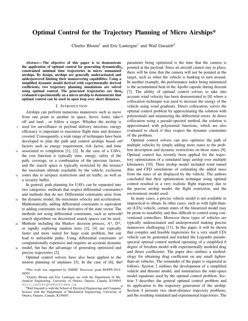
Abstract— The objective of this paper is to demonstratethe application of optimal control for generating dynamicallyconstrained minimal time trajectories in micro unmannedairships. By design, airships are generally underactuated andunderpowered limiting their maneuvering capabilities. Using asimplified dynamic model derived with experimentally derivedcoefficients, two trajectory planning simulations are solvedusing optimal control. The generated trajectories are thenevaluated experimentally on a micro airship to demonstrate thatoptimal control can be used in open loop over short distances.

I. INTRODUCTION

Airships can perform numerous maneuvers such as movefrom one point to another in space, hover, loiter, take-off and land , or follow a target. Whether the airship isused for surveillance or payload delivery missions, energy5

efficiency is important to maximize flight time and distancecovered. Consequently, a wide range of techniques have beendeveloped to plan the path and control airships based onfactors such as energy requirement, risk factor, and timeassociated to completion [1], [2]. In the case of a UAVs,10

the cost function is typically time, energy, safety of thepath, coverage, or a combination of the previous factors,and the search space is typically restricted by the terrain,the maximum altitude reachable by the vehicle, exclusionzones due to airspace restrictions and air traffic, as well as15

a security buffer.In general, path planning for UAVs can be separated into

two categories: methods that respect differential constraints,and methods that do not. Differential constraints arise fromthe dynamic model, the maximum velocity and acceleration.20

Mathematically, adding differential constraints is equivalentto adding constraints on the derivative of the state vector. Themethods not using differential constraints, such as networksearch algorithms on discretized search spaces can be used.Methods including the Markov decision process, A*, D*,25

or rapidly exploring random trees [3], [4] are typicallyfaster and more suited for large scale problem, but canlead to unfeasible paths. Using differential constraints iscomputationally expensive and requires an accurate dynamicmodel, but has the advantage of generating optimized and30

precise trajectories [2].Optimal control solvers have also been applied to the

motion planning of airplanes [5]. In the case of [6], the

*This work was supported by NSERC Discovery grant RGPIN-2014-04501

1Charles Blouin and Eric Lanteigne are with the Department of Me-chanical Engineering, University of Ottawa, Ontario, Canada, K1N6N5eric.lanteigne@uottawa.ca

2Wail Gueaieb is with the School of Electrical Engineering and ComputerScience with the Department of Mechanical Engineering, University ofOttawa, Ontario, Canada, K1N6N5

parameter being optimized is the time that the camera ispointed at the payload. Since an aircraft cannot stay in place,35

there will be time that the camera will not be pointed at thetarget, such as when the vehicle is banking to turn around.In another example, the performance index being minimizedis the accumulated heat in the Apollo capsule during descent[7]. The ability of optimal control solvers to take into40

account wind velocity has been demonstrated in [8] where acollocation technique was used to increase the energy of thevehicle using wind gradients. Direct collocation, solves theoptimal control problem by approximating the solution withpolynomials and minimizing the differential errors. In direct45

collocation using a pseudo-spectral method, the solution isapproximated with polynomial functions, which are alsoevaluated to check if they respect the dynamic constraintsof the problem.

Optimal control solvers can also optimize the path of50

multiple vehicles by simply adding more states to the prob-lem description and dynamic restrictions on those states [9].Optimal control has recently been applied for the trajec-tory optimization of a simulated large airship over multiplekilometers [10]. Their airship model included wind tunnel55

data and CFD simulations of estimating the added massfrom the mass of air displaced by the vehicle. The authorsconcluded that their optimization technique using optimalcontrol resulted in a very realistic flight trajectory due tothe precise airship model, the flight restriction, and the60

environment model used.In many cases, a precise vehicle model is not available or

impractical to obtain. In other cases, such as with light-than-air (LTA) vehicle, certain states of the linearized model maybe prone to instability and thus difficult to control using con-65

ventional controllers. Moreover these types of vehicles aretypically underactuated and underpowered making precisemaneuvers challenging [11]. In this paper, it will be shownthat complex and feasible trajectories for a very small LTAvehicle can be generated and tracked the Legendre pseudo-70

spectral optimal control method operating of a simplified 6degree of freedom model with experimentally modeled dragand thrust coefficients. The paper also outlines a method-ology for obtaining drag coefficient on any small lighter-than-air vehicles. The remainder of the paper is organized as75

follows. Section 2 outlines the development of a simplifiedvehicle and thruster model, and summarizes the state-spacemodel equations used by the optimal control problem. Sec-tion 3 describes the general optimal control problem andits application to the trajectory generation of the airship.80

Section 4 presents two short-distance trajectory problems,and the resulting simulated and experimental trajectories. The

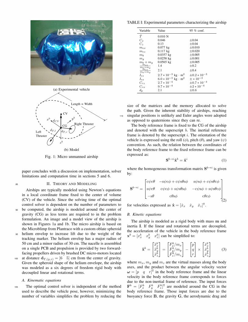
(a) Experimental vehicle

CV

Left

Length = Width

dCV

dT,r

CG

xb yb

zb

Right Thruster

dT,l

Thruster

(b) Model

Fig. 1: Micro unmanned airship

paper concludes with a discussion on implementation, solverlimitations and computation time in sections 5 and 6.

II. THEORY AND MODELING85

Airships are typically modeled using Newton’s equationsin a local coordinate frame fixed to the center of volume(CV) of the vehicle. Since the solving time of the optimalcontrol solver is dependent on the number of parameters tobe computed, the airship is modeled around the center of90

gravity (CG) as less terms are required to in the problemformulation. An image and a model view of the airship isshown in Figures 1a and 1b. The micro airship is based onthe Microblimp from Plantraco with a custom oblate spheroidhelium envelop to increase lift due to the weight of the95

tracking marker. The helium envelop has a major radius of50 cm and a minor radius of 30 cm. The nacelle is assembledon a single PCB and propulsion is provided by two forward-facing propellers driven by brushed DC micro-motors locatedat distance dT,(y,z) = [6 5] cm from the center of gravity.100

Given the spheroid shape of the helium envelope, the airshipwas modeled as a six degrees of freedom rigid body withdecoupled linear and rotational terms.

A. Kinematic equations

The optimal control solver is independent of the method105

used to describe the vehicle pose, however, minimizing thenumber of variables simplifies the problem by reducing the

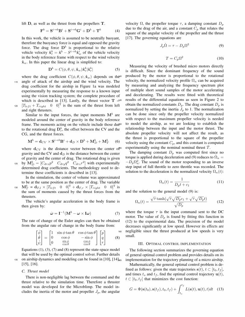
TABLE I: Experimental parameters characterizing the airship

Variable Value 95 % conf.

T 0.010 NCx 0.046 ±0.04Cz 0.13 ±0.04mex 0.077 kg ±0.010mez 0.117 kg ±0.020mb 0.0357 kg ±0.005mg 0.0258 kg ±0.001mb +mg 0.0565 kg ±0.005

mexmb+mg

1.4 ±0.2mez

mb+mg2.1 ±0.4

Iez 2.7 ∗ 10−3 kg · m2 ±0.2 ∗ 10−3

Iex 6.0 ∗ 10−3 kg · m2 ± ∗ 10−3

Crz 2.7 ∗ 10−4 ±0.7 ∗ 10−4

Crx 9.7 ∗ 10−4 ±2 ∗ 10−4

dp 2.1 ±0.6

size of the matrices and the memory allocated to solvethe path. Given the inherent stability of airships, reachingsingular positions is unlikely and Euler angles were adopted110

as opposed to quaternions since they can re.The body reference frame is fixed to the CG of the airship

and denoted with the superscript b. The inertial referenceframe is denoted by the superscript i. The orientation of thevehicle is expressed using the roll (φ), pitch (θ), and yaw (ψ)convention. As such, the relation between the coordinates ofthe body reference frame to the fixed reference frame can beexpressed as:

Sb→ixb = xi (1)

where the homogeneous transformation matrix Sb→i is givenby:

Sb→i =

cψcθ −sψcφ+ cψsθsφ sψsφ+ cψsθcφ

sψcθ cψcφ+ sψsθsφ −cψsφ+ sψsθcφ

−sθ cθsφ cθcφ

(2)

for velocities expressed as x = [xx xy xz]T.

B. Kinetic equations

The airship is modeled as a rigid body with mass m andinertia I. If the linear and rotational terms are decoupled,the acceleration of the vehicle in the body reference framexb = [xbx xby xbz] can be simplified to:

xb =

xbxxbyxbz

=

F bx/mx

F by/my

F bz /mz

−pqr

×xbxxbyxbz

(3)

where mx, my and mz are the virtual masses along the bodyaxes, and the product between the angular velocity vectorω = [p q r]T in the body reference frame and the linearvelocity in the body reference frame corresponds to forcesdue to the non-inertial frame of reference. The input forcesFb = [F bx F by F bz ]T are modeled around the CG in thebody reference frame. Those input forces are due to thebuoyancy force B, the gravity G, the aerodynamic drag and

lift D, as well as the thrust from the propellers T.

Fb = Si→bBi + Si→bGi + Db + Tb (4)

In this work, the vehicle is assumed to be neutrally buoyant,therefore the buoyancy force is equal and opposed the gravityforce. The drag force Db is proportional to the relativevehicle velocity xbr = xb − Si→bxiw of the vehicle velocityin the body reference frame with respect to the wind velocityxw. In this paper the linear drag is simplified to:

Db = C(φ, θ, ψ, xw)xbr|xbr| (5)

where the drag coefficient C(φ, θ, ψ, xw) depends on theangle of attack of the airship and the wind velocity. The115

drag coefficient for the airship in Figure 1a was modeledexperimentally by measuring the response to a known inputusing the vision tracking system; the complete procedure ofwhich is described in [13]. Lastly, the thrust vector T =[Tleft + Tright 0 0]T is the sum of the thrust from left120

and right thrusters.Similar to the input forces, the input moments Mb are

modeled around the center of gravity in the body referenceframe. The moments acting on the vehicle include those dueto the rotational drag Db

r, the offset between the CV and theCG, and the thrust forces.

Mb = dCV × Si→bBi + dD ×Db + MbD + Mb

T (6)

where dCV is the distance vector between the center ofgravity and the CV and dD is the distance between the centerof gravity and the center of drag. The rotational drag is givenby Mb

D = [Cdrxp2 Cdryq

2 Cdrzr2] with experimentally125

determined drag coefficients. The methodology used to de-termine these coefficients is described in [13].

In the simulation, the center of volume was approximatedto be at the same position as the center of drag. The variableMb

T = dT,l × [Tleft 0 0]T + dT,r × [Tright 0 0]T is130

the sum of moments caused by the thrust forces from thethrusters.

The vehicle’s angular acceleration in the body frame isthen given by:

ω = I−1(Mb − ω × Iω) (7)

The rate of change of the Euler angles can then be obtainedfrom the angular rate of change in the body frame from:φθ

ψ

=

1 sinφ tan θ cosφ tan θ0 cosφ − sinφ

0 sinφcos θ

cosφcos θ

pqr

(8)

Equations (1), (3), (7) and (8) represent the state-space modelthat will be used by the optimal control solver. Further detailson airship dynamics and modeling can be found in [10], [14],135

[15], [16].

C. Thrust model

There is non-negligible lag between the command and thethrust relative to the simulation time. Therefore a thrustermodel was developed for the Microblimp. The model in-cludes the inertia of the motor and propeller Jp, the angular

velocity Ω, the propeller torque τ , a damping constant Dp

due to the drag of the air, and a constant Cp that relates thesquare of the angular velocity of the propeller and the thrust[17]. The governing equations are

JpΩ = τ −DpΩ2 (9)

T = CpΩ2 (10)

Measuring the velocity of brushed micro motors directlyis difficult. Since the dominant frequency of the soundproduced by the motor is proportional to the rotational140

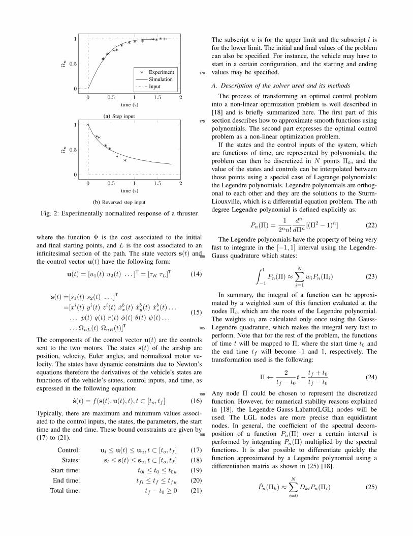
velocity, the normalized velocity profile Ωn can be acquiredby measuring and analyzing the frequency spectrum plotof multiple short sound samples of the motor acceleratingand decelerating. The results were fitted with theoreticalresults of the differential equations as seen in Figure 2 to145

obtain the normalized constants Dp. The drag constant Dp isnormalized by setting the inertia Jp to 1. The normalizationcan be done since only the propeller velocity normalizedwith respect to the maximum propeller velocity is neededto model the airship, as we are looking to establish the150

relationship between the input and the motor thrust. Theabsolute propeller velocity will not affect the result, asthe thrust is proportional to the square of the propellervelocity using the constant Cp, and this constant is computedexperimentally using the nominal nominal thrust T .155

The damping constant Dp was computed first since notorque is applied during deceleration and (9) reduces to Ωn =−DpΩ

2n. The sound of the motor responding to an inverse

step input of full throttle to zero throttle was recorded. Thesolution to the deceleration is the normalized velocity Ωn(t):

Ωn(t) =1

Dpt+ c1(11)

and the solution to the general model (9) is:

Ωn(t) =

√τ tanh(

√τ√Dpc1 +

√τ√Dpt)√

Dp

(12)

where the torque τ is the input command sent to the DCmotor. The value of Dp is found by fitting this function in(12) to the experimental data. The precision of the modeldecreases significantly at low speed. However its effects arenegligible since the thrust produced at low speeds is very160

small.

III. OPTIMAL CONTROL IMPLEMENTATION

The following section summarizes the governing equationof general optimal control problem and provides details on itsimplementation for the trajectory planning of a micro airship.165

Mathematically, the general optimal control problem is de-fined as follows: given the state trajectories s(t), t ⊂ [t0, tf ],and times to and tf , find the optimal control trajectory u(t),t ⊂ [t0, tf ] that minimizes the cost function:

G = Φ(s(t0), s(tf ), t0, tf ) +

∫ tf

to

L(s(t),u(t), t)dt (13)

0 0.5 1 1.5 2

0

0.5

1

time (s)

Ωn

ExperimentSimulationInput

(a) Step input

0 0.5 1 1.5 2

0

0.5

1

time (s)

Ωn

(b) Reversed step input

Fig. 2: Experimentally normalized response of a thruster

where the function Φ is the cost associated to the initialand final starting points, and L is the cost associated to aninfinitesimal section of the path. The state vectors s(t) andthe control vector u(t) have the following form:

u(t) = [u1(t) u2(t) . . . ]T = [τR τL]T (14)

s(t) =[s1(t) s2(t) . . . ]T

=[xi(t) yi(t) zi(t) xbx(t) xby(t) xbz(t) . . .

. . . p(t) q(t) r(t) φ(t) θ(t) ψ(t) . . .

. . .ΩnL(t) ΩnR(t)]T

(15)

The components of the control vector u(t) are the controlssent to the two motors. The states s(t) of the airship areposition, velocity, Euler angles, and normalized motor ve-locity. The states have dynamic constraints due to Newton’sequations therefore the derivatives of the vehicle’s states arefunctions of the vehicle’s states, control inputs, and time, asexpressed in the following equation:

s(t) = f(s(t),u(t), t), t ⊂ [to, tf ] (16)

Typically, there are maximum and minimum values associ-ated to the control inputs, the states, the parameters, the starttime and the end time. These bound constraints are given by(17) to (21).

Control: ul ≤ u(t) ≤ uu, t ⊂ [to, tf ] (17)States: sl ≤ s(t) ≤ su, t ⊂ [to, tf ] (18)

Start time: t0l ≤ t0 ≤ t0u (19)End time: tfl ≤ tf ≤ tfu (20)

Total time: tf − t0 ≥ 0 (21)

The subscript u is for the upper limit and the subscript l isfor the lower limit. The initial and final values of the problemcan also be specified. For instance, the vehicle may have tostart in a certain configuration, and the starting and endingvalues may be specified.170

A. Description of the solver used and its methods

The process of transforming an optimal control probleminto a non-linear optimization problem is well described in[18] and is briefly summarized here. The first part of thissection describes how to approximate smooth functions using175

polynomials. The second part expresses the optimal controlproblem as a non-linear optimization problem.

If the states and the control inputs of the system, whichare functions of time, are represented by polynomials, theproblem can then be discretized in N points Πk, and thevalue of the states and controls can be interpolated betweenthose points using a special case of Lagrange polynomials:the Legendre polynomials. Legendre polynomials are orthog-onal to each other and they are the solutions to the Sturm-Liouxville, which is a differential equation problem. The nthdegree Legendre polynomial is defined explicitly as:

Pn(Π) =1

2nn!

dn

dΠn[(Π2 − 1)n] (22)

The Legendre polynomials have the property of being veryfast to integrate in the [−1, 1] interval using the Legendre-Gauss quadrature which states:180 ∫ 1

−1Pn(Π) ≈

N∑i=1

wiPn(Πi) (23)

In summary, the integral of a function can be approxi-mated by a weighted sum of this function evaluated at thenodes Πi, which are the roots of the Legendre polynomial.The weights wi are calculated only once using the Gauss-Legendre quadrature, which makes the integral very fast to185

perform. Note that for the rest of the problem, the functionsof time t will be mapped to Π, where the start time t0 andthe end time tf will become -1 and 1, respectively. Thetransformation used is the following:

Π← 2

tf − t0t− tf + t0

tf − t0(24)

Any node Π could be chosen to represent the discretized190

function. However, for numerical stability reasons explainedin [18], the Legendre-Gauss-Labatto(LGL) nodes will beused. The LGL nodes are more precise than equidistantnodes. In general, the coefficient of the spectral decom-position of a function Pn(Π) over a certain interval is195

performed by integrating Pn(Π) multiplied by the spectralfunctions. It is also possible to differentiate quickly thefunction approximated by a Legendre polynomial using adifferentiation matrix as shown in (25) [18].

Pn(Πk) ≈N∑i=0

DkiPn(Πi) (25)

Consequently, the function to being optimized can berewritten as

G = φ(s(−1), s(1), t0, tf ) +tf − t0

2

∫ 1

−1L(s(Π),u(Π),Πdt

≈ φ(sN (−1), sN (1), t0, tf ) + . . .

tf − t02

N∑k=0

[L(sN (Πk),uN (Πk),Πk

]ωkdt

(26)

In the previous equation, sN and uN are the states and200

the control inputs approximating the exact solution withLegendre polynomials of order N . For smooth functions, theintegral can be approximated with very few points accurately.In the case of an airship, the performance index G willtypically be the time, the power required, or a combination205

of both, such as in [19].The solver will minimize the performance index while

respecting the differential constraints imposed on sN , sN

and uN .The vector representing the problem is y:210

y =[u s t0 tf

]T(27)

Finally, the minimization problem is solved by the non-linear optimizer IPOPT [20]. The non-linear optimizer trans-forms the problem into a linear algebra problem.

miny

G(y) (28)

subject to:Hl < H(y) < Hu (29)

yl < y < yu (30)

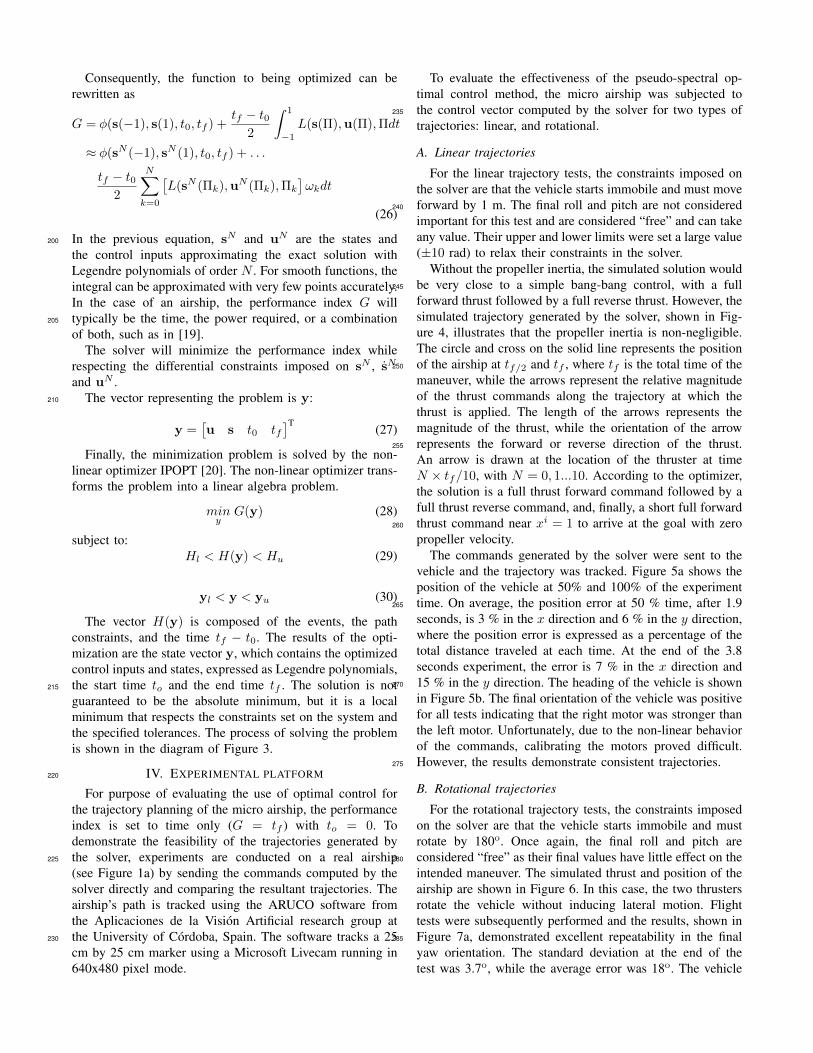
The vector H(y) is composed of the events, the pathconstraints, and the time tf − t0. The results of the opti-mization are the state vector y, which contains the optimizedcontrol inputs and states, expressed as Legendre polynomials,the start time to and the end time tf . The solution is not215

guaranteed to be the absolute minimum, but it is a localminimum that respects the constraints set on the system andthe specified tolerances. The process of solving the problemis shown in the diagram of Figure 3.

IV. EXPERIMENTAL PLATFORM220

For purpose of evaluating the use of optimal control forthe trajectory planning of the micro airship, the performanceindex is set to time only (G = tf ) with to = 0. Todemonstrate the feasibility of the trajectories generated bythe solver, experiments are conducted on a real airship225

(see Figure 1a) by sending the commands computed by thesolver directly and comparing the resultant trajectories. Theairship’s path is tracked using the ARUCO software fromthe Aplicaciones de la Vision Artificial research group atthe University of Cordoba, Spain. The software tracks a 25230

cm by 25 cm marker using a Microsoft Livecam running in640x480 pixel mode.

To evaluate the effectiveness of the pseudo-spectral op-timal control method, the micro airship was subjected tothe control vector computed by the solver for two types of235

trajectories: linear, and rotational.

A. Linear trajectories

For the linear trajectory tests, the constraints imposed onthe solver are that the vehicle starts immobile and must moveforward by 1 m. The final roll and pitch are not considered240

important for this test and are considered “free” and can takeany value. Their upper and lower limits were set a large value(±10 rad) to relax their constraints in the solver.

Without the propeller inertia, the simulated solution wouldbe very close to a simple bang-bang control, with a full245

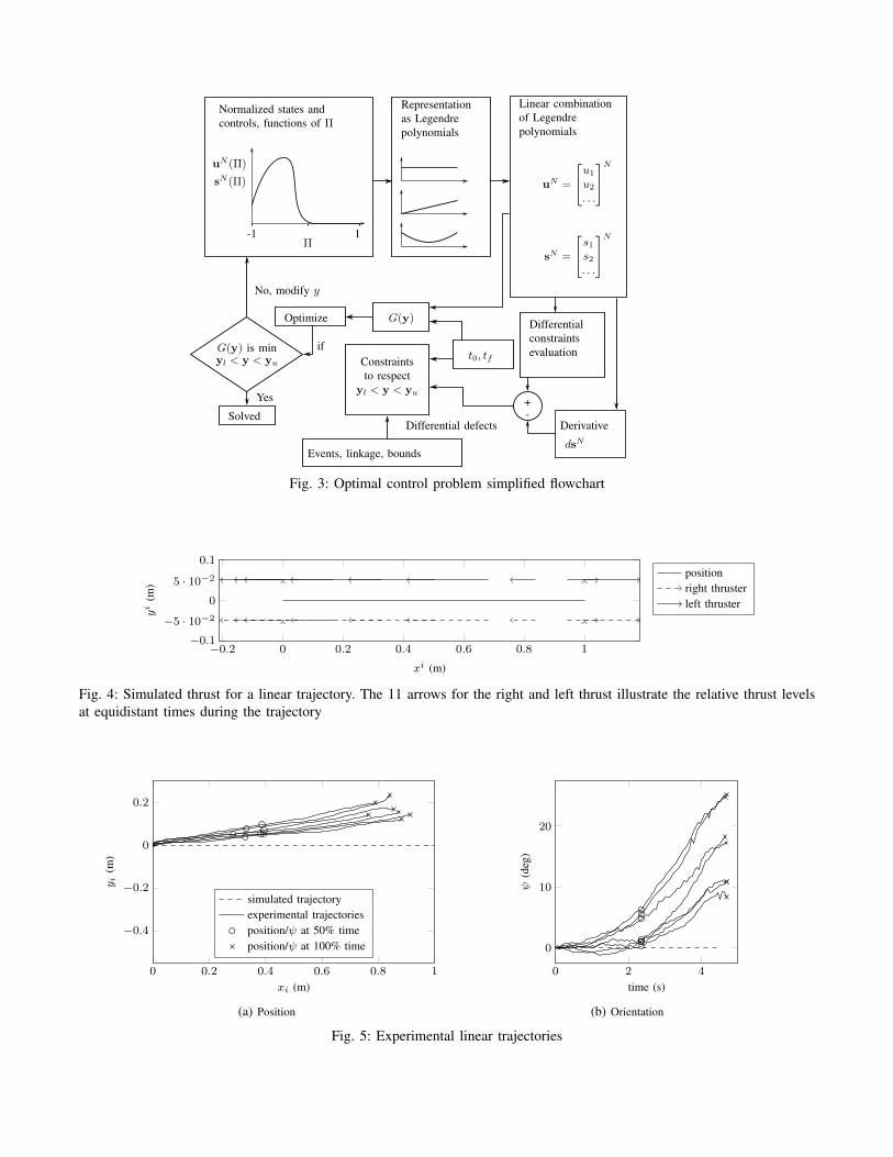
forward thrust followed by a full reverse thrust. However, thesimulated trajectory generated by the solver, shown in Fig-ure 4, illustrates that the propeller inertia is non-negligible.The circle and cross on the solid line represents the positionof the airship at tf/2 and tf , where tf is the total time of the250

maneuver, while the arrows represent the relative magnitudeof the thrust commands along the trajectory at which thethrust is applied. The length of the arrows represents themagnitude of the thrust, while the orientation of the arrowrepresents the forward or reverse direction of the thrust.255

An arrow is drawn at the location of the thruster at timeN × tf/10, with N = 0, 1...10. According to the optimizer,the solution is a full thrust forward command followed by afull thrust reverse command, and, finally, a short full forwardthrust command near xi = 1 to arrive at the goal with zero260

propeller velocity.The commands generated by the solver were sent to the

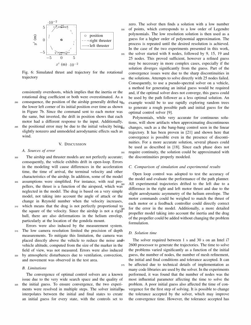
vehicle and the trajectory was tracked. Figure 5a shows theposition of the vehicle at 50% and 100% of the experimenttime. On average, the position error at 50 % time, after 1.9265

seconds, is 3 % in the x direction and 6 % in the y direction,where the position error is expressed as a percentage of thetotal distance traveled at each time. At the end of the 3.8seconds experiment, the error is 7 % in the x direction and15 % in the y direction. The heading of the vehicle is shown270

in Figure 5b. The final orientation of the vehicle was positivefor all tests indicating that the right motor was stronger thanthe left motor. Unfortunately, due to the non-linear behaviorof the commands, calibrating the motors proved difficult.However, the results demonstrate consistent trajectories.275

B. Rotational trajectories

For the rotational trajectory tests, the constraints imposedon the solver are that the vehicle starts immobile and mustrotate by 180o. Once again, the final roll and pitch areconsidered “free” as their final values have little effect on the280

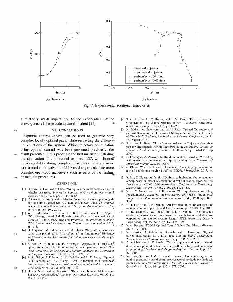
intended maneuver. The simulated thrust and position of theairship are shown in Figure 6. In this case, the two thrustersrotate the vehicle without inducing lateral motion. Flighttests were subsequently performed and the results, shown inFigure 7a, demonstrated excellent repeatability in the final285

yaw orientation. The standard deviation at the end of thetest was 3.7o, while the average error was 18o. The vehicle

Derivative

Optimize

sN =

s1s2. . .

N

Normalized states andcontrols, functions of Π

Representationas Legendrepolynomials

Linear combinationof Legendrepolynomials

Π

sN (Π)

uN (Π)

-1 1

uN =

u1u2. . .

N

dsN

Differentialconstraintsevaluation

+-

G(y)

t0, tf

Differential defects

Constraintsto respect

yl < y < yu

Events, linkage, bounds

yl < y < yu

Yes

No, modify y

if

Solved

G(y) is min

Fig. 3: Optimal control problem simplified flowchart

−0.2 0 0.2 0.4 0.6 0.8 1−0.1

−5 · 10−2

0

5 · 10−2

0.1

xi (m)

yi

(m)

positionright thrusterleft thruster

Fig. 4: Simulated thrust for a linear trajectory. The 11 arrows for the right and left thrust illustrate the relative thrust levelsat equidistant times during the trajectory

0 0.2 0.4 0.6 0.8 1

−0.4

−0.2

0

0.2

xi (m)

yi

(m)

simulated trajectoryexperimental trajectoriesposition/ψ at 50% timeposition/ψ at 100% time

(a) Position

0 2 4

0

10

20

time (s)

ψ(d

eg)

(b) Orientation

Fig. 5: Experimental linear trajectories

−5 0 5

·10−2

−5

0

5·10−2

xi (m)

yi

(m) position

right thrusterleft thruster

Fig. 6: Simulated thrust and trajectory for the rotationaltrajectory

consistently overshoots, which implies that the inertia or therotational drag coefficient or both were overestimated. As aconsequence, the position of the airship generally drifted to290

the lower left corner of its initial position over time as shownin Figure 7b. Since the command sent to each motor wasthe same, but inverted, the drift in position shows that eachmotor had a different response to the input. Additionally,the positional error may be due to the initial velocity being295

slightly nonzero and unmodeled aerodynamic effects such aswind.

V. DISCUSSION

A. Sources of error

The airship and thruster models are not perfectly accurate;300

consequently, the vehicle exhibits drift in open-loop. Errorsin the modeling will cause differences in the accelerationtime, the time of arrival, the terminal velocity and othercharacteristics of the airship. In addition, some of the modelassumptions were simplified. For instance, with real pro-305

pellers, the thrust is a function of the airspeed, which wasneglected in the model. The drag is based on a very simplemodel, not taking into account the angle of attack or thechange in Reynold number when the velocity increases,which means that the drag is not perfectly proportional to310

the square of the velocity. Since the airship is not a rigidhull, there are also deformations in the helium envelop,particularly at the location of the gondola mount.

Errors were also induced by the measurement system.The low camera resolution limited the precision of depth315

measurements. To mitigate this limitation, the camera wasplaced directly above the vehicle to reduce the noise andvehicle altitude, computed from the size of the marker in thefield of view, was not measured. Errors were also inducedby atmospheric disturbances due to ventilation, convection,320

and movement was observed in the test area.

B. Limitations

The convergence of optimal control solvers are a knownissue due to the very wide search space and the quality ofthe initial guess. To ensure convergence, the two experi-325

ments were resolved in multiple steps. The solver initiallyinterpolates between the initial and final states to createan initial guess for every state, with the controls set to

zero. The solver then finds a solution with a low numberof points, which corresponds to a low order of Legendre330

polynomials. The low resolution solution is then used as aguess for a higher order of polynomial approximation. Theprocess is repeated until the desired resolution is achieved.In the case of the two experiments presented in this work,the solver started with 8 nodes, followed by 9, 15, 19 and335

25 nodes. This proved sufficient, however a refined guessmay be necessary in more complex cases, especially if thesolution diverges significantly from the guess. Part of theconvergence issues were due to the sharp discontinuities inthe solutions. Attempts to solve directly with 25 nodes failed.340

Consequently, to use a pseudo-spectral solver on a vehicle,a method for generating an initial guess would be requiredand, if the optimal solver does not converge, this guess couldbe used by the path follower as a less optimal solution. Anexample would be to use rapidly exploring random trees345

to generate a rough possible path and initial guess for theoptimal control solver [9].

Polynomials, while very accurate for continuous solu-tions, will show artifacts when approximating discontinuouschanges, such as a the bang-bang control seen in the linear350

trajectory. It has been proven in [21] and shown here thatconvergence is possible even in the presence of disconti-nuities. For a more accurate solution, several phases couldbe used as described in [18]. Since each phase does notrequire continuity, the solution could be approximated with355

the discontinuities properly modeled.

C. Comparison of simulation and experimental results

Open loop control was adopted to test the accuracy ofthe model and evaluate the performance of the path planner.All experimental trajectories drifted to the left due to a360

difference in the right and left motor thrust and due to theslight aerodynamic asymmetry of the helium envelope. Themotor commands could be weighed to match the thrust ofeach motor or a feedback controller could directly correctfor the error in the model. Additionally, a more detailed365

propeller model taking into account the inertia and the dragof the propeller could be added without changing the problemformulation.

D. Solution time

The solver required between 1 s and 30 s on an Intel i7370

2600 processor to generate the trajectories. The time to solvethe problems varied significantly as a function of the initialguess, the number of nodes, the number of mesh refinement,the initial and final conditions and tolerance accepted. It canbe affected due to technical details of implementation as375

many code libraries are used by the solver. In the experimentsperformed, it was found that the number of nodes was themost influential parameter affecting the time to solve theproblem. A poor initial guess also affected the time of con-vergence for the first step of solving. It is possible to change380

the tolerance accepted by the solver, which may improvethe convergence time. However, the tolerance accepted has

0 2 4 6

0

100

200

time (s)

ψ(d

eg)

(a) Orientation

−0.4 −0.3 −0.2 −0.1 0 0.1−0.4

−0.3

−0.2

−0.1

0

0.1

xi (m)

yi(m

)

simulated trajectoryexperimental trajectoryposition/ψ at 50% timeposition/ψ at 100% time

(b) Position

Fig. 7: Experimental rotational trajectories

a relatively small impact due to the exponential rate ofconvergence of the pseudo-spectral method [18].

VI. CONCLUSIONS385

Optimal control solvers can be used to generate verycomplex locally optimal paths while respecting the differen-tial equations of the system. While trajectory optimizationusing optimal control was been presented previously, theresult presented in this paper are the first instance illustrating390

the application of this method to s real LTA with limitedmaneuverability doing complex maneuvers. Given a morerobust model, the solver could be used to pre-calculate morecomplex open-loop maneuvers such as parts of the landingor take-off procedures.395

REFERENCES

[1] H. Chao, Y. Cao, and Y. Chen, “Autopilots for small unmanned aerialvehicles: A survey,” International Journal of Control, Automation andSystems, vol. 8, no. 1, pp. 36–44, 2010.

[2] C. Goerzen, Z. Kong, and B. Mettler, “A survey of motion planning al-400

gorithms from the perspective of autonomous UAV guidance,” Journalof Intelligent and Robotic Systems: Theory and Applications, vol. 57,no. 1-4, pp. 65–100, 2010.

[3] W. H. Al-sabban, L. F. Gonzalez, R. N. Smith, and G. F. Wyeth,“Wind-Energy based Path Planning For Electric Unmanned Aerial405

Vehicles Using Markov Decision Processes,” in Proceedings of theIEEE International Conference on Robotics and Automation, 2012,pp. 1–6.

[4] D. Ferguson, M. Likhachev, and A. Stentz, “A guide to heuristic-based path planning,” in Proceedings of the International Workshop410

on Planning under Uncertainty for Autonomous Systems, 2005, pp.1–10.

[5] S. John, S. Morello, and H. Erzberger, “Application of trajectoryoptimization principles to minimize aircraft operating costs,” 18thIEEE Conference on Decision and Control including the Symposium415

on Adaptive Processes, vol. 18, pp. 415–421, 1979.[6] B. R. Geiger, J. F. Horn, A. M. Delullo, and L. N. Long, “Optimal

Path Planning of UAVs Using Direct Collocation with NonlinearProgramming,” in American Institute of Aeronautics and AstronauticsGNC conference., vol. 2, 2006, pp. 1–13.420

[7] O. von Stryk and R. Burlirsch, “Direct and Indirect Methods forTrajectory Optimization,” Annals of Operations Research, vol. 37, pp.357–373, 1992.

[8] T. C. Flanzer, G. C. Bower, and I. M. Kroo, “Robust TrajectoryOptimization for Dynamic Soaring,” in AIAA Guidance, Navigation,425

and Control Conference, 2012, pp. 1–22.[9] K. Mohan, M. Patterson, and A. V. Rao, “Optimal Trajectory and

Control Generation for Landing of Multiple Aircraft in the Presenceof Obstacles,” Guidance, Navigation, and Control Conference, pp. 1–16, August 2012.430

[10] S. Lee and H. Bang, “Three-Dimensional Ascent Trajectory Optimiza-tion for Stratospheric Airship Platforms in the Jet Stream,” Journal ofGuidance, Control, and Dynamics, vol. 30, no. 5, pp. 1341–1351, sep2007.

[11] E. Lanteigne, A. Alsayed, D. Robillard, and S. Recoskie, “Modeling435

and control of an unmanned airship with sliding ballast,” Journal ofIntelligent Robotic Systems, 2017.

[12] C. Blouin, W. Gueaieb, and E. Lanteigne, “Trajectory optimization ofa small airship in a moving fluid,” in CCToMM Symposium, 2015, pp.1–12.440

[13] Y. Liu, Y. Zhang, and Y. Hu, “Optimal path planning for autonomousairship based on clonal selection and direct collocation algorithm,” inProceedings of 2008 IEEE International Conference on Networking,Sensing and Control, ICNSC, 2008, pp. 1828–1832.

[14] S. B. V. Gomes and J. J. R. Ramos, “Airship dynamic modeling445

for autonomous operation,” in Proceedings. 1998 IEEE InternationalConference on Robotics and Automation, vol. 4, May 1998, pp. 3462–3467.

[15] D. T. Liesk and P. M. Nahon, “An investigation of the equations ofmotion of an airship in a wind field,” Control, pp. 24–29, July 2011.450

[16] D. R. Yoerger, J. G. Cooke, and J.-J. E. Slotine, “The influenceof thruster dynamics on underwater vehicle behavior and their in-corporation into control system design,” IEEE Journal of OceanicEngineering, vol. 15, no. 3, pp. 167–178, 1990.

[17] V. M. Becerra, “PSOPT Optimal Control Solver User Manual (Release455

3),” p. 421, 2011.[18] S. Recoskie, A. Fahim, W. Gueaieb, and E. Lanteigne, “Hybrid

power plant design for a long-range dirigible UAV,” IEEE/ASMETransactions on Mechatronics, vol. 19, pp. 606–614, 2014.

[19] A. Wachter and L. T. Biegle, “On the implementation of a primal-460

dual interior point filter line search algorithm for large-scale nonlinearprogramming,” Mathematical Programming, vol. 106, no. 1, pp. 25–57, 2006.

[20] W. Kang, Q. Gong, I. M. Ross, and F. Fahroo, “On the convergence ofnonlinear optimal control using pseudospectral methods for feedback465

linearizable systems,” International Journal of Robust and NonlinearControl, vol. 17, no. 14, pp. 1251–1277, 2007.