Nonlinear Optimal Trajectory Planning for

Free-Floating Space Manipulators using a Gauss

Pseudospectral Method

Alexander Crain*, Steve Ulrich�

Carleton University, Ottawa, Ontario, K1S 5B6, Canada

In this paper, an optimal trajectory guidance law is developed for a free-floating spacemanipulator through a combination of a Gaussian pseudospectral collocation scheme with aNon-Linear Problem solver. Specifically, the resulting nonlinear optimal guidance problemwith path constraints is defined with the general pseudospectral optimal software andnumerically solved by the sparse nonlinear optimizer solver. By utilizing this solver, thepseudospectral method simultaneously solves the entire trajectory over a small numberof nodes based on the path constraints, initial conditions, and initial guesses provided bythe user. Simulations demonstrate the performance for a two degree-of-freedom spacemanipulator, and the results suggest an improvement in terms of attitude displacements,compared to previously-published results.

I. Introduction

There are currently over 500,000 pieces of debris being tracked as they orbit around the Earth. Sources oflarge debris include malfunctioning or de-commissioned satellites and depleted rocket engines, most of whichare travelling at speeds of up to 28,000 kph. It is now widely known that, even with no future launches,orbital debris has reached the point where any collisions among large-body debris will lead to an unstablegrowth in debris.1 This was predicted over 30 years ago, when the term Kessler Syndrome was coined.Kessler Syndrome, in brief, refers to the concept of collisional cascading of objects. Two orbiting objectsthat pass through the same distance from the object that they are orbiting about will eventually collide2

and break up into a number of smaller fragments, thus creating an even larger number of objects.However, research has also shown that removing as few as five large objects each year can stabilize debris

growth.2 One of the main technological challenges inherent to such missions is related to the autonomousrobotic capture of uncooperative targets. Specifically, the reaction disturbance torque applied to the servicerrobotic spacecraft due to the physical motion of the manipulator may cause the destabilization of the servicerspacecraft or severe damage to the robotic arm.

There have been many researchers who have proposed solutions to the problem of optimal trajectoryplanning. Dubowsky and Torres3 worked on preliminary path planning for space manipulators. Agrawal andXu4 proposed a global optimum path planning technique for redundant space manipulators. Papadopoulosand Abu-Abed5 introduced a motion planning technique for a zero-reaction manipulator. Lapariello et al.6

presented a time optimal motion planning method using criteria in the joint space. Aghili7 designed anoptimal controller to capture a tumbling satellite using an objective function that minimized the operationtime and relative velocity between the robot tip and the target. Oki et al.8 also proposed an optimal controlmethod for capturing a tumbling satellite, however they focused primarily on minimizing the operationaltime for fast capturing.

According to research published by Angel et al.,9 disturbances to the attitude of the base can be greatlyreduced through nonlinear optimal guidance laws, which predict the optimal future capture time, as wellas the optimal manipulator trajectory and debris state, such that the resulting impact or disturbance onthe attitude of the base satellite is minimized. Similarly to Angel et al.,9 an optimal trajectory guidance

*Graduate Student, Department of Mechanical and Aerospace Engineering, 1125 Colonel By Drive.�Assistant Professor, Department of Mechanical and Aerospace Engineering, 1125 Colonel By Drive. Senior Member AIAA.

1 of 16

American Institute of Aeronautics and Astronautics

Dow

nloa

ded

by C

AR

LE

TO

N U

NIV

ER

SIT

Y o

n O

ctob

er 2

0, 2

016

| http

://ar

c.ai

aa.o

rg |

DO

I: 1

0.25

14/6

.201

6-52

72

AIAA/AAS Astrodynamics Specialist Conference

13 - 16 September 2016, Long Beach, California

AIAA 2016-5272

Copyright © 2016 by Alexander Crain, Steve Ulrich. Published by the American Institute of Aeronautics and Astronautics, Inc., with permission.

SPACE Conferences and Exposition

law is developed in this paper through a combination of a Gaussian pseudospectral collocation scheme witha Non-Linear Problem (NLP) solver, Specifically, the resulting nonlinear optimal guidance problem withpath constraints is defined with the general pseudospectral optimal software (GPOPS-I) and numericallysolved by the sparse nonlinear optimizer (SNOPT) NLP solver. By utilizing the SNOPT solver, GPOPS-Isimultaneously solves the entire trajectory over a small number of nodes based on the path constraints, initialconditions, and initial guesses provided by the user. Some previous application examples can be found inRefs. 13–18. In the context of this work, the use of GPOPS-I allowed for the comparison, in numericalsimulations, of the resulting optimal guidance trajectories against the work of Angel et al.,9 in which theTOMLAB optimization software was used.

This paper is organized as follows: Section II outlines the general kinematic and dynamic equations thatdescribe the manipulator motion. Section III details the optimal trajectory planning technique used, andany associated equations. Finally, Section IV presents the 2-DOF free-floating manipulator simulation usedto demonstrate the performance of the technique that is being validated.

II. Manipulator Modelling

This section first outlines the general kinematic and dynamic equations that describe the motion of themanipulator. These general equations will then be used to derive the case-specific equations used to simulatea two degree-of-freedom free-floating planar manipulator.

A. Forward Kinematics

The forward kinematics problem for a manipulator is concerned with determining the end-effector positionand orientation as a function of each individual joint angle. These kinematic equations are presented in thefollowing subsection.

1. General Equations

The position of the end-effector is geometrically written as:10

re = r0 + b0 +

n∑i=1

Li (1)

where re ∈ R2×1 is the end-effector position in the inertial frame, r0 ∈ R2×1 is the position of the Center ofMass (CM) of the servicer in the inertial frame, b0 ∈ R2×1 is the distance between the CM of the servicerand the shoulder joint, and Li ∈ R2×1 is the length of each link in the robotic arm.

2. Kinematics for a 2-DOF Free-Floating Manipulator

The geometry of the 2-DOF free-floating free-floating manipulator simulated in Section IV is described inFig. 1:

2 of 16

American Institute of Aeronautics and Astronautics

Dow

nloa

ded

by C

AR

LE

TO

N U

NIV

ER

SIT

Y o

n O

ctob

er 2

0, 2

016

| http

://ar

c.ai

aa.o

rg |

DO

I: 1

0.25

14/6

.201

6-52

72

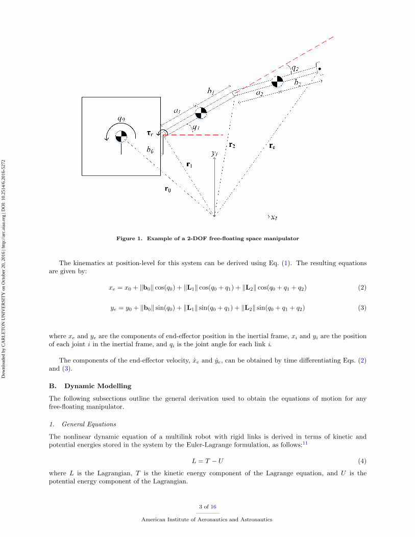
Figure 1. Example of a 2-DOF free-floating space manipulator

The kinematics at position-level for this system can be derived using Eq. (1). The resulting equationsare given by:

xe = x0 + ‖b0‖ cos(q0) + ‖L1‖ cos(q0 + q1) + ‖L2‖ cos(q0 + q1 + q2) (2)

ye = y0 + ‖b0‖ sin(q0) + ‖L1‖ sin(q0 + q1) + ‖L2‖ sin(q0 + q1 + q2) (3)

where xe and ye are the components of end-effector position in the inertial frame, xi and yi are the positionof each joint i in the inertial frame, and qi is the joint angle for each link i.

The components of the end-effector velocity, xe and ye, can be obtained by time differentiating Eqs. (2)and (3).

B. Dynamic Modelling

The following subsections outline the general derivation used to obtain the equations of motion for anyfree-floating manipulator.

1. General Equations

The nonlinear dynamic equation of a multilink robot with rigid links is derived in terms of kinetic andpotential energies stored in the system by the Euler-Lagrange formulation, as follows:11

L = T − U (4)

where L is the Lagrangian, T is the kinetic energy component of the Lagrange equation, and U is thepotential energy component of the Lagrangian.

3 of 16

American Institute of Aeronautics and Astronautics

Dow

nloa

ded

by C

AR

LE

TO

N U

NIV

ER

SIT

Y o

n O

ctob

er 2

0, 2

016

| http

://ar

c.ai

aa.o

rg |

DO

I: 1

0.25

14/6

.201

6-52

72

The kinetic and potential energies are defined in terms of generalized coordinates q ∈ Rn, whichencompass the position of the base satellite in inertial space as well as the joint angles. The equationsof motion for the two-link planar free-floating manipulator subjected to joint torques is derived according tothe following equation:

τi =d

dt

(∂L

∂qi

)−(∂L

∂qi

);∀i = 1, 2 (5)

where τi is the generalized joint torque for joint i. The kinetic energy is assumed to be a quadratic functionof the generalized coordinates q of the form:

T =1

2

n∑i=0

n∑j=0

Mij qiqj (6)

where Mij are the components of the robots inertia matrix, denoted M(q) ∈ Rn×n, which is symmetricand positive definite. In the case of a free-floating space manipulator with rigid links, there is no source ofpotential energy. Therefore, the Lagrangian can be simplified to:

L =1

2

n∑i=0

n∑j=0

Mij qiqj (7)

The partial derivative of the Lagrangian with respect to the kth joint position is given by:

∂L

∂qk=

1

2

n∑i=0

n∑j=0

∂Mij

∂qkqiqj (8)

Similarly, the partial derivative of the Lagrangian with respect to the kth joint velocity is given by:

∂L

∂qk=

n∑j=0

Mij qj (9)

Therefore, the derivative of Eq. (9) with respect to time is given by:

d

dt

(∂L

∂qk

)=

n∑j=0

Mij qj +

n∑i=0

n∑j=0

∂Mij

∂qiqiqj (10)

Thus, for each joint, the Euler-Lagrange equations are given by:

τk =

n∑j=0

Mij qj +

n∑i=0

n∑j=0

(∂Mij

∂qi− 1

2

∂Mij

∂qk

)qiqj (11)

It can be shown that:

n∑i=0

n∑j=0

(∂Mij

∂qi− 1

2

∂Mij

∂qk

)qiqj =

n∑i=0

n∑j=0

cijkqiqj (12)

where the terms cijk are known as the Christoffel symbols. The Euler-Lagrange equations of motion canthen be written as:

τk =

n∑j=0

Mij qj +

n∑i=0

n∑j=0

cijkqiqj (13)

where terms of the type q2i are called centrifugal, while those of the type qiqj are called the Coriolis terms.This expression can be rewritten once more into a more intuitive matrix form:

τ = M(q)q + C(q, q)q (14)

4 of 16

American Institute of Aeronautics and Astronautics

Dow

nloa

ded

by C

AR

LE

TO

N U

NIV

ER

SIT

Y o

n O

ctob

er 2

0, 2

016

| http

://ar

c.ai

aa.o

rg |

DO

I: 1

0.25

14/6

.201

6-52

72

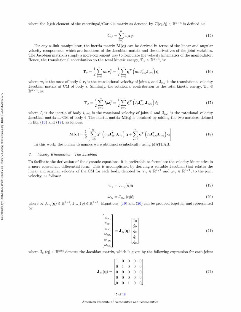
where the k,j th element of the centrifugal/Coriolis matrix as denoted by C(q, q) ∈ Rn×n is defined as:

Cij =

n∑i=1

cijkqi (15)

For any n-link manipulator, the inertia matrix M(q) can be derived in terms of the linear and angularvelocity components, which are functions of the Jacobian matrix and the derivatives of the joint variables.The Jacobian matrix is simply a more convenient way to formulate the velocity kinematics of the manipulator.Hence, the translational contribution to the total kinetic energy, Tv ∈ Rn×n, is:

Tv =1

2

n∑i=0

miv2i =

1

2

n∑i=0

qT(miJ

TcviJcvi

)q (16)

where mi is the mass of body i, vi is the translational velocity of joint i, and Jcvi is the translational velocityJacobian matrix at CM of body i. Similarly, the rotational contribution to the total kinetic energy, Tω ∈Rn×n, is:

Tω =1

2

n∑i=0

Iiω2i =

1

2

n∑i=0

qT(IiJ

Tcωi

Jcωi

)q (17)

where Ii is the inertia of body i, ωi is the rotational velocity of joint i, and Jcωiis the rotational velocity

Jacobian matrix at CM of body i. The inertia matrix M(q) is obtained by adding the two matrices definedin Eq. (16) and (17), as follows:

M(q) =1

2

[n∑i=0

qT(miJ

TcviJcvi

)q +

n∑i=0

qT(IiJ

Tcωi

Jcωi

)q

](18)

In this work, the planar dynamics were obtained symbolically using MATLAB.

2. Velocity Kinematics - The Jacobian

To facilitate the derivation of the dynamic equations, it is preferable to formulate the velocity kinematics ina more convenient differential form. This is accomplished by deriving a suitable Jacobian that relates thelinear and angular velocity of the CM for each body, denoted by vci ∈ R2×1 and ωci ∈ R3×1, to the jointvelocity, as follows:

vci = Jcvi(q)q (19)

ωci = Jcωi(q)q (20)

where by Jcvi(q) ∈ R2×5, Jcwi(q) ∈ R3×5. Equations (19) and (20) can be grouped together and representedby:

vcxi

vcyivcxi

ωcxi

ωcyiωczi

= Jci(q)

x0

y0

q0

q1

q2

(21)

where Jci(q) ∈ R5×5 denotes the Jacobian matrix, which is given by the following expression for each joint:

Jc0(q) =

1 0 0 0 0

0 1 0 0 0

0 0 0 0 0

0 0 0 0 0

0 0 1 0 0

(22)

5 of 16

American Institute of Aeronautics and Astronautics

Dow

nloa

ded

by C

AR

LE

TO

N U

NIV

ER

SIT

Y o

n O

ctob

er 2

0, 2

016

| http

://ar

c.ai

aa.o

rg |

DO

I: 1

0.25

14/6

.201

6-52

72

Jc1(q) =

1 0 −b0S0 − a1S1 −a1S1 0

0 1 b0C0 + a1C1 a1C1 0

0 0 0 0 0

0 0 0 0 0

0 0 1 1 0

(23)

Jc2(q) =

1 0 −b0S0 − L1S1 − a2S2 −L1S1 − a2S2 −a2S2

0 1 b0C0 + L1C1 + a2C2 L1C1 + a2C2 a2C2

0 0 0 0 0

0 0 0 0 0

0 0 1 1 1

(24)

where:S0 = sin(q0)S1 = sin(q0 + q1)S2 = sin(q0 + q1 + q2)C0 = cos(q0)C1 = cos(q0 + q1)C2 = cos(q0 + q1 + q2)L1 = a1 + b1

3. Derived Dynamic Equations for a 2-DOF Planar Manipulator

Using the Jacobian matrices defined in Eqs. (22) − (24), the translational contribution to the total kineticenergy can be written as:

Tv =1

2qT (m0J

Tcv0Jcv0 +m1J

Tcv1Jcv1 +m2J

Tcv2Jcv2)q (25)

Similarly, the rotational contribution to the total kinetic energy can be written as:

Tω =1

2qT (I0J

Tcω0

Jcω0+ I1J

Tcω1

Jcω1+ I2J

Tcω2

Jcω2)q (26)

As defined in Eq. (18), the inertia matrix M(q) is obtained by adding the two matrices in Eq. (25) and(26). The resulting matrix is the 5× 5 positive definite matrix as shown:

M(q) =

M11 M12 M13 M14 M15

M21 M22 M23 M24 M25

M31 M32 M33 M34 M35

M41 M42 M43 M44 M45

M51 M52 M53 M54 M55

(27)

where Mij ∀i = 1...5, j = 1...5 are defined in Appendix A. Using the components of the inertia matrix, theChristoffel symbols can be derived using Eq. (12). Then, from the Christoffel symbols with Eq. (15), theexpression for the 5× 5 centrifugal/Coriolis matrix can be derived:

C(q, q) =

C11 C12 C13 C14 C15

C21 C22 C23 C24 C25

C31 C32 C33 C34 C35

C41 C42 C43 C44 C45

C51 C52 C53 C54 C55

(28)

where Cij ∀i = 1...5, j = 1...5 are also defined in Appendix A.

6 of 16

American Institute of Aeronautics and Astronautics

Dow

nloa

ded

by C

AR

LE

TO

N U

NIV

ER

SIT

Y o

n O

ctob

er 2

0, 2

016

| http

://ar

c.ai

aa.o

rg |

DO

I: 1

0.25

14/6

.201

6-52

72

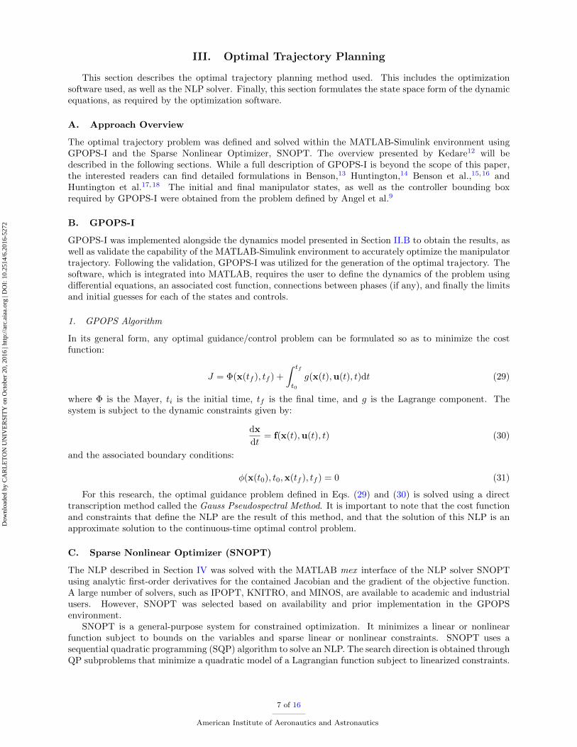
III. Optimal Trajectory Planning

This section describes the optimal trajectory planning method used. This includes the optimizationsoftware used, as well as the NLP solver. Finally, this section formulates the state space form of the dynamicequations, as required by the optimization software.

A. Approach Overview

The optimal trajectory problem was defined and solved within the MATLAB-Simulink environment usingGPOPS-I and the Sparse Nonlinear Optimizer, SNOPT. The overview presented by Kedare12 will bedescribed in the following sections. While a full description of GPOPS-I is beyond the scope of this paper,the interested readers can find detailed formulations in Benson,13 Huntington,14 Benson et al.,15,16 andHuntington et al.17,18 The initial and final manipulator states, as well as the controller bounding boxrequired by GPOPS-I were obtained from the problem defined by Angel et al.9

B. GPOPS-I

GPOPS-I was implemented alongside the dynamics model presented in Section II.B to obtain the results, aswell as validate the capability of the MATLAB-Simulink environment to accurately optimize the manipulatortrajectory. Following the validation, GPOPS-I was utilized for the generation of the optimal trajectory. Thesoftware, which is integrated into MATLAB, requires the user to define the dynamics of the problem usingdifferential equations, an associated cost function, connections between phases (if any), and finally the limitsand initial guesses for each of the states and controls.

1. GPOPS Algorithm

In its general form, any optimal guidance/control problem can be formulated so as to minimize the costfunction:

J = Φ(x(tf ), tf ) +

∫ tf

t0

g(x(t),u(t), t)dt (29)

where Φ is the Mayer, ti is the initial time, tf is the final time, and g is the Lagrange component. Thesystem is subject to the dynamic constraints given by:

dx

dt= f(x(t),u(t), t) (30)

and the associated boundary conditions:

φ(x(t0), t0,x(tf ), tf ) = 0 (31)

For this research, the optimal guidance problem defined in Eqs. (29) and (30) is solved using a directtranscription method called the Gauss Pseudospectral Method. It is important to note that the cost functionand constraints that define the NLP are the result of this method, and that the solution of this NLP is anapproximate solution to the continuous-time optimal control problem.

C. Sparse Nonlinear Optimizer (SNOPT)

The NLP described in Section IV was solved with the MATLAB mex interface of the NLP solver SNOPTusing analytic first-order derivatives for the contained Jacobian and the gradient of the objective function.A large number of solvers, such as IPOPT, KNITRO, and MINOS, are available to academic and industrialusers. However, SNOPT was selected based on availability and prior implementation in the GPOPSenvironment.

SNOPT is a general-purpose system for constrained optimization. It minimizes a linear or nonlinearfunction subject to bounds on the variables and sparse linear or nonlinear constraints. SNOPT uses asequential quadratic programming (SQP) algorithm to solve an NLP. The search direction is obtained throughQP subproblems that minimize a quadratic model of a Lagrangian function subject to linearized constraints.

7 of 16

American Institute of Aeronautics and Astronautics

Dow

nloa

ded

by C

AR

LE

TO

N U

NIV

ER

SIT

Y o

n O

ctob

er 2

0, 2

016

| http

://ar

c.ai

aa.o

rg |

DO

I: 1

0.25

14/6

.201

6-52

72

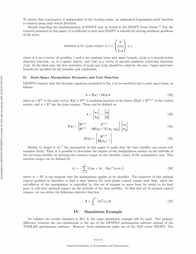
To ensure that convergence is independent of the starting point, an augmented Lagrangian merit functionis reduced along each search direction.

Details regarding the implementation of SNOPT may be found in the SNOPT Users Guide.19 For theresearch presented in this paper, it is sufficient to note that SNOPT is suitable for solving nonlinear problemsof the form:

minimize x for f0(x) subject to l ≤

x

f(x)

ALx

≤ uwhere x is an n-vector of variables, l and u are constant lower and upper bounds, f0(x) is a smooth scalarobjective function, AL is a sparse matrix, and f(x) is a vector of smooth nonlinear constraint functionsfi(x). In the ideal case, the first derivative of f0(x) and fi(x) should be coded by the user. Upper and lowerbounds are specified for all variables and constraints.

D. State-Space Manipulator Dynamics and Cost Function

GPOPS-I requires that the dynamic equations presented in Eq. (14) be rewritten into a state space-form, asfollows:

x = f(x) + G(x)τ (32)

where x ∈ R2n is the state vector; f(x) ∈ R2n is nonlinear function of the states; G(x) ∈ R2n×n is the controlmatrix; and τ ∈ Rn are the joint torques. These can be defined as:

x =

[x1

x2

]=

[q

q

](33)

f(x) =

[05×5 15×5

05×5 −M(x1)−1C(x1,x2)

][x1

x2

](34)

G(x) =

[05×5

M(x1)−1

](35)

Similar to Angel et al.,9 the assumption in this paper is made that the base satellite can rotate andtranslate freely. Thus, it is possible to determine the impact of the manipulators motion on the attitude ofthe servicing satellite by deriving the reaction torque on the shoulder (base) of the manipulator arm. Thisreaction torque can be defined by:

τr = −n∑i=1

(Iiαi + (ri − b0)×(mivi)) (36)

where τr ∈ Rn is the moment that the manipulator applies at its shoulder. The objective of this optimalcontrol problem is therefore to find a time history for each joints control torque such that, when theend-effector of the manipulator is controlled by this set of torques to move from its initial to its finalpose, it will have minimal impact on the attitude of the base satellite. To find this set of optimal controltorques, we can define the following objective function:

J =

∫ tf

0

(τTr τr

)dt (37)

IV. Simulation Example

To validate the results obtained in Ref. 9, the same simulation example will be used. The primarydifference between the two simulations is the use of the GPOPS-I optimization software instead of theTOMLAB optimization software. However, both simulations make use of the NLP solver SNOPT. The

8 of 16

American Institute of Aeronautics and Astronautics

Dow

nloa

ded

by C

AR

LE

TO

N U

NIV

ER

SIT

Y o

n O

ctob

er 2

0, 2

016

| http

://ar

c.ai

aa.o

rg |

DO

I: 1

0.25

14/6

.201

6-52

72

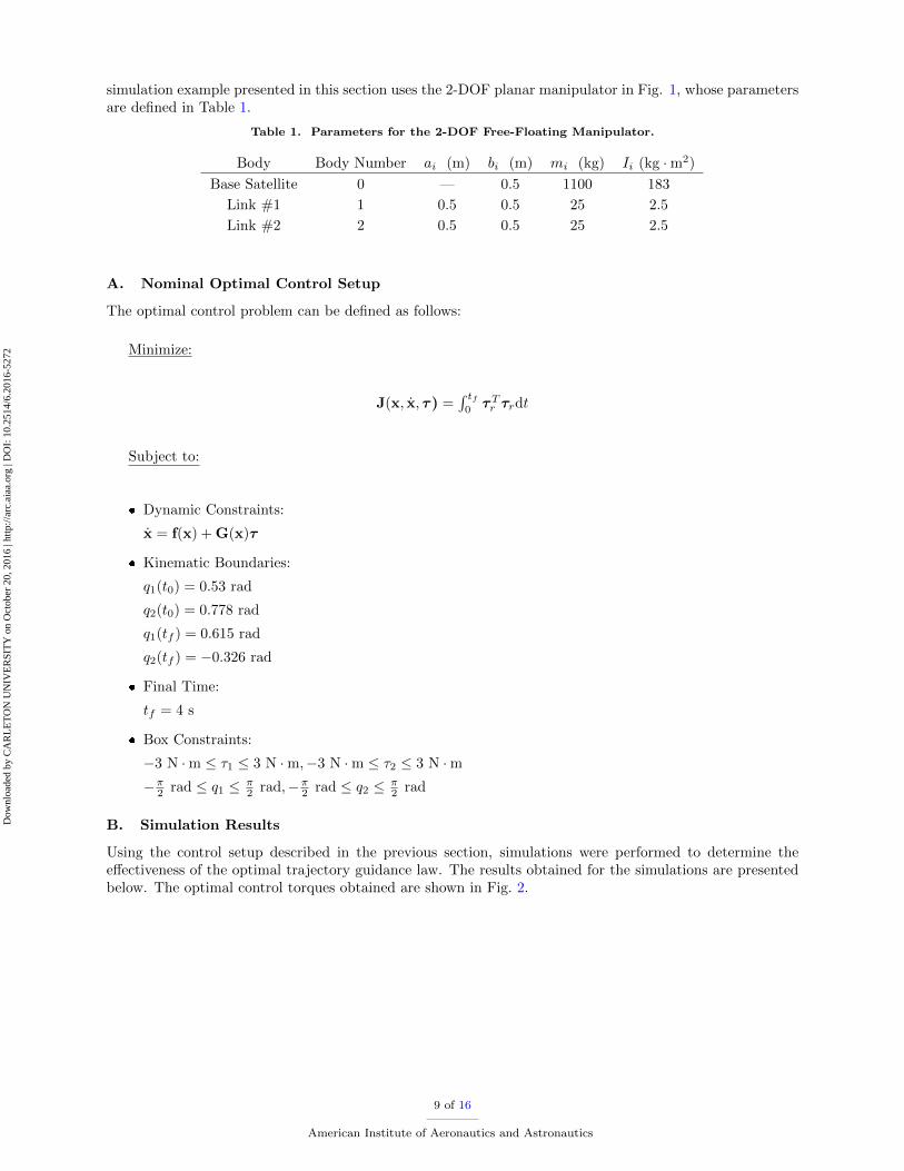
simulation example presented in this section uses the 2-DOF planar manipulator in Fig. 1, whose parametersare defined in Table 1.

Table 1. Parameters for the 2-DOF Free-Floating Manipulator.

Body Body Number ai (m) bi (m) mi (kg) Ii (kg ·m2)

Base Satellite 0 — 0.5 1100 183

Link #1 1 0.5 0.5 25 2.5

Link #2 2 0.5 0.5 25 2.5

A. Nominal Optimal Control Setup

The optimal control problem can be defined as follows:

Minimize:

J(x, x, τ ) =∫ tf0τTr τrdt

Subject to:

� Dynamic Constraints:

x = f(x) + G(x)τ

� Kinematic Boundaries:

q1(t0) = 0.53 rad

q2(t0) = 0.778 rad

q1(tf ) = 0.615 rad

q2(tf ) = −0.326 rad

� Final Time:

tf = 4 s

� Box Constraints:

−3 N ·m ≤ τ1 ≤ 3 N ·m,−3 N ·m ≤ τ2 ≤ 3 N ·m−π2 rad ≤ q1 ≤ π

2 rad,−π2 rad ≤ q2 ≤ π2 rad

B. Simulation Results

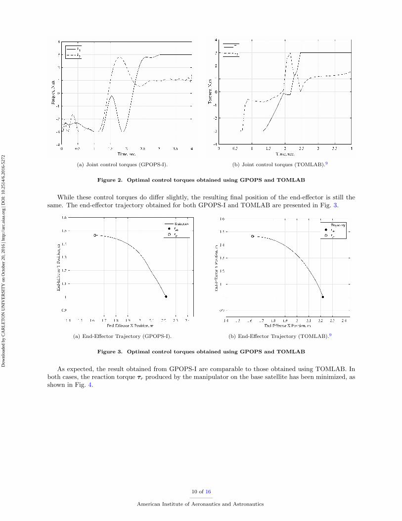
Using the control setup described in the previous section, simulations were performed to determine theeffectiveness of the optimal trajectory guidance law. The results obtained for the simulations are presentedbelow. The optimal control torques obtained are shown in Fig. 2.

9 of 16

American Institute of Aeronautics and Astronautics

Dow

nloa

ded

by C

AR

LE

TO

N U

NIV

ER

SIT

Y o

n O

ctob

er 2

0, 2

016

| http

://ar

c.ai

aa.o

rg |

DO

I: 1

0.25

14/6

.201

6-52

72

(a) Joint control torques (GPOPS-I). (b) Joint control torques (TOMLAB).9

Figure 2. Optimal control torques obtained using GPOPS and TOMLAB

While these control torques do differ slightly, the resulting final position of the end-effector is still thesame. The end-effector trajectory obtained for both GPOPS-I and TOMLAB are presented in Fig. 3.

(a) End-Effector Trajectory (GPOPS-I). (b) End-Effector Trajectory (TOMLAB).9

Figure 3. Optimal control torques obtained using GPOPS and TOMLAB

As expected, the result obtained from GPOPS-I are comparable to those obtained using TOMLAB. Inboth cases, the reaction torque τr produced by the manipulator on the base satellite has been minimized, asshown in Fig. 4.

10 of 16

American Institute of Aeronautics and Astronautics

Dow

nloa

ded

by C

AR

LE

TO

N U

NIV

ER

SIT

Y o

n O

ctob

er 2

0, 2

016

| http

://ar

c.ai

aa.o

rg |

DO

I: 1

0.25

14/6

.201

6-52

72

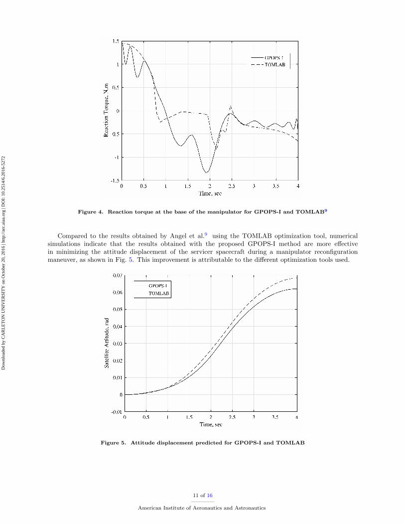
Figure 4. Reaction torque at the base of the manipulator for GPOPS-I and TOMLAB9

Compared to the results obtained by Angel et al.9 using the TOMLAB optimization tool, numericalsimulations indicate that the results obtained with the proposed GPOPS-I method are more effectivein minimizing the attitude displacement of the servicer spacecraft during a manipulator reconfigurationmaneuver, as shown in Fig. 5. This improvement is attributable to the different optimization tools used.

Figure 5. Attitude displacement predicted for GPOPS-I and TOMLAB

11 of 16

American Institute of Aeronautics and Astronautics

Dow

nloa

ded

by C

AR

LE

TO

N U

NIV

ER

SIT

Y o

n O

ctob

er 2

0, 2

016

| http

://ar

c.ai

aa.o

rg |

DO

I: 1

0.25

14/6

.201

6-52

72

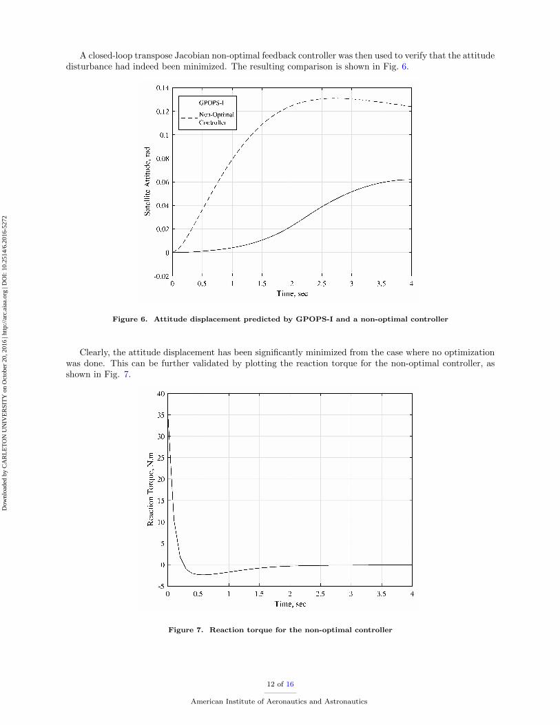
A closed-loop transpose Jacobian non-optimal feedback controller was then used to verify that the attitudedisturbance had indeed been minimized. The resulting comparison is shown in Fig. 6.

Figure 6. Attitude displacement predicted by GPOPS-I and a non-optimal controller

Clearly, the attitude displacement has been significantly minimized from the case where no optimizationwas done. This can be further validated by plotting the reaction torque for the non-optimal controller, asshown in Fig. 7.

Figure 7. Reaction torque for the non-optimal controller

12 of 16

American Institute of Aeronautics and Astronautics

Dow

nloa

ded

by C

AR

LE

TO

N U

NIV

ER

SIT

Y o

n O

ctob

er 2

0, 2

016

| http

://ar

c.ai

aa.o

rg |

DO

I: 1

0.25

14/6

.201

6-52

72

The reaction torque for the non-optimal case is significantly larger then it was for the optimized case. Thisindicates that the technique validated in this paper is very effective at reducing the attitude displacementresulting from the motion of the manipulator.

V. Conclusion

In this paper, a nonlinear optimal guidance law for free-floating manipulators was validated. This wasaccomplished by first deriving the kinematic and dynamic equations for a planar free-floating manipulator,which described the motion of the end-effector as a function of the generalized joint coordinates. Next, theoptimal trajectory planning technique was presented and a cost function was defined. Finally, a dynamicsimulation for a 2-DOF free-floating manipulator was used to demonstrate the performance of the technique,and the results compared favourably to past research. Ultimately, this paper demonstrated that the nonlinearoptimal guidance law is more effective at minimizing the attitude disturbance of a base satellite, comparedto an existing optimal guidance law and to a non-optimal transpose Jacobian control law. Future work willinclude the experimental validations of the proposed optimization scheme.

13 of 16

American Institute of Aeronautics and Astronautics

Dow

nloa

ded

by C

AR

LE

TO

N U

NIV

ER

SIT

Y o

n O

ctob

er 2

0, 2

016

| http

://ar

c.ai

aa.o

rg |

DO

I: 1

0.25

14/6

.201

6-52

72

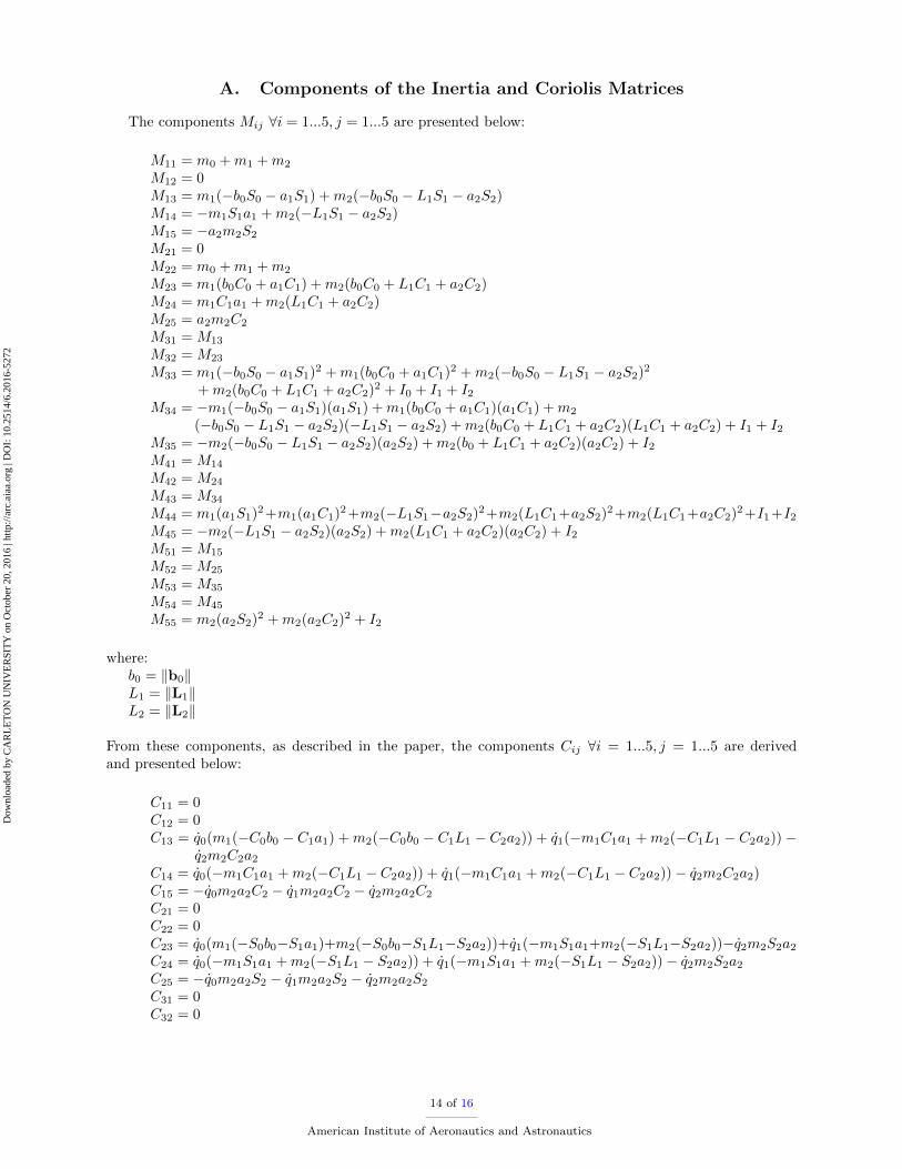
A. Components of the Inertia and Coriolis Matrices

The components Mij ∀i = 1...5, j = 1...5 are presented below:

M11 = m0 +m1 +m2

M12 = 0M13 = m1(−b0S0 − a1S1) +m2(−b0S0 − L1S1 − a2S2)M14 = −m1S1a1 +m2(−L1S1 − a2S2)M15 = −a2m2S2

M21 = 0M22 = m0 +m1 +m2

M23 = m1(b0C0 + a1C1) +m2(b0C0 + L1C1 + a2C2)M24 = m1C1a1 +m2(L1C1 + a2C2)M25 = a2m2C2

M31 = M13

M32 = M23

M33 = m1(−b0S0 − a1S1)2 +m1(b0C0 + a1C1)2 +m2(−b0S0 − L1S1 − a2S2)2

+m2(b0C0 + L1C1 + a2C2)2 + I0 + I1 + I2M34 = −m1(−b0S0 − a1S1)(a1S1) +m1(b0C0 + a1C1)(a1C1) +m2

(−b0S0 − L1S1 − a2S2)(−L1S1 − a2S2) +m2(b0C0 + L1C1 + a2C2)(L1C1 + a2C2) + I1 + I2M35 = −m2(−b0S0 − L1S1 − a2S2)(a2S2) +m2(b0 + L1C1 + a2C2)(a2C2) + I2M41 = M14

M42 = M24

M43 = M34

M44 = m1(a1S1)2+m1(a1C1)2+m2(−L1S1−a2S2)2+m2(L1C1+a2S2)2+m2(L1C1+a2C2)2+I1+I2M45 = −m2(−L1S1 − a2S2)(a2S2) +m2(L1C1 + a2C2)(a2C2) + I2M51 = M15

M52 = M25

M53 = M35

M54 = M45

M55 = m2(a2S2)2 +m2(a2C2)2 + I2

where:b0 = ‖b0‖L1 = ‖L1‖L2 = ‖L2‖

From these components, as described in the paper, the components Cij ∀i = 1...5, j = 1...5 are derivedand presented below:

C11 = 0C12 = 0C13 = q0(m1(−C0b0 − C1a1) +m2(−C0b0 − C1L1 − C2a2)) + q1(−m1C1a1 +m2(−C1L1 − C2a2))−

q2m2C2a2C14 = q0(−m1C1a1 +m2(−C1L1 − C2a2)) + q1(−m1C1a1 +m2(−C1L1 − C2a2))− q2m2C2a2)C15 = −q0m2a2C2 − q1m2a2C2 − q2m2a2C2

C21 = 0C22 = 0C23 = q0(m1(−S0b0−S1a1)+m2(−S0b0−S1L1−S2a2))+q1(−m1S1a1+m2(−S1L1−S2a2))−q2m2S2a2C24 = q0(−m1S1a1 +m2(−S1L1 − S2a2)) + q1(−m1S1a1 +m2(−S1L1 − S2a2))− q2m2S2a2C25 = −q0m2a2S2 − q1m2a2S2 − q2m2a2S2

C31 = 0C32 = 0

14 of 16

American Institute of Aeronautics and Astronautics

Dow

nloa

ded

by C

AR

LE

TO

N U

NIV

ER

SIT

Y o

n O

ctob

er 2

0, 2

016

| http

://ar

c.ai

aa.o

rg |

DO

I: 1

0.25

14/6

.201

6-52

72

C33 = q0(m1(−S0b0 − S1a1)(−C0b0 − C1a1) +m1(C0b0 + C1a1)(−S0b0 − S1a1) +m2(−S0b0−S1L1−S2a2)(−C0b0−C1L1−C2a2)+m2(C0b0+C1L1+C2a2)(−S0b0−S1L1−S2a2))+q1(−m1(−S0b0−S1a1)C1a1−m1(C0b0+C1a1)S1a1+m2(−S0b0−S1L1−S2a2)(−C1L1−C2a2)+m2(C0b0 + C1L1 + C2a2)(−S1L1 − S2a2)) + q2(−m2(−S0b0 − S1L1 − S2a2)C2a2−m2(C0b0 + C1L1 + C2a2)S2a2)

C34 = q0(−m1(−S0b0 − S1a1)C1a1 −m1(C0b0 + C1a1)S1a1+m2(−S0b0 − S1L1 − S2a2)(−S0b0 − S1a1) +m2(C0b0 + C1L1 + C2a2)(−S1L1 − S2a2)) + q1(−m1(−S0b0 − S1a1)C1a1 −m1(C0b0 + C1a1)S1a1+m2(−S0b0 − S1L1 − S2a2)(−C1L1 − C2a2) +m2(C0b0 + C1L1 + C2a2)(−S1L1 − S2a2)) + q2(−m2(−S0b0 − S1L1 − S2a2)C2a2 −m2(C0b0 + C1L1 + C2a2)S2a2)

C35 = q0(−m2(−S0b0 − S1L1 − S2a2)C2a2 −m2(C0b0 + C1L1 + C2a2)S2a2)+ q1(−m2(−S0b0 − S1L1 − S2a2)C2a2 −m2(C0b0 + C1L1 + C2a2)S2a2)+ q2(−m2(−S0b0 − S1L1 − S2a2)C2a2 −m2(C0b0 + C1L1 + C2a2)S2a2)

C41 = 0C42 = 0C43 = q0(−m1(−C0b0 − C1a1)S1a1 +m2(−C0b0 − C1L1 − C2a2)(−S1L1 − S2a2)

+m2(−S0b0 − S1L1 − S2a2)(C1L1 + C2a2) +m1(−S0b0 − S1a1)C1a1)+ q1(m2(−C1L1 − C2a2)(−S1L1 − S2a2) +m2(−S1L1 − S2a2)(C1L1 + C2a2))+ q2(−m2S2a2(C1L1 + C2a2)−m2(−S1L1 − S2a2)C2a2)

C44 = q0(m2(−C1L1 − C2a2)(−S1L1 − S2a2) +m2(−S1L1 − S2a2)(C1L1 + C2a2))+ q1(m2(−C1L1 − C2a2)(−S1L1 − S2a2) +m2(−S1L1 − S2a2)(C1L1 + C2a2))+ q2(−m2S2a2(C1L1 + C2a2)−m2(−S1L1 − S2a2)C2a2)

C45 = q0(−m2S2a2(C1L1 + C2a2)−m2(−S1L1 − S2a2)C2a2)+ q1(−m2S2a2(C1L1 + C2a2)−m2(−S1L1 − S2a2)C2a2)+ q2(−m2S2a2(C1L1 + C2a2)−m2(−S1L1 − S2a2)C2a2)

C51 = 0C52 = 0C53 = q0(−m2(−C0b0 − C1L1 − C2a2)S2a2 +m2(−S0b0 − S1L1 − S2a2)C2a2)

+ q1(−m2(−C1L1 − C2a2)S2a2 +m2(−S1L1 − S2a2)C2a2)C54 = q0(−m2(−C1L1 − C2a2)S2a2 +m2(−S1L1 − S2a2)C2a2)

+ q1(−m2(−C1L1 − C2a2)S2a2 +m2(−S1L1 − S2a2)C2a2)C55 = 0

15 of 16

American Institute of Aeronautics and Astronautics

Dow

nloa

ded

by C

AR

LE

TO

N U

NIV

ER

SIT

Y o

n O

ctob

er 2

0, 2

016

| http

://ar

c.ai

aa.o

rg |

DO

I: 1

0.25

14/6

.201

6-52

72

Acknowledgments

The authors would like to express their sincere gratitude to Angel Flores-Abad from the New MexicoState University for providing the raw data that helped us benchmark the new results obtained in this work.

References

1Kessler, D. J., Johnson, N. L., Liou, J.-C., and Matney, M., “The Kessler Syndrome: Implications to Future SpaceOperations,” in 33rd Annual AAS Guidance and Control Conference, San Diego, CA, 2010, Feb. 6–10.2“Enabling Large-Body Active Debris Removal Project.” Space Technology Mission Directorate (STMD), NASA, TX,

United States, 2015.3Dubowsky, S. and Torres, M., “Path Planning for Space Manipulators to Minimize Spacecraft Attitude Disturbances,” in

IEEE International Conference on Robotics and Automation, Sacramento, CA., 1991, pp. 2522-2528.4Agrawal, O. P. and Xu, Y., “On the global optimum path planning for redundant space manipulators,” in IEEE

Transactions on Man and Cybernetics, 1994, pp. 1306–1316.5Papadopoulos, E. Abu-Abed, A., “Design and Motion Planning for a Zero-Reaction Manipulator,” in IEEE International

Conference on Robotics and Automation, San Diego, CA., 1994, pp. 1554–1559.6Lampariello, R., Agrawal, S. and Hirzinger, H., “Optimal Motion Planning for Free-Flying Robots,” in IEEE International

Conference on Robotics and Automation, Taipei, Taiwan., 2003, pp. 3029-3035.7Aghili, F., “Optimal Control for Robotic Capturing and Passivation of a Tumbling Satellite with Unknown Dynamics” in

AIAA Guidance Navigation and Control Conference, Honolulu, Hawaii, 2008, pp. 1–21.8Oki, T. Nakanishi, H and Yoshida, K., “Time-Optimal Manipulator Control of a Free-Floating Space Robot with Constraint

on Reaction Torque” in IEEE International Conference on Intelligent Robots and Systems, Nice, France, 2008, pp. 2828-2833.9Flores-Abad, A. Wei, A. Ma, O. Pham, K., “Optimal Control of Space Robots for Capturing a Tumbling Object with

Uncertainties,” Journal of Guidance, Control, and Dynamics, vol. 37, no. 6, 2014, pp. 2014-2017.10Yoshida, K. and Umetani, Y., Space Robotics: Dynamics and Control. Tokyo: Kluwer Academic Publishers, 1993.11Ulrich, S., ”Direct Adaptive Control Methodologies for Flexible-Joint Space Manipulators with Uncertainties and ModellingErrors.” Ph.D. thesis, Department of Mechanical and Aerospace Engineering, Carleton University, Ottawa, Canada, 2012.12Kedare, S., ”Space Environment Modelling and Torque-Optimal Guidance for CubeSat Applications.” M.A.Sc. thesis,Department of Mechanical and Aerospace Engineering, Carleton University, Ottawa, Canada, 2014.13Benson, D. A., ”A Gauss Pseudospectral Transcription for Optimal Control”, Ph.D. Thesis, Dept of Aeronautics andAstronautics, MIT, November 2004.14Huntington, G. T., ”Advancements and Analysis of Gauss Pseudospectral Transcription for Optimal Control”, Ph.D.Thesis, Dept of Aeronautics and Astronautics, MIT, May 2007.15Benson, D. A., Huntington, G. T., Thorvaldsen, T. P., and Rao, A. V., “Direct Trajectory Optmization and CostateEstimation via an Orthagonal Collocation Method,” Journal of Guidance, Control, and Dynamics, vol. 29, no. 6, 2006, pp.1435–1440.16Benson, D. A., Huntington, G. T., and Rao, A. V., “Design of Optimal Tetrahedral Spacecraft Formations,” Journal ofAstronautical Sciences, vol. 55, no. 2, 2007, pp. 141–169.17Huntington, G. T., Benson, D. A., How, J. P., Kanizay, N., Darby, C. L., and Rao, A. V., “Computation of BoundaryControls Using a Gauss Pseudospectral Method,” in 2007 Astrodynamics Specialist Conference, Mackinac Island, Michigan,August 2007.18Huntington, G. T., and Rao, A. V., “Optimal Reconfiguration of Spacecraft Formations Using a Gauss PseudospectralMethod,” Journal of Guidance, Control, and Dynamics, vol. 31, no. 3, 2008, pp. 689–698.19Gill, P. E. Murray, W. and Saunders, M. A., User Guide for SNOPT Version 7: Software for Large-Scale NonlinearProgramming, June 2008.20Espero, M. T., “Future Space Robotics and Large Optical Systems: A Picture of Orbital Express,” Ares V Workshop,California, USA, 2008.

16 of 16

American Institute of Aeronautics and Astronautics

Dow

nloa

ded

by C

AR

LE

TO

N U

NIV

ER

SIT

Y o

n O

ctob

er 2

0, 2

016

| http

://ar

c.ai

aa.o

rg |

DO

I: 1

0.25

14/6

.201

6-52

72