Optimal Automatic Stabilizers∗

Alisdair McKay

Boston University

Ricardo Reis

London School of Economics

October 2017

Abstract

Should the generosity of unemployment benefits and the progressivity of income taxes de-

pend on the presence of business cycles? This paper proposes a tractable model where there is

a role for social insurance against uninsurable shocks to income and unemployment, as well as

inefficient business cycles driven by aggregate shocks through matching frictions and nominal

rigidities. We derive an augmented Baily-Chetty formula showing that the optimal generosity

and progressivity depend on a macroeconomic stabilization term. This term pushes for an in-

crease in generosity and progressivity when the level of economic activity is more responsive

to social programs in recessions than in booms. A calibration to the U.S. economy shows that

taking concerns for macroeconomic stabilization into account raises the optimal unemployment

insurance replacement rate by 20 percentage points but has a negligible impact on the optimal

progressivity of the income tax. More generally, the role of social insurance programs as auto-

matic stabilizers affects their optimal design.

JEL codes: E62, H21, H30.

Keywords: Counter-cyclical fiscal policy; Redistribution; Distortionary taxes.

∗Contact: amckay@bu.edu and r.a.reis@lse.ac.uk. First draft: February 2015. We are grateful to Ralph Luetticke,Pascal Michaillat, Vincent Sterk, for insightful discussions, and to many seminar participants for useful comments.

1 Introduction

The usual motivation behind large social welfare programs, like unemployment insurance or pro-

gressive income taxation, is to provide social insurance and engage in redistribution. An extensive

literature therefore studies the optimal progressivity of income taxes typically by weighing the dis-

incentive effect on individual labor supply and savings against concerns for redistribution and for

insurance against idiosyncratic income shocks.1 In turn, the optimal generosity of unemployment

benefits is often stated in terms of a Baily-Chetty formula, which weighs the moral hazard effect

of unemployment insurance on job search and creation against the social insurance benefits that it

provides.2

For the most part, this literature abstracts from aggregate shocks, so that the optimal generosity

and progressivity do not take into account business cycles. Yet, from their inception, an auxiliary

justification for these social programs was that they were also supposed to automatically stabilize

the business cycle.3 The classic work that focussed on the automatic stabilizers relied on a Keyne-

sian tradition that ignored the social insurance that these programs provide or their disincentive

effects on employment. Some recent work brings these two orthogonal literatures together, but so

far it has focused on the positive effects of the automatic stabilizers, falling short of computing

optimal policies.4

The goal of this paper is to answer two classic questions—How generous should unemployment

benefits be? How progressive should income taxes be?—but taking into account their automatic

stabilizer benefits as well as their social insurance benefits. We present a model in which there

is both a role for social insurance as well as aggregate shocks and inefficient business cycles. We

introduce unemployment insurance and progressive income taxes as automatic stabilizers, that is,

programs that do not directly depend on the aggregate state of the economy even if the aggregate

size of the programs changes with the composition of income in the economy. We then solve for the

ex ante socially optimal replacement rate of unemployment benefits and progressivity of personal

income taxes in the presence of uninsured income risks, precautionary savings motives, labor market

1Mirrlees (1971) and Varian (1980) are classic references, and more recently see Benabou (2002), Conesa andKrueger (2006), Heathcote et al. (2014), Krueger and Ludwig (2013), and Golosov et al. (2016).

2See the classic work by Baily (1978) and Chetty (2006).3Musgrave and Miller (1948) and Auerbach and Feenberg (2000) are classic references, while Blanchard et al.

(2010) is a recent call for more modern work in this topic.4See McKay and Reis (2016) for a recent model, DiMaggio and Kermani (2016) for recent empirical work, and

IMF (2015) for the shortcomings of the older literature.

1

frictions, and nominal rigidities.

Our first main contribution is to provide a formal, theory-grounded definition of an automatic

stabilizer. We show that a business-cycle variant of the Baily-Chetty formula for unemployment

insurance and a similar formula for the optimal choice of progressivity of the tax system are both

augmented by a new macroeconomic stabilization term. This term equals the expectation of the

product of the welfare gain from eliminating economic slack with the elasticity of slack with respect

to the replacement rate or tax progressivity. Even if the economy is efficient on average, economic

fluctuations may lead to more generous unemployment insurance or more progressive income taxes,

relative to standard analyses that ignore the automatic stabilizer properties of these programs.

This term captures the automatic stabilizer nature of social insurance programs.

The second contribution is to characterize this macroeconomic stabilization term analytically to

understand the different economic mechanisms behind it. Fluctuations in aggregate economic slack,

measured by the unemployment rate, the output gap or the job finding rate, can lead to welfare

losses through four separate channels. First, they may create a wedge between the marginal disu-

tility of hours worked and the social benefit of work. This inefficiency appears in standard models

of inefficient business cycles, and is sometimes described as a result of time-varying markups (Chari

et al., 2007; Galı et al., 2007). Second, when labor markets are tight, more workers are employed

raising production but the cost of recruiting and hiring workers rises. The equilibrium level of un-

employment need not be efficient as hiring and search decisions do not necessarily internalize these

tradeoffs. This is the source of inefficiency common to search models (e.g. Hosios, 1990). Third,

the state of the business cycle alters the extent of uninsurable risk that households face both in

unemployment and income risk. This is the source of welfare costs of business cycles that has

been studied by Storesletten et al. (2001), Krebs (2003, 2007), and De Santis (2007). Finally, with

nominal rigidities, slack affects inflation and the dispersion of relative prices, as emphasized by the

new Keynesian business cycle literature (Woodford, 2010; Gali, 2011). Our measure isolates these

four effects cleanly in terms of separate additive terms in the condition determining the optimal

extent of the social insurance programs.

As for the elasticity of slack with respect to social programs, unemployment benefits and pro-

gressive taxes can stabilize the economy even if these policies are themselves not responsive to the

business cycle. For one, these policies redistribute across groups who may have different marginal

2

propensities to consume. In the case of unemployment insurance, the magnitude of this redistri-

bution increases when more people become unemployed in a recession. Moreover, these policies

mitigate precautionary savings motives by providing social insurance. Because the risk in pre-tax

incomes rises in a recession, the effect of this social insurance on aggregate demand rises as well, so

these policies stabilize aggregate demand. We further show that if prices are flexible so aggregate

demand matters little, or if monetary policy aggressively stabilizes the business cycle, then little

role is left for the social programs to work as stabilizers.

Our third contribution is to investigate the magnitude of the macroeconomic stabilization term

and the key mechanisms behind it. We calculate the optimal unemployment replacement rate and

tax progressivity and compare these values to what one would find in the absence of aggregate risk.

We find a large effect on unemployment insurance: with business cycles, the optimal unemployment

replacement rate rises from 41 to 61 percent. However, the level of tax progressivity has little

stabilizing effect on the business cycle so the presence of aggregate shocks has almost no effect on

the optimal degree of progressivity.

Our analytical results allow us to interpret these numerical results, by allowing us to quantify

the tradeoffs between incentives, social insurance and macroeconomic stabilization and the con-

stituent mechanisms of the macroeconomic stabilization term. This highlights the usefulness of the

propositions, which are expressed in general terms and involving aggregate endogenous variables,

so that they can be used in different models and circumstances while isolating the key forces at

hand. Quantitatively, the automatic stabilizer term is large in the case of unemployment benefits,

and largely driven by the effect of the business cycle on the extent of uninsurable idiosyncratic risk.

Finally, we use a numerical analysis of the model as a laboratory to explore the roles of some

assumptions that we made for analytical tractability. Namely, our baseline results rely on a de-

generate wealth distribution for tractability, but we show that allowing for heterogeneity in wealth

does not much alter the relative strengths of the tradeoffs so our conclusion about the importance

of the macroeconomic stabilization term for the optimal policy is relatively robust.

There are large literatures on the three topics that we touch on: business cycle models with

incomplete markets and nominal rigidities, social insurance and public programs, and automatic

stabilizers. Our model of aggregate demand has some of the key features of new Keynesian models

with labor markets (Gali, 2011) but that literature focuses on optimal monetary policy, whereas we

3

study the optimal design of the social insurance system. Our model of incomplete markets builds on

McKay and Reis (2016), Ravn and Sterk (2017), and Heathcote et al. (2014) to generate a tractable

model of incomplete markets and automatic stabilizers. This simplicity allows us to analytically

express optimality conditions for generosity and progressivity, and to, even in a more general case,

easily solve the model numerically and so be able to search for the optimal policies. Finally, our

paper is part of a surge of work on the interplay of nominal rigidities and precautionary savings,

but this literature has mostly been positive whereas this paper’s focus is on optimal policy.5

On the generosity of unemployment insurance, our work is closest to Landais et al. (2017) and

Kekre (2017). They also couch their analysis in terms of the standard Baily-Chetty formula by

considering the general equilibrium effects of unemployment insurance. The main difference is that

they study benefits as discretionary policy instruments that vary over the business cycle, while we

study how the presence of business cycles affects the ex ante fixed level of benefits.6 Our focus is

on automatic stabilizers, an ex ante passive policy, while they consider active stabilization policy,

which are quite different questions as the long literature on rules versus discretion in macroeco-

nomics attests.7 Moreover, our model includes aggregate uncertainty, and we also study income

tax progressivity.

On income taxes, our work is closest to Benabou (2002) and Bhandari et al. (2017). Our

dynamic heterogeneous-agent model with progressive income taxes is similar to the one in Benabou

(2002), but our focus is on business cycles, so we complement it with aggregate shocks and nominal

rigidities. Bhandari et al. (2017) is one of the very few studies of optimal income taxes with

aggregate shocks. Like us, those authors emphasize the interaction between business cycles and the

desire for redistribution.8 However, they solve for the Ramsey optimal fiscal policy, which adjusts

the tax instruments every period in response to shocks, while we choose the ex ante optimal rules

for generosity and progressivity. This is consistent with our focus on automatic stabilizers, which

are ex ante fiscal systems, rather than counter-cyclical policies.

Finally, this paper is related to the modern study of automatic stabilizers and especially our

5See Oh and Reis (2012); Guerrieri and Lorenzoni (2011); Auclert (2016); McKay et al. (2016); Kaplan et al.(2016); Werning (2015).

6See also Mitman and Rabinovich (2011), Jung and Kuester (2015), and Den Haan et al. (2015).7Unlike the United States, where the duration of unemployment benefits is often increased during recessions, in

most OECD countries the terms of unemployment insurance programs do not change over the business cycle, asdescribed in http://www.oecd.org/els/soc/.

8Werning (2007) also studies optimal income taxes with aggregate shocks and social insurance.

4

earlier work in McKay and Reis (2016). There, we considered the positive question of how the

actual automatic stabilizers implemented in the US alter the dynamics of the business cycle. Here

we are concerned with the optimal fiscal system as opposed to the observed one.

The paper is structured as follows. Section 2 presents the model, and section 3 discusses its

equilibrium properties. Section 4 derives the macroeconomic stabilization term in the optimality

conditions for the two social programs. Section 5 discusses its qualitative properties, the economic

mechanisms that it depends on, and its likely sign. Section 6 calibrates the model, quantifies the

macro stabilization term and its effects on the optimal automatic stabilizers. Section 7 concludes.

2 The Model

The main ingredients in the model are: uninsurable income and employment risks, social insurance

programs, and nominal rigidities so that aggregate demand matters for equilibrium allocations. In

the course of presenting the model, we highlight several assumptions that are useful to achieve

analytical tractability for now, and which we will discuss and relax later in section 6. Time is

discrete and indexed by t.

2.1 Agents and commodities

There are two groups of private agents in the economy: households and firms.

Households are indexed by i in the unit interval, and their type is given by their productivity

αi,t ∈ R+0 and employment status ni,t ∈ 0, 1. Every period, an independently drawn share δ dies,

and is replaced by newborn households with no assets and productivity normalized to αi,t = 1.

Households derive utility from consumption, ci,t, and publicly provided goods, Gt, and derive

disutility from working for pay, hi,t, searching for work, qi,t, and being unemployed according to

the utility function:

E0

∑t

βt

[log(ci,t)−

h1+γi,t

1 + γ−q1+κi,t

1 + κ+ χ log(Gt)− ξ (1− ni,t)

]. (1)

The parameter β captures the joint discounting effect from time preference and mortality risk,

while ξ is a non-pecuniary cost of being unemployed.9

9If β is pure time discounting, then β ≡ β(1 − δ).

5

The final consumption good is provided by a competitive final goods sector in the amount Yt

that sells for price pt. It is produced by combining varieties of goods in a Dixit-Stiglitz aggregator

with elasticity of substitution µ/(µ − 1). Each variety j ∈ [0, 1] is monopolistically provided by

a firm with output yj,t by hiring labor from the households and paying the wage wt per unit of

effective labor.

The mortality risk allows for a stationary cross-sectional distribution of productivity along with

permanent shocks. In the analytical sections of the paper, we assume it away, as it plays no

significant role in the economics of the analysis.

Assumption 1. Agents live forever: δ = 0.

2.2 Asset markets and social programs

Households can insure against mortality risk by buying an annuity, but they cannot insure against

risks to their individual skill or employment status. The simplest way to capture this market

incompleteness is by assuming that households can only hold a single risk-free annuity, ai,t, that

has a gross real return Rt.10

The net supply of inside assets is zero, while there is a stock of government bonds Bt. Following

Krusell et al. (2011), Ravn and Sterk (2017), and Werning (2015), the analytical sections use a

further strong assumption that will make the distribution of wealth tractable:

Assumption 2. Households cannot borrow, ai,t ≥ 0, and Bt = 0 so bonds are in zero supply.

The government provides two social insurance programs. The first is a progressive income

tax such that if zi,t is pre-tax income, the after-tax income is λtz1−τi,t . The overall level of taxes

determined by 1−λt ∈ [0, 1],together with the size of government purchases Gt, pin down the size of

the government. The object of our study is instead the automatic stabilizer role of the government,

so our focus is on τ ∈ [0, 1]. This determines the progressivity of the tax system. If τ = 0, there

is a flat tax at rate 1 − λt, while if τ = 1 everyone ends up with the same after-tax income. In

between, a higher τ implies a more convex tax function, or a more progressive income tax system.

10A standard formulation for asset markets that gives rise to these annuities is the following: A financial inter-mediary sells claims that pay one unit if the household survives and zero units if the household dies, and supportsthese claims by trading a risk-less bond with return R. If ai are the annuity holdings of household i, the law of largenumbers implies the intermediary pays out in total (1 − δ)

∫aidi, which is known in advance, and the cost of the

bond position to support it is (1 − δ)∫aidi/R. Because the risk-less bond is in zero net supply, then the net supply

of annuities is zero∫aidi = 0, and for the intermediary to make zero profits, Rt = Rt/(1 − δ).

6

The second social program is unemployment insurance. A household qualifies as long as it is

unemployed (ni,t = 0) and collects benefits that are paid in proportion to what the unemployed

worker would earn if she were employed. Suppose the worker’s productivity is such that she would

earn pre-tax income zi,t if she were employed, then her after-tax unemployment benefit is bλtz1−τi,t .11

Our focus is on the replacement rate b ∈ [0, 1], with a more generous program understood as having

a higher b.12

Our goal is to characterize the optimal fixed levels of b and τ set ex ante as automatic stabilizers.

These are programs that can automatically stabilize the business cycle without policy intervention,

so b and τ do not depend on time or on the state of the business cycle. In this design problem, we

are following the tradition in the literature on automatic stabilizers that makes a sharp distinction

between built-in properties of programs as opposed to feedback rules or discretionary choices that

adjust these programs in response to current or past information.13

2.3 Key frictions

There are three key frictions in the economy that create the policy trade-offs that we analyze.

2.3.1 Individual productivity risk

Labor income for an employed household is αitwthit, where αi,t is idiosyncratic productivity or skill

and wt is the wage per effective unit of labor. The productivity of households evolves as

αi,t+1 = αi,tεi,t+1 with εi,t+1 ∼ F (ε;xt), (2)

and where∫εdF (ε, xt) = 1 for all t, which implies that the average idiosyncratic productivity in

the population is constant and equal to one.14

The distribution of shocks varies over time so that the model generates cyclical changes in the

11It would be more realistic, but less tractable, to assume that benefits are a proportion of the income the agentearned when she lost her job. But, given the persistence in earnings, both in the data and in our model, our formulationwill not be quantitatively too different from this case. Also, in our notation, it may appear that unemployment benefitsare not subject to the income tax, but this is just the result of a normalization: if they were taxed and the replacementrate was b, then the model would be unchanged and b ≡ b1−τ .

12In our model, focusing on the duration of unemployment benefits instead of the replacement rate would lead tosimilar trade offs, so we refer to b more generally as the generosity of the program.

13Perotti (2005) among many others.14Since newborn households have productivity 1, the assumption is that they have average productivity.

7

distribution of earnings risks, as documented by Storesletten et al. (2004) or Guvenen et al. (2014).

We capture this dependence through the aggregate slack in the economy, xt. A higher xt implies

that the economy is tighter, or that the economy is closer to capacity or booming. Many variables

could measure xt, from the unemployment rate to the output gap. We assume that, if Mt is the

job-finding rate per unit of search effort, then:

Assumption 3. The state of the business cycle is measured by the tightness of the labor market:

xt = Mt.

2.3.2 Employment risk

The second source of risk is employment. We make a strong assumption that unemployment is

distributed i.i.d. across households. Given the high (quarterly) job-finding rates in the US, this is

not such a poor approximation, and it reduces the state space of the model. At the start of the

period, a fraction υ of households loses employment and must search to regain employment. Search

effort qi,t leads to employment with probability Mtqi,t since the probability of resulting in a match

is the same for each unit of search effort. Therefore, if all households make the same search effort,

then aggregate hiring will be υMtqt and as a result the unemployment rate will be:

ut = υ(1− qtMt). (3)

Each firm begins the period with a mass 1− υ of workers and must post vacancies at a cost to

hire additional workers. As in Blanchard and Galı (2010), the cost per hire is increasing in aggregate

labor market tightness, which is just equal to the ratio of hires to searchers, or the job-finding rate

Mt. The hiring cost per hire is ψ1Mψ2t , denominated in units of final goods where ψ1 and ψ2 are

parameters that govern the level and elasticity of the hiring costs. Since aggregate hires are the

difference between the beginning of period non-employment rate υ and the realized unemployment

rate ut, aggregate hiring costs are:

Jt ≡ ψ1Mψ2t (υ − ut). (4)

We assume a law of large numbers within the firm so the average productivity of hires is 1.

In this model of the labor market, there is a surplus in the employment relationship since, on

8

one side, firms would have to pay hiring costs to replace the worker and, on the other side, a worker

who rejects a job must continue searching for a job thereby foregoing wages. This surplus creates

a bargaining set for wages, and there are many alternative models of how wages are chosen within

this set, from Nash bargaining to wage stickiness, as emphasized by Hall (2005). We assume a

convenient wage rule for the analytical results:

Assumption 4. Wages are set according to the rule:

wt = wAt(1− Jt/Yt)xζt . (5)

The assumption is that the real wage per effective unit of labor depends on three variables, aside

from a constant w. First, it increases proportionately with aggregate effective productivity At, as

it would in a frictionless model of the labor market. Second, it falls when aggregate hiring costs are

higher, so that some of these costs are passed from firms to workers. The justification is that when

hiring costs rise, the economy is poorer and this raises labor supply, which the fall in wages exactly

offsets. Since these costs are quantitatively small, in reality and in our calibrations, this assumption

has little effect in the predictions of the model but allows us to not have to carry this uninteresting

wealth effect on labor supply throughout the analysis.15 Third, when the labor market is tighter,

wages rise, with an elasticity of ζ. Nash bargaining models typically lead to a positive dependence

between economic activity and wages, while sticky wage models can be approximated by ζ = 0.

Qualitatively, the wage rule does not play a large role in our analysis, but it is useful in simpli-

fying the choice of labor supply on the intensive margin. If labor supply were fixed on the intensive

margin, as in most search models of the labor market, then we would not need this assumption.

Still, to justify it, Appendix A provides a Nash bargaining protocol that gives rise to a wage rule of

this form.16 Moreover, Appendix A writes a more general wage rule that nests many alternatives,

and shows that it would lead to similar, but somewhat more complicated, results. Finally, a notable

feature of this wage rule is that the policy parameters do not directly affect wages, although they

indirectly affect them through xt for example. In section 6.5, we allow policy to directly affect wages

and show that this lowers the level of benefits, but magnifies their role as automatic stabilizers.

15Moreover, in the special cases of the model studied in section 5, Jt/Yt is a function of xt so this term getsabsorbed by the next term after a redefinition of ζ.

16An implication of Appendix A is that the wage given by (5) always lies within the bargaining set implied by thisbargaining protocol.

9

2.3.3 Nominal rigidities

The firm that produces each variety uses the production function yj,t = ηAt lj,t, where lj,t is the

effective units of labor hired by the firm and ηAt is an exogenous productivity shock. Given the

structure of the labor market, employed workers set their hours taking the hourly wage as given.

We show below they all make the same choice ht. The firm then chooses how many workers to

hire. Marginal cost is then the cost of increasing the number of workers to produce one more unit

of output. The firm’s marginal cost is:

wt + ψ1Mψ2t /ht

ηAt.

Marginal costs are the sum of the wage paid per effective unit of labor and the hiring costs that had

to be paid, divided by productivity. Under flexible prices, the firm would set a constant markup, µ,

over marginal cost. The aggregate profits of these firms are distributed among employed workers

in proportion to their skill, which can be thought of as representing bonus payments in a sharing

economy.

However, individual firms cannot set their price equal to their desired price every period because

of nominal rigidities. We assume a simple canonical model of nominal rigidities that captures most

of the qualitative insights from New Keynesian economics (Mankiw and Reis, 2010):

Assumption 5. Every period an i.i.d. fraction θ of firms can set their prices pj,t = p∗t , while the

remaining set their price to equal what they expected their optimal price would be: pj,t = Et−1 p∗t .

2.4 Other government policy

Aside from the two social programs that are the focus of our study, the government also chooses

policies for nominal interest rates, government purchases, and the public debt. Starting with the

first, we assume a standard Taylor rule for nominal interest rates It:

It = Iπωπt xωxt ηIt , (6)

where ωπ > 1 and ωx ≥ 0. The exogenous ηIt represent shocks to monetary policy.17

17As usual, the real and nominal interest rates are linked by the Fisher equation Rt = It/Et [πt+1].

10

Turning to the second, government purchases follow:

Gt = χCtηGt , (7)

where ηGt are random shocks. Absent these shocks, this rule states that the marginal utility benefit

of public goods offsets the marginal utility loss from diverting goods from private consumption.

For the baseline case, we assume it holds:

Assumption 6. The Samuelson (1954) rule holds: ηGt = 0.

Our last assumption is that there are no deficits. It is well known, at least since Aiyagari and

McGrattan (1998), that in an incomplete markets economy like ours, changes in the supply of safe

assets will affect the ability to accumulate precautionary savings. Deficits or surpluses may stabilize

the business cycle by changing the cost of self-insurance. In the same way that we abstracted above

from the stabilizing properties of changes in government purchases, this lets us likewise abstract

from the stabilizing property of public debt, in order to focus on our two social programs.18 Letting

zi,t denote the income of household i should they be employed:

Assumption 7. The government runs a balanced budget by adjusting λt:

Gt =

∫ni,t

(zi,t − λtz1−τ

i,t

)− (1− ni,t) bλtz1−τ

i,t di. (8)

3 Equilibrium and the role of policy

Our model combines idiosyncratic risk, incomplete markets, and nominal rigidities, and yet it is

structured so as to be tractable enough to analytically investigate optimal policy. An aggregate

equilibrium is a solution for 17 endogenous variables using a system of equations summarized in Ap-

pendix B.4, together with the exogenous processes ηAt , ηGt , and ηIt . This section highlights how the

special assumptions that we flagged in the previous section, with their virtues and limitations, lead

to analytical results and make transparent the role for social insurance policy and the distortions

it creates.

18 In previous work (McKay and Reis, 2016), we found that allowing for deficits and public debt had little effecton the effectiveness of stabilizers. This is because, in order to match the concentration of wealth in the data, almostall of the public debt is held by richer households who are already close to fully self insured. The same will turn outto be the case in this economy, as we will later show.

11

3.1 Inequality and heterogeneity

The following result follows directly from Assumption 2 and plays a crucial role in simplifying the

analysis:

Lemma 1. All households choose the same asset holdings, hours worked, and search effort, so

ai,t = 0, hi,t = ht, and qi,t = qt for all i.

To prove this result, note that the decision problem of a household searching for a job at the

start of the period is:

V s(a, α,S) = maxq

MqV (a, α, 1,S) + (1−Mq)V (a, α, 0,S)− q1+κ

1 + κ

, (9)

where we used S to denote the collection of aggregate states. The decision problem of the household

at the end of the period is:

V (a, α, n,S) = maxc,h,a′≥0

log c− h1+γ

1 + γ+ χ log(G)− ξ(1− n)+

βE[(1− υ)V (a′, α′, 1,S ′) + υV s(a′, α′,S ′)

], (10)

subject to: a′ + c = Ra+ λ (n+ (1− n)b) [α(wh+ d)]1−τ . (11)

Starting with asset holdings, since no agent can borrow and bonds are in zero net supply,

then it must be that ai,t = 0 for all i in equilibrium because there is no gross supply of bonds for

savers to own. Turning to hours worked, the intra-temporal labor supply condition for an employed

household is:

ci,thγi,t = (1− τ)λtz

−τi,t wtαi,t, (12)

where the left-hand side is the marginal rate of substitution between consumption and leisure, and

the right-hand side is the after-tax return to working an extra hour to raise income zi,t. More

productive agents want to work more. However, they are also richer and want to consume more.

The combination of our preferences and the budget constraint imply that these two effects exactly

12

cancel out so that in equilibrium all employed households work the same hours:

hγt =(1− τ)wtwtht + dt

, (13)

where dt is aggregate dividends per employed worker.19

Finally, the optimality condition for search effort is:

qκi,t = Mt [V (ai,t, αi,t, 1,S)− V (ai,t, αi,t, 0,S)] . (14)

Intuitively, the household equates the marginal disutility of searching on the left-hand side to

the expected benefit of finding a job on the right-hand side, which is the product of the job-

finding probability Mt and the increase in value of becoming employed. Appendix B.1 shows

that this increase in value is independent of αi,t. The key assumption that ensures this is that

unemployment benefits are indexed to income zi,t so the after-tax income with and without a job

scales with idiosyncratic productivity in the same way. This then implies that qi,t is the same for

all households, finishing the proof.

The lemma clearly limits the scope of our study. We cannot speak to the effect of policy on

asset holdings, and differences in labor supply are reduced to having a job or not, which ignores

diversity in part-time jobs and overtime. At the same time, it has the substantial payoff of implying

that S contains only aggregate variables, so we do not need to keep track of the cross-sectional

distribution of wealth to characterize an equilibrium. Thus, our model can be studied analytically

and numerical solutions are easy to compute. Moreover, arguably the social programs that we study

are more concerned with income inequality, rather than wealth inequality, and the vast majority of

studies of the automatic stabilizers also ignores any direct effects of wealth inequality (as opposed

to income inequality) on the business cycle.

Even though there is no wealth inequality, there is a rich distribution of income and consump-

tion driven by heterogeneity in employment status ni,t and skill αi,t in our model. In section 6, we

are able to fit the more prominent features of income inequality in the United States by parame-

terizing the distribution F (ε, x). Moreover, in our model, there is a rich distribution of individual

prices and output across firms, (pj,t, yj,t), driven by nominal rigidities. And finally, the exogenous

19To derive this, substitute zi,t = αi,t(wthi,t + dt) and ci,t = λtz1−τi,t into (12).

13

aggregate shocks to productivity, monetary policy, and government purchases, (ηAt , ηIt , η

Gt ), affect

all of these distributions, which therefore vary over time and over the business cycle. In spite of

the simplifications and their limitations, our model still admits a rich amount of inequality and

heterogeneity.

3.2 Quasi-aggregation and consumption

Define ct as the consumption of the average-skilled (αi,t = 1), employed agent. This is related to

aggregate consumption, Ct, according to (see Appendix B.2):

ct =Ct

Ei[α1−τi,t

](1− ut + utb)

. (15)

Funding higher replacement rates requires larger taxes on those employed, so it reduces their

consumption. Likewise, the amount of revenue raised by the progressive tax system depends on

the distribution of income as summarized by Ei[α1−τi,t

]. More dispersed incomes generate higher

revenues and allow for lower taxes for a given level of income.

The next property that simplifies our model is proven in Appendix B.2.

Lemma 2. Aggregate consumption dynamics follows a modified Euler equation:

1

ct= βRt Et

1

ct+1Qt+1

, (16)

with: Qt+1 ≡[(1− ut+1) + ut+1b

−1]E[ε−(1−τ)i,t+1

]. (17)

and equation (15).

Without uncertainty on individual productivity or unemployment, Qt+1 = 1, so equation (16)

becomes the standard Euler equation from intertemporal choice stating that expected consump-

tion growth is inversely related to the product of the discount factor and the real interest rate.

The variable Qt+1 captures how uninsurable risk affects aggregate consumption dynamics through

precautionary savings motives. The more uncertain is income, the larger is Qt+1 and so the larger

are savings motives leading to steeper consumption growth. A more generous unemployment in-

surance system and a more progressive income tax lower the dispersion of after-tax income growth

14

and reduce the effect of this Qt+1 term. This Euler equation is the key equation through which

precautionary savings motives determine the fluctuations in output.

3.3 Policy distortions and redistribution over the business cycle

Social policies not only affect aggregate consumption, but also all individual choices in the economy,

introducing both distortions and redistribution.

Combining the optimality condition for hours with our Assumption 4 on the wage rule gives

(see Appendix B.3):

ht = [w(1− τ)]1

1+γ xζ

1+γ

t . (18)

A more progressive income tax lowers hours worked by increasing the ratio of the marginal tax rate

to the average tax rate.

Moving to search effort, Appendix B.3 shows that:

qκt = Mt

[ξ − h1+γ

t

1 + γ− log(b)

]. (19)

This states that the marginal disutility of searching for a job is equal to the probability of finding a

job times the increase in utility of having a job. This utility gain is equal to the difference between

the non-pecuniary cost of unemployment and the disutility of working, minus the loss in utility

units of reducing consumption by a factor b. More generous benefits therefore lower search effort.

Intuitively, they lower the value of finding a job, so less effort is expended looking for one.20

The distribution of consumption in the economy is given by a relatively simple expression:

ci,t =[α1−τi,t (ni,t + (1− ni,t)b)

]ct. (20)

The expression in brackets shows that more productive and employed households consume more,

as expected. Combined with ct, this formula also shows how social policies redistribute income and

equalize consumption. A higher b requires larger contributions from all households, lowering ct, but

20Equations (18) and (19) show why Assumption 3, that the tightness of the labor market measures the state of thebusiness cycle, is not particularly strong. Since (ht, qt) are functions of only Mt and parameters, the unemploymentrate and the output gap (the difference between actual output and that which arises with flexible prices) are alsofunctions of Mt as the single endogenous variable.

15

only increases the term in brackets for unemployed households. Therefore, it raises the consumption

of the unemployed relative to the employed. In turn, a higher τ lowers the cross-sectional dispersion

of consumption because it reduces the income of the rich more than that of the poor. The state of

the business cycle affects the extent of the redistribution by driving both unemployment and the

cross-sectional distribution of productivity risk.

Finally, social programs also affect price dispersion and inflation. Recalling that average labor

productivity is At ≡ Yt/[ht(1− ut)], then integrating over the individual production functions and

using the demand for each variety it follows immediately that At = ηAt /St where the new variable

St ≥ 1 is price dispersion:

St ≡∫

(pt(j)/pt)µ/(1−µ) dj =

(p∗tpt

)µ/(1−µ)[θ + (1− θ)

(Et−1p

∗t

p∗t

)µ/(1−µ)], (21)

where the last equality follows from Assumption 5. Nominal rigidities lead otherwise identical firms

to charge different prices, and this relative-price dispersion lowers productivity and output in the

economy. The social insurance system will alter the dynamics of aggregate demand leading to

different dynamics for nominal marginal costs, inflation, and price dispersion.

4 Optimal policy and insurance versus incentives

All agents in our economy are identical ex ante, making it natural to take as the target of policy

the utilitarian social welfare function. Using equation (20) and integrating the utility function in

equation (1) gives the objective function for policy E0∑∞

t=0 βtWt, where period-welfare is:

Wt = Ei log(α1−τi,t

)− log

(Ei[α1−τi,t

])+ ut log b− log (1− ut + utb)

+ log(Ct)− (1− ut)h1+γt

1 + γ− υ q

1+κt

1 + κ+ χ log(Gt)− ξut. (22)

The first line shows how inequality affects social welfare. Productivity differences and unemploy-

ment introduce costly idiosyncratic risk, which is attenuated by the social insurance policies. The

second line captures the usual effect of aggregates on welfare. While these would be the terms that

would survive if there were complete insurance markets, recall that the incompleteness of markets

also affects the evolution of aggregates, as we explained in the previous section.

16

The policy problem is then to pick b and τ once and for all to maximize equation (22) subject

to the equilibrium conditions.

4.1 Optimal unemployment insurance

Appendix C derives the following optimality condition for b:

Proposition 1. The optimal choice of the generosity of unemployment insurance b satisfies:

E0

∞∑t=0

βt

ut

(1

b− 1

)∂ log (bct)

∂ log b

∣∣∣∣x,q

+∂ log ct∂ log ut

∣∣∣∣x

∂ log ut∂b

∣∣∣∣x

+dWt

dxt

dxtdb

= 0. (23)

Equation (23) is closely related to the Baily-Chetty formula for optimal unemployment insur-

ance. The first term captures the social insurance value of changing the replacement rate. It is

equal to the percentage difference between the marginal utility of unemployed and employed agents

times the elasticity of the consumption of the unemployed with respect to the benefit. If unem-

ployment came with no differences in consumption, this term would be zero, and likewise if giving

higher benefits to the unemployed had no effect on their consumption. But as long as employed

agents consume more, and raising benefits closes some of the consumption gap, then this term will

be positive and call for higher unemployment benefits.

The second term gives the moral hazard cost of unemployment insurance. It is equal to the

product of the elasticity of the consumption of the employed with respect to the unemployment

rate, which is negative, and the elasticity of the unemployment rate with respect to the benefit that

arises out of reduced search effort. Higher replacement rates induce agents to search less, which

raises equilibrium unemployment, and leads to higher taxes to finance benefits.

In the absence of general equilibrium effects, these would be the only two terms as they are

derivatives keeping the state of the business cycle x fixed. They capture the standard trade-off

between insurance and incentives in the literature but now averaged across time. With business

cycles and general equilibrium effects, there is an extra macroeconomic stabilization term. The

larger this term is, the more generous optimal unemployment benefits should be. We explain this

shortly, but first, we turn to the income tax.

17

4.2 Optimal progressivity of the income tax

Appendix C shows the following:

Proposition 2. The optimal progressivity of the tax system τ satisfies:

E0

∞∑t=0

βt

Cov(α1−τ

i,0 ,logαi,0)Ei[α1−τ

i,0 ]+ β

1−βCov(ε1−τi,t+1 log εi,t+1)

Ei[ε1−τi,t+1]

−(AtCt− hγt

)ht(1−ut)

(1−τ)(1+γ) + ∂ log ct∂ log ut

∣∣∣x

∂ log ut∂τ

∣∣∣x

+dWtdxt

dxtdτ

= 0. (24)

The three rows again capture the trade-offs between insurance, incentives, and macroeconomic

stabilization, respectively. Starting with the first, row, the first term gives the welfare benefit of

redistributing already existing differences in income, as captured by the initial dispersion of skills.

The second term gives the welfare benefits of reducing the dispersion in after-tax incomes due to

skill shocks that he household is exposed to in the future. Both terms in the first row have a similar

structure and are both positive.21

The second row gives the incentive costs of raising progressivity. The first term on the row

is the labor wedge, the gap between the marginal product of labor and the marginal disutility of

labor. More progressive taxes raise the wedge by discouraging labor supply, as explained earlier.

The second term reflects the effect of the tax system on the unemployment rate taking slack as

given. The tax system affects the relative rewards to being employed and therefore alters household

search effort and the unemployment rate.

Finally, the third row captures the concern for macroeconomic stabilization in a very similar

way to the term for unemployment benefits. A larger stabilization term in (24) justifies a larger

labor wedge and therefore a more progressive tax.

4.3 The macroeconomic stabilization term

The two previous propositions clearly isolate the automatic-stabilizing role of the social insurance

programs in a single term. It equals the product of the welfare benefit of changing slack and the

response of slack to policy. If business cycles are efficient, the macroeconomic stabilization term

21Each of the terms involves the covariance of two increasing functions of a single random variable, which is positiveif the underlying random variable has positive variance. The denominators are positive because αi and εi take positivevalues.

18

is zero. That is, if the economy is always at an efficient level of slack, so that dWt/dxt = 0, then

there is no reason to take macroeconomic stabilization into account when designing the stabilizers.

Intuitively, the business cycle is of no concern for policymakers in this case.

Even if business cycles are efficient on average or the stabilizers have no effect on the average

level of slack, the stabilizers can still have stabilization benefits. This is because:

E0

∞∑t=0

βtdWt

dxt

dxtdb

=∞∑t=0

βtE0

[dWt

dxt

]E0

[dxtdb

]+ Cov

[dWt

dxt,dxtdb

], (25)

so that even if E0

[dWtdxt

]E0

[dxtdb

]= 0, a positive covariance term would still imply a positive

aggregate stabilization term and an increase in benefits (or more progressive taxes). Our model

therefore provides a sharp definition of the the hallmark of a social policy that serves as an automatic

stabilizer: it stimulates the economy more in recessions, when slack is inefficiently high. The

stronger this effect, the larger the program should be. In the next section, we discuss the sign of

this covariance and what affects it.

5 Inspecting the macroeconomic stabilization term

Understanding the automatic stabilizer nature of social programs requires understanding separately

the effect of slack on welfare, dWt/dxt, and the effect of the social policies on slack, dxt/db and

dxt/dτ . Instead of trying to measure the covariance between these two unobservables in the data,

a daunting task, we proceed to characterize their structural determinants in terms of familiar

economic channels that have been measured elsewhere.

5.1 Slack and welfare

There are five separate channels through which the business cycle may be inefficient in our model,

characterized in the following result:

19

Proposition 3. The effect of macroeconomic slack on welfare can be decomposed into:

dWt

dxt= (1− ut)

[AtCt− hγt

]dhtdxt︸ ︷︷ ︸

labor-wedge

− YtCtSt

dStdxt︸ ︷︷ ︸

price-dispersion

+1

Ct

∂Ct∂ut

∣∣∣∣x

dutdxt− 1

Ct

∂Jt∂xt

∣∣∣∣u︸ ︷︷ ︸

extensive-margin

(26)

−

(ξ − log b− h1+γ

t

1 + γ

)∂ut∂xt

∣∣∣∣q

+1− b

1− ut + utb

dutdxt︸ ︷︷ ︸

unemployment-risk

+β

1− βd

dxt

∫log

(ε1−τ∫

ε1−τdF (ε, xt)

)dF (ε, xt)︸ ︷︷ ︸

income-risk

The first term captures the effect of the labor wedge or markups. In the economy, At/Ct is

the marginal product of an extra hour worked in utility units, while hγt is the marginal disutility

of working. If the first exceeds the second, the economy is underproducing, and increasing hours

worked would raise welfare.

The second term captures the effect of slack on price dispersion. Because of nominal rigidities,

aggregate shocks will lead to price dispersion. In that case, changes in aggregate slack will affect

inflation, via the Phillips curve, and so price dispersion. This is the conventional welfare cost of

inflation in new Keynesian models.

The third and fourth terms capture the standard extensive margin trade-off in models with

costly matching. On the one hand, tightening the labor market lowers unemployment and raises

consumption. On the other hand, it increases hiring costs. If ∂Ct/∂ut|x dut/dxt > ∂J/∂xt, welfare

rises as the labor market gets tighter.22

The terms in the second line of equation (26) fix aggregate consumption and focus on inequality

and its effect on welfare. If the extent of income risk is cyclical, which the literature since Storeslet-

ten et al. (2004) has demonstrated, then raising economic activity reduces income risk and so raises

welfare. In our model, there is both unemployment and income risk, so this works through two

channels.

The fourth and fifth term capture the effect of slack on unemployment risk. For a given aggregate

consumption, more unemployment has two effects on welfare. First, there are more unemployed

who consume a lower amount. The term ξ − log b− h1+γt /(1 + γ) is the utility loss from becoming

unemployed. Second, those who are employed consume a larger share (dividing the pie among fewer

22The partial derivative of Ct with respect to ut given xt is defined mathematically in Appendix C. It is the gainin consumption from putting more people to work but without changing wages, hours on the intensive margin, pricedispersion, or the other consequences of changing xt.

20

employed people). These are the two effects of unemployment risk.

The sixth and final term captures the effect of slack on the distribution of skill shocks. Slack

affects welfare by changing the distribution F (ε, xt) and we will emphasize pro-cyclical skewness

of the distribution. By the concavity of the log function, a more negatively skewed F (.) results in

more welfare losses.

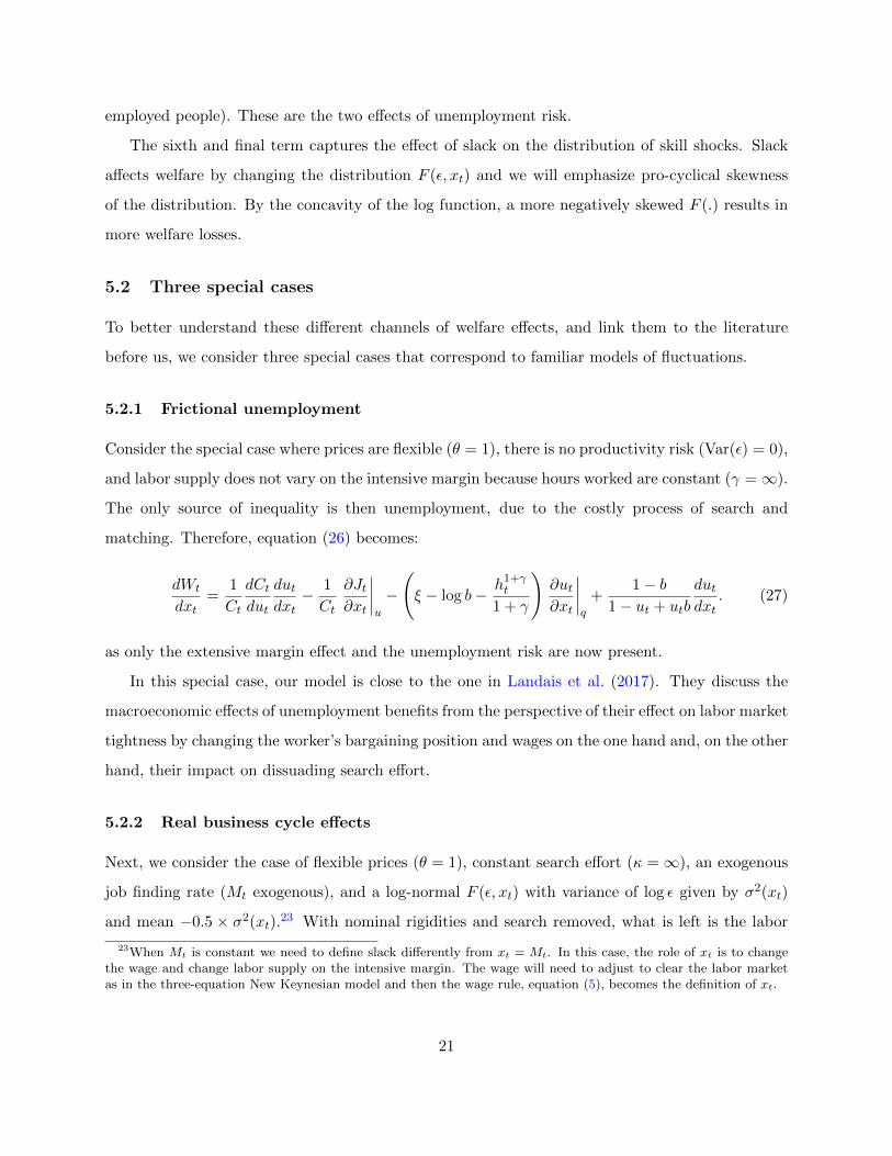
5.2 Three special cases

To better understand these different channels of welfare effects, and link them to the literature

before us, we consider three special cases that correspond to familiar models of fluctuations.

5.2.1 Frictional unemployment

Consider the special case where prices are flexible (θ = 1), there is no productivity risk (Var(ε) = 0),

and labor supply does not vary on the intensive margin because hours worked are constant (γ =∞).

The only source of inequality is then unemployment, due to the costly process of search and

matching. Therefore, equation (26) becomes:

dWt

dxt=

1

Ct

dCtdut

dutdxt− 1

Ct

∂Jt∂xt

∣∣∣∣u

−

(ξ − log b− h1+γ

t

1 + γ

)∂ut∂xt

∣∣∣∣q

+1− b

1− ut + utb

dutdxt

. (27)

as only the extensive margin effect and the unemployment risk are now present.

In this special case, our model is close to the one in Landais et al. (2017). They discuss the

macroeconomic effects of unemployment benefits from the perspective of their effect on labor market

tightness by changing the worker’s bargaining position and wages on the one hand and, on the other

hand, their impact on dissuading search effort.

5.2.2 Real business cycle effects

Next, we consider the case of flexible prices (θ = 1), constant search effort (κ =∞), an exogenous

job finding rate (Mt exogenous), and a log-normal F (ε, xt) with variance of log ε given by σ2(xt)

and mean −0.5 × σ2(xt).23 With nominal rigidities and search removed, what is left is the labor

23When Mt is constant we need to define slack differently from xt = Mt. In this case, the role of xt is to changethe wage and change labor supply on the intensive margin. The wage will need to adjust to clear the labor marketas in the three-equation New Keynesian model and then the wage rule, equation (5), becomes the definition of xt.

21

wedge and the effect of cyclical income risk on welfare, so equation (26) simplifies to

dWt

dxt= (1− ut)

[AtCt− hγt

]dhtdxt− β

1− β(1− τ)2 d

dxt

σ2(xt)

2. (28)

In this case, our paper fits into the standard analysis of business cycles in Chari et al. (2007)

through the first term, and into the study the costs of business cycles due to income inequality

emphasized by Krebs (2003) through the second term.

5.2.3 Aggregate demand effects

Traditionally, the literature on automatic stabilizers has focussed on aggregate demand effects

following a Keynesian tradition. When there is no productivity risk (Var(ε) = 0), job search effort

is constant (κ = ∞) and the labor market’s matching frictions are constant (Mt is constant),

equation (26) simplifies to:

dWt

dxt= (1− ut)

[AtCt− hγt

]dhtdxt− YtCtSt

dStdxt

,

so only the markup effects are present, both through the labor wedge and through price dispersion.

Appendix D.2 shows that a second-order approximation of Wt around the flexible-price, socially-

efficient level of aggregate output Y ∗t and consumption C∗t transforms this expression into

dWt

dxt=

(Y ∗tC∗t

)[(1

C∗t+

γ

Y ∗t

)(Y ∗t − YtY ∗t

)dYtdxt

+

(1− θθ

µ

µ− 1

)(Et−1pt − pt

Et−1pt

)dptdxt

],

In this case, our model fits into the new Keynesian framework with unemployment developed in

Blanchard and Galı (2010) or Gali (2011). Raising slack affects the output gap and the price

level, through the Phillips curve, and this affects welfare through the two conventional terms in the

expression. The first is the effect on the output gap, and the second the effect on surprise inflation.

These are the two sources of welfare costs in this economy.

5.3 Social programs and slack

We now turn attention to the second component of the macroeconomic stabilization term, either

dxt/db in the case of unemployment benefits, or dxt/dτ in the case of tax progressivity. Obtaining

22

analytical expressions for them is hard, unless extra assumptions are made. In Appendix E, we

characterize these terms by assuming that there is only aggregate uncertainty at date 0, that

household job search is exogenous, and that the income-risk distribution is log-normal. Here, we

discuss briefly the lessons from this very special case, which prove to be robust in our numerical

analysis.

Starting with dxt/db, there are two direct effects of raising unemployment benefits on economic

slack. The first is a classic redistribution effect: aggregate demand increases with an increase in

unemployment benefits because the unemployed have a high marginal propensity to consume. The

second is a precautionary effect: because unemployment benefits provide social insurance, they

lower uncertainty about the future, which reduces precautionary savings motive, and pushes up

aggregate demand today. Both of these effects become stronger in recessions, the first because

there are more unemployed receiving benefits, and the second because the risk of unemployment

and the corresponding precautionary savings motive rise during recessions. Unemployment benefits

therefore stimulate more during recessions, satisfying our criteria for an automatic stabilizer.

Turning to dxt/dτ , there is also a potentially important precautionary effect. When households

face uninsurable productivity risk, a progressive tax system will raise aggregate demand by reducing

the precautionary savings motive. This effect is counter-cyclical if risk increases in a recession, as

has been documented by Guvenen et al. (2014).

Like all fiscal policy, the effectiveness of the automatic stabilizers on economic activity further

depends on two other factors. The first one is the aggressiveness of monetary policy. A booming

economy leads to higher nominal interest rates, both directly via the Taylor rule and indirectly

via higher inflation. With nominal rigidities, this raises the real interest rate, which dampens the

effectiveness of any policy on equilibrium slack. An extreme example of this is when the economy

is at the zero lower bound, which magnifies the effectiveness of the automatic stabilizers.24 The

second factor is the extent of the counter-cyclicality of income risk. In response to a reduction in

aggregate demand, labor market tightness falls, leading to an increase in risk, and an increase in

the precautionary savings motive. This further reduces aggregate demand amplifying the business

cycle.25

24 McKay and Reis (2016) and Kekre (2017) show that automatic stabilizers and unemployment benefits, respec-tively, have stronger stimulating effects when the economy is at the zero lower bound.

25Similar reinforcing dynamics arise out of unemployment risk in Ravn and Sterk (2017), Den Haan et al. (2015),and Heathcote and Perri (2015).

23

5.4 Summary and likely sign

To summarize, there are two main channels through which unemployment benefits or income tax

progressivity raise aggregate demand and thereby eliminate slack. These channels are redistribution

and social insurance, and both are increasing in the unemployment rate. As unemployment and

income risks are counter-cyclical, these forces push for counter-cyclical elasticities of slack to the

social programs, since they dampen the counter-cyclical fluctuations in the precautionary savings

motive. If business cycles are inefficient in the sense that tightness is inefficiently low in a recession,

then we expect a positive covariance between dWt/dxt and the elasticities of tightness with respect

to policy. This positive covariance implies a positive aggregate stabilization term and more generous

unemployment benefits and a more progressive tax system even if the business cycle is efficient on

average.

6 Quantitative analysis

We have shown that the presence of business cycles leads to a macroeconomic stabilization term

in the determination of the optimal generosity of unemployment insurance and the progressivity

of income taxes, and that this term likely makes these programs more generous and progressive,

respectively. We now turn to numerical solutions in order to achieve three goals. First, we ask

whether the macroeconomic stabilization term is quantitatively significant. Second, we use the

analytical formulas presented above to understand the mechanisms driving the numerical results,

and to show that our three propositions can be applied to make sense of the results from more

complicated models.

The third goal is to evaluate the seven assumptions that we made in section 2 for analytical

tractability. Three of these cannot be kept while taking the model to fit the data. To generate

reasonable business cycles, we now allow for mortality, government spending shocks, and nominal

rigidity that lasts for more than one period through a Calvo pricing model. Therefore, we dispense

with Assumptions 1, 5, and 6. We also dispense with Assumption 3, and use the employment rate

as a measure of slack: xt = (1− ut)/(1− u). This maters little to the results because employment

and the job finding rate are highly correlated in the model, but this alternative assumption makes

the calibration more transparent because the unemployment rate is easily measured. The remaining

24

three assumptions—the wage rule, no public deficits, and no gross savings—are important also for

numerical tractability, so we maintain them for now, and then relax them one by one in section 6.5

to discuss their roles.

6.1 Calibration and solution of the general model

We solve the model using global methods, as described in Appendix F.2, so that we can accurately

compute social welfare, assuming that the economy starts at date 0 at the deterministic steady state.

We then numerically search for the values of b and τ that maximize the social welfare function, and

compare these with the maximal values in a counterfactual economy without aggregate shocks, but

otherwise identical.

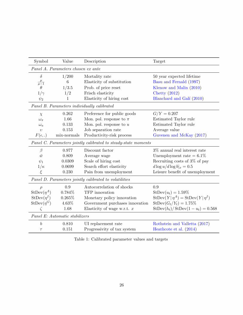
Table 1 shows the calibration of the model, dividing the parameters into different groups.

The first group has parameters set ex ante to standard choices in the literature. Only the last

one deserves some explanation. ψ2 is the elasticity of hiring costs with respect to labor market

tightness, and we set it at 1 as in Blanchard and Galı (2010), in order to be consistent with an

elasticity of the matching function with respect to unemployment of 0.5 as suggested by Petrongolo

and Pissarides (2001).

Panel B contains parameters individually calibrated to match time-series moments. For the

preference for public goods, we target the observed average ratio of government purchases to GDP

in the US in 1984-2007. For the monetary policy rule, we use OLS estimates of equation (6). The

parameter υ determines the probability of not having a job in our model, which we set equal to the

sum of quarterly job separation rate, which we construct following Shimer (2012), and the average

unemployment rate. Finally, we estimate a version of the income innovation process specified in

equation (2) using a mixture of normals as a flexible parameterization of the distribution F (ε′; ·).

Two of the mixture components shift with the unemployment rate to match the observed pro-

cyclical skewness of earnings growth rates documented by Guvenen et al. (2014). This parametric

income process is similar to the one in McKay (2017) and Guvenen and McKay (2017) and Appendix

F.1 provides additional details.26 As a check on our calibration, the model implies a cross-sectional

variance of log consumption of 0.40, while in 2005 CEX data the variance of log consumption of

non-durables was around 0.35 (Heathcote et al., 2010).

26We include unemployment fluctuations in the income process we simulate to match the empirical moments sothe contribution of unemployment to observed changes in income distributions is accounted for.

25

Symbol Value Description Target

Panel A. Parameters chosen ex ante

δ 1/200 Mortality rate 50 year expected lifetimeµµ−1 6 Elasticity of substitution Basu and Fernald (1997)

θ 1/3.5 Prob. of price reset Klenow and Malin (2010)1/γ 1/2 Frisch elasticity Chetty (2012)ψ2 1 Elasticity of hiring cost Blanchard and Galı (2010)

Panel B. Parameters individually calibrated

χ 0.262 Preference for public goods G/Y = 0.207ωπ 1.66 Mon. pol. response to π Estimated Taylor ruleωu 0.133 Mon. pol. response to u Estimated Taylor ruleυ 0.153 Job separation rate Average value

F (ε, .) mix-normals Productivity-risk process Guvenen and McKay (2017)

Panel C. Parameters jointly calibrated to steady-state moments

β 0.977 Discount factor 3% annual real interest ratew 0.809 Average wage Unemployment rate = 6.1%ψ1 0.0309 Scale of hiring cost Recruiting costs of 3% of pay1/κ 0.0699 Search effort elasticity d log u/d log b|x = 0.5ξ 0.230 Pain from unemployment Leisure benefit of unemployment

Panel D. Parameters jointly calibrated to volatilities

ρ 0.9 Autocorrelation of shocks 0.9StDev(ηA) 0.784% TFP innovation StDev(ut) = 1.59%StDev(ηI) 0.265% Monetary policy innovation StDev(Y | ηA) = StDev(Y | ηI)StDev(ηG) 4.63% Government purchases innovation StDev(Gt/Yt) = 1.75%

ζ 1.68 Elasticity of wage w.r.t. x StDev(ht)/ StDev(1− ut) = 0.568

Panel E: Automatic stabilizers

b 0.810 UI replacement rate Rothstein and Valletta (2017)τ 0.151 Progressivity of tax system Heathcote et al. (2014)

Table 1: Calibrated parameter values and targets

26

Panel C has parameters chosen jointly to target a set of moments. We target the average unem-

ployment rate between 1960 to 2014 and recruiting costs of 3 percent of quarterly pay, consistent

with Barron et al. (1997). The parameter κ controls the marginal disutility of effort searching for

a job, and we set it to target a micro-elasticity of unemployment with respect to benefits of 0.5 as

reported by Landais et al. (2017). Last in the panel is ξ, the non-pecuniary costs of unemployment.

In the model, the utility loss from unemployment is log(1/b) − h1+γ/(1 + γ) + ξ, reflecting the

loss in consumption, the gain in leisure, and other non-pecuniary costs of unemployment. We set

ξ = h1+γ/(1 + γ) in the steady state of our baseline calibration so that the benefit of increased

leisure in unemployment is dissipated by the non-pecuniary costs.

Panel D calibrates the three aggregate shocks in our model that perturb productivity, monetary

policy, and public expenditures. In each case, the exogenous process is an AR(1) in logs with

common autocorrelation. We set the variances to match three targets: (i) the standard deviation

of the unemployment rate, (ii) the standard deviation of Gt/Yt, and (iii) equal contributions of

productivity and monetary shocks to the variance of aggregate output. We set ζ = 1.68 to match

the standard deviation of hours per worker relative to the standard deviation of the employment-

population ratio.

Finally, panel E has the baseline values for the automatic stabilizers. For τ we adopt the

estimate of 0.151 from Heathcote et al. (2014). In calibrating b we target the observed degree

of insurance that households have against unemployment shocks, as measured by the change in

consumption upon unemployment. We set b = 0.81, consistent with a 19% decline in consumption

when unemployed since the literature has found consumption changes between 16% and 21%.27

These calibrated values for b and τ do not directly enter our analysis of optimal policy but are used

to jointly calibrate the other structural parameters of the model.

As a check on the model’s performance, the standard deviation of hours, output, and inflation

in the mode are 0.75%, 1.68%, and 0.65%. The equivalent moments in the US data 1960-2014 are

0.84%, 1.32%, and 0.55%.

27See Stephens Jr (2004), Aguiar and Hurst (2005), Saporta-Eksten (2014), and Chodorow-Reich and Karabarbou-nis (2016).

27

Steady state unemployment rate Standard deviation of log output

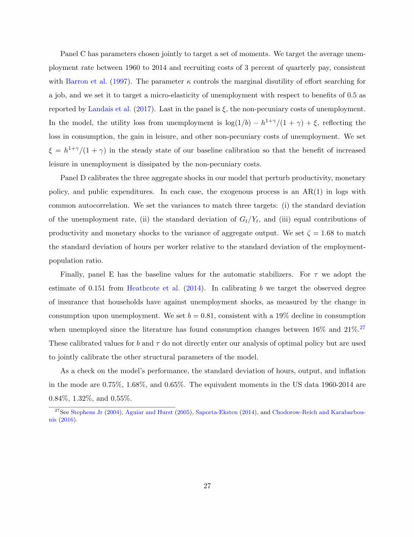
Figure 1: Effects of changing b for τ = 0.26

6.2 Optimal automatic stabilizers

Our first main quantitative result is that aggregate shocks increase the optimal b to 0.853 from

0.773 in the absence of aggregate shocks. Converting the values for b into pre-tax UI replacement

rates based on a two-earner household, then we have an optimal replacement rate of 61% with

aggregate shocks as compared to 41% percent without.28

Figure 1 provides a first hint for why this effect is so quantitatively large. It shows the effects

of raising b on the steady state unemployment rate and on the volatility of log output. Raising

the generosity of unemployment benefits hurts the incentives for working, so unemployment rises

somewhat. However, it has a strong macroeconomic stabilizing effect.

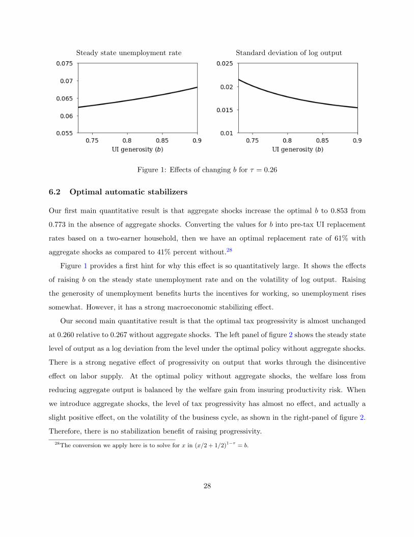
Our second main quantitative result is that the optimal tax progressivity is almost unchanged

at 0.260 relative to 0.267 without aggregate shocks. The left panel of figure 2 shows the steady state

level of output as a log deviation from the level under the optimal policy without aggregate shocks.

There is a strong negative effect of progressivity on output that works through the disincentive

effect on labor supply. At the optimal policy without aggregate shocks, the welfare loss from

reducing aggregate output is balanced by the welfare gain from insuring productivity risk. When

we introduce aggregate shocks, the level of tax progressivity has almost no effect, and actually a

slight positive effect, on the volatility of the business cycle, as shown in the right-panel of figure 2.

Therefore, there is no stabilization benefit of raising progressivity.

28The conversion we apply here is to solve for x in (x/2 + 1/2)1−τ = b.

28

Steady state output (log deviation) Standard deviation of log output

Figure 2: Effects of changing τ for b = 0.80. The left panel shows log output as a deviation fromthe value at τ = 0.267. The right panel uses the same vertical axis as figure 1 for comparison.

6.3 Using the analytical propositions to understand the numerical results

What drives the large automatic stabilization role for unemployment benefits, but not for income

tax progressivity? Our analytical results provide guidance on the key economic channels at play.

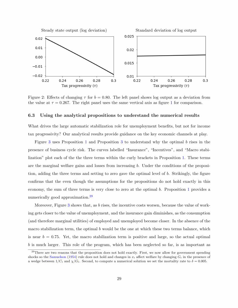
Figure 3 uses Proposition 1 and Proposition 3 to understand why the optimal b rises in the

presence of business cycle risk. The curves labelled “Insurance”, “Incentives”, and “Macro stabi-

lization” plot each of the the three terms within the curly brackets in Proposition 1. These terms

are the marginal welfare gains and losses from increasing b. Under the conditions of the proposi-

tion, adding the three terms and setting to zero gave the optimal level of b. Strikingly, the figure

confirms that the even though the assumptions for the propositions do not hold exactly in this

economy, the sum of three terms is very close to zero at the optimal b. Proposition 1 provides a

numerically good approximation.29

Moreover, Figure 3 shows that, as b rises, the incentive costs worsen, because the value of work-

ing gets closer to the value of unemployment, and the insurance gain diminishes, as the consumption

(and therefore marginal utilities) of employed and unemployed become closer. In the absence of the

macro stabilization term, the optimal b would be the one at which these two terms balance, which

is near b = 0.75. Yet, the macro stabilization term is positive and large, so the actual optimal

b is much larger. This role of the program, which has been neglected so far, is as important as

29There are two reasons that the proposition does not hold exactly. First, we now allow for government spendingshocks so the Samuelson (1954) rule does not hold and changes in xt affect welfare by changing Gt in the presence ofa wedge between 1/Ct and χ/Gt. Second, to compute a numerical solution we set the mortality rate to δ = 0.005.

29

Policy tradeoffs Components of macro stabilization term

Figure 3: Marginal welfare gain from changing b for τ = 0.26. The quantities in the left panelcorrespond to the terms in Proposition 1. The covariance term shows that the macroeconomicstabilization term is driven by the covariance term in equation (25). The terms in the right panelcorrespond to E0

∑∞t=0 β

t dWtdxt

dxtdb with dWt

dxtbroken into components as in Proposition 3. Both figures

are scaled to units of consumption equivalent welfare per unit change in b.

the incentives and redistribution roles that the literature has emphasized instead. A concern for

automatic stabilizers makes the unemployment insurance system significantly more generous.

The third and last striking result from Figure 3 is that the macroeconomic stabilization term is

driven by the covariance term in equation (25), not by the steady state inefficiency in the economy.

The benefits from stabilization do not come from closing the average gap between the level of

activity and its optimal level, but rather from attenuating the amplitude of the business cycle.

The right panel of Figure 3 unpacks the sources of the business-cycle stabilization benefits in

terms of the different sources of inefficient fluctuations that we characterized in Proposition 3. Each

curve in the figure corresponds to a component of the marginal welfare gain or loss from reducing

slack displayed in Proposition 3. The dominant component is clearly the reduction in idiosyncratic

risk that results from a higher b. By stabilizing the economy, more generous unemployment benefits

reduce the risk that households face in their pre-government incomes. This channel is distinct from

the insurance benefit, which is the smoothing of post-government income for a given risk to pre-

government income. The other components that are plotted in the figure, which reflect benefits

and losses in aggregate efficiency are all small in contrast. The inefficient utilization of labor on

the extensive margin is in fact negative, as raising b raises the unemployment rate on average.

Raising the progressivity of the income tax instead has a small macroeconomic stabilization

30

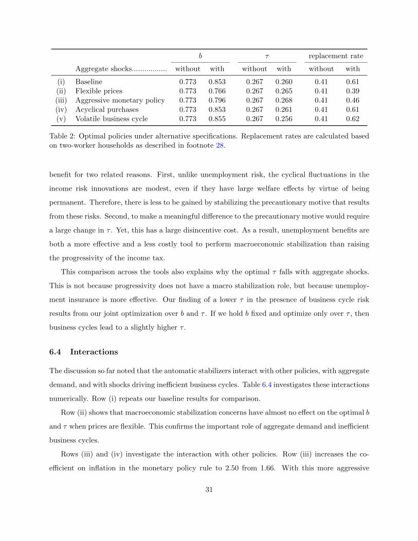
b τ replacement rate

Aggregate shocks................. without with without with without with

(i) Baseline 0.773 0.853 0.267 0.260 0.41 0.61(ii) Flexible prices 0.773 0.766 0.267 0.265 0.41 0.39(iii) Aggressive monetary policy 0.773 0.796 0.267 0.268 0.41 0.46(iv) Acyclical purchases 0.773 0.853 0.267 0.261 0.41 0.61(v) Volatile business cycle 0.773 0.855 0.267 0.256 0.41 0.62

Table 2: Optimal policies under alternative specifications. Replacement rates are calculated basedon two-worker households as described in footnote 28.

benefit for two related reasons. First, unlike unemployment risk, the cyclical fluctuations in the

income risk innovations are modest, even if they have large welfare effects by virtue of being

permanent. Therefore, there is less to be gained by stabilizing the precautionary motive that results

from these risks. Second, to make a meaningful difference to the precautionary motive would require

a large change in τ . Yet, this has a large disincentive cost. As a result, unemployment benefits are

both a more effective and a less costly tool to perform macroeconomic stabilization than raising

the progressivity of the income tax.

This comparison across the tools also explains why the optimal τ falls with aggregate shocks.

This is not because progressivity does not have a macro stabilization role, but because unemploy-

ment insurance is more effective. Our finding of a lower τ in the presence of business cycle risk

results from our joint optimization over b and τ . If we hold b fixed and optimize only over τ , then

business cycles lead to a slightly higher τ .

6.4 Interactions

The discussion so far noted that the automatic stabilizers interact with other policies, with aggregate

demand, and with shocks driving inefficient business cycles. Table 6.4 investigates these interactions

numerically. Row (i) repeats our baseline results for comparison.

Row (ii) shows that macroeconomic stabilization concerns have almost no effect on the optimal b

and τ when prices are flexible. This confirms the important role of aggregate demand and inefficient

business cycles.

Rows (iii) and (iv) investigate the interaction with other policies. Row (iii) increases the co-

efficient on inflation in the monetary policy rule to 2.50 from 1.66. With this more aggressive

31

monetary policy rule there is less of a need for fiscal policy to manage aggregate demand. There-

fore, stabilization plays a smaller role in the design of the optimal social insurance system than

in the baseline calibration. Moreover, flexible prices or aggressive monetary policy make the real

interest rate responds strongly to changes in slack. The elasticities of slack with respect to the

social programs is small leading to a small automatic-stabilizer role.

Row (iv) changes instead the policy rule for government purchases. Our baseline specification,

following the Samuelson rule, makes government purchases pro-cyclical. Row (iv) considers instead

acyclical government purchases, as we observe in the data, by using instead the rule: Gt = GηGt .

While the pro-cyclical rule amplifies the business cycle and leaves a larger role for the automatic

stabilizers, the effect is quantitatively minor.

Rows (v) shows that the calibration of the aggregate shocks is not crucial to our results. Row

(v) raises the standard deviations of the productivity and monetary policy shocks by 25%. As one

might expect, when the aggregate shocks are more volatile, stabilization plays a larger role in the

choice of b and τ , but the difference is minor. What is important for our results is the degree of

internal amplification of shocks through precautionary savings effects on aggregate demand. While

the results are sensitive to the degree of price flexibility and the monetary policy rule, they are not

so sensitive to the exact nature of the shocks hitting the economy.

6.5 Evaluating our simplifying assumptions

We have maintained three simplifying assumptions for tractability: a particular wage rule, a bal-

anced government budget, and assets in zero gross supply leading to no private savings in equilib-

rium. We now relax each of these in turn.

6.5.1 The wage rule

There are two features of wages that are especially important for the effectiveness of the stabilizers.

The first is the cyclicality of wages, since this affects the amplitude of the business cycle. The

second is whether there is a direct response of wages to changes in policy, as changes in benefits or

take-home pay affect that bargaining power of workers.

In our wage rule, the parameter ζ captures the elasticity of wages with respect to slack. Making

the wage more cyclical makes the intensive margin of labor supply more volatile while the unemploy-

32

ment rate (the extensive margin) becomes less volatile. With less variability in the unemployment

rate there is less amplification through the precautionary savings motive, and so less value in using

the automatic stabilizers to stabilize the business cycle. When we double ζ, the optimal b is now

only 0.804, and increases with business cycles only by 0.031. While this change reduces the role of

the automatic stabilizers, it implies a counterfactually low level of unemployment volatility.

In the baseline specification, the steady state wage barely changes across policy regimes, since

policy only affects the costs of hiring in the term 1− Jt/Yt, which is quite small in practice. This

specification is consistent with empirical work that fails to find an effect of unemployment benefits

on wages.30 However, some studies have found large effects of unemployment benefits on the

equilibrium unemployment rate possibly reflecting general equilibrium effects operating through

wages (Hagedorn et al., 2013). We explore how our analysis is affected when the steady state wage

is increasing in the unemployment benefit, by assuming that w has an elasticity of 0.1 with respect

to b.

With a positive wage elasticity, the steady state unemployment rate increases with the benefits

more strongly than before. Higher benefits raise wages, which lowers the incentives for firms to

hire workers, leading to a lower job-finding rate. Moreover, the incentives for searching for a job

fall both because of the usual moral hazard effect and due to the decline in the job-finding rate.

With a positive wage elasticity, the greater sensitivity of the steady state unemployment rate to

the unemployment benefit leads to much lower optimal benefits in the absence of aggregate shocks:

0.53 as opposed to 0.77 in our baseline.

However, when there are aggregate shocks, low benefits lead to strong de-stabilizing dynamics

because of the precautionary savings motive. Because there is little social insurance, the precau-

tionary savings motive is stronger and more cyclical, which leads to stronger internal amplification

of shocks so fluctuations become costlier. The automatic-stabilizer nature of unemployment bene-

fits is therefore substantially stronger. As a result, in this case we find that aggregate shocks lead

to a large change in the optimal benefit relative to what is optimal in steady state: the optimal

b rises from 0.53 to 0.73 with aggregate shocks. Therefore, a positive wage elasticity with respect

to benefits leads to lower replacement rates overall, but a larger effect of the business cycle on the

optimal policy.

30Card et al. (2007), Van Ours and Vodopivec (2008), Lalive (2007), and Johnston and Mas (2015) find no evidencethat UI generosity affects earnings upon re-employment.

33

6.5.2 Budget deficits

The baseline analysis assumed a balanced budget, which was achieved by having the average tax

rate respond to any shocks to fiscal revenues or expenditures. Because of the way in which we

specified the tax function, it is the progressivity (τ) rather than the level (λt) that drives the

willingness to work or consume, as shown in section 3. Still, one may worry that public deficits

during recessions may, through an effect on aggregate demand, further enhance the effectiveness of

the stabilizers. To allow for this possibility, while still maintaining the aggregation result that there

is a zero gross supply of domestic assets, we now allow for the government to borrow from foreigners.

In particular, we assume the government can borrow at a world interest rate R∗ = 1.031/4, so the

government budget constraint now is:

Gt +R∗Bt =

∫ni,t

(zi,t − λtz1−τ

i,t

)− (1− ni,t) bλtz1−τ

i,t di+Bt+1

The fiscal policy rule for taxes is now not to balance the budget at every date, but rather to

gradually pay for the public debt:31

λt = λ

(λ∗tλ

)−`λ− `B

BtY,

where λ∗t is the level of λt that results in a balanced budget in period t and 1− λ is the steady state

level of taxes. We set the parameter `λ = 0.5 to match the standard deviation of public deficits to

GDP, which is 0.9%. The parameter `B = 0.1 makes the public debt stationary, and its value is set

to match the high persistence of the observed debt-to-GDP ratio.

Allowing for foreign borrowing has only a minor impact on the results. The optimal b without

business cycles now is 0.773 and the optimal b with business cycles is 0.852, while the respective

numbers for τ are 0.267 and 0.263. While a public deficit results in a current account deficit

that is capable of stabilizing aggregate consumption, it does not necessarily stabilize production or

employment. Because idiosyncratic risk, which is crucial for our welfare considerations, is driven by

labor demand, the deficits do not reduce the need to stabilize production. While deficits are helpful

in stabilizing aggregate consumption, that is not the main rationale for stabilizing the economy.

31Recall that after tax income is λtz1−τi,t where zi,t is pre-tax income so the average tax rate is decreasing in λ.

34

Standard deviation log Yt Steady state unemployment

Figure 4: Standard deviation of log output and steady state unemployment rate as functions ofinsurance against unemployment shocks for different levels of savings. Insurance is defined asthe percentage difference between E[u′(c)|unemployed] and E[u′(c)|employed] in steady state. Thenumbers labeling the lines give the value of b that corresponds to that level of insurance.

6.5.3 Aggregate borrowing and saving

Finally, we drop the last assumption that there are no assets in gross supply. This was important

so far to keep both the analytical and the numerical models tractable, since we did not have to keep

track of a changing wealth distribution. The key new assumption is that now there is a constant

and policy-invariant positive stock of government debt that private households can hold to self

insure against unemployment shocks, so now there is a distribution of wealth that changes over

time and responds to policy. The level of taxes adjusts to keep this stock of debt constant, so there

are no deficits, which were studied in the previous sub-section. Appendix G provides a detailed

description of the equilibrium conditions of the extended model, which we solve using the Reiter

(2009) method, which gives a non-linear solution with respect to idiosyncratic state variables, but a

linearized solution with respect to aggregate states. To keep the computational burden manageable,

we focus on unemployment benefits and unemployment risk by shutting off the productivity risk.

The left panel of Figure 4 shows how the volatility of the economy in terms of the standard

deviation of log output is related to the steady state level of the insurance against unemployment

that households have. This is measured in the horizontal axis in terms of the average difference

in marginal utilities between the employed and the unemployed, so a larger difference in marginal

utilities corresponds to less insurance. Moving along a curve in the figure varies the generosity of

unemployment benefits, indicated by the labels, and so the insurance that households have against

unemployment, while holding the aggregate level of savings constant. Each curve corresponds to

35

a different level of total savings in the economy, obtained by varying the discount factor β, while

keeping fixed the annual interest rate at 2%. The right panel of Figure 4 shows a similar plot but

with the steady state unemployment rate on the vertical axis.

The left panel of Figure 4 shows that, for a given level of insurance (a point on the x-axis)

the slopes of the volatility lines are quite similar across levels of savings. Therefore, the marginal

benefit in terms of stabilizing the economy from providing more insurance through the UI system

changes little across levels of savings. In turn, the right panel shows that the same applies with

respect to the marginal incentive cost, since the increase in the unemployment rate reflected in the

slopes of the curves again barely changes with the level of savings. Therefore, the macroeconomic

stabilization term will be similar to our baseline, and so will be the effect of business cycles on

optimal unemployment insurance.

Calculating the optimal b in the model with savings turns out to not be too informative because,

since we now omit the time-varying productivity risk, we are leaving out a key determinant of

welfare. Instead, we pick b to maximize an ad hoc objective function: V (b) + Vσσ(b), where V (b)

is steady state welfare, σ(b) is the standard deviation of log output and Vσ is a parameter that

stands in for the value of output stabilization that comes from time-varying productivity risk in

the baseline model. We set Vσ so that if there is no savings (and no productivity risk), then the

optimal b and insurance level match the optimum in our baseline model.

Table 3 shows the results from maximizing this objective function. The first interesting lesson

is that, with savings but no business cycles, the optimal unemployment benefit is less generous.

Agents partly self-insure now, so they do need as much social insurance. Second, introducing

business cycles makes a larger difference to the optimal b and the extent of under-insurance with

savings than without them. While savings reduce the marginal benefit of social insurance, they

also reduce the disincentive effect of benefits on working. As Figure 4 highlighted, the end effect is

that the trade-off between insurance and incentives ends up being quite stable in spite of savings.

7 Conclusion

Policy debates take as given that there are stabilizing benefits of unemployment insurance and

income tax progressivity, but there are few systematic studies of what factors drive these benefits

and how large they are. In contrast, the study of these social programs in the academic literature

36

Without aggregate shocks With aggregate shocks

b Under-insurance b Under-insurance

Baseline 0.773 0.294 0.853 0.172No savings, ad hoc objective 0.780 0.283 0.853∗ 0.172∗

Savings, ad hoc objective 0.600 0.406 0.741 0.168

Table 3: Optimal policies with and without savings. Under-insurance is defined as the percentagedifference between E[u′(c)|unemployed] and E[u′(c)|employed] in steady state. ∗ indicates that thead hoc objective function is designed to match the optimal policy in the baseline model.

rarely takes into account this macroeconomic stabilization role, instead treating it as a fortuitous

side benefit.

This paper tries to remedy this situation. Our theoretical study provides a theoretical charac-

terization of what is an automatic stabilizer. In general terms, an automatic stabilizer is a fixed

policy for which there is a positive covariance between the effect of slack on welfare, and the effect of

the policy on slack. If a policy tool has this property of stimulating the economy more in recessions

when slack is inefficiently high, then its role in stabilizing the economy calls for expanding the use

of the policy beyond what would be appropriate in a stationary environment. Overall, we found

that the role of social insurance programs as automatic stabilizers affects their optimal design and,

in the case of unemployment insurance, it can lead to substantial differences in the generosity of

the system.

Our focus on the automatic stabilizing nature of existing social programs led us to take a

Ramsey approach to the ex ante design of fiscal policy. Future work might explore how these

forces affect the design of the social insurance system from a Mirrleesian perspective. Another

question is how these fiscal policy programs can adjust to the state of the business cycle, taking

into account measurement difficulties, time inconsistency, political economy, and other challenges

of implementing state-dependent stabilization policy. There is already some progress on these two

topics, and hopefully our analysis will provide some insights to guide their further development.

37

References

Aguiar, M. and Hurst, E. (2005). Consumption versus expenditure. Journal of Political Economy, 113(5):919–948.

Aiyagari, S. R. and McGrattan, E. R. (1998). The optimum quantity of debt. Journal of Monetary Eco-nomics, 42(3):447–469.

Auclert, A. (2016). Monetary policy and the redistribution channel. Princeton University manuscript.

Auerbach, A. J. and Feenberg, D. (2000). The significance of federal taxes as automatic stabilizers. Journalof Economic Perspectives, 14(3):37–56.

Baily, M. N. (1978). Some aspects of optimal unemployment insurance. Journal of Public Economics,10(3):379–402.

Barron, J. M., Berger, M. C., and Black, D. A. (1997). On-the-job training. W.E. Upjohn Institute forEmployment Research, Kalamazoo, MI.

Basu, S. and Fernald, J. G. (1997). Returns to scale in US production: Estimates and implications. Journalof Political Economy, 105(2):249–283.

Benabou, R. (2002). Tax and education policy in a heterogeneous agent economy: What levels of redistri-bution maximize growth and efficiency? Econometrica, 70(2):481–517.

Bhandari, A., Evans, D., Golosov, M., and Sargent, T. J. (2017). Inequality, business cycles and fiscal-monetary policy. University of Minnesota working paper.

Blanchard, O., Dell’Ariccia, G., and Mauro, P. (2010). Rethinking macroeconomic policy. Journal of Money,Credit and Banking, 42(s1):199–215.

Blanchard, O. and Galı, J. (2010). Labor markets and monetary policy: A New Keynesian model withunemployment. American Economic Journal: Macroeconomics, 2(2):1–30.

Card, D., Chetty, R., and Weber, A. (2007). Cash-on-hand and competing models of intertemporal behavior:New evidence from the labor market. Quarterly Journal of Economics, 122(4):1511–1560.

Chari, V. V., Kehoe, P. J., and McGrattan, E. R. (2007). Business cycle accounting. Econometrica, 75(3):781–836.

Chetty, R. (2006). A general formula for the optimal level of social insurance. Journal of Public Economics,90(10):1879–1901.

Chetty, R. (2012). Bounds on elasticities with optimization frictions: A synthesis of micro and macroevidence on labor supply. Econometrica, 80(3):969–1018.

Chodorow-Reich, G. and Karabarbounis, L. (2016). The cyclicality of the opportunity cost of employment.Journal of Political Economy, 124(6):1563–1618.

Conesa, J. C. and Krueger, D. (2006). On the optimal progressivity of the income tax code. Journal ofMonetary Economics, 53(7):1425–1450.

De Santis, M. (2007). Individual consumption risk and the welfare cost of business cycles. American EconomicReview, 97(4):1488 – 1506.

Den Haan, W. J., Rendahl, P., and Riegler, M. (2015). Unemployment (fears) and deflationary spirals.CEPR Discussion Paper 10814.

38

DiMaggio, M. and Kermani, A. (2016). The importance of unemployment insurance as an automatic stabi-lizer. Columbia Business School Research Paper 15-31.

Gali, J. (2011). Unemployment Fluctuations and Stabilization Policies: A New Keynesian Perspective. MITPress, Cambridge, USA.

Galı, J., Gertler, M., and Lopez-Salido, J. D. (2007). Markups, gaps, and the welfare costs of businessfluctuations. The Review of Economics and Statistics, 89(1):44–59.

Golosov, M., Troshkin, M., and Tsyvinski, A. (2016). Redistribution and social insurance. AmericanEconomic Review, 106(2):359–386.

Guerrieri, V. and Lorenzoni, G. (2011). Credit crises, precautionary savings, and the liquidity trap. NBERWorking Paper 17583.

Guvenen, F., Karahan, F., Ozkan, S., and Song, J. (2015). What do data on millions of U.S. workers revealabout life-cycle earnings risk? University of Minnesota working paper.

Guvenen, F. and McKay, A. (2017). A parsimonious income process for business cycle analysis. BostonUniversity Working Paper.

Guvenen, F., Ozkan, S., and Song, J. (2014). The nature of countercyclical income risk. Journal of PoliticalEconomy, 122(3):pp. 621–660.

Hagedorn, M., Karahan, F., Manovskii, I., and Mitman, K. (2013). Unemployment benefits and unemploy-ment in the great recession: The role of macro effects. NBER Working Paper 19499.

Hall, R. E. (2005). Employment fluctuations with equilibrium wage stickiness. American Economic Review,95(1):50–65.

Heathcote, J. and Perri, F. (2015). Wealth and volatility. NBER Working Paper 20944.

Heathcote, J., Perri, F., and Violante, G. L. (2010). Unequal we stand: An empirical analysis of economicinequality in the united states, 1967–2006. Review of Economic dynamics, 13(1):15–51.

Heathcote, J., Storesletten, K., and Violante, G. L. (2014). Optimal Tax Progressivity: An AnalyticalFramework. NBER working paper 19899.

Hosios, A. J. (1990). On the efficiency of matching and related models of search and unemployment. Reviewof Economic Studies, 57(2):279–298.

IMF (2015). Can fiscal policy stabilize output? In Fiscal Monitor, chapter 2, pages 21–49. InternationalMonetary Fund.

Johnston, A. C. and Mas, A. (2015). Potential unemployment insurance duration and labor supply: theindividual and market-level response to a benefit cut. Princeton University working paper.

Jung, P. and Kuester, K. (2015). Optimal labor-market policy in recessions. American Economic Journal:Macroeconomics, 7(2):124–156.

Kaplan, G. W., Moll, B., and Violante, G. (2016). Monetary policy according to HANK. Princeton Universitymanuscript.

Kekre, R. (2017). Unemployment insurance in macroeconomic stabilization. University of Chicagomanuscript.

39

Klenow, P. J. and Malin, B. A. (2010). Microeconomic evidence on price-setting. In Friedman, B. andWoodford, M., editors, Handbook of Monetary Economics, volume 3A, pages 231–284. Elsevier: NorthHolland.

Krebs, T. (2003). Growth and welfare effects of business cycles in economies with idiosyncratic human capitalrisk. Review of Economic Dynamics, 6(4):846–868.

Krebs, T. (2007). Job displacement risk and the cost of business cycles. American Economic Review,97(3):664–686.

Krueger, D. and Ludwig, A. (2013). Optimal progressive labor income taxation and education subsidieswhen education decisions and intergenerational transfers are endogenous. American Economic Review,103(3):496–501.

Krusell, P., Mukoyama, T., and Smith, Jr., A. A. (2011). Asset prices in a Huggett economy. Journal ofEconomic Theory, 146(3):812–844.

Lalive, R. (2007). Unemployment benefits, unemployment duration, and post-unemployment jobs: A regres-sion discontinuity approach. American Economic Review, 97(2):108–112.

Landais, C., Michaillat, P., and Saez, E. (2017). A macroeconomic approach to optimal unemploymentinsurance i: Theory. American Economic Journal: Economic Policy.

Maliar, L. and Maliar, S. (2015). Merging simulation and projection approaches to solve high-dimensionalproblems with an application to a new Keynesian model. Quantitative Economics, 6(1):1–47.

Mankiw, N. G. and Reis, R. (2010). Imperfect information and aggregate supply. In Friedman, B. andWoodford, M., editors, Handbook of Monetary Economics, volume 3A, chapter 5, pages 183–230. Elsevier:North Holland.

McKay, A. (2017). Time-varying idiosyncratic risk and aggregate consumption dynamics. Journal of Mon-etary Economics, 88:1–14.

McKay, A., Nakamura, E., and Steinsson, J. (2016). The power of forward guidance revisited. AmericanEconomic Review, 106(10):3133–3158.

McKay, A. and Reis, R. (2016). The role of automatic stabilizers in the U.S. business cycle. Econometrica,84(1):141–194.

Mirrlees, J. A. (1971). An exploration in the theory of optimum income taxation. Review of EconomicsStudies, 38(2):175–208.

Mitman, K. and Rabinovich, S. (2011). Pro-cyclical unemployment benefits? optimal policy in an equilibriumbusiness cycle model. PIER working paper 11-010.

Musgrave, R. A. and Miller, M. H. (1948). Built-in flexibility. American Economic Review, 38(1):122–128.

Oh, H. and Reis, R. (2012). Targeted transfers and the fiscal response to the great recession. Journal ofMonetary Economics, 59(Supplement):S50–S64.

Perotti, R. (2005). Estimating the effects of fiscal policy in OECD countries. Federal Reserve Bank of SanFrancisco, Conference Proceedings.

Petrongolo, B. and Pissarides, C. A. (2001). Looking into the black box: A survey of the matching function.Journal of Economic Literature, 39:390–431.

40

Ravn, M. and Sterk, V. (2017). Job uncertainty and deep recessions. Journal of Monetary Economics,90:125–141.

Reiter, M. (2009). Solving heterogeneous-agent models by projection and perturbation. Journal of EconomicDynamics and Control, 33(3):649–665.

Rothstein, J. and Valletta, R. G. (2017). Scraping by: Income and program participation after the loss ofextended unemployment benefits. Journal of Policy Analysis and Management., forthcoming.

Samuelson, P. A. (1954). The pure theory of public expenditure. The Review of Economics and Statistics,36(4):387–389.

Saporta-Eksten, I. (2014). Job loss, consumption and unemployment insurance. Tel-Aviv University WorkingPaper.

Shimer, R. (2012). Reassessing the ins and outs of unemployment. Review of Economic Dynamics, 15(2):127– 148.

Stephens Jr, M. (2004). Job loss expectations, realizations, and household consumption behavior. TheReview of Economics and Statistics, 86(1):253–269.

Storesletten, K., Telmer, C. I., and Yaron, A. (2001). The welfare cost of business cycles revisited: Finitelives and cyclical variation in idiosyncratic risk. European Economic Review, 45(7):1311–1339.

Storesletten, K., Telmer, C. I., and Yaron, A. (2004). Cyclical dynamics in idiosyncratic labor market risk.Journal of Political Economy, 112(3):695–717.

Van Ours, J. C. and Vodopivec, M. (2008). Does reducing unemployment insurance generosity reduce jobmatch quality? Journal of Public Economics, 92(3):684–695.

Varian, H. R. (1980). Redistributive taxation as social insurance. Journal of Public Economics, 14(1):49–68.

Werning, I. (2007). Optimal fiscal policy with redistribution. Quarterly Journal of Economics, 122(3):925–967.

Werning, I. (2015). Incomplete markets and aggregate demand. NBER Working Paper 21448.

Woodford, M. (2010). Optimal monetary stabilization policy. In Friedman, B. M. and Woodford, M., editors,Handbook of Monetary Economics, volume 3, chapter 14, pages 723 – 828. Elsevier: North Holland.

41

Appendix

This appendix contains five sections, which: describe the role of the wage rule introduced in

section 2; provide auxiliary steps to some results stated in section 3; prove the propositions in

sections 4; derive the AD-AS apparatus and prove the propositions in section 5; and describe the

methods used to solve the model in section 6.

A The wage rule

This section first describes a bargaining protocol that gives rise to the wage rule we assumed, and

next modifies our analytical results to allow for a non-isoelastic wage rule.

A.1 Nash bargaining protocol and our wage rule

This appendix presents a Nash bargaining protocol that gives rise to our wage rule. To define

a Nash bargaining solution we have to define the outside options of the firm and the worker. If

bargaining breaks down, we assume that the firm can obtain a different worker by paying the hiring

cost again and the worker can meet another firm but loses some of the period’s time endowment.

Let zt be the amount of time lost if bargaining breaks down. One could assume that zt is a constant

parameter (e.g. it takes a given amount of time to meet a new firm once bargaining breaks down)

or one could assume that it is easier to find a new firm when the labor market is tight or more

productive zt = zA−1M−ιt . The worker chooses total market time, h, before bargaining begins. If

bargaining breaks down, we assume the next employer pays the equilibrium wage (i.e. we do not

consider bargaining in that relationship). We assume that employed workers of a given skill are

able to pool the gains from bargaining between themselves (in equilibrium they all negotiate the

same wage so there are no transfers, but this means that bargaining does not take into account the

curvature of the individual utility function or the non-linearity of the tax system).

The surplus to a worker of an offer that pays w when the market wage is w is

V (w, w, α) = µV (α)α [wh− w(h− z)] ,

where µV (α) is the marginal valuation of resources by the employed workers of skill α. The surplus

42

to the firm is

J(w, w, α) = µJα[ψ1M

ψ2 + wh− wh],

where µJ is the marginal valuation of resources by the firm. In the firm’s surplus we assume hiring

costs are proportional to α, which is consistent with our assumption that hiring an effective unit of

labor costs ψ1Mψ2 because the average α in the employed and unemployed populations is always

constant at one.

The generalized Nash bargaining solution satisfies

maxw

V (w, w, α)ℵJ(w, w, α)1−ℵ

where ℵ is the worker’s bargaining power. The first order condition at w = w is

ℵ1− ℵ

µJψ1Mψ2hµV (α)α2 = µJhµV (α)wzα2

ℵ1− ℵ

ψ1Mψ2 = wz

Substituting z = A−1M−ι

w =1

z

ℵ1− ℵ

ψ1AMψ2+ι (29)

Now set z and ℵ such that 1zℵ

1−ℵψ1 = wM−ζ and set ι such that ψ2 + ι = ζ. The result is that this

bargaining protocol gives rise to our wage rule except for the (1−J/Y ) term, which is quantitatively

innocuous. If zt fluctuates in a more complicated manner, we can derive a wage rule that includes

the (1− J/Y ) term.

A.2 The role of the wage rule in our analysis

We assumed that the wage was determined by equation (5). A more general specification uses a

generic wage function:

wt = w(ηt, xt, b, τ),

43

that maps the aggregate shocks, slack (or labor market tightness), and policy parameters into a

wage.

In this more general case, we can write ht as:

ht =

(1− τ)

[ηAtS(xt)

(1− Jt

Yt

)]−1

w(ηAt , xt, b, τ)

1/(1+γ)

where S(xt) is the level of price dispersion associated with that level of slack. Using the generic

wage rule and equations (3), (4), (19), (21), (36), and (38), we can write Jt/Yt as a function of

(ηt, xt, b, τ) to yield:

ht = (1− τ)H(ηt, xt, b, τ)1/(1+γ) ,

where Ht ≡[

ηtS(xt)

(1− Jt

Yt

)]−1w(ηt, xt, b, τ). The purpose of assuming the wage rule in equation

(5) in the paper is that Ht simplifies to xζt .

However, not making this simplification, and so carrying the new H(.) term along only adds

to our results a few additional terms. To start, in addition to those terms that appear in equation

(23) (Proposition 1), we would now need to add:

E0

∞∑t=0

βt(1− ut)[AtCt− hγt

]dhtdHt

∂Ht

∂b

∣∣∣∣x

.

Similarly, we would need to modify equation (24) (Proposition 2) to include a term:

E0

∞∑t=0

βt(1− ut)[AtCt− hγt

]dhtdHt

∂Ht

∂τ

∣∣∣∣x

.

Both of these terms relate to the adjustment of hours on the intensive margin. Intuitively, the

wage plays two roles in the economy: it determines the marginal cost of the firms and therefore

the incentives for hiring and it determines the incentives for labor supply on the intensive margin.

The first effect is captured in our analysis through dxt/db. Using our wage rule, the second effect

is captured through dhtdxt

dxtdb . A more general wage rule brings in these new effects of policy on

intensive margin labor supply. A different wage rule would also result in different values for dxt/db

and dxt/dτ , but these are not qualitatively different considerations than the ones we focus on

44

already.

B Additional steps for deriving the results in section 3

B.1 The value of employment

In equilibrium, ai,t = 0, and search effort is determined by comparing the value of working and not

working according to equation (14). This section of the appendix derives the two key steps that

make this difference independent of the household’s type, so that all households choose the same

search effort.

Lemma 3. Suppose the household’s value function has the form

V (α, n,S) = V α(α,S) + V n(a, n,S)

for some functions V α and V n where S is the aggregate state. The choice of search effort is then

the same for all searching households regardless of α.

Proof: The household’s search problem is

V s(α,S) = maxq

MqV (α, 1,S) + (1−Mq)V (α, 0,S)− q1+κ

1 + κ

.

Substitute for the value functions to arrive at

V s(α,S) = maxq

Mq [V α(α,S) + V n(a, 1,S)] + (1−Mq) [V α(α,S) + V n(a, 0,S)]− q1+κ

1 + κ

V s(α,S) = V α(α,S) + max

q

MqV n(1,S) + (1−Mq)V n(0,S)− q1+κ

1 + κ

, (30)

where we have brought V α(α,S) outside the max operator as it appears in an additively separable

manner. As there is no α inside the max operator, the optimal q is independent of α.

Lemma 4. The household’s value function can be written as

V (α, n,S) =1− τ1− β

log(α) + n

[log

1

b− h1+γ

1 + γ+ ξ

]+ V (S) (31)

for some function V .

45

Proof. Suppose that the value function is of the form given in (31). We will establish that the

Bellman equation maps functions in this class into itself, which implies that the fixed point of the

Bellman equation is in this class by the contraction mapping theorem. V s will then be

V s(α,S) =1− τ1− β

log(α) +Mq∗[log

1

b− h1+γ

1 + γ+ ξ

]− q∗1+κ

1 + κ+ V (S)

and the choice of q∗ is independent of α by Lemma 3. Regardless of employment status, the

continuation value is

(1− υ)V (α′, 1,S ′) + υV s(α′,S ′)

= (1− υ)

[1− τ1− β

log(α′) +

[log

1

b− h′1+γ

1 + γ+ ξ

]+ V (S ′)

]

+ υ

[1− τ1− β

log(α′) +M ′q∗′[

log1

b− h′1+γ

1 + γ+ ξ

]− q∗′

1+κ

1 + κ+ V (S ′)

]=

1− τ1− β

log(α′) + g(S ′),

where

g(S) ≡ (1− υ + υM ′q∗′)

[log

1

b− h′1+γ

1 + γ

]− (1− υ)

q∗′1+κ

1 + κ+ V (S ′).

Turning to the Bellman equation, we have

V (α, n,S) = log[λ(n+ (1− n)b) (α(wh+ d))1−τ

]− n h

1+γ

1 + γ− (1− n)ξ + βE

[1− τ1− β

log(α′) + g(S ′)]

=1− τ1− β

log(α) + n

[log

1

b− h1+γ

1 + γ+ ξ

]+ log

[λ (wh+ d)1−τ

]+ log b− ξ + β

1− τ1− β

E[log(ε′)

]+ βE

[g(S ′)

].

Finally, V (S) is given by the second row of the expression above.

B.2 Proof of lemma 2

First, the Euler equation for a household is

1

ci,t≥ βRtE

[1

ci,t+1

].

46

as usual. At the same time, as we showed in the text, the consumption of an individual is

ci,t = λtα1−τi,t (wtht + dt)

1−τ (ni,t + (1− ni,t)b). (32)

Replacing individual consumption into the Euler equation, and rewriting gives:

1

λt (wtht + dt)1−τ ≥ βRtEt

(1− ut+1) + ut+1b

−1

λt+1 (wt+1ht+1 + dt+1)1−τ

Et

[α1−τi,t

α1−τi,t+1

][ni,t + (1− ni,t)b] . (33)

Notice that E[α1−τi,t

α1−τi,t+1

]= E

[ετ−1i,t+1

]is common across households. This Euler equation only dif-

fers across households due to the final term involving ni,t. Assuming the unemployment benefit

replacement rate is less than one, this term will be larger for employed than unemployed so in

equilibrium all unemployed will be constrained and the Euler equation will hold with equality for

all employed.32

Summing equation (32) across households gives:

Ct = λt (wtht + dt)1−τ (1− ut + utb)Ei

[α1−τi,t

]. (34)

Solve (34) for λt (wtht + dt)1−τ and substitute it into (32) to arrive at:

ci,t = α1−τi,t (ni,t + (1− ni,t)b)

Ct

(1− ut + utb)Ei[α1−τi,t

] . (35)

Equations (15) and (20) follow from (35) and the definition of ct.

To derive equations (16) and (17), solve (34) for λt (wtht + dt)1−τ and substitute it into (33)

holding with equality and ni,t = 1 to arrive at:

(1− ut + utb)Ei[α1−τi,t

]Ct

= βRtEt

[(1− ut+1) + ut+1b−1] (1− ut+1 + ut+1b)Ei

[α1−τi,t+1

]Ct+1

E[ετ−1i,t+1

]32Here we follow Krusell et al. (2011), Ravn and Sterk (2017), and Werning (2015) in assuming that the Euler

equation of the employed/high-income household holds with equality. This household is up against its constrainta′ = 0 so there could be other equilibria in which the Euler equation does not hold with equality. The equilibriumwe focus on is the limit of the unique equilibrium as the borrowing limit approaches zero from below. See Krusellet al. (2011) for further discussion of this point.

47

and substitute in ct using (15):

1

ct= βRtEt

[(1− ut+1) + ut+1b

−1] 1

ct+1

E[ετ−1i,t+1

].

Rearranging gives eqations (16) and (17) as E[ετ−1i,t+1

]is known at date t.

B.3 Optimal hours worked and search effort

We start by deriving equation (18). Using labor market clearing and the definition of At we can

write the aggregate production function as

Yt = Atht(1− ut). (36)

Output net of hiring costs is paid to employed workers in the form of wage and dividend payments.

As the average αi,t is equal to one we have

Yt − Jt = (wtht + dt )( 1− ut) . (37)

Multiply both sides of (36) by (Yt − Jt)/Yt and substitute for Yt − Jt using (37) to give:

wtht + dt = AthtYt − JtYt

.

Substitute this for wtht + dt in equation (13) to arrive at

hγt =(1− τ)wt

AthtYt−JtYt

. (38)

Finally, use the wage rule in equation (5) to arrive at (18).

We turn next to derive optimal search effort in equation (19). By Lemma 4, the results of

Lemma 3 can be applied. Proceed from equation (30) using the functional form for the value

function in Lemma 4. This leads to

maxq

Mq

[log

1

b− h1+γ

1 + γ+ ξ

]− q1+κ

1 + κ

.

48

The first order condition yields equation (19).

B.4 Equilibrium definition

We first state some addition equilibrium conditions and then state a definition of an equilibrium.

The price-setting first order condition is

p∗t = µ

(wshs + ψ1M

ψ2s

Ashs

)(39)

for firms with full information and Et−1(p∗t ) for others. Inflation satisfies

p1

1−µt = θp

∗( 11−µ )

t + (1− θ)Et−1(p∗t )1

1−µ (40)

and price dispersion evolves according to

St =

(p∗tpt

)µ/(1−µ)[θ + (1− θ)

(Et−1p

∗t

p∗t

)µ/(1−µ)].. (41)

The aggregate resource constraint is:

Yt − Jt = Ct +Gt. (42)

The Fisher equation is:

Rt = It/Et [πt+1] . (43)

The link between ct and Ct depends on Ei[α1−τi,t

]. This evolves according to:

Ei[α1−τi,t

]= (1− δ)Ei

[α1−τi,t−1

]Ei[ε1−τi,t

]+ δ.. (44)

An equilibrium of the economy can be calculated from a system equations in 17 variables and

three exogenous processes. The variables are

Ct, ct, ut,Ei[α1−τi,t

], Qt, Rt, It, πt, Yt, Gt, ht, wt, St,

p∗tpt, Jt, qt,Mt.

49

And the equations are: (3), (4), (5), (6), (7), (15) (16), (17), (18), (19), (36), (39), (40), (41), (42),

(43), and (44). The exogenous processes are ηAt , ηGt , and ηIt .

In the quantitative model with Calvo pricing, equations (39), (40), and (41) become

p∗tpt

=Et∑∞

s=tR−1t,s (1− θ)s−t

(ptps

)µ/(1−µ)Ysµ

(wshs + ψ1M

ψ2s

)/(Ashs)

Et∑∞

s=tR−1t,s (1− θ)s−t

(ptps

)1/(1−µ)Ys

πt =

[(1− θ)/

[1− θ

(p∗tpt

)1/(1−µ)]]1−µ

St = (1− θ)St−1π−µ/(1−µ)t + θ

(p∗tpt

)µ/(1−µ)

.

where p∗t /pt is the relative price chosen by firms that adjust their price in period t.

C Proofs for section 4

C.1 Skill dispersion without mortality

Lemma 5. Under no mortality, δ = 0:

E0

∞∑t=0

βt Ei[log(α1−τi,t

)− log

(Ei[α1−τi,t

])]=

1

1− β

[Ei log

(α1−τi,0

)− log

(Ei[α1−τi,0

])]+ E0

∞∑t=0

βt+1

1− β

[Ei log

(ε1−τi,t+1

)− log

(Ei[ε1−τi,t+1

])].

Proof: When there is no mortality, δ = 0, we can compute the cumulative welfare effect of a change

in F (εi,t+1, xt) including the effects on current and future skill dispersion. In particular

Ei log(α1−τi,t

)= Ei log

(α1−τi,t−1ε

1−τi,t

)= Ei log

(α1−τi,0 ε1−τi,1 · · · ε

1−τi,t

)= Ei log

(α1−τi,0

)+ Ei log

(ε1−τi,1

)+ · · ·+ Ei log

(ε1−τi,t

).

50

Similarly

log(Ei[α1−τi,t

])= log

(Ei[α1−τi,t−1

]Ei[ε1−τi,t

])= log

(Ei[α1−τi,0

]Ei[α1−τi,1

]· · ·Ei

[ε1−τi,t

])= log

(Ei[α1−τi,0

])+ log

(Ei[α1−τi,1

])+ · · ·+ log

(Ei[ε1−τi,t

])Notice that in this no-mortality case, the date-t loss from skill dispersion can be written as:

Ei log(α1−τi,t

)− log

(Ei[α1−τi,t

])= Ei log

(α1−τi,0

)− log

(Ei[α1−τi,0

])+

t∑s=1

[Ei log

(ε1−τi,s

)− log

(Ei[ε1−τi,s

])].

Finally, take the expected discounted sum of this expression and rearrange to prove the result.

Lemma 6. For a random variable X,

d

dτ

E[log(X1−τ)]− log

(E[X1−τ ]) =

Cov(X1−τ , logX

)E [X1−τ ]

Proof:

d

dτ

E[log(X1−τ)]− log

(E[X1−τ ]) = −E [log (X)] +

E[X1−τ logX

]E [X1−τ ]

= −E [log (X)] +E[X1−τ ]E [logX] + Cov

(X1−τ , logX

)E [X1−τ ]

=Cov

(X1−τ , logX

)E [X1−τ ]

C.2 Proof of Proposition 1

For this proof, in addition to the social welfare function, (22), the relevant equations of the model

are (3), (36), (4), (42), (19), and (18).

The first-order condition of the social welfare function with respect to b is

E0

∞∑t=0

βtutb− ut

1− ut + utb+dWt

dut

∂ut∂b

∣∣∣∣x

− υqκt∂qt∂b

∣∣∣∣x

+dWt

dxt

dxtdb

= 0. (45)

51

The first two terms in (45) can be expressed as

utb− ut

1− ut + utb= ut

(1

b− 1 + 1− 1

1− ut + utb

)= ut

(1

b− 1

)(1− utb

1− ut + utb

)

and note that

∂ log (bct)

∂ log b

∣∣∣∣x,q

=∂

∂ log blog

bCt

Ei[α1−τi,t

](1− ut + utb)

(46)

= 1− utb

1− ut + utb

where the partial derivative on the right hand side of (46) is with respect to b alone.33 So, we have:

utb− ut

1− ut + utb= ut

(1

b− 1

)∂ log (bct)

∂ log b

∣∣∣∣x,q

(47)

For the third and fourth terms in (45), start by noting that:

dWt

dut= log b+

1− b1− ut + utb

− AthtCt

+ψ1M

ψ2t

Ct+h1+γt

1 + γ− ξ (48)

=

(log b+

h1+γt

1 + γ− ξ

)+

1

ct

∂ct∂ut

∣∣∣∣x

(49)

where

1

ct

∂ct∂ut

∣∣∣∣x

=1− b

1− ut + utb− Atht

Ct+ψ1M

ψ2t

Ct.

Then, it follows that:

dWt

dut

∂ut∂b

∣∣∣∣x

− υqκt∂qt∂b

∣∣∣∣x

=

[(log b+

h1+γt

1 + γ− ξ

)+

1

ct

∂ct∂ut

∣∣∣∣x

]∂ut∂b

∣∣∣∣x

− υqκt∂qt∂b

∣∣∣∣x

.

33As Ei[α1−τi,t

]is an endogenous state that depends on the history of x, we are taking the partial derivative holding

fixed this history.

52

Using equation (19), this becomes

dWt

dut

∂ut∂b

∣∣∣∣x

− υqκt∂qt∂b

∣∣∣∣x

=

[(log b+

h1+γt

1 + γ− ξ

)+

1

ct

∂ct∂ut

∣∣∣∣x

]∂ut∂b

∣∣∣∣x

+

(− log b− h1+γ

t

1 + γ+ ξ

)dutdqt

∂qt∂b

∣∣∣∣x

=1

ct

∂ct∂ut

∣∣∣∣x

∂ut∂b

∣∣∣∣x

=∂ log ct∂ log ut

∣∣∣∣x

∂ log ut∂b

∣∣∣∣x

. (50)

Substituting (47) and (50) into (45) yields the result.

C.3 Proof of Proposition 2

First we use Lemma 5 to substitute for E0∑∞

t=0 βt Ei

[log(α1−τi,t

)− log

(Ei[α1−τi,t

])]in the social

welfare function. Then we proceed as in the proof of Proposition 1. The first-order condition of

the social welfare function with respect to τ is:

Cov(α1−τi,0 , logαi,0

)Ei[α1−τi,0

](1− β)

+ E0

∞∑t=0

βt

β

1− β

Cov(ε1−τi,t+1, log ε1−τi,t+1

)Ei[ε1−τi,t+1

] +dWt

dht

∂ht∂τ

∣∣∣∣x

+dWt

dxt

dxtdτ

= 0,

(51)

where we have used Lemma 6 twice. From (22), (36), and (42) we have

dWt

dht=dWt

dut

dutdqt

dqtdht

+At(1− ut)

Ct− (1− ut)hγt − υqκt

dqtdht

.

From (19) we have

∂ht∂τ

∣∣∣∣x

= − ht(1− τ)(1 + γ)

53

combining these and using (19), (49), and dut/dqt = −υMt we arrive at

dWt

dht

∂ht∂τ

∣∣∣∣x

=dWt

dut

dutdqt

dqtdht

∂ht∂τ

∣∣∣∣x

+At(1− ut)

Ct

∂ht∂τ

∣∣∣∣x

− (1− ut)hγt∂ht∂τ

∣∣∣∣x

− υqκtdqtdht

∂ht∂τ

∣∣∣∣x

=1

ct

∂ct∂ut

∣∣∣∣x

dutdqt

dqtdht

∂ht∂τ

∣∣∣∣x

−[Atht(1− ut)

Ct− (1− ut)h1+γ

t

]1

(1− τ)(1 + γ)

=∂ log ct∂ log ut

∣∣∣∣x

∂ log ut∂τ

∣∣∣∣x

−[AtCt− hγt

]ht(1− ut)

(1− τ)(1 + γ).

Substituting this into (51) yields the desired result.

D Proofs for section 5

D.1 Proof of Proposition 3

Proceeding as in the proof of Proposition 2 we have

dWt

dxt=dWt

dut

dutdxt− υqκt

dqtdxt

+

[At(1− ut)

Ct− (1− ut)hγt

]dhtdxt− 1

Ct

∂Jt∂xt

∣∣∣∣u

(52)

− YtCtSt

dStdxt

+β

1− βd

dxt

[Ei log

(ε1−τi,t+1

)− log

(Ei[ε1−τi,t+1

])]where dWt/dut is given by (49). We rearrange (52) to arrive at the desired result. First, note that:

dutdxt

= −υqtdMt

dxt− υMt

dqtdxt

. (53)

Using this, (19), and (49), equation (52) then becomes

dWt

dxt=

(−

(− log b− h1+γ

t

1 + γ+ ξ

)+

1

ct

∂ct∂ut

∣∣∣∣x

)(−υqt

dMt

dxt− υMt

dqtdxt

)− υMt

(− log b− h1+γ

t

1 + γ+ ξ

)dqtdxt

+

[At(1− ut)

Ct− (1− ut)hγt

]dhtdxt− 1

Ct

∂Jt∂xt

∣∣∣∣u

− β

1− β(1− τ)2 d

dxt

σ2(xt)

2− YtCtSt

dStdxt

= υqt

(− log b− h1+γ

t

1 + γ+ ξ

)dMt

dxt− YtCtSt

dStdxt

+1

ct

∂ct∂ut

∣∣∣∣x

dutdxt

+

[At(1− ut)

Ct− (1− ut)hγt

]dhtdxt− 1

Ct

∂Jt∂xt

∣∣∣∣u

+β

1− βd

dxt

[Ei log

(ε1−τi,t+1

)− log

(Ei[ε1−τi,t+1

])].

54

This can be rearranged to the desired result by making use of

1

ct

∂ct∂ut

∣∣∣∣x

=1− b

1− ut + utb− Atht

Ct+ψ1M

ψ2t

Ct=

1

Ct

∂Ct∂ut

∣∣∣∣x

+1− b

1− ut + utb,

Ei log(ε1−τi,t+1

)− log

(Ei[ε1−τi,t+1

])=

∫log

(ε1−τ∫

ε1−τdF (ε, xt)

)dF (ε, xt),

and

−υqtdMt

dxt=∂ut∂xt

∣∣∣∣q

.

D.2 Deriving the special case in section 5.2.3

We can normalize Et−1pt = 1. A fraction θ of firms set the price p∗t and the remaining set the price

Et−1p∗t = 1. From the definition of the price index we can solve for

(p∗tpt

)µ/(1−µ)

=

(1− (1− θ)p−1/(1−µ)

t

θ

)µ.

Substituting into (21) we arrive at

St = (1− θ)pµ/(µ−1)t + θ1−µ

(1− (1− θ)p1/(µ−1)

t

)µ.

This makes clear that St is a function of pt. Differentiating this function we arrive at

S′(1) = (1− θ) µ

µ− 1

[p

1/(µ−1)t − θ1−µ

(1− (1− θ)p1/(µ−1)

t

)µ−1p

(2−µ)/(µ−1)t

]= 0

S′′(1) =1− θθ

µ

µ− 1.

Next, rewrite the welfare function as

Wt = log (Ct)− (1− ut)h1+γt

1 + γ+ χ log (Gt) + t.i.p.,

Ct = Yt − Jt −Gt,

Yt =ηAtS (pt)

ht(1− ut)

Gt = χCt.

55

Observe that ut and Jt are exogenous in this case as Mt and qt are exogenous. Use the production

function to rewrite ht in terms of Yt

ht =YtS (pt)

ηAt (1− ut).

Now rewrite Wt in terms of Yt and pt

Wt = (1 + χ) log

(Yt − Jt1 + χ

)− 1− ut

1 + γ

(YtS (pt)

ηAt (1− ut)

)1+γ

.

With flexible prices we have p = 1 and S = 1. The flexible-price, socially-efficient level of

output, Y ∗, satisfiesηA

Y ∗t − Jt −Gt=

(Y ∗t

ηAt (1− ut)

)γ.

Treating Wt as a function of Yt and pt, we take a second-order Taylor approximation around the

point (Y ∗t , 1). The first-derivatives are

WY (Y ∗t , 1) =1

Yt − Jt −Gt−(

YtS (pt)

ηAt (1− ut)

)γ S (pt)

ηAt

Wp(Y∗t , 1) = −(1− ut)

(YtS (pt)

ηAt (1− ut)

)γ Yt

ηAt (1− ut)S′ (pt)

and both are zero, the former because Y ∗ is optimal and the latter because S′(1) = 0. The second

derivatives are

WY Y (Y ∗t , 1) = − 1

(C∗)2− γ(Y ∗t )γ−1

(S (pt)

ηAt

)1+γ ( 1

1− ut

)γ,

WY p(Y∗t , 1) = −

(Y ∗t

1− ut

)γ ( 1

ηAt

)1+γ

(1 + γ)S(pt)γS′(pt),

Wpp(Y∗t , 1) = −(1− ut)

(Y ∗t

ηAt (1− ut)

)1+γ [γS (pt)

γ−1 S′ (pt) + S (pt)γ S′′(pt)

].

Using S(1) = 1, S′(1) = 0, the expression for S′′(1) above, and the optimality condition for Y ∗t we

56

arrive at

WY Y (Y ∗t , 1) = − 1

(C∗)2

[1 + γ

C∗tY ∗t

],

WY p(Y∗t , 1) = 0,

Wpp(Y∗t , 1) = −Y

∗t

C∗t

1− θθ

µ

µ− 1.

By Taylor’s theorem we can write

W (Yt, pt) ≈1

2WY Y (Y ∗t , 1)(Yt − Y ∗t )2 +

1

2Wpp(Y

∗t , 1)(pt − 1)2

Observe that Y and p are functions of x. So when we differentiate with respect to x we arrive at

dWt

dxt≈WY Y (Y ∗t , 1)(Yt − Y ∗t )

dYtdxt

+Wpp(Y∗t , 1)(pt − 1)

dptdxt

.

Substituting for WY Y and Wpp and rearranging yields the result.

E The link from the stabilizers to slack

As stated in the text, assume now that: (i) aggregate shocks only occur at date 0 and there is no

aggregate uncertainty after that, (ii) the household search effort is exogenous and constant (κ =∞),

and (iii) the income-risk distribution F (.) is log-normal with Var(log ε) = σ2(x) and E(log ε) =

−0.5σ(x)2. With these simplifications, the household decisions are reduced to consumption and

hours worked.

The first step in the analysis is to express the equilibrium in date 0 in terms of as few variables

as possible, namely x0. First, it follows from equations (3), (4), (5), and (36) that we can express

J , u, Y , and w as functions of x and non-policy parameters. It then follows that j ≡ J/Y is a

function of x. Second, a firm that sets its price in period 0 will set the optimal markup over current

marginal cost because all prices will be re-optimized in subsequent periods. Therefore the optimal

relative price for a firm that updates in period 0 is µ(w0 + ψ1M

ψ20 /h(x0, τ)

)/A0 where h(x, τ) is

given by (18). The price level and inflation rate in period 0 are therefore functions of x0 and τ .

Third, it follows from (6) that the same is true of the nominal interest rate I0 and S0. The Fisher

57

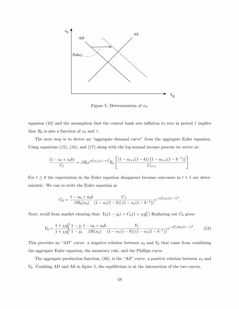
x0

Y0

ADAS

Policy

Figure 5: Determination of x0.

equation (43) and the assumption that the central bank sets inflation to zero in period 1 implies

that R0 is also a function of x0 and τ .

The next step is to derive an “aggregate demand curve” from the aggregate Euler equation.

Using equations (15), (16), and (17) along with the log-normal income process we arrive at:

(1− ut + utb)

Ct= βRte

σ2ε (xt)(1−τ)2Et

[(1− ut+1(1− b))

(1− ut+1(1− b−1)

)Ct+1

].

For t ≥ 0 the expectation in the Euler equation disappears because outcomes in t + 1 are deter-

ministic. We can re-write the Euler equation as

C0 =1− u0 + u0b

βR0(x0)

C1

(1− u1(1− b)) (1− u1(1− b−1))e−σ

2ε (x0)(1−τ)2 .

Next, recall from market clearing that: Y0(1− j0) = C0(1 + χηG0 ) Replacing out C0 gives:

Y0 =1 + χηG01 + χηG1

1− j11− j0

1− u0 + u0b

βR(x0)

Y1

(1− u1(1− b)) (1− u1(1− b−1))e−σ

2ε (M0)(1−τ)2 . (54)

This provides an “AD” curve: a negative relation between x0 and Y0 that came from combining

the aggregate Euler equation, the monetary rule, and the Phillips curve.

The aggregate production function, (36), is the “AS” curve: a positive relation between x0 and

Y0. Combing AD and AS in figure 5, the equilibrium is at the intersection of the two curves.

58

The impact of the social policies on equilibrium slack depends on two features of the diagram.

First, how much does a change in policy horizontally shift the AD curve? A bigger shift in AD will

lead to a larger effect on slack. Second, what are the slopes of the two curves? If both the AD and

the AS are steeper, then a given horizontal shift in the AD brought about by the policies leads to

a larger change in slack at the new equilibrium. We discuss shifts and slopes separately.

E.1 The general equilibrium

Before proceeding, we solve for the intersection of the two curves, the equilibrium of the economy.

First, the AD curve depends on Y1. Under flexible prices, the price-setting first-order condition

implies

w(xt) +ψ1x

ψ2t

h(xt, τ)=ηAtµ.

This equation implies xt is a function of ηAt , τ , and non-policy parameters when prices are flexible.

We call this function xFlex(ηAt , τ). Y1 can be calculated from (36) with x1 = xFlex(ηA1 , τ) because

all prices are flexible in period 1. This leads to

Y1 = ηA1 (1− u(x1)) [w(1− τ)]1

1+γ (x1)ζ

1+γ (55)

Note that x1 is given by xFlex(ηA1 , τ) so (55) makes Y1 independent of x0 and b.

We now set AS = AD. Specifically, equations (54) and (36) lead to two expressions for Y0.

Taking the log of equations (54) and (36) and set them equal to one another yields an implicit

solution for x0:

log

(1− χηG01− χηG1

)+ log(1− j1)− log(1− j0) (56)

+ log (1− u0 + u0b)− log β − log (R(x0, τ)) + log(Y1(xFlex

1 , τ))− log (1− u1(1− b))

− log(1− u1(1− b−1)

)− σ2

ε (x0) (1− τ)2 − log(ηA0)

+ log (S0)− log (h0)− log ((1− u0)) = 0.

E.2 Unemployment benefits and slack

The first result is:

59

Proposition 4. Under the assumptions of section 5.3:

d log x0

d log b= Λ−1

[u0b

1− u0 + u0b+

u1b−1

1− u1(1− b−1)− u1b

1− u1(1− b)

](57)

where Λ is defined below in lemma 3.

Proof. x0 is implicitly defined by (56). Using the implicit function theorem we obtain

dx0

db= −

u01−u0+u0b

− u11−u1(1−b) + u1b−2

1−u1(1−b−1)

− 1−b1−u0+u0b

du0dx0− 1

R0

dR0dx0− (1− τ)2 d

dx0σ2ε (x0) + 1

S0

dS0dx0− 1

h0dh0dx0

+ 11−u0

du0dx0

+ 11−j0

dj0dx0

As an elasticity we have

b

x0

dx0

db=

u0b1−u0+u0b

− u1b1−u1(1−b) + u1b−1

1−u1(1−b−1)

d logR0

d log x0+ (1− τ)2σ2

ε (x0)d log σ2ε (x0)

d log x0+ 1−b

1−u0+u0bu0

d log u0d log x0

− d logS0

d log x0+ d log h0

d log x0+ d log(1−u0)

d log x0+ d log(1−j0)

d log x0

(58)

There are two direct effects of raising unemployment benefits on economic slack. The first

shows the usual logic of the unemployment insurance system as an automatic stabilizer based on

redistribution: aggregate demand responds more strongly to benefits if there are more unemployed

workers. This effect arises because the unemployed have a high marginal propensity to consume so

the extra benefits lead to an increase in demand.

Second, there is an additional effect coming from expected marginal utility in the future, which

depends on the unemployment rate in the next period (t = 1). Expected marginal utility is deter-

mined by two components. The first is the social insurance that UI provides, lowering uncertainty

and precautionary savings and so pushing up aggregate demand today. The second is the higher

taxes in order to finance the higher benefits, which reduce consumption. If the former component

dominates, then the two effects, captured by the expression in square brackets, shift the AD curve

rightwards. As the unemployment rate increases in recessions, both of these effects point towards

a counter-cyclical elasticity.

For the second component to dominate requires that expected marginal utility rises with u1.

For unemployment rates less than 50%, this is true. The proof is as follows: start with u0b1−u0(1−b) ,

60

the derivative with respect to u0 is

b(1− u0(1− b)) + u0b(1− b)[1− u0(1− b)]2

=b

[1− u0(1− b)]2> 0.

Next turn to bu1(1−u1)(b−2−1)[1+u1(b−1−1)][1+u1(b−1)]

. We start by dividing by b(b−2 − 1) ,which is positive for

b ∈ (0, 1). We will then show the derivative with respect to u1 is positive

1− 2u1

[1 + u1(b−1 − 1)] [1 + u1(b− 1)]2[1 + u1(b−1 − 1)

][1 + u1(b− 1)]

− u1(1− u1)

[1 + u1(b−1 − 1)] [1 + u1(b− 1)]2[(b−1 − 1

)(1 + u1(b− 1)) + (b− 1)

(1 + u1(b−1 − 1)

)]> 0

multiply both sides by[

1 + u1(b−1 − 1)]

[1 + u1(b− 1)]2

[1− 2u1][1 + u1(b−1 − 1)

][1 + u1(b− 1)]− u1(1− u1)

[(b−1 − 1

)(1 + u1(b− 1)) + (b− 1)

(1 + u1(b−1 − 1)

)]> 0

Rearranging

(1− 2u1)[1 + (u1 − u2

1)(b−1 + b− 2)]− u1(1− u1)

(b−1 + b− 2

)(1− 2u1) > 0

divide both sides (1− 2u1) (recall u1 < 1/2) and rearrange

1 + u1(1− u1)(b−1 + b− 2)− u1(1− u1)(b−1 + b− 2

)= 1 > 0.

The overall effect on tightness is tempered by the slopes of AD and AS, through the term Λ.

We explain this effect below, but since it is common to the effect of more progressive taxes, we turn

to that first.

E.3 Tax progressivity and slack

The next result is:

Proposition 5. Under the assumptions of section 5.3:

d log x0

d log τ= Λ−1

[2σ2

ε (x0) (1− τ) τ − ∂ logR0

∂ log τ

∣∣∣∣x

+∂ logS0

∂ log τ

∣∣∣∣x

+d log Y1

d log x1

d log x1

d log τ

](59)

61

where Λ is defined below in lemma 3.

Proof. Using the implicit function theorem to differentiate (56) we obtain

dx0

dτ= −

2σ2ε (x0) (1− τ) + 1

Y11

1+γY1

1−τ −1h0

11+γ

h01−τ + 1

S0

∂S0∂τ

∣∣∣x− 1

R0

∂R0∂τ

∣∣∣x

+ 1Y1

dY1dx1

dxFlex(A1,τ)dτ

− 1−b1−u0+u0b

du0dx0− 1

R0

dR0dx0− (1− τ)2 d

dx0σ2ε (x0) + 1

S0

dS0dx0− 1

h0dh0dx0

+ 11−u0

du0dx0

+ 11−j0

dj0dx0

= −2σ2

ε (x0) (1− τ)− 1R0

∂R0∂τ

∣∣∣x

+ 1S0

∂S0∂τ

∣∣∣x

+ 1Y1

dY1dx1

dxFlex(A1,τ)dτ

− 1−b1−u0+u0b

du0dx0− 1

R0

dR0dx0− (1− τ)2 d

dx0σ2ε (x0) + 1

S0

dS0dx0− 1

h0dh0dx0

+ 11−u0

du0dx0

+ 11−j0

dj0dx0

As an elasticity we have

τ

x0

dx0

dτ=

2σ2ε (x0) (1− τ) τ − ∂ logR0

∂ log τ

∣∣∣x

+ ∂ logS0

∂ log τ

∣∣∣x

+ d log Y1d log x1

d log x1d log τ

d logR0

d log x0+ (1− τ)2σ2

ε (x0)d log σ2ε (x0)

d log x0+ 1−b

1−u0+u0bu0

d log u0d log x0

− d logS0

d log x0+ d log h0

d log x0+ d log(1−u0)

d log x0+ d log(1−j0)

d log x0

(60)

The first term in between square brackets reflects the effect of social insurance on aggregate

demand. When households face uninsurable skill risk, a progressive tax system will raise aggregate

demand by reducing the precautionary savings motive. This term will be counter-cyclical if risk

increases in a recession as has been documented by Guvenen et al. (2014).

The remaining terms inside the brackets reflect the effect of a change in τ on marginal cost

holding xt fixed. These terms arise because hiring costs are spread over the hours of the worker so

that even at given levels of wt and Mt, a more progressive tax would lower hours worked per worker

and raise hiring costs per hour worked. If labor supply were fixed on the intensive margin, these

terms would not be present. With a choice of hours of work, we see that higher marginal costs put

upward pressure on prices which is reflected in real interest rates via the monetary policy rule and

in price dispersion. For similar reasons, an increase in τ puts upward pressure on marginal cost in

period 1. As prices are flexible in period 1 this force leads to a reduction in labor market tightness

in period 1 so that marginal cost is again equal to the inverse of the desired markup. Because these

effects all operate through rescaling the hiring costs, which are themselves small, they are not likely

to be important quantitatively.

62

E.4 Slopes of AS and AD

Finally, we turn to Λ, which reflects the slopes of the AS and AD curves. As the previous two

propositions showed, a larger Λ attenuates the effect of the social policies on slack, because it makes

both AS and AD flatter. The next lemma describes what determines it:

Lemma 7. Under the assumptions of section 5.3:

Λ =d logR0

d log x0+ (1− τ)2σ2

ε (x0)d log σ2

ε (x0)

d log x0+

1− b1− u0 + u0b

u0d log u0

d log x0

+d log h0

d log x0+d log(1− u0)

d log x0+d log(1− J0/Y0)

d log x0− d logS0

d log x0(61)

Proof. See (58) and (60).

The first line has the three terms that affect the slope of the AD curve. The first effect involves

the real interest rate. A booming economy leads to higher nominal interest rates, both directly

via the Taylor rule and indirectly via higher inflation. With nominal rigidities, this raises the real

interest rate, which dampens the effectiveness of any policy on equilibrium slack. In other words, a

more aggressive monetary policy rule (or more flexible prices) makes AD flatter and so attenuates

the effectiveness of social policies. An extreme example of this is when the economy is at the zero

lower bound, which magnifies the effectiveness of the automatic stabilizers.34

The second term refers to income risk. If risk is counter-cyclical, this term is negative, so it

makes social programs more powerful in affecting slack. The reason is that there is a destabilizing

precautionary savings motive that amplifies demand shocks. In response to a reduction in aggre-

gate demand, labor market tightness falls, leading to an increase in risk and an increase in the

precautionary savings motive and so a further reduction in aggregate demand. These reinforcing

effects make the AD curve steeper so that social policies become more effective.

The third term reflects the impact of economic expansions on the number of employed house-

holds, who consume more than unemployed households. Therefore, aggregate demand rises as

employment rises in a tighter labor market. This consumption multiplier makes the AD curve

steeper and increases the effectiveness of social programs.

34 McKay and Reis (2016) and Kekre (2017) show that automatic stabilizers and unemployment benefits, respec-tively, have stronger stimulating effects when the economy is at the zero lower bound.

63

The second line in the lemma has the four terms that affect the slope of the AS. Increasing

slack raises hours worked or employment, this makes the AS flatter as output increases by relatively

more, so it raises Λ and attenuates the effect of social programs. This occurs net of hiring costs,

since the fact that they increase with slack works in the opposite direction. Finally, if in a booming

economy the efficiency loss from price dispersion increases, so S increases, then the AS is likewise

steeper and Λ is lower.

F Description of methods for section 6

F.1 Estimated income process

The material in this appendix describes an implementation of the procedure of Guvenen and McKay

(2017).

The income process is as follows: αi,t evolves as in (2). Earnings are given by αi,twt when

employed and zero when unemployed. Notice that here we normalize ht = 1 and subsume all

movements in ht into wt. While this gives a different interpretation to wt it does not affect the

distribution of earnings growth rates apart from a constant term. The innovation distribution is

given by

εi,t+1 ∼ F (ε;xt) =

N(µ1,t, σ1) with prob. P1,

N(µ2,t, σ2) with prob. P2,

N(µ3,t, σ3) with prob. P3

N(µ4,t, σ4) with prob. P4

The tails of F move over time as driven by the latent variable xt such that

µ1,t = µt,

µ2,t = µt + µ2 − xt,

µ3,t = µt + µ3 − xt,

µ4,t = µt.

64

where µt is a normalization such that Ei[expεi,t+1] = 1 in all periods.

The model period is one quarter. The parameters are selected to match the median earnings

growth, the dispersion in the right tail (P90 - P50), and the dispersion in the left-tail (P50-P10) for

one, three, and five year earnings growth rates computed each year using data from 1978 to 2011.

In addition we target the kurtosis of one-year and five year earnings growth rates and the increase

in cross-sectional variance over the life-cycle. The moments are computed from the Social Security

Administration earnings data as reported by Guvenen et al. (2014) and Guvenen et al. (2015).

Our objective function is a weighted sum of the squared difference between the model-implied and

empirical moments.

The estimation procedure simulates quarterly data using the observed job-finding and -separation

rates and then aggregates to annual income and computes these moments. To simulate the income

process, we require time series for xt and wt. We assume that these series are linearly related to

observable labor market indicators (for details see McKay, 2017). Call the weights in these linear

relationships β. We then search over the parameters P , µ, σ, and β subject to the restrictions

P2 = P3 and σ2 = σ3.

Guvenen et al. (2014) emphasize the pro-cyclicality in the skewness of earnings growth rates.

The estimated income process does an excellent job capturing this as shown in the top panel

of figure 6. The estimated β implies a time-series for xt which shifts the tails of the earnings

distribution and gives rise the pro-cyclical skewness shown in figure 6. We regress this time-series

on the unemployment rate and find a coefficient of 16.7.35 The fourth component of the mixture

distribution occurs with very low probability, and in our baseline specification we set it to zero.

This choice is not innocuous, however, because the standard deviation σ4 is estimated to be very

large and this contributes to the high kurtosis of the earnings growth distribution. In particular,

omitting this component leads to a substantially smaller τ as a result of having less risk in the

economy. We prefer to omit this from our baseline calibration because the interpretation of these

high-kurtosis terms is unclear and we are not entirely satisfied with modeling them as permanent

shocks to skill.

The resulting income process that we use in our computations is as follows: The innovation

35 We regress this estimated time series xt on the unemployment rate, which we smooth with an HP filter withsmoothing parameter 100,000. If we call this regression function f , we then proceed with F (ε′; f(u)).

65

1975 1980 1985 1990 1995 2000 2005 2010-0.2

-0.15

-0.1

-0.05

0

0.05

0.1

0.15

0.2Kelley's skewness

Figure 6: Properties of F (ε).66

distribution is given by

εi,t+1 ∼ F (ε;xt) =∼

N(µ1,t, 0.0403) with prob. 0.9855,

N(µ2,t, 0.0966) with prob. 0.00727,

N(µ3,t, 0.0966) with prob. 0.00727

with

µ1,t = µt,

µ2,t = µt + 0.266− 16.73(ut − u∗),

µ3,t = µt − 0.184− 16.73(ut − u∗),

where u∗ is the steady state is unemployment rate in our baseline calibration. The bottom panels

of figure 6 show the density of ε and how it changes with an increase in the unemployment rate.

F.2 Global solution method

As a first step, we need to rewrite the Calvo-pricing first-order condition recursively:

p∗tpt

=Et∑∞

s=tR−1t,s (1− θ)s−t

(ptps

)µ/(1−µ)Ysµ

(ws + ψ1M

ψ2s /hs

)/As

Et∑∞

s=tR−1t,s (1− θ)s−t

(ptps

)1/(1−µ)Ys

.

Define pAt as

pAt = Et∞∑s=t

R−1t,s (1− θ)s−t

(ptps

)µ/(1−µ)

Ysµ(ws + ψ1M

ψ2s /hs

)/As

and pBt as

pBt = Et∞∑s=t

R−1t,s (1− θ)s−t

(ptps

)1/(1−µ)

Ys

such that

p∗tpt

=pAtpBt.

67

pAt and pBt can be rewritten as

pAt = µYt

(wt + ψ1M

ψ2s /hs

)/At + (1− θ)Et

[(Itπt+1

)−1

π−µ/(1−µ)t+1 pAt+1

](62)

pBt = Yt + (1− θ)Et

[(Itπt+1

)−1

π−1/(1−µ)t+1 pBt+1

]. (63)

The procedure we use builds on the method proposed by Maliar and Maliar (2015) and their

application to solving a New Keynesian model. We first describe how we solve the model for a

given grid of aggregate state variables and then describe how we construct the grid.

There are six state variables that evolve according to

Ei[α1−τi,t+1

]= (1− δ)Ei

[α1−τi,t

]Ei[ε1−τi,t+1ut

]+ δ

Ei [logαi,t+1] = (1− δ) [Ei [logαi,t] + Ei [log εi, t+ 1|ut]]

SAt+1 = St

log ηAt+1 = ρA log ηAt + εAt+1

log ηGt+1 = ρG log ηGt + εGt+1

log ηIt+1 = ρI log ηIt + εIt+1,

where SA is the level of price dispersion in the previous period and the ε terms are i.i.d. normal

innovations.

There are five variables that we approximate with complete second-order polynomials in the

state: (1/Ct), pAt , pBt , Jt, and Vt, where Vt is the value of the social welfare function. We use (15)

and (16) to write the Euler equation in terms of Ct and this equation pins down 1/Ct. pAt and pBt

satisfy (62) and (63). Vt satisfies

Vt = Wt + β Et [Vt+1] .

Jt satisfies Jt = ψ1Mψ2t (υ− ut). Abusing language slightly, we will refer to these variables that we

approximate with polynomials as “forward-looking variables.”

The remaining variables in the equilibrium definition can be calculated from the remaining

equations and all of which only involve variables dated t. We call these the “static” variables.

To summarize, let St be the state variables, Xt be the forward-looking variables, and Yt be the

68

static variables. The three blocks of equations are

S ′ = GS(S,X ,Y, ε′)

X = EGX (S,X ,Y,S ′,X ′,Y ′)

Y = GY(S,X )

where GS are the state-transition equations, GX are the forward-looking equations and GY are the

state equations. Let X ≈ F(S,Ω) be the approximated solution for the forward-looking equations

for which we use a complete second-order polynomial with coefficients given by Ω. We then opera-

tionalize the equations as follows: given a value for S, we calculate X = F(S,Ω) and Y = GY(S,X ).

We then take an expectation over ε′ using Gaussian quadrature. For each value of ε′ in the quadra-

ture grid, we compute S ′ = GS(S,X ,Y, ε′), X ′ = F(S ′,Ω) and Y ′ = GY(S ′,X ′). We can now

evaluate GX (S,X ,Y,S ′,X ′,Y ′) for this value of ε′ and looping over all the values in the quadrature

grid we can compute X = EGX (S,X ,Y,S ′,X ′,Y ′). X will differ from the value of X that was

obtained initially from F(S,Ω). We repeat these steps for all the values of S in our grid for the

aggregate state space. We then adjust the coefficients Ω part of the way towards those implied by

the solutions X . We then iterate this procedure to convergence of Ω.

Evaluating some of the equations of the model involves taking integrals against the distribution

of idiosyncratic skill risk εi,t+1 ∼ F (εi,t+1, ut − u∗). We do this using Gaussian quadrature within

each of the components of the mixture distribution. We compute expectations over aggregate

shocks using Gaussian quadrature as well.

We use a two-step procedure to construct the grid on the aggregate state space. We have six

aggregate states so we choose the grid to lie in the region of the aggregate state space that is visited

by simulations of the solution. We create a box of policy parameters [bL, bH ] × [τL, τH ]. For each

of the four corners of this box, we use the procedure of Maliar and Maliar (2015) to construct a

grid and solve the model. This procedure iterates between solving the model and simulating the

solution and constructing a grid in the part of the state space visited by the simulation. This gives

us four grids, which we then merge and eliminate nearby points using the techniques of Maliar

and Maliar (2015). This leaves us with one grid that we use to solve the model when we evaluate

policies. Each of the grids that we construct have 100 points.

69

G Extended model with savings

In the extension with savings, the household’s problem is (we omit aggregate states for simplicity

of notation)

V (a, n) = maxc,a′,h

log c− h1+γ

1 + γ+ β E

[(1− υ)V (a′, 1) + υV S(a′)

]

such that

c+ a′ = Ra+ (n+ (1− n)b)λ (wh+ d)1−τ ,

where for an employed individual h is a choice and for an unemployed worker h should be replaced

by h(a), which is the equilibrium decision rule of employed workers. The value of entering the

period without a match is

V S(a) = maxq

MqV (a, 1) + (1−Mq)V (a, 0)− q1+κ

1 + κ

.

The relevant efficiency conditions are

βRE[(1− υ + υM ′q′)

1

c(a′, 1)+ υ(1−M ′q′) 1

c(a′, 0)

]=

1

c(a, n)

λ (1− τ) (wh+ d)−τ w = c(a, n)h(a)γ

M [V (a, 1)− V (a, 0)] = q(a)κ.

Let Φ(a) be the distribution of households over beginning of period assets (before interest). Let

N(a,M) ≡ 1−υ+υq(a)M be the probability that a worker with assets a is employed. Define H as

aggregate hours worked per employed worker and Q as average search effort. Aggregate quantities,

are then given by

C =

∫c(a, 1)N(a,M) + c(a, 0) [1−N(a,M)] dΦ(a) (64)

H =

∫h(a)N(a,M)dΦ(a)/

∫N(a,M)dΦ(a) (65)

Q =

∫q(a)dΦ(a). (66)

70

Given the definition of H, total labor input is H(1− u).

An equilibrium of the economy can be calculated from a system equations in 14 variables, three

exogenous processes, the solution to the household’s problem, which gives rise to policy rules for

consumption, work effort, and search effort, and the dynamics of the distribution of wealth Φ(a).

The variables are

Ct, ut, Rt, It, πt, Yt, Gt,Ht, wt, St,p∗tpt, Jt,qt,Mt.

And the equations are: (3), (4), (5), (40), (6), (7), (41), (36), (42), (43), (39), (64), (65), (66). The

exogenous processes are ηAt , ηGt , and ηIt .

71