Finance and Economics Discussion SeriesDivisions of Research & Statistics and Monetary Affairs

Federal Reserve Board, Washington, D.C.

Fiscal Policy in the United States: Automatic Stabilizers,Discretionary Fiscal Policy Actions, and the Economy

Glenn Follette and Byron Lutz

2010-43

NOTE: Staff working papers in the Finance and Economics Discussion Series (FEDS) are preliminarymaterials circulated to stimulate discussion and critical comment. The analysis and conclusions set forthare those of the authors and do not indicate concurrence by other members of the research staff or theBoard of Governors. References in publications to the Finance and Economics Discussion Series (other thanacknowledgement) should be cleared with the author(s) to protect the tentative character of these papers.

Finance and Economics Discussion Series Division of Research and Statistics and Monetary Affairs

Federal Reserve Board, Washington, D.C.

Fiscal Policy in the United States: Automatic Stabilizers, Discretionary Fiscal Policy Actions, and the Economy

Glenn Follette and Byron Lutz NOTE: Staff working papers in the Finance and Economics Discussion Series (FEDS) are preliminary materials circulated to stimulate discussion and critical comment. The analysis and conclusions are those of the authors and do not indicate concurrence by other members of the research staff or the Board of Governors. Reference to the Finance and Economics Discussion Series (other than acknowledgement) should be cleared with the author(s) to protect the tentative character of these papers.

Fiscal Policy in the United States: Automatic Stabilizers, Discretionary Fiscal Policy Actions, and the Economy

Glenn Follette and Byron Lutz

June 28, 2010

Abstract

We examine the effects of the economy on the government budget as well as the effects of the budget on the economy. First, we provide measures of the effects of automatic stabilizers on budget outcomes at the federal and state and local levels. For the federal government, the deficit increases about 0.35 percent of GDP for each 1 percentage point deviation of actual GDP relative to potential GDP. For state and local governments, the deficit increases by about 0.1 percent of GDP. We then examine the response of the economy to the automatic stabilizers using the FRB/US model by comparing the response to aggregate demand shocks under two scenarios: with the automatic stabilizers in place and without the automatic stabilizers. Second, we provide measures of discretionary fiscal policy actions at the federal and state and local levels. We find that federal policy actions are somewhat counter-cyclical while state and local policy actions have been somewhat pro-cyclical. Finally, we evaluate the impact of the budget, from both automatic stabilizers and discretionary actions, on economic activity in 2008 and 2009.

JEL classification: E62, H60, H70.

1

Fiscal Policy in the United States: Automatic Stabilizers, Discretionary Fiscal Policy Actions, and the Economy

Glenn Follette and Byron Lutz

Introduction

Fiscal policy has been a key policy tool in addressing the aggregate demand

consequences of the financial crisis in the United States. This paper examines fiscal policy at

both the federal and state and local level and looks at the effects of both automatic stabilizers and

discretionary fiscal actions. Our analysis involves three steps. First, we provide measures of the

effects of the automatic stabilizers on budget outcomes at the federal and state and local levels.

For the federal government, the deficit increases about 0.35 percent of GDP for each 1

percentage point deviation of actual GDP relative to potential GDP. For state and local

governments, the deficit increases by about 0.1 percent of GDP. We then examine the response

of the economy to these automatic stabilizers using the FRB/US model by comparing the

response to aggregate demand shocks under two scenarios: with the automatic stabilizers in place

and without the automatic stabilizers. Second, we provide measures of discretionary fiscal

policy actions at the federal and state and local levels. We find that federal policy actions are

somewhat counter-cyclical: expenditures and tax actions are typically more stimulative after a

business cycle peak than before the peak. In contrast, we find that state and local policy actions

have been somewhat pro-cyclical, probably reflecting constitutional restrictions on general fund

budget balances. We also consider the multiplier impacts of these actions. Third, armed with

the information from our two estimation steps, we evaluate the impact of the budget, from both

automatic stabilizers and discretionary actions, on economic activity over the past two years.

1. Automatic stabilizers

To assess the effect of the business cycle on government budgets, we use a high-

employment budget framework that allows us to separate National Income and Product Accounts

(NIPA) revenues and expenditures into their cyclical and non-cyclical components; our measures

are based on the methodology developed for the federal budget by Frank de Leeuw et al (1980),

refined by Cohen and Follette (2000), and subsequently applied to the state and local sector by

Knight, Kusko, and Rubin (2003), and Follette, Kusko and Lutz (2008). The high-employment

budget methodology allows us to strip out the effects of cyclical macroeconomic developments

2

on actual budget outcomes and thus provides an indication of the path the budget would have

followed had the economy continually operated at its potential level. By design, it is unaffected

by the actions governments take to offset the automatic changes in revenue or expenditures, such

as tax rate increases in response to falling receipts.

To construct our high-employment budget, we use the NIPA budget data at the federal

and state and local levels and the Congressional Budget Office’s (CBO’s) estimates of potential

GDP. Figure 1 shows the estimates of the GDP gap and the difference between the actual

unemployment rate and the NAIRU (which we term “employment slack”). Then we follow the

procedure detailed in Cohen and Follette (2000) to adjust receipts and current expenditures to the

levels they would attain if the economy were operating at its potential level.

The cyclical adjustment to receipts, which accounts for the bulk of the total cyclical

adjustment, depends upon three factors: the composition of receipts, the estimated cyclicality of

the base for each major tax, and the elasticity of the tax to the base.1 For summary statistics we

will report two measures, the elasticity of the overall tax system with respect to cyclical

GDP, / (Table 2), and the change in taxes associated with a 1 percent change in the cyclical

GDP (Table 5). The overall elasticity of the tax system is:

(1) / ∑ ∑ /

where T is total tax collections, Ti is the collection from tax i, Bi is the tax base of tax i, is the

elasticity of Bi with respect to cyclical changes in GDP, is the elasticity of tax i with respect

to Bi and / is the elasticity of tax i with respect to cyclical GDP. Although we estimate time

varying elasticities, the time subscripts are suppressed here for notational simplicity. The second

summary measure, the change in revenues as a percent of GDP, simply equals the product of the

overall elasticity, / , and the tax share of GDP. Accordingly, we require estimates of the

elasticity of tax bases to cyclical changes in GDP, , and elasticities of the taxes to the tax

bases, . The first is accomplished through regressions of components of the tax base with

1 The tax bases for the major taxes are NIPA taxable personal income for personal taxes, NIPA corporate profits for corporate taxes, aggregate wages and salaries for social insurance contributions, NIPA personal consumption expenditures on goods for sales taxes. NIPA taxable personal income is defined as NIPA personal income less transfers plus employee contributions for social insurance. We adjust NIPA corporate profits to remove the earnings of the Federal Reserve System, which are included in the NIPA measure.

3

respect to the GDP gap. The tax elasticities, , are built up from detailed information about the

tax code and its changes over time and a variety of auxiliary regressions.2

Elasticity of the tax bases

Our estimates of the elasticity of the tax bases, , are implemented through several steps

and are based on a few assumptions. First, we assume that each component of the tax base is

potentially differentially affected by cyclical changes in GDP. Second, we assume that the

bases are buffeted by other factors than cyclical changes in GDP, and therefore we do not use

detrending methods, such as an HP filter, to separate trend from cycle because these other factors

would be conflated with the cyclical changes. Third, we assume that the cyclical affects may

appear with some lag. Equation (2) captures these assumptions and equation (3) is the resulting

high-employment tax base.

(2) , . ∑ ,

(3) , ,

For each variable, the “K” denotes the high-employment variable (potential GDP is therefore

denoted as GDPKt), SHAREi is the ratio of the base for tax “i” to GDP, GDPGAP is the

difference between potential GDP and actual GDP divided by potential, BASEi is the relevant

tax base for tax “i”, and lagi quantifies the lag structure for tax i.

We operationalize equation (2) by estimating the first difference of equation 2:

(4) , ∑ , ,

and then using the s to calculate the SHAREKi,t values. We use quarterly data from 1950

through 2008 to estimate the i relationships and the regression results are found in Table 1.3 As

expected, the profit share initially falls as the economy moves into recession while the wage

share rises (see column 1). Figure 2 provides a graphical representation for wages and profits by

plotting the “profits gap” (cyclical profits divided by potential profits) and the “wage gap”

2 We do not attempt to estimate the tax elasticities from the aggregate time series data because movements in taxes in these data also include frequent and sometimes substantial changes in policy. 3 Note, we do not require that the deviations in the shares sum to zero. The deviations in GDI and GDP have a cyclical pattern. Thus, the income gaps do not have to sum to the GDP gap.

4

against the GDP gap. As is clearly visible, wages are nearly perfectly unit elastic, whereas

profits have an elasticity significantly in excess of 1. Finally, in order to display summary

statistics for , we calculate the mean elasticity for each of the major tax bases by regressing

the wage, personal income, and profits gaps on the GDP gap and its lags. These elasticities are

presented in column 2 of Table 2.

Federal government tax elasticities

We now turn to our procedures for estimating the elasticity of taxes to the base, , for

the federal side. These procedures are based on the methodology in Cohen and Follette (2000).

Federal personal income taxes are roughly 45 percent of federal NIPA-based total tax receipts.

Our personal income tax elasticity measure, , reflects two factors: the elasticity of taxes with

respect to the administrative definition of income (called adjusted gross income or AGI) and the

elasticity of AGI with respect to the national accounts measure of income. Furthermore, the

elasticity of income taxes with respect to aggregate AGI is a weighted sum of the number of

returns and average income per return where the weights are the relative contributions of changes

in returns and average income to the cyclical change in income. More formally,

(5) ε ε α ε 1 α ε ε

where ε is the elasticity of taxes with respect to AGI, ε is the elasticity of AGI with

respect to NIPA adjusted personal income, ε is the elasticity of taxes with respect to

changes in the number of returns, and ε which is the elasticity of the income tax schedule

with respect to AGI per return. Finally, α measures the relative importance of the numbers of

returns and income per return in cyclical income.

As detailed in Cohen and Follette (2000) we calculate by taking a weighted average

of separate calculations for single and non-single filers. We assume that ε equals 1 and

construct the weight for single and non-single returns separately by regressing the number of

returns filed and AGI per return to obtain estimates of their relative cyclical sensitivities. We

find that for non-singles α is zero as filing is not cyclically sensitive, but for single filers alpha is

about 0.5. We estimate ε for each year based on that year’s tax schedule and actual

5

distribution of income. Turning to ε , personal income as defined by the tax authorities, AGI,

is more cyclical than personal income in the national accounts (NIPA), perhaps because capital

gains realizations (which are not included in national accounts’ definition of income) appear to

be cyclical. We estimate ε by regressing average AGI per return on NIPA income per

employee, with allowance for a change in the elasticity after the 1986 Tax Reform Act, and find

that the current elasticity is about 1.5, compared to 1.1 before. The resulting estimates for

are shown in Table 2 (columns 3 and 5) (these are mean elasticities, with the mean taken over

time).

The next largest source of revenues for the federal government is social insurance

contributions. These are somewhat inelastic because, while the tax rate is constant the wage base

is capped, and because some sources of social insurance contributions are not based on wages.

The cap, as a fraction of average wages, has fluctuated over time with changes in law and the

distribution of wages. We estimate the elasticity of social insurance contributions, using a

similar methodology used to produce . The resulting estimates are shown in table 2 (columns

3 and 5), with the elasticity rising from about 0.3 in 1965-1985 to 0.7 in 1986-2008 largely as a

result of the wage caps being raised.

The corporate tax system itself is essentially unit elastic as the rate structure is very flat.

As a result, ε is equal to approximately 1.04 and we assume α equals zero. The cyclical

movements in corporate income subject to tax are smaller than those of economic profits because

some adjustments such as loss carry backs are counter-cyclical. We estimate that the elasticity of

corporate income subject to tax with respect to economic profits, ε , is about 0.8. The overall

elasticity of corporate taxes to economic profits, , is therefore about 0.8.

Other taxes—chiefly excise taxes and customs duties—are a small and declining share of

receipts at the federal level. We set the elasticity of customs duties at 2.0, the cyclical elasticity

of imports found in the FRB/US model and the elasticity of excise taxes is built up from demand

elasticities of the various components—many of which, such as tobacco and alcohol—are rather

inelastic. As shown in table 2 the resulting elasticity for these other taxes is around 1.

6

Federal government total tax elasticity and cyclical revenues

Combining the estimates in columns (2) and (3)/(5) of Table 2 allows us to display the

elasticity of the tax receipts with respect to cyclical GDP, / , for the major taxes (see

columns 4 and 6).4 Focusing on the 1986 – 2008 period (column 6), corporate receipts are by far

the most elastic, largely because profits are very elastic (e.g. εB is large). Equation (1) allows

us to pull these estimates together to produce the Federal total tax elasticity, / . For the

earlier period the total elasticity is 1.2 and for the later period it is 1.6. Total federal receipts are

thus currently quite elastic with respect to the business cycle. The elasticity has increased over

time as a result of both the increase in wages subject to social insurance taxes and the 1986 tax

reform’s effect on personal and corporate receipts.

In addition to the revenue elasticities, we also produce analogous estimates of cyclical

revenues: TAXi,t - TAXKi,t (see Table 3 and Figure 3A). These are calculated as

(6) TAXKi,t = TAXi,t + TAXi,t * ((BASEKi,t /BASEi,t) - 1)* ,

where TAXi is tax revenue from tax “i”, TAXKj is the high-employment, or non-cyclical, portion

of tax revenue and BASEKj comes from equation (3). Note that the cyclical revenues are

produced using the time-varying estimates of , and BASEKi,t.

State and local government elasticities and receipts

State and local governments have a less elastic tax system than the federal government

general because they rely more heavily on property taxes and sales taxes which are less

cyclically sensitive and their income tax structures are less elastic. For personal income taxes,

we use the same methodology as at the federal level. However, instead of estimating the

effective elasticity of the tax schedule to IRS-based income, ε , for all of the states, we

assume that it is 1.1. As state income tax systems generally use the same income concept as the

federal government, we use the same estimates made for the federal government for the

sensitivity of IRS income to changes in NIPA personal income, ε . Accordingly, we arrive at

4 We estimate the multiyear elasticities by regressing the log differences of cyclical taxes on the log differences of the cyclical bases (or GDP) which provides the average response over the period with the observed dynamics of the cycle.

7

an overall elasticity of state and local personal income taxes with respect to cyclical personal

income, , of 1.1 before 1986 tax reform, rising to 1.5 afterwards. For corporate income taxes

we use the federal measure of the elasticity of corporate income taxes to NIPA corporate profits

of 0.8. For other taxes, primarily sales and property taxes, we estimate that the cyclical elasticity

is 0.5 as sales taxes are unit elastic and property taxes are inelastic.

In addition to its “own” revenue, state and local governments receive a substantial

amount of federal grants, equal to about 20 percent of their total revenues which are a somewhat

countercyclical revenue source. We cyclically adjust Medicaid and AFDC grants using the

procedure described below for Medicaid expenditures. For other grants from the federal

government, there is no cyclical sensitivity because their levels are set through discretionary

appropriations.

We estimate that the elasticity of total receipts to cyclical GDP, & / , has moved in

the range of ½ to ¾ and have averaged 0.6 over the 1986 to 2008 period (see column 6 of Table

2). The elasticity is well below 1 because property taxes and most federal grants have no or little

cyclical response. The damping effect of grants is substantial as the elasticity of own receipts is

currently about 0.8. The variation over time reflects the changing composition of receipts. Table

3 and figure 3A show our resulting estimates for the cyclical component of state and local

revenues.

Federal Expenditures

Among expenditures, only those transfers and grants that are oriented toward income

support respond automatically to changes in economic activity. Fluctuations in unemployment

benefits account for the vast majority of the cyclical swing in expenditures; also contributing to

the swings are changes in the number of beneficiaries of low-income and disability programs

such as food stamps, earned income credit, welfare (prior to the 1996 reform), and disability

insurance. We use both aggregate macro data and micro studies to create estimates for the

cyclical sensitivity of expenditures.

Unemployment benefits are typically available for up to 26 weeks. Since 1970 the time

period is automatically extended in states with high unemployment. However, the automatic

8

trigger appears to be set at “too high” a level and temporary programs have been enacted during

every recession. Our estimates of the cyclical component of the budget exclude expenditures by

the temporary programs because they are not automatic. Based on these observations we

estimate:

(7) ∆ ∆ ∆ ∆

where UIBEN is regular unemployment benefits excluding the temporary benefit expansions,

WS is NIPA wages and salaries and RU is the total civilian unemployment rate (RU).

These regression results indicate that a 1 percentage point increase in the unemployment

rate would boost benefits by 0.25 percent of wages and salaries over the first two quarters, or

0.10 percent of potential GDP, dropping back a bit in the third quarter as benefit eligibility is

exhausted (see Table 4).

Other changes in expenditures are smaller individually, but sum to about the same total as

unemployment benefits. The food stamp program is the next largest program. Time series

regressions on the aggregate caseload data, similar to equation (7), indicate that a percentage

point increase in the unemployment rate boosts food stamp expenditures by about 0.04 percent of

GDP. For welfare and Medicaid we draw upon on Blank (2001) and model the cyclical portion

of these programs as a function of past changes in the unemployment rate and infer that

Medicaid grants rise by 0.02 percent of GDP per percentage change in the unemployment rate.

In 1996 federal welfare payments were changed to block grants and are no longer sensitive to

economic conditions, previously it would have raised these expenditures by 0.015 percent of

GDP. Finally, studies using micro data have concluded that both the old age (OASI) and

disability (DI) programs are cyclically sensitive – see Kalman, Rupp, and David Stapleton

(2005) and Autor and Duggan (2006)—b ut that the movements are economically negligible in

size.

Adding up all of the above programs, for every percentage point increase in the

unemployment rate cyclical expenditures rise about 0.15 percent of GDP. Using an Okun’s law

relation of a 0.4 percentage point change in the unemployment rate for each 1 percentage point

9

change in real GDP implies a 0.06 percentage point increase in federal expenditures for each

percent change in real GDP (Table 5 and Figure 3B).

State and local expenditures

State and local government expenditures are equal to about 15 percent of GDP, but only

about 3 percent of GDP are in the cyclically sensitive transfers category. For Medicaid

expenditures and welfare caseloads we again draw upon on Blank (2001) to estimate the cyclical

sensitivity. For other transfers , we use the time series NIPA data and regressions similar to

equation (7) to estimate cyclical sensitivities, but the estimated elasticities are small. All in all,

the overall sensitivity of gross state and local expenditures is quite small and lags the business

cycle by about a year and reaches only about 0.04 percent of GDP per percentage point change in

the unemployment rate. With much of that accompanied automatically by federal grants, the

change in expenditures less grants is only 0.02 percent of GDP per 1 percentage point change in

the unemployment rate and 0.01 percent of GDP per one percent change in cyclical GDP.

Cyclical Deficits

Table 5A brings these pieces of the analysis together to provide estimates of the cyclical

budget sensitivities at the federal, state and local and general government levels. Specifically,

we evaluate our revenue and expenditure elasticities using the current values of revenues and

expenditures as a percent of GDP. (For instance, the Federal total tax elasticity with respect to

cyclical GDP on Table 2 is 1.6 and Federal revenues comprise about 19 percent of GDP. Thus,

the change in Federal revenues as a percent of GDP produced by a 1 percent change in cyclical

GDP is 0.30 – see column 1.) We then subtract the expenditure estimates from the revenue

estimates to produce an estimate of cyclical deficits, or net lending (column 3). State and local

cyclical deficits are much smaller than Federal deficits, likely reflecting balanced budget

requirements at the state and local level.

At the general government level (column 3), the deficit is increased about 0.5 percent of

GDP for every 1 percent decline in GDP.5 In the current environment, the deficit is about 3.3

5 This is a considerably larger response than estimated by van den Noord (2000), largely reflecting different assessments of the elasticity of taxable personal income to cyclical GDP.

10

percent of GDP, or $500 billion, larger than it would if the economy had been at full

employment (Table 5B, column 2, and Figure 3C). Total general government net lending was

around $1600 billion in 2009 (Table 5B, column 1), or 11 percent of actual GDP, thus about 30

percent of the 2009 deficit was generated by the automatic stabilizers.

Effect of automatic stabilizers on the economy

We use simulations of the FRB/US model to examine the degree to which the automatic

fiscal stabilizers considered above help or hinder the performance of the broader economy.6 We

simulate the impact of a negative demand shock under two scenarios. In the first simulation the

automatic stabilizers are left on and the economy is subjected to a series of negative aggregate

demand shocks that by construction lower the level of GDP by 1 percent lower for eight quarters.

The federal funds rate is maintained at its baseline value. In the second simulation we turn off

the federal automatic stabilizers by using a counterfactual tax structure in which taxes are

independent of income and transfers are independent of the unemployment rate and we subject

the economy to the same demand shocks used in the first simulation. A comparison of GDP

growth in the first and second simulations provides an estimate of the extent to which the

stabilizers mute negative demand shocks.

As constructed, in the first simulation, real GDP falls 1 percent for eight quarters. In the

second simulation real GDP falls 1.1 percent after four quarters and 1.2 percent after eight

quarters. Thus, after eight quarters the GDP response to a shock is mitigated by about 20

percent. The implicit multiplier—that is the change in GDP divided by the change in the

deficit—grows to about ½ after eight quarters. There are two reasons for the gradual increase in

the buffering. First, in FRB/US the consumption response to lower taxes (and higher

unemployment benefits) is phased in over time—this is a common feature of many estimated

consumption equations. Second, the multiplier effects gradually increase, particularly because

the federal funds rate is fixed in the two simulations. In the current recession, with the

downward adjustment of the federal funds rate limited by the zero bound, monetary policy would

not be able to offset the additional weakness if the automatic stabilizers were not available, but in

6 FRB/US is a large-scale quarterly econometric model of the U.S. economy developed by the staff of the Federal Reserve. See Brayton and Tinsley (1996) for a detailed introduction to the model.

11

most cases in history the absence of automatic stabilizers could have been offset by more

aggressive monetary policy.

2. Discretionary Policy Actions

This section outlines fiscal impetus (FI), our measure of discretionary policy actions.

Fiscal impetus is a bottom-up approach that involves developing a measure of each major type of

budget action—for example, a cut in personal taxes or an increase in real government

consumption—and aggregating them into a single fiscal indicator that quantifies the impulse to

growth in real GDP coming from budget decisions. The weights used for the aggregation are

based on estimates of the direct effects of budgetary actions on the growth of real GDP. For

example, the weight applied to a reduction in personal taxes is based on an estimate of the

increase in aggregate consumer spending induced by the tax cut—that is, the MPC. Thus, fiscal

impetus is model dependent. Our measure is designed to quantify the first-round effects of

policy changes on GDP growth. It does not take account of subsequent multiplier effects. It also

explicitly excludes the effects of cyclical movements in taxes and transfers (i.e. FI captures only

discretionary policy actions). Two key uncertainties in constructing FI are the timing of the

response and the size of the MPCs. In general we time the impetus with the implementation of

the policy, rather than with the enactment. For example, the effect of defense spending occurs

when the purchases are recorded in the NIPA and consumers are assumed to react to tax cuts

when they observe the lower payments. Some studies, such as Auerbach (2003), instead base

the timing on when the policy is enacted. It is our judgment that the empirical literature finds

very little support for quantitatively important announcement effects on aggregate demand.7

Our MPC estimates are consistent with the coefficients in the macroeconomic models used by

the Federal Reserve Board staff.

7 For example, the consumption literature, in general, finds rule of thumb behavior by many consumers but little support for Ricardian behavior. Survey evidence shows little awareness of tax law changes. By contrast, there is some support for anticipatory changes in taxable income to tax law changes: During the early-1990s year-end bonus payments were shifted to lower tax burdens in response to a series of tax increases. Actual labor supply probably did not change much.

12

Federal

Starting with discretionary tax changes, we assume that such changes are permanent

unless they are explicitly designed to be temporary. Our measures of the real demand effects are

based on estimates of the budget effects of the tax law changes deflated by the appropriate

deflator (consumption or investment).8 For personal or social insurance tax cuts we utilize an

MPC of 0.7 and phase it in over two years following the date of implementation. For temporary

tax changes we assume an MPC of 0.25 in the current quarter and 0.05 in the following quarter,

consistent with studies of recent one-time rebates.9 For corporate tax law changes there can be

two effects: the normal income channel as well as the incentive channel. For general corporate

tax cuts we assume an MPC of 0.5. For changes in investment incentives, such as the two recent

partial expensing provisions, we are guided by the results from House and Shapiro (2008) and

Cohen and Cummins (2006) and assume a small effect on investment demand.

Turning to expenditures, all changes in real purchases of goods and services (which

excludes transfers) are considered discretionary because they are controlled by annual

appropriations. These receive a weight of one. We assume an MPC of 1.0 for legislated changes

in transfer payments (except for one-time payments which are treated like temporary tax cuts)

and we exclude the endogenous changes in transfers owing to demographic factors, automatic

cost-of-living adjustments and other economic factors. The higher MPC for transfers than for

taxes reflects the fact that most transfers go to lower-income households, which are more likely

to be liquidity constrained or follow rule-of-thumb behavior than the taxpaying population as a

whole.

Grants to state and local governments, which are considered to be part of Federal FI at

the time they are spent by the state and localities, are problematic because the degree and timing

of the state and local response is not well understood. We assume that the states and localities

spend the funds over the following two years. This is consistent with the flypaper effect, but

8 Our estimates for legislated changes to taxes or transfers come from a variety of sources, including the Congressional Budget Office and the Administration’s budget. We then translate these estimates into the accounting framework of the national income and product account. 9 See, Sahm, Shapiro, and Slemrod (2009), Coronado, Lupton and Sheiner (2005) and Johnson, Parker and Souleles (2004).

13

overstates the response if states and localities react to increased grants by cutting taxes.10 Our

assumptions about the state and local reaction to grants is important only in assigning stimulus

actions to the federal or state and local level. At the general government level FI does not

depend much on the grant assumptions.11

Figure 4A shows our estimates for federal fiscal stimulus. Several observations jump

out. Federal fiscal policy does appear to be countercyclical. Second, the amount of stimulus in

any given year has been limited, with a boost to aggregate demand of about 1 percent of GDP

being near the top. Third, note that the amount of stimulus in 2009 as a result of last year’s

budget actions is not much different than earlier in the decade when demand was boosted by tax

cuts and defense spending increases. The portion of federal fiscal stimulus that owes to

increased grants to the state and local sector is indicated by the distance between the dashed and

solid lines and this amount will be subtracted from state and local actions to determine their

contribution. Table 6 shows federal fiscal impetus around business cycle peaks; it shows the

impulse to growth in real GDP from the Federal sector during the two years up to and including

the peak and during the three years after the peak. In general, federal fiscal policy has been more

stimulative after the peak than before it, thus moderating the economic downturns. The

exception was following the 1990 peak when policy was focused on long-term deficit reduction.

Our measure of fiscal stimulus registers a positive value when fiscal policy is boosting

aggregate demand. Alternatively FI could be measured relative to whether policy is inducing

growth above or below that of potential GDP. In that context, a neutral fiscal stance corresponds

to the impetus to GDP growth that would emanate if each component of taxes and expenditures

were to grow at the rate of potential GDP. In such a case, the impetus from taxes and transfers

would be zero and the impetus from purchases would equal the rate of growth of real potential

GDP times the share of Federal purchases in GDP. Under a neutral fiscal stance, the Federal

government share of GDP would remain constant. For the federal sector neutral FI would be

10 See Knight (2002) and Lutz (2010) for recent studies of the response of state and local governments to changes in grants which find that state and local governments respond to increased grants by cutting taxes. In this case the MPC would be closer to 0.7, the MPC of a tax cut. 11 The impetus we attribute to an increase in federal grants is deducted from our measure of state and local impetus. For instance, if we overestimate the state and local grant spendout rate, we will mechanically underestimate spending from state and local own source revenue. Thus, general government FI is largely unaffected even if states use the grants to fund tax cuts.

14

approximately 0.2 (CBO’s estimate of potential GDP growth is about 2.5 and Federal purchases

are about 8 percent of GDP).

State and Local

Whenever possible, we use direct information to construct our estimates of state and local

“policy” actions—for example, we use figures from the National Association of State Budget

Officers (NASBO) on enacted state revenue changes to estimate changes in state tax policy.

However, we have no such sources for either local taxes or for state or local expenditures; thus,

we have developed NIPA-based measures of policy change that we believe are satisfactory

alternatives. With regard to property taxes, our policy indicator is the ratio of NIPA property tax

receipts to nominal potential GDP, which we dub the effective property tax rate. When this

effective tax rate is constant from one year to the next, policy is defined as being constant.

Movements in the effective tax rate are interpreted as changes in policy; in general, they occur

either because localities make adjustments to their statutory tax rates or because the rate of

increase in average property assessments differs from the rate of overall inflation (as measured

by the GDP price index). Thus, when property values rise rapidly and local governments do not

offset the increases with decreases in the statutory tax rate, we score the change in revenue as a

policy induced tax increase.12

On the expenditure side, we define constant policy for Medicaid as a constant ratio of

outlays (net of federal grants) to potential GDP, and we interpret deviations in this ratio as

changes in policy.13 We use a similar algorithm for other transfers. For purchases of goods and

services, we include both consumption and investment expenditures and define constant policy

as a constant real (i.e. inflation-adjusted) level of purchases. To measure the demand effect of

discretionary changes taxes and transfers, we use the same MPCs as on the Federal side.

As with the federal sector we present two measures of fiscal impetus: with and without

grants. In order to obtain an estimate for general government impetus, the solid line of federal

impetus which includes the impact of grants to the states and localities (Figure 4A) should be

added to the solid state and local line which excludes from impetus the impact of grants from the

12 See Lutz (2009) for a discussion of the response of local governments to changes in real estate prices. 13 We first adjust Medicaid outlays to their high-employment level to remove the cyclical changes from this program.

15

Federal government(Figure 4B). This avoids double counting the effect of grants. As Figure 4B

indicates, state and local fiscal impetus varies a good deal from year to year, but is smaller than

federal actions.

In terms of policy reactions, the middle panel of Table 6 focuses on the behavior of our

state and local fiscal impetus measure around past business cycle peaks. In all six episodes,

policy was expansionary leading up to the peak. During the period following the peak, the

amount of stimulus usually diminished and was only about half as large, on average, as it had

been in period leading up to the peak; the drop-off in fiscal impetus between the two periods

amounted to about 0.2 percent of GDP. This pro-cyclical response probably is the result of state

and local balanced-budget requirements, which while not binding on a year to year basis, do

enforce a significant level of budget discipline.

Discretionary actions

Fiscal impetus is our measure of the direct impact and does not incorporate any crowding

out or crowding in. The total effect on the economy of discretionary actions reflects both the

initial MPC as captured by FI as well as the multiplier (FI does not include multiplier effects and

they therefore must be added to FI in order to obtain the full effect of discretionary actions). The

multiplier depends upon the state of the economy both because of endogenous crowding out and

due to monetary policy responses. The multiplier effects in FRB/US can range from under 1 to

about 2. The multiplier is less than one when both monetary policy is assumed to try to offset

the impetus (such as assuming that it follows a Taylor rule or other such reaction function) and

the fiscal policy is a permanent increase in the deficit, (such as a permanent 1 percent increase

purchases). In this case interest rates rise and the exchange rate appreciates dampening the

demand effect. By contrast, when monetary policy is constrained by the zero bound and if policy

actions are seen as temporary then the multiplier may be as large as 2. As a rule of thumb, a

multiplier of about 1¼ would be generally appropriate if monetary policy is not offsetting fiscal

policy and if the actions are temporary. This multiplier would be applied to FI, not to the

original budget effect. In most discussions of fiscal policy the “multiplier” is a combination of

the MPC and the follow-on effects. Here we address each piece separately.

16

3. The Budget and Economic Activity in 2008-2009

Since the current recession began at the end of 2007 both automatic stabilizers and

discretionary fiscal policy have been at work to buffer the downturn in aggregate demand. In

2008, our measures indicate that policy actions raised real aggregate demand by about 1¼

percent and the automatic stabilizers boosted demand by ¼ percent, on a year-over-year basis.

The increase from discretionary policies in 2008 reflects continued increases in defense

spending, stimulus spending, and other policies. In 2009 discretionary policy actions may have

raised real GDP growth by ¾ percent, including the multiplier effects, and the automatic

stabilizers may have contributed another ½ percentage point. All told, over the two years fiscal

factors (discretionary and automatic) may have lifted the level of GDP by 2¾ percent in 2009.

First, consider the automatic stabilizers. They widened the 2009 deficit by about 3

percent of GDP. FRB/US model simulations indicate that without the stabilizers, output would

have been ¾ percentage point lower on average in 2009. With the deficit 3 percent of GDP

larger and output ¾ percent higher the implicit multiplier is ¼. This is smaller than the figure

derived from the simulation with a constant 1 percent shock. This is because the GDP gap

widened in 2008 and 2009 whereas in the prior experiment it was held constant. Given that the

effects on demand from lower taxes and higher transfers builds over time the implicit multiplier

derived by dividing current quarter change in GDP by the current quarter change in the deficit

will be lower than the value obtained when the shock is constant.

Second, discretionary fiscal policy actions by the federal government boosted aggregate

demand directly by 1 percent in 2008 and another 1 percent in 2009. State and local actions,

excluding those induced by federal grants (which are included in federal FI) had negligible

impact on aggregate demand in 2008, and were contractionary by about -0.4 percent of GDP in

2009. The retrenchment by state and local government largely reflects the pro-cyclical response

induced by balanced budget requirements alluded to above. Combining federal and state and

local discretionary actions together yields 1 percent boost to GDP in 2008 and ½ percent in 2009

leaving real GDP 1½ percent higher in 2009. Applying a multiplier of 1.3 would yield about 2

percent extra GDP in 2009.

17

Considerable attention has been given to the role of the portion of federal discretionary

policies that were explicitly designed to stimulate the economy. During 2008 and 2009

numerous policies were enacted for stimulus reasons, the most prominent being the American

Recovery and Reinvestment Act (ARRA) which passed in February 2009. Other policies

include the 2008 temporary tax cut, the expansion and extension of unemployment benefits that

have occurred several times, aid to first-time home buyers, the 2009 “Cash for Clunkers”

program, and additional corporate tax relief. The Administration has proposed additional

policies for 2010 and 2011, including extending several provisions that are slated to expire this

year. Table 7 reports the significant elements of the enacted measures (including an assumed

further extension of unemployment benefits). Personal tax cuts include a one-time rebate in

2008 and the “Make Work Pay” reduction in income taxes that began in April 2009 and which

we assume will be treated by consumers as a permanent reduction in taxes, although it is slated

to expire after 2010.14 Transfers include increased unemployment benefits that have been part of

five separate bills and which we assume will be extended again through the end of 2010. The

third major piece of stimulus is increased grants to state and local governments for construction,

education and general funds. Minor elements include temporary reductions in corporate taxes

for partial expensing, and provisions to delay payment of taxes for several years through loss-

carry-back and temporary indebtedness relief.

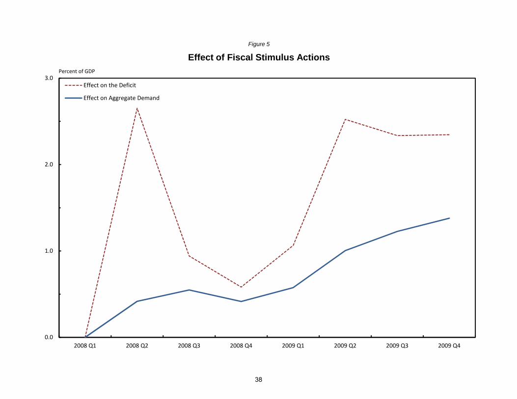
Figure 5 puts these on a national accounts quarterly basis and provides an estimate of

fiscal impetus from stimulus legislation. In our judgment the aggregate demand effects of these

provisions is more muted and drawn out than the budget effects. This reflects several factors. It

is more muted because we assume temporary tax and transfers are mostly saved, particularly the

corporate provisions, but also those for individuals. It is more drawn out because consumers

phase in their response to the permanent tax cuts over several years. Moreover, we assume that

state and local governments are expected to smooth out their spending response to the temporary

boost in grants so that they will not have to make significant adjustments when the grants end at

the end of 2010. Thus, the spending response is spread over the 2009-2012 period rather than

just 2009 and 2010. As a result of these assumptions, the aggregate “MPC” from the stimulus is

well below one in 2009, but eventually cumulates to about 0.7. As shown in Figure 5, the direct

14 We have excluded the temporary extension of AMT relief as is has been provided every years since 2003 and thus it has been previously incorporated in FI.

18

effects of the stimulus actions raise GDP by 1¼ percent by the end of 2009; with a multiplier of

1.3 the total effect is about 1½ percent.15

Conclusions

This paper provides quantitative estimates of the effects of the automatic stabilizers on

the government budget and on the economy. We find that at the general government level each

1 percent increase in the GDP gap increases the deficit by 0.45 percent of GDP with 0.35 percent

of GDP occurring at the federal level. According to simulations with FRB/US, the automatic

stabilizers provide a moderate amount of buffering of aggregate demand shocks. The stabilizers

attenuate the effects on aggregate demand by about 10 percent after four quarters and 20 percent

after eight quarters. Turning to active fiscal policy, the federal government has engaged in

countercyclical policies following most business cycle peaks. This has been offset to some

degree by tightening at the state and local level. During 2008-09, the combined effects of federal

and state and local budgets on aggregate demand (from both discretionary actions and automatic

stabilizers) may have lifted the level of GDP by 2½ percent in 2009.

15 There are a wide range of projections of the effect of the ARRA portion of the stimulus. For example, the Council of Economic Advisors estimates that the year-over-year effect is about 1 percent in 2009 and report that the forecasts from major Wall Street forecasters range from 0.7 to 1.3 percent, with the fourth quarter level ranging from 1½ to 2½ percent.

19

References

Autor and Duggan (2006). “The Rise in Disability Rolls and the Decline in Unemployment,” Journal of Economic Perspectives, Summer 71-96.

Auerbach, Alan J. (2003). “Fiscal Policy, Past and Present,” Brookings Papers on Economic Activity, 1, pp. 75-122.

Aizeman, Joshua and Gurnain Kaur Pasricha (2010). “On the Ease of Overstating the Fiscal Stimulus in the US, 2008-9,” NBER working paper 15784.

Blank, Rebecca (2001). “What Causes Public Assistance Caseloads to Grow?” Journal of Human Resources 36 No. 1 (Winter): 85-118.

Bryaton, F. and P. Tinsley (eds.) (1996). “A Guide to FRB/US: A Macroeconomic Model of the United States” Finance and Economics Discussion Series 1996-42. Washington: Board of Governors of the Federal Reserve System.

Cohen, Darrel (1987). “Models and Measures of Fiscal Policy.” Working Paper Series, Economic Activity Section, No. 70. Washington D.C.: Board of Governors of the Federal Reserve System.

Cohen, Darrel and Jason Cummins (2006). “A Retrospective Evaluation of the Effects of Temporary Partial Expensing,” Finance and Economics Discussion Series, 2006-19. Cohen, Darrel and Glenn Follette (2000). “The Automatic Fiscal Stabilizers: Quietly Doing Their Thing.” Economic Policy Review 6 No. 1 (April): 35-68.

Coronado, Julia, Joseph Lupton and Louise Sheiner (2005). “The Household Spendng Response to the 2003 Tax Cut: Evidence from Survey Data,” Finance and Economics Discussion Series, 2005-32. Council of Economic Advisers (2010). “The Economic Impact of the American Recovery and Reinvestment Act of 2009 Second Quarterly Report,” January 13. deLeeuw, Frank, Thomas Holloway, Darwin Johnson, David McClain, and Charles Waite (1980). “The High-Employment Budget: New Estimates, 1955-1980.” Survey of Current Business (November): 13-43.

Follette, Glenn, Andrea Kusko and Byron Lutz (2008). “State and Local Finances and the Macroeconomy: The High-employment Budget and Fiscal Impetus,” National Tax Journal, September.

20

House, Christopher, and Matthew Shapiro (2008). “Temporary Investment Tax Incentives: Theory with Evidence from Bonus Depreciation,” American Economic Review, September, 1028-1038.

Johnson, David, Jonathan Parker and Nicholas Souleles (2004). “Household Expenditure and the Income Tax Rebates of 2001,” NBER working paper 10784.

Kalman, Rupp, and David Stapleton (1995). “Determinant of the Growth in the Social Security Administration’s Disability Programs—An Overview,” Social Security Bulletin, Winter.

Knight, Brian (2002). “Endogenous Federal Grants and Crowd-out of State Government Spending: Theory and Evidence from the Federal Highway Aid Program,'' American Economic Review, 92(1).

Knight, Brian, Andrea Kusko and Laura Rubin (2003). “Problems and Prospects for State and Local Governments.” State Tax Notes (August 11): 427-439.

Sahm, Claudia R., Mathew D. Shapiro, and Joel Slemrod (2009). "Household Response to the 2008 Tax Rebates: Survey Evidence and Aggregate Implications," Prepared for the NBER Conference on Tax Policy and the Economy Washington, DC (September).

Lutz, Byron (2008). “The Connection Between House Price Appreciation and Property Tax Revenues.” National Tax Journal (September, 2008).

Lutz (2010). "Taxation with Representation: Intergovernmental Grants in A Plebiscite Democracy", Review of Economics and Statistics, forthcoming.

National Association of State Budget Officers (2009). The Fiscal Survey of the States. Washington, D.C. (June).

National Conference of State Legislatures (2008). State Budget Actions FY 2007 and FY 2008. Denver CO. April.

U.S. Congressional Budget Office (2010). “Estimated Impact of the American Recovery and Reinvestment Act on Employment and Economic Output From October 2009 Through December 2009,” February. U.S. Congressional Budget Office (various years). The Budget and Economic Outlook. Washington D.C.

van den Noord, Paul (2000). “The Size and Role of Automatic Fiscal Stabilizers in the 1990s and Beyond”, OECD Economics Department Working Papers, No. 230.

21

Item GDP gapt GDP gapt-1 GDP gapt-2 GDP gapt-3 GDP gapt-4 ∑(GDP gap)

(1) (2) (3) (4) (5) (6)∆ Wages 0.189 -0.121 -0.040 -0.073 0.000 -0.044

t-value 10.072 -6.185 -2.022 -3.736 0.020 n.a.∆ Supplements (inc. employer's) 0.033 -0.004 0.002 -0.012 0.005 0.024

t-value 5.050 -0.621 0.248 -1.743 0.832 n.a.∆ Profits -0.286 0.028 0.069 -0.013 0.107 -0.095

t-value -11.536 1.094 2.678 -0.491 4.278 n.a.∆ Proprietor's income 0.011 -0.003 -0.023 0.001 0.007 -0.007

t-value 0.654 -0.164 -1.344 0.033 0.423 n.a.∆ Rental income 0.021 -0.001 0.008 0.003 -0.005 0.025

t-value 4.019 -0.186 1.441 0.644 -1.016 n.a.∆ Net interest 0.034 0.004 -0.014 -0.017 0.005 0.012

t-value 3.112 -0.186 -1.269 -1.508 0.506 n.a.∆ Rent & net interest 0.054 0.003 -0.007 -0.013 0.000 0.038

t-value 4.536 0.261 -0.529 -1.087 0.021 n.a.∆ HEB property -0.005 -0.002 -0.002 -0.003 0.000 -0.010

t-value -3.209 -1.030 -1.006 -1.669 0.112 n.a.∆ Property 0.466 -0.155 -0.152 -0.245 0.020 -0.065

t-value 3.202 -1.020 -1.007 -1.615 0.137 n.a.∆ Personal consumption, goods 0.066 -0.016 -0.030 0.102 -0.036 0.087

t-value 2.420 -0.550 -1.052 3.568 -1.306 n.a.

Table 1

Share Equations

Note. Dependent variable is the income variable as a share of GDP and then differenced. GDP Gap = (Potential GDP - GDP) / Potential GDP *100

22

NIPA base GDP NIPA base GDP

(1) (2) (3) (4) (5) (6)

EB Eτ Ei / GDP Eτ Ei / GDPFederal

Total (ET / GDP) n.a n.a. 1.2 n.a. 1.6Personal 45% 1.0 1.4 1.4 2.0 2.0Social insurance 37% 1.0 0.3 0.3 0.7 0.7Corporate 14% 4.0 0.7 2.7 0.8 3.7Other taxes 4% 1.0 0.9 0.9 1.0 1.0

State and LocalTotal (ET / GDP) n.a n.a. 0.6 n.a. 0.6

Own revenues 100% n.a n.a. 0.7 n.a. 0.8Personal 24% 1.0 1.1 1.1 1.5 1.5Corporate 4% 4.0 0.7 2.8 0.8 3.6Other taxes 72% 1.0 0.5 0.5 0.5 0.5

Table 2

Tax Elasticities

Note. Estimated elasticities vary from year to year. The table reports multi-year averages.

Elasticity of base

1960-1985 1986-2008Tax elasticityShare of

taxes, 2007

Item

23

Year Federal State & Local Gen. Gov. GDP Gap

(1) (2) (3) (4)

1970 0.10 -0.08 0.02 1.271971 -0.13 -0.07 -0.20 1.051972 0.27 0.08 0.35 -1.141973 0.91 0.26 1.17 -3.591974 -0.12 -0.04 -0.15 0.631975 -1.14 -0.31 -1.45 4.281976 -0.61 -0.15 -0.77 2.271977 -0.22 -0.07 -0.29 0.971978 0.34 0.07 0.40 -0.971979 0.45 0.04 0.50 -0.57

1980 -0.56 -0.17 -0.73 2.251981 -0.84 -0.14 -0.98 1.961982 -1.98 -0.52 -2.50 6.571983 -1.87 -0.41 -2.28 5.181984 -0.65 -0.10 -0.75 1.391985 -0.34 -0.06 -0.40 0.671986 -0.23 -0.05 -0.28 0.571987 -0.31 -0.05 -0.35 0.441988 0.06 0.05 0.11 -0.531989 0.24 0.09 0.33 -1.01

1990 -0.11 -0.01 -0.11 0.121991 -1.16 -0.27 -1.43 3.031992 -1.06 -0.20 -1.26 2.271993 -0.92 -0.17 -1.09 2.071994 -0.51 -0.08 -0.59 0.871995 -0.50 -0.11 -0.61 1.271996 -0.33 -0.07 -0.40 0.611997 0.17 0.05 0.22 -0.611998 0.50 0.14 0.63 -1.561999 0.84 0.25 1.10 -2.87

2000 1.01 0.31 1.33 -3.372001 0.09 0.08 0.17 -0.732002 -0.59 -0.06 -0.65 0.882003 -0.82 -0.11 -0.93 1.452004 -0.40 -0.04 -0.44 0.562005 -0.12 0.00 -0.12 -0.032006 0.00 0.01 0.01 -0.222007 -0.15 -0.03 -0.18 0.192008 -0.66 -0.18 -0.83 2.212009 -2.06 -0.51 -2.57 6.66

Table 3

Cyclical Receipts

Note. GDP Gap = (Potential GDP - GDP) / Potential GDP *100.

(Percent of Potential GDP)

24

Dependent variable RU RU(T-1) RU(T-2)

(1) (2) (3)

UI benefits / Wages*100 0.20 0.06 -0.02t-value (10.40) (2.60) (1.20)

Food Stamps / GDP*100 0.037t-value (4.73)

Independent variables

Table 4

Cyclical Sensitivity of Unemploymentand Food Stamp Benefits

Note. Data are in first differences.

25

Item Own revenuesExpenditures less grants received

Net lending

(1) (2) (3)

General government -0.37 0.09 -0.46

Federal government -0.31 0.08 -0.39

State and local governments -0.06 0.01 -0.07

General government -2.6 0.5 -3.1

Federal government -2.1 0.4 -2.5

State and local governments -0.5 0.1 -0.6

General government -402 72 -474

Federal government -320 62 -381

State and local governments -82 10 -93

Percent of GDP (per one percent change in cyclical GDP)

Percent of potential GDP using CBO's Estimate of Potential GDP in 2009

Billions of dollars using CBO's Estimate of Potential GDP in 2009

Note. The CBO estimated potential GDP in 2009 to be 15,275 billion dollars and the GDP gap to be 6.75%.

Table 5A

Cyclical Response of Budget

26

Item Actual Cyclical High-employment

(1) (2) (3)

General government ‐1579 ‐474 ‐1105Federal government ‐1451 ‐381 ‐1070State and local governments ‐128 ‐93 ‐35

General government ‐11.1 ‐3.3 ‐7.7Federal government ‐10.2 ‐2.7 ‐7.5State and local governments ‐0.9 ‐0.7 ‐0.2

Table 5B

Cyclical Response of Budget

Net lending, 2009 (billions of dollars)

Net lending, 2009 (percent of actual GDP)

Note. The CBO estimated potential GDP in 2009 to be 15,275 billion dollars and the GDP gap to be 6.75%.

27

Peak year 1969 1973 1980 1990 2000 2007 Average

(1) (2) (3) (4) (5) (6) (7)

Federal Government

Year before peak 0.02 0.55 0.19 -0.23 0.30 0.33 0.20Peak -0.77 -0.16 -0.04 -0.27 0.07 0.16 -0.17

1 year after -0.01 0.00 -0.31 -0.47 0.48 0.84 0.092 years after -0.20 0.58 0.76 -0.31 0.95 1.02 0.473 years after 0.55 0.36 0.95 -0.56 0.90 n.a. 0.44

Before -0.38 0.20 0.07 -0.25 0.19 0.24 0.01After 0.11 0.31 0.47 -0.44 0.78 0.93 0.36

State and Local Government

Year before peak 0.89 -0.04 0.31 0.47 0.53 0.06 0.37Peak 0.50 -0.04 0.17 0.52 0.38 0.27 0.30

1 year after 0.21 0.55 -0.21 0.24 0.55 0.04 0.232 years after 0.34 0.48 0.16 0.17 0.35 -0.39 0.183 years after -0.04 -0.05 0.22 0.34 -0.19 n.a. 0.06

Before 0.69 -0.04 0.24 0.50 0.46 0.16 0.33After 0.17 0.33 0.06 0.25 0.24 -0.17 0.15

General Government

Before 0.31 0.16 0.31 0.25 0.65 0.41 0.35After 0.29 0.64 0.52 -0.19 1.01 0.76 0.50

Fiscal Impetus Around Business Cycles

Table 6

(Percent of GDP)

28

2008 2009 2010 2011

(1) (2) (3) (4) (5)

Enacted 845 146 298 324 76

Individual tax cuts* 298 96 81 104 16Expanded UI and other transfers 144 8 80 50 6Aid to state and local governments 202 0 71 97 34Corporate and other tax cuts 117 42 49 32 -6Other spending 85 0 18 41 26

Proposed 271 0 0 133 138

Total 1116 146 298 457 214

Calendar year

Recent Federal Fiscal Stimulus Actions

Table 7

4-year total

* Excludes AMT relief, includes refundable credits.

(Billions of Dollars)

29

2.0

4.0

6.0

8.0GDP Gap

Employment Slack

Figure 1

Estimates of GDP Gap and Employment SlackPercent, Calendar Years

‐6.0

‐4.0

‐2.0

0.0

1950 1955 1960 1965 1970 1975 1980 1985 1990 1995 2000 2005

Note. GDPGAP = (Potential GDP- GDP) / Potential GDP *100. Employment slack is unemployment rate minus NAIRU.

30

0 0

5.0

10.0

15.0

20.0

25.0GDP Gap

Wage Gap

Profit Gap

Figure 2

Estimates of GDP, Wage, and Profit GapsPercent of potential GDP, Calendar Years

‐20.0

‐15.0

‐10.0

‐5.0

0.0

1950 1955 1960 1965 1970 1975 1980 1985 1990 1995 2000 2005

Note. A positive GDP gap implies actual GDP is less than potential GDP.

31

2.0

4.0

6.0

8.0General Government

Federal Government

State & Local Governments

GDP Gap

Figure 3A

Estimates of Cyclical Receipts by GovernmentPercent of Potential GDP

‐6.0

‐4.0

‐2.0

0.0

1970 1975 1980 1985 1990 1995 2000 2005

Note. A positive GDP gap implies actual GDP is less than potential GDP.

32

2.0

4.0

6.0

8.0General Government

Federal Government

State & Local Governments

GDP Gap

Figure 3B

Estimates of Cyclical Expenditures by Government

Percent of Potential GDP

‐6.0

‐4.0

‐2.0

0.0

1970 1975 1980 1985 1990 1995 2000 2005

Note. A positive GDP gap implies actual GDP is less than potential GDP.

33

2.0

4.0

6.0

8.0General Government

Federal Government

State & Local Governments

GDP Gap

Figure 3C

Estimates of Cyclical Deficits by Government

Percent of Potential GDP

‐6.0

‐4.0

‐2.0

0.0

1970 1975 1980 1985 1990 1995 2000 2005

Note. A positive GDP gap implies actual GDP is less than potential GDP.

34

1.0

2.0Fiscal Impetus Including S&L Response to Federal Grants

Fiscal Impetus Excluding S&L Response to Federal Grants

Figure 4A

Estimates of Fiscal Impetus, Federal GovernmentPercent of Real GDP

‐1.0

0.0

1970 1975 1980 1985 1990 1995 2000 2005

35

1.0

2.0Fiscal Impetus Excluding S&L Response to Federal Grants

Fiscal Impetus Including S&L Response to Federal Grants

Figure 4B

Estimates of Fiscal Impetus, State and Local GovernmentsPercent of Real GDP

‐1.0

0.0

1970 1975 1980 1985 1990 1995 2000 2005

36

1.0

2.0

Figure 4C

Estimates of Fiscal Impetus, General GovernmentPercent of Real GDP

‐1.0

0.0

1970 1975 1980 1985 1990 1995 2000 2005

37

2.0

3.0Effect on the Deficit

Effect on Aggregate Demand

Figure 5

Effect of Fiscal Stimulus ActionsPercent of GDP

0.0

1.0

2008 Q1 2008 Q2 2008 Q3 2008 Q4 2009 Q1 2009 Q2 2009 Q3 2009 Q4

38