Optical properties of colloidal systems

Optical properties of colloidal systems

Rubén G. Barrera*Instituto de Física, UNAM

Mexico

Rubén G. Barrera*Instituto de Física, UNAM

MexicoTonanzintla, 2006

* Consultant at Centro de Investigación en Polímeros, Grupo Comex

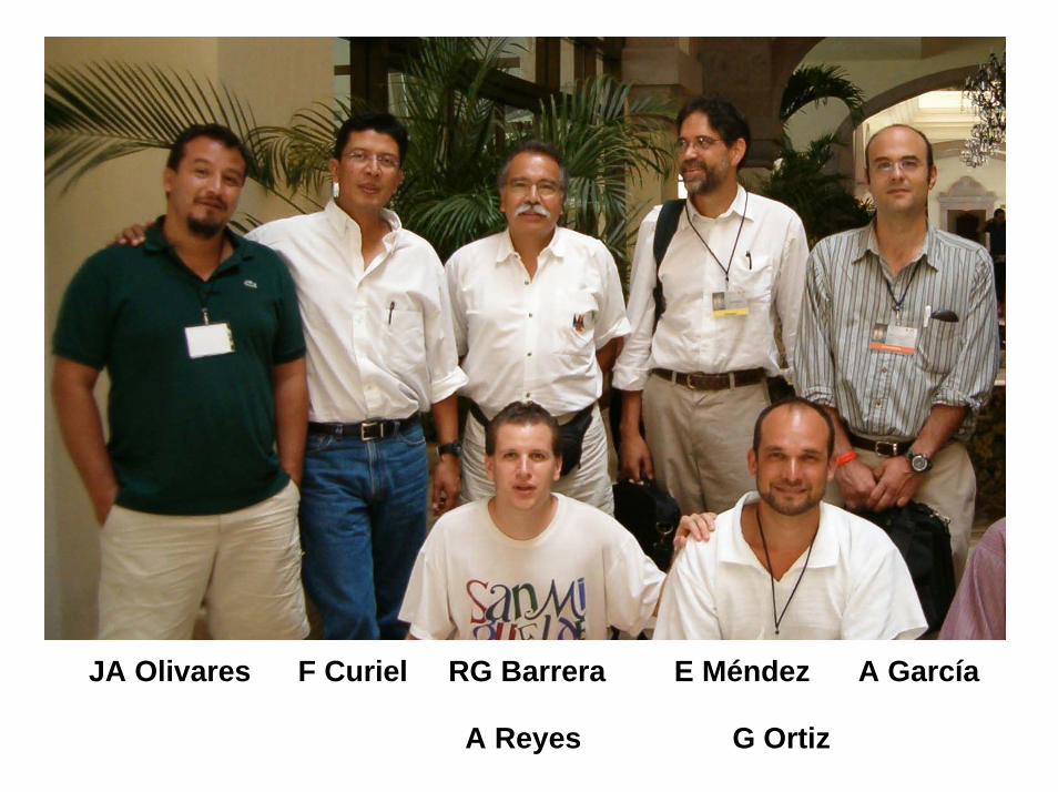
JA Olivares F Curiel RG Barrera E Méndez A García

A Reyes G Ortiz

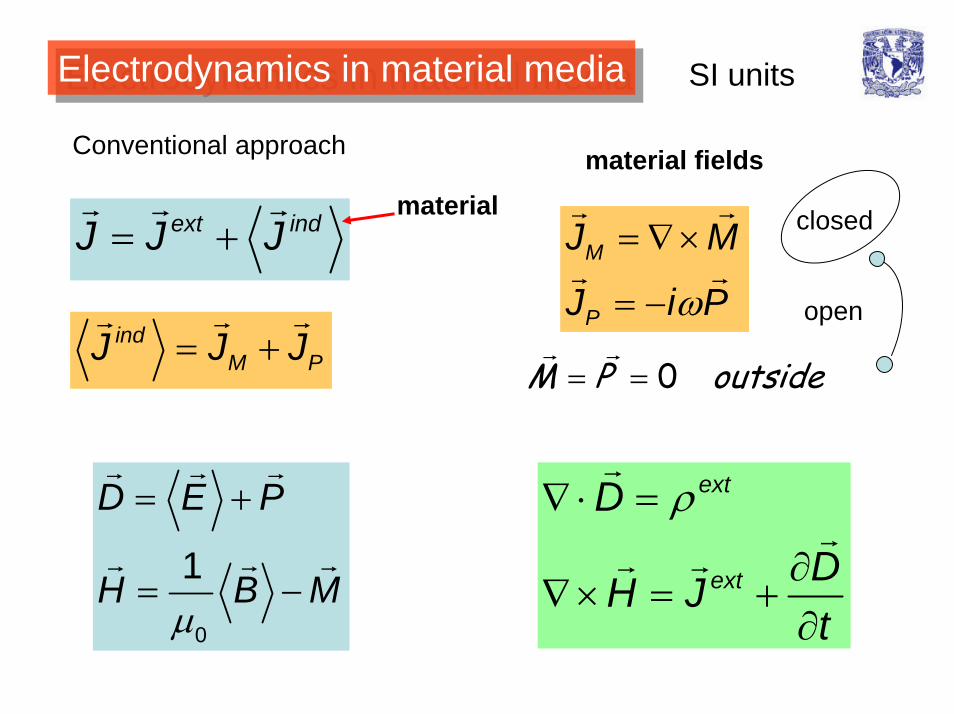
Electrodynamics in material mediaElectrodynamics in material media SI units

Conventional approach

ω

= ∇×

= −M

P

J M

J i P

material fields

closed

open

0M P outside= =

= +ext indJ J Jmaterial

= +indM PJ J J

ρ∇ ⋅ =

∂∇× = +

∂

ext

ext

D

DH Jtµ

= +

= −0

1

D E P

H B M

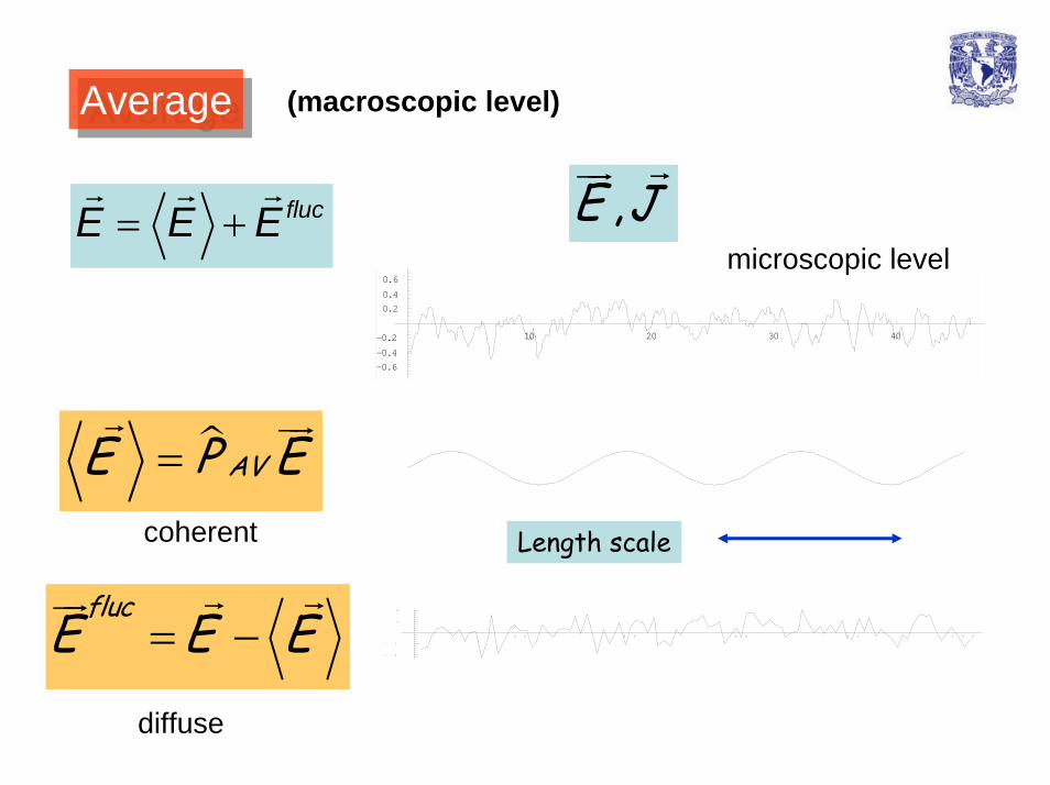
AverageAverage (macroscopic level)

,E J= + flucE E E

10 20 30 40

-0.6-0.4

-0.2

0.20.4

0.6microscopic level

= AVE P Ecoherent Length scale

= −flucE E E 2 0 4 0 6 0 8 0 1 0 0

- 2

- 1

1

2

diffuse

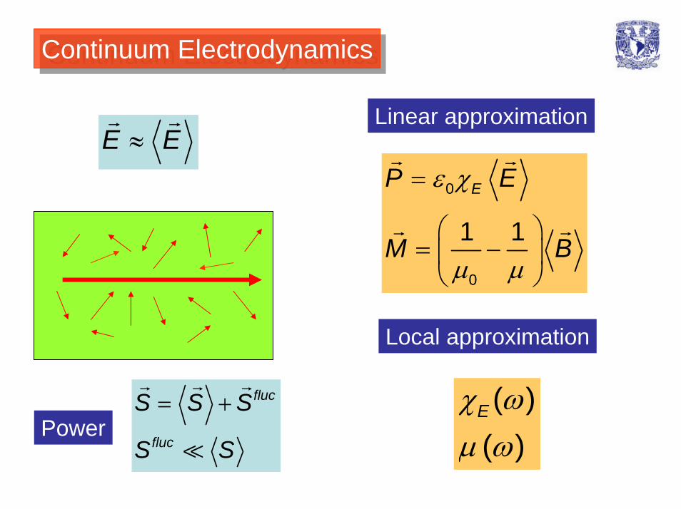
Continuum ElectrodynamicsContinuum Electrodynamics

Linear approximation≈E E

ε χ

µ µ

=

⎛ ⎞= −⎜ ⎟⎝ ⎠

0

0

1 1

EP E

M B

Local approximation

= + fluc

fluc

S S S

S S

χ ωµ ω

( )( )E

Power

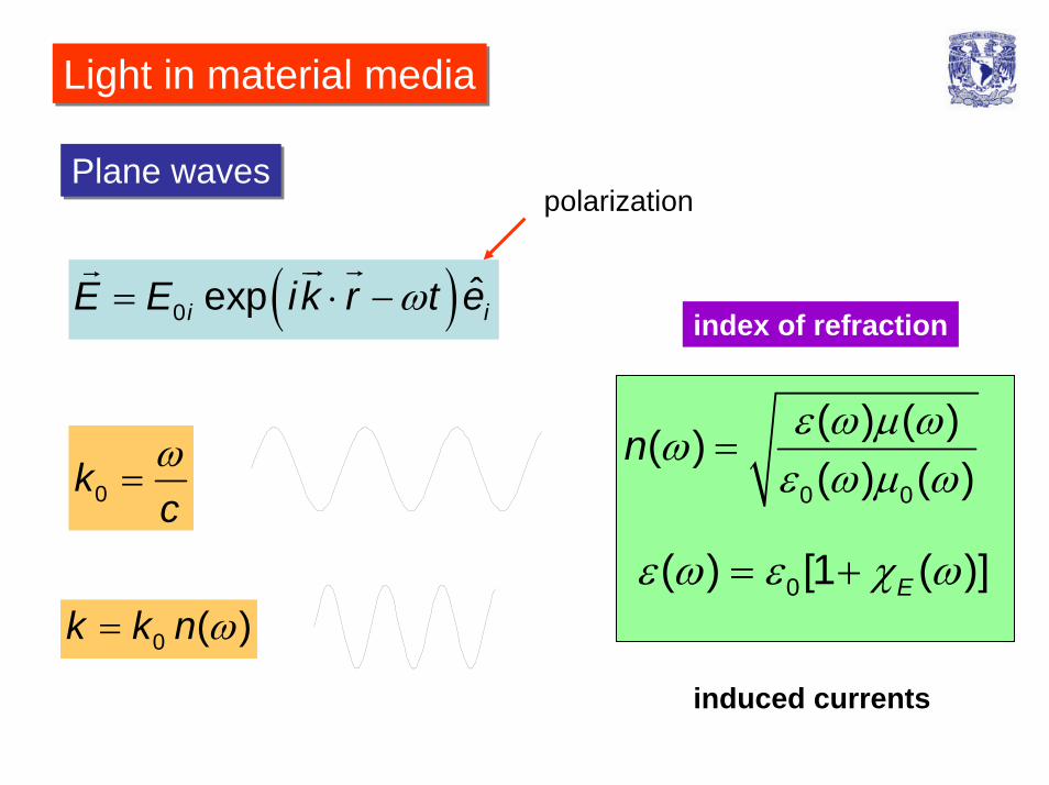
Light in material mediaLight in material media

Plane wavesPlane wavespolarization

( )ω= ⋅ −0 ˆexpi iE E ik r t eindex of refraction

ε ω µ ωωε ω µ ω

=0 0

( ) ( )( )( ) ( )

nω=0k

cε ω ε χ ω= +0( ) [1 ( )]E

ω= 0 ( )k k n

induced currents

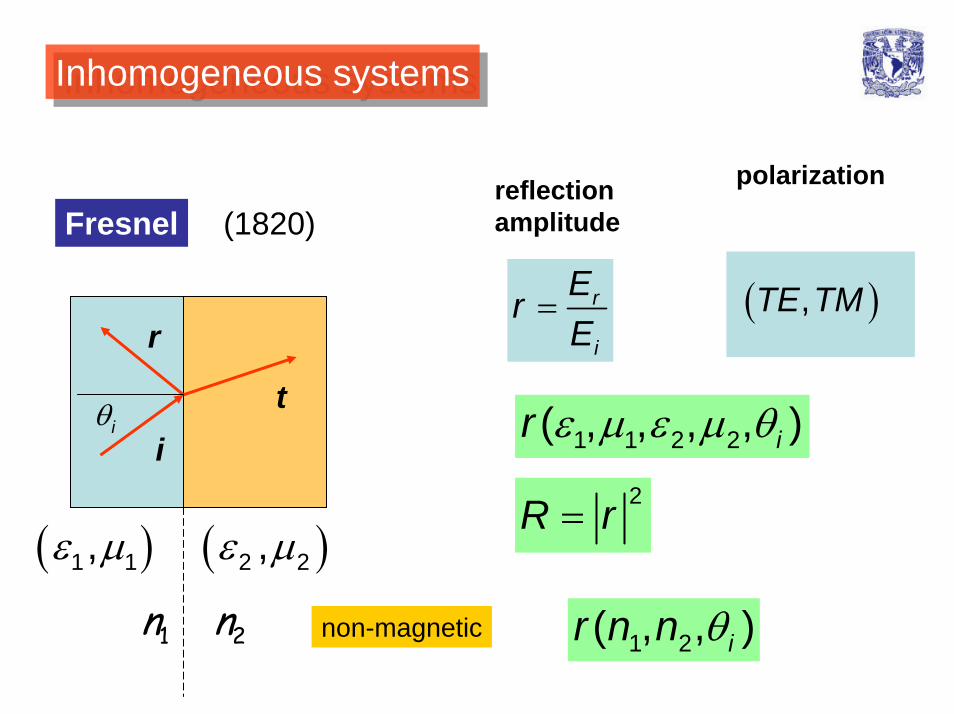
Inhomogeneous systemsInhomogeneous systems

Fresnel

( )ε µ1 1,

i

r

tθi

( )ε µ2 2,

= r

i

ErE

( ),TE TM

reflectionamplitude

polarization

ε µ ε µ θ1 1 2 2( , , , , )ir

(1820)

=2R r

non-magnetic1 2n n θ1 2( , , )ir n n

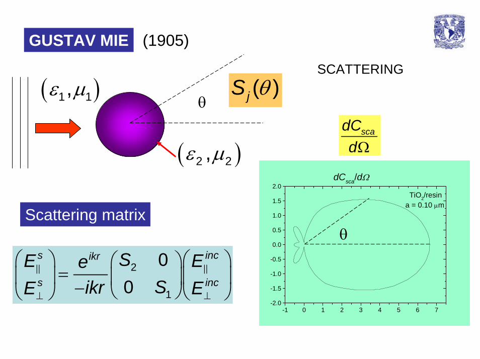
GUSTAV MIE (1905)

⊥ ⊥

⎛ ⎞ ⎛ ⎞⎛ ⎞=⎜ ⎟ ⎜ ⎟⎜ ⎟− ⎝ ⎠⎝ ⎠ ⎝ ⎠

2

1

00

s incikr

s inc

SE EeSikrE E

Scattering matrix

θθ( )jS( )ε µ1 1,

( )ε µ2 2,

-1 0 1 2 3 4 5 6 7-2.0

-1.5

-1.0

-0.5

0.0

0.5

1.0

1.5

2.0 TiO2/resina = 0.10 µm

dCsca/dΩ

ΩscadC

d

θ

SCATTERING

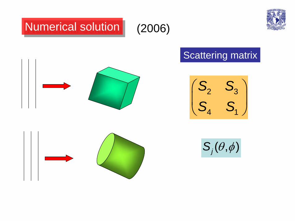
Numerical solutionNumerical solution (2006)

Scattering matrix

⎛ ⎞⎜ ⎟⎝ ⎠

2 3

4 1

S SS S

θ φ( , )jS

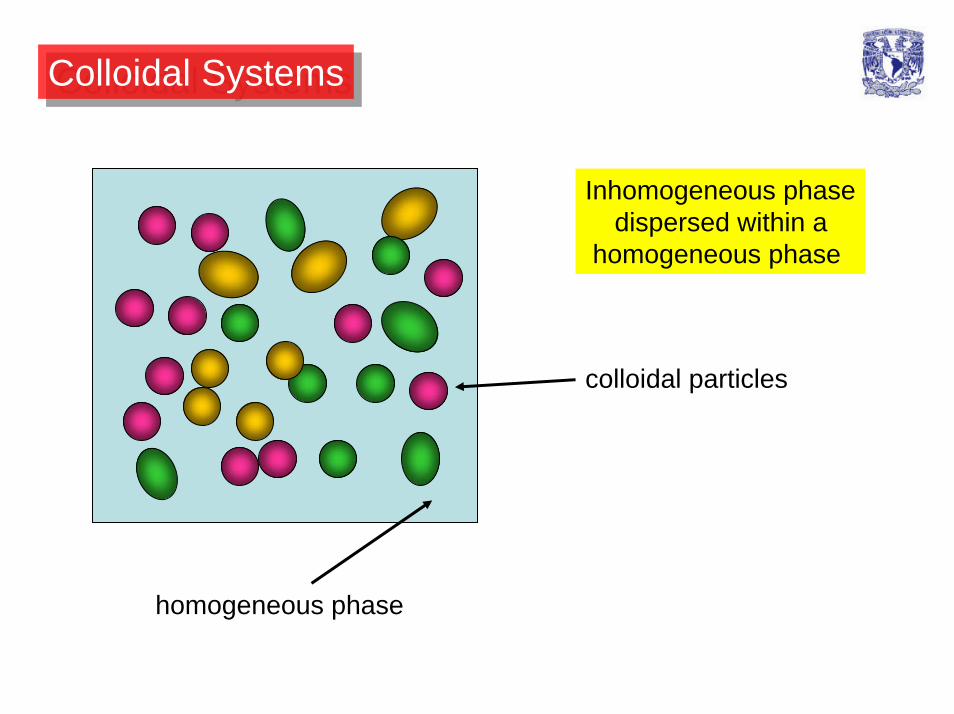
Colloidal SystemsColloidal Systems

Inhomogeneous phasedispersed within a

homogeneous phase

colloidal particles

homogeneous phase

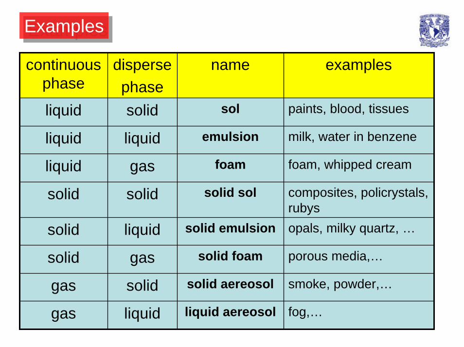
ExamplesExamples

continuousphase

dispersephase

name examples

liquid solid sol paints, blood, tissues

liquid liquid emulsion milk, water in benzene

liquid gas foam foam, whipped cream

solid solid solid sol composites, policrystals, rubys

solid liquid solid emulsion opals, milky quartz, …

solid gas solid foam porous media,…

gas solid solid aereosol smoke, powder,…

gas liquid liquid aereosol fog,…

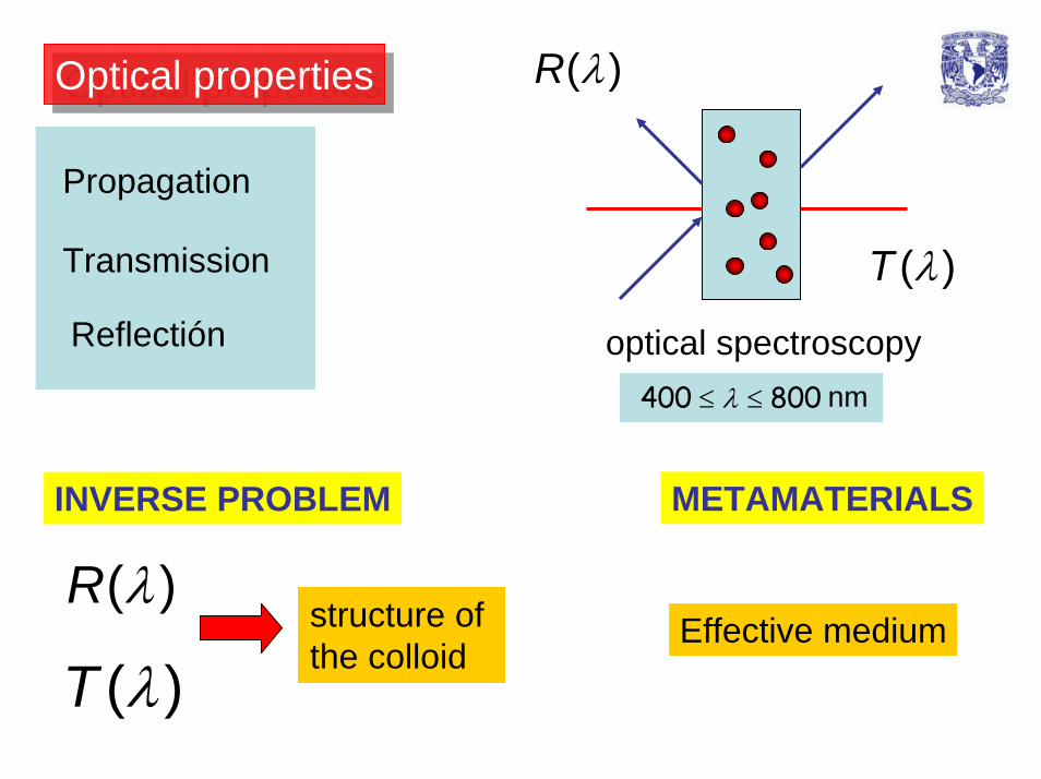
Optical propertiesOptical properties ( )R λ

( )T λ

Propagation

Transmission

Reflectión optical spectroscopy400 800λ≤ ≤ nm

METAMATERIALSINVERSE PROBLEM

( )R λ

( )T λstructure of the colloid

Effective medium

ExampleExample reflectionspectroscopyreflection

spectroscopy

critical angle

milk1 1.50n =

2n2

1

sin cnn

θ =

effective index of refraction

2nδ state of aggregationparticle sizing

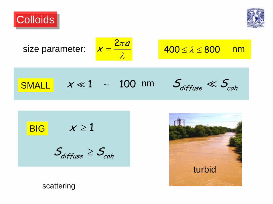
ColloidsColloids

2 ax πλ

=size parameter: 400 800λ≤ ≤ nm

SMALL 1 100x ∼ nm diffuse cohS S

BIG 1x ≥

diffuse cohS S≥

turbid

scattering

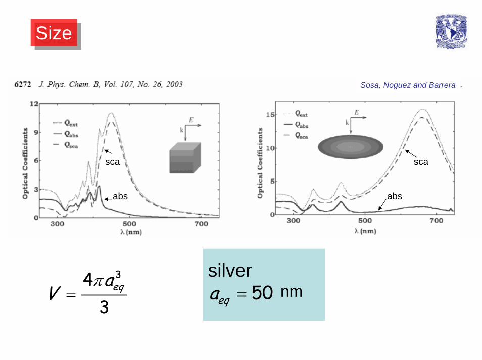
SizeSize

Sosa, Noguez and Barrera

sca sca

absabs

50eqa =silver

nm34

3eqa

Vπ

=

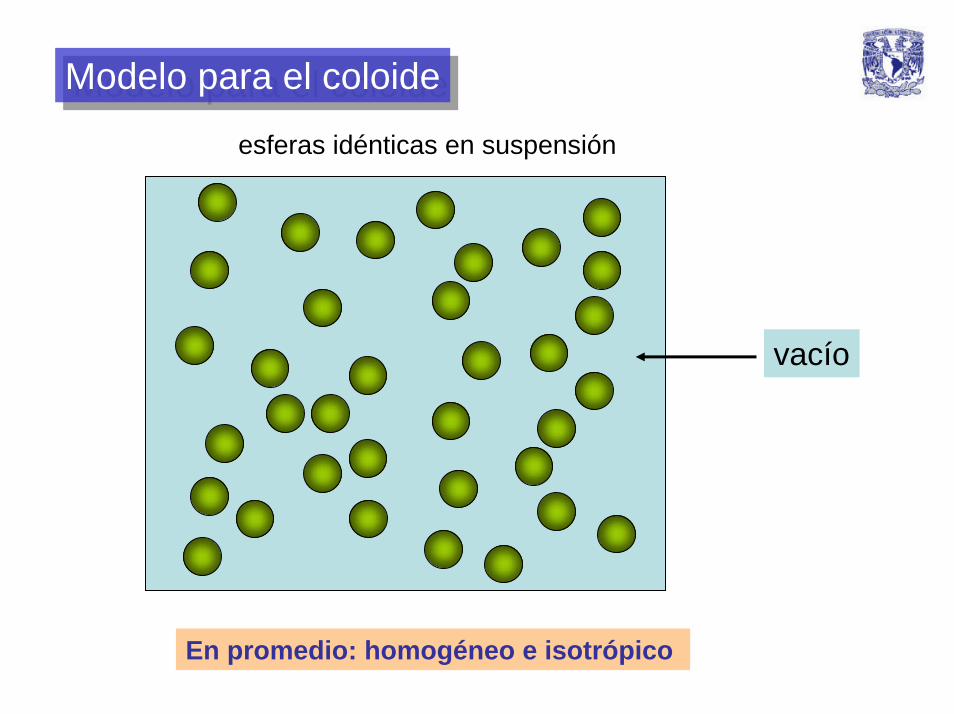
Modelo para el coloideModelo para el coloide

esferas idénticas en suspensión

vacío

En promedio: homogéneo e isotrópico

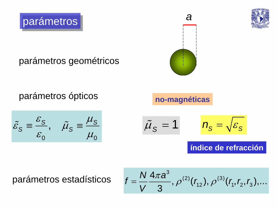
aparámetrosparámetros

parámetros geométricos

parámetros ópticos no-magnéticas

0 0

,S SS S

ε µε µ

ε µ≡ ≡ S Sn ε=1Sµ =

índice de refracción

3(2) (3)

12 1 2 34 , ( ), ( , , ),...

3N af r r r rV

π ρ ρ=parámetros estadísticos

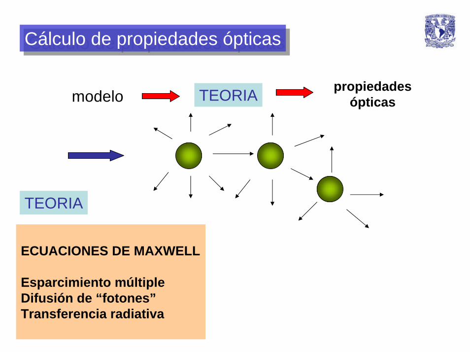
Cálculo de propiedades ópticasCálculo de propiedades ópticas

propiedadesópticasTEORIAmodelo

TEORIA

ECUACIONES DE MAXWELL

Esparcimiento múltipleDifusión de “fotones”Transferencia radiativa

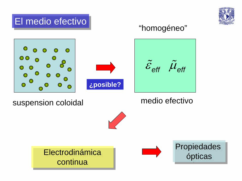
El medio efectivoEl medio efectivo“homogéneo”

eff effε µ¿posible?

medio efectivosuspension coloidal

Propiedadesópticas

PropiedadesópticasElectrodinámica

continuaElectrodinámica

continua

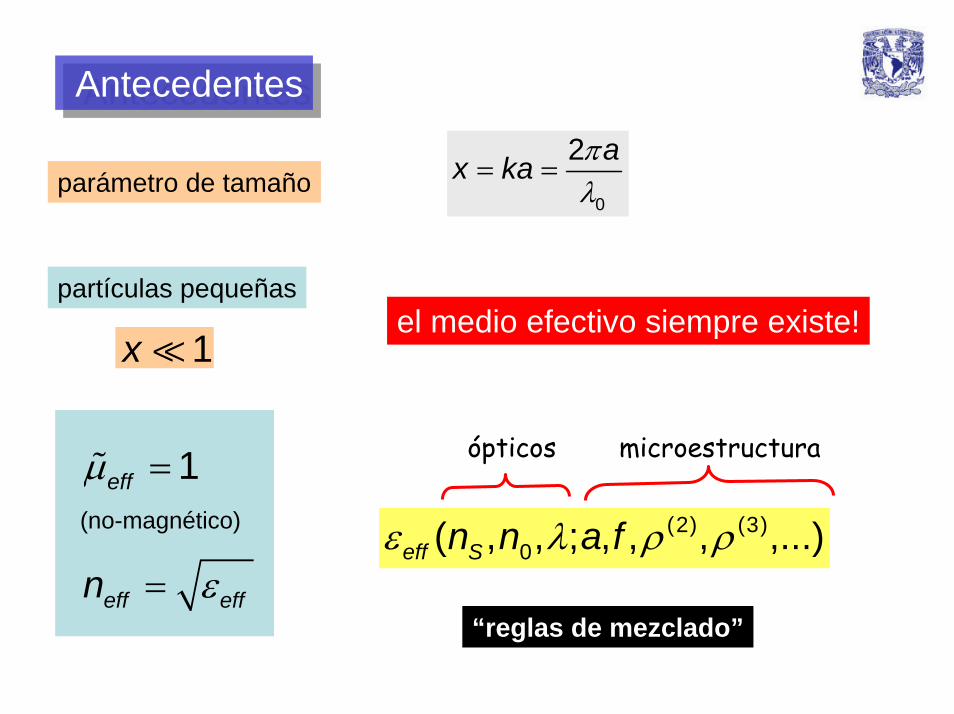
AntecedentesAntecedentes

0

2 ax ka πλ

= =parámetro de tamaño

partículas pequeñasel medio efectivo siempre existe!

1x

ópticos1effµ = microestructura

eff effn ε=

(no-magnético) (2) (3)0( , , ; , , , ,...)eff Sn n a fε λ ρ ρ

“reglas de mezclado”

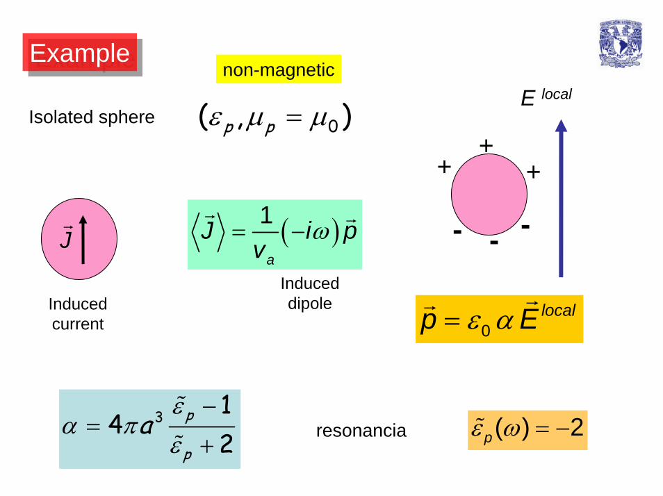
ExampleExamplenon-magnetic

E local

0( , )p pε µ µ=Isolated sphere

( )ω= −1

a

J i pv

++

+

- - -J

Induceddipole

ε α= 0localp E

Inducedcurrent

3 14

2p

pa

εα π

ε−

=+

ε ω = −( ) 2presonancia

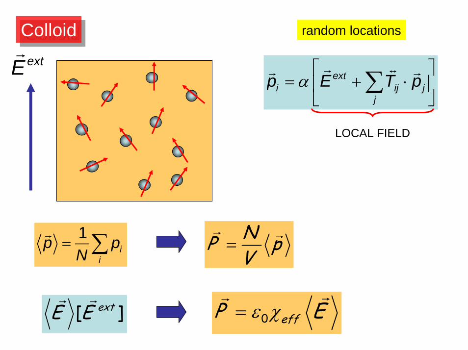
extEColloidColloid random locations

exti ij j

jp E T pα

⎡ ⎤= + ⋅⎢ ⎥

⎣ ⎦∑

LOCAL FIELD

NP pV

== ∑1i

ip p

N

0 effP Eε χ=[ ]extE E

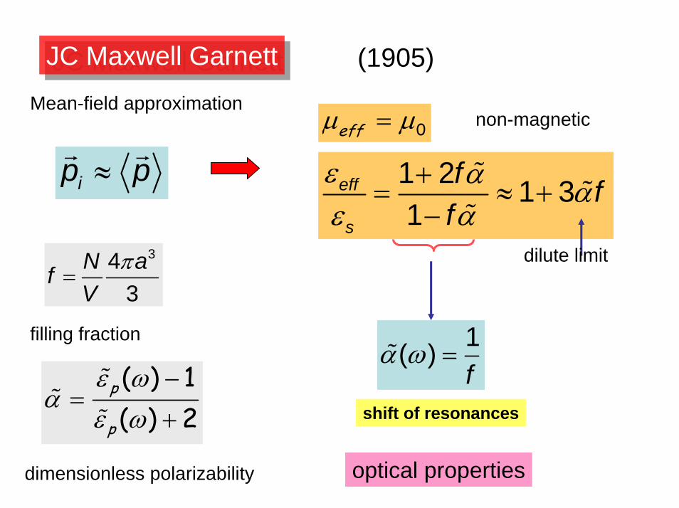
JC Maxwell GarnettJC Maxwell Garnett (1905)Mean-field approximation

0effµ µ= non-magnetic

ip p≈ 1 2 1 31

eff

s

f ff

ε α αε α

+= ≈ +

−

α ω =1( )f

dilute limit343

N afV

π=

filling fraction

( ) 1( ) 2

p

p

ε ωα

ε ω−

=+ shift of resonances

optical propertiesdimensionless polarizability

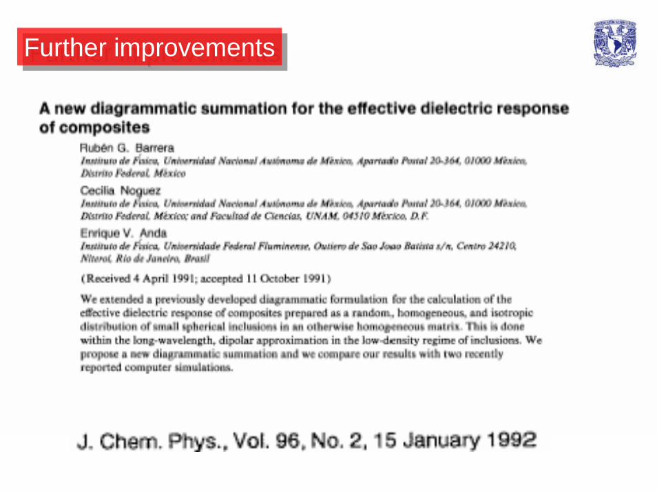
Further improvementsFurther improvements

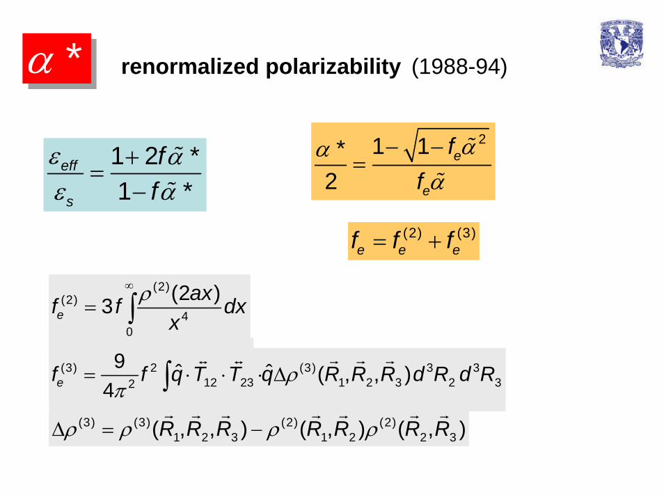
*α renormalized polarizability (1988-94)

21 1*2

e

e

ff

ααα

− −=1 2 *

1 *eff

s

ff

ε αε α

+=

−(2) (3)

e e ef f f= +

(2)(2)

40

(2 )3eaxf f dx

xρ∞

= ∫

(3) 2 (3) 3 312 23 1 2 3 2 32

9 ˆ ˆ ( , , )4ef f q T T q R R R d R d Rρπ

= ⋅ ⋅ ⋅ ∆∫(3) (3) (2) (2)

1 2 3 1 2 2 3( , , ) ( , ) ( , )R R R R R R Rρ ρ ρ ρ∆ = −

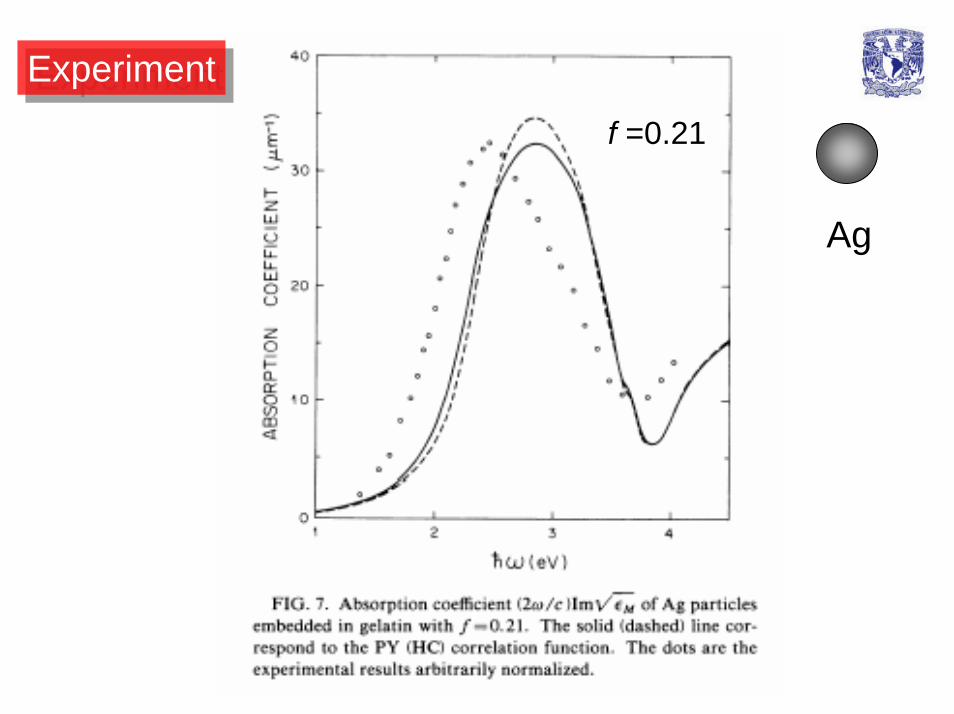
f =0.21

ExperimentExperiment

Ag

Further improvementsFurther improvements

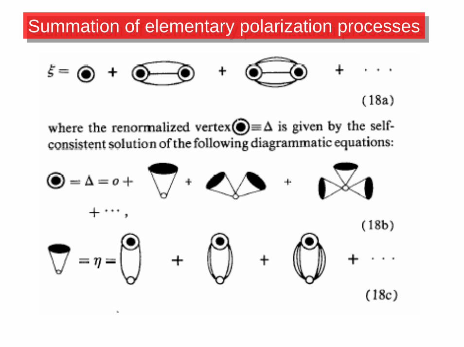
Summation of elementary polarization processesSummation of elementary polarization processes

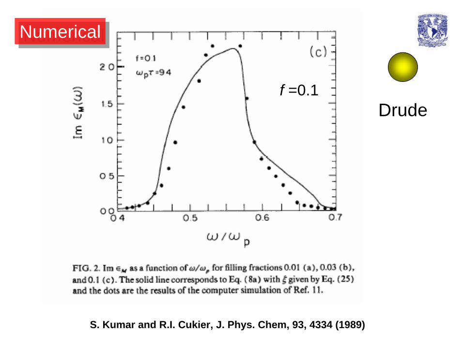
NumericalNumerical

f =0.1Drude

S. Kumar and R.I. Cukier, J. Phys. Chem, 93, 4334 (1989)

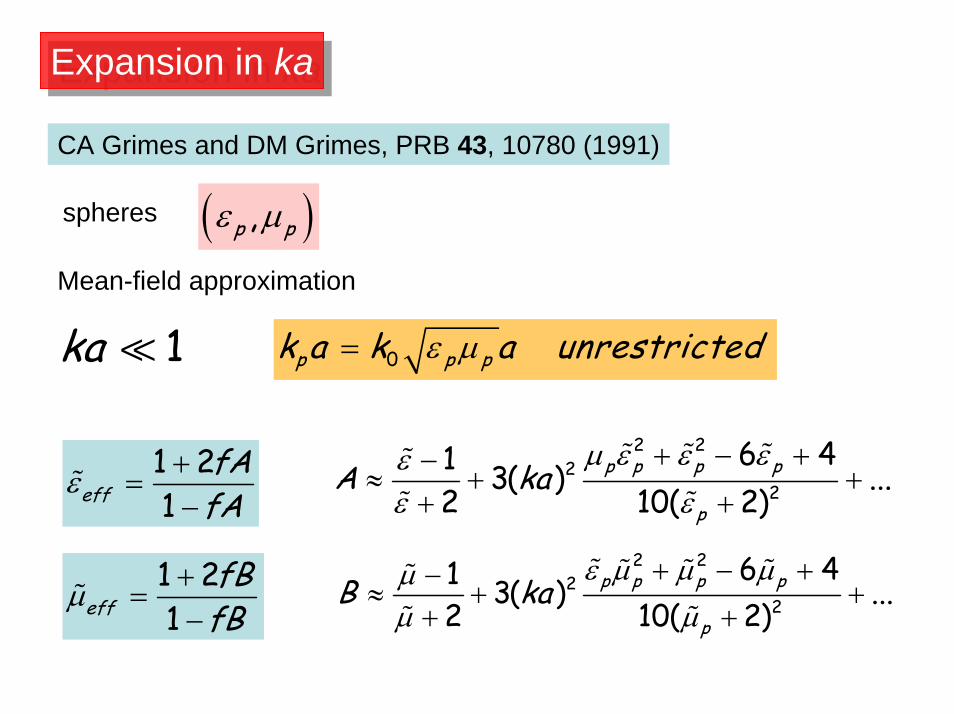
Expansion in kaExpansion in ka

CA Grimes and DM Grimes, PRB 43, 10780 (1991)

( ),p pε µspheres

Mean-field approximation

1ka 0p p pk a k a unrestrictedε µ=

2 22

2

6 41 3( ) ...2 10( 2)

p p p p

pA ka

µ ε ε εεε ε

+ − +−≈ + +

+ +1 21eff

fAfA

ε +=

−

2 22

2

6 41 3( ) ...2 10( 2)

p p p p

pB ka

ε µ µ µµµ µ

+ − +−≈ + +

+ +1 21eff

fBfB

µ +=

−

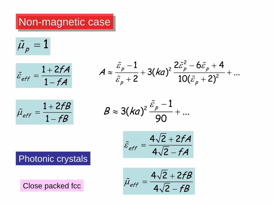
Non-magnetic caseNon-magnetic case

1pµ =2

22

1 2 6 43( ) ...

2 10( 2)p p p

p pA ka

ε ε εε ε

− − +≈ + +

+ +1 21eff

fAfA

ε +=

−

2 13( ) ...

90pB kaε −

≈ +1 21eff

fBfB

µ +=

−

4 2 24 2eff

fAfA

ε +=

−Photonic crystals

4 2 24 2eff

fBfB

µ +=

−Close packed fcc

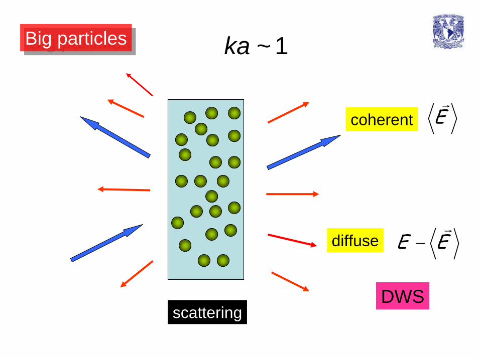
Big particlesBig particles ~ 1ka

Ecoherent

E E−diffuse

DWSscattering

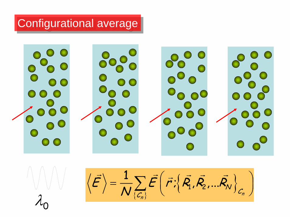
Configurational averageConfigurational average

1 21 ; , , ...

nn

N CCE E r R R R

N⎛ ⎞= ⎜ ⎟⎝ ⎠∑

0λ

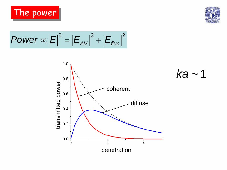
The powerThe power

∝ = +2 2 2

AV flucPower E E E

~ 1ka

0 2 40.0

0.2

0.4

0.6

0.8

1.0

diffuse

coherent

penetration

trans

mitt

ed p

ower

γ= +1 (0)eff

S

n i Sn

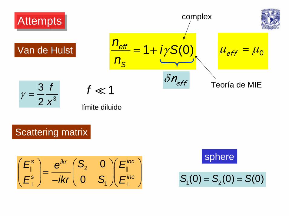
AttemptsAttempts

effnδ1f

complex

0effµ µ=Van de Hulst

Teoría de MIEγ = 3

32

fx límite diluido

Scattering matrix

⊥ ⊥

⎛ ⎞ ⎛ ⎞⎛ ⎞=⎜ ⎟ ⎜ ⎟⎜ ⎟− ⎝ ⎠⎝ ⎠ ⎝ ⎠

2

1

00

s incikr

s inc

SE EeSikrE E

sphere

= =1 2(0) (0) (0)S S S

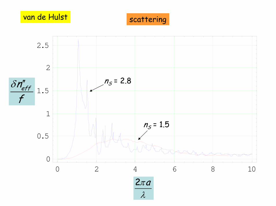
van de Hulst scattering

0 2 4 6 8 100

0.5

1

1.5

2

2.5

effnf

δ ′′

nS = 1.5

nS = 2.8

2 aπλ

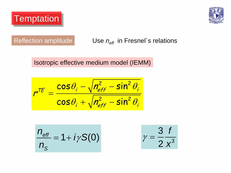
TemptationTemptation

Reflection amplitude Use neff in Fresnel´s relations

Isotropic effective medium model (IEMM)

2 2

2 2

cos sincos sin

i ieffTE

i ieff

nr

nθ θ

θ θ

− −=

+ −

γ = 3

32

fx

γ= +1 (0)eff

S

n i Sn

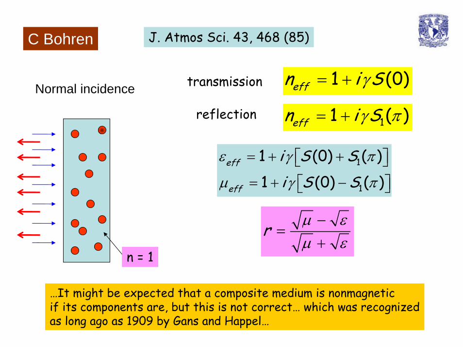
C Bohren J. Atmos Sci. 43, 468 (85)

1 (0)effn i Sγ= +transmissionNormal incidence

11 ( )effn i Sγ π= +reflection

1

1

1 (0) ( )1 (0) ( )

eff

eff

i S Si S S

ε γ π

µ γ π

= + +⎡ ⎤⎣ ⎦= + −⎡ ⎤⎣ ⎦

r µ εµ ε−

=+

n = 1

…It might be expected that a composite medium is nonmagneticif its components are, but this is not correct… which was recognizedas long ago as 1909 by Gans and Happel…

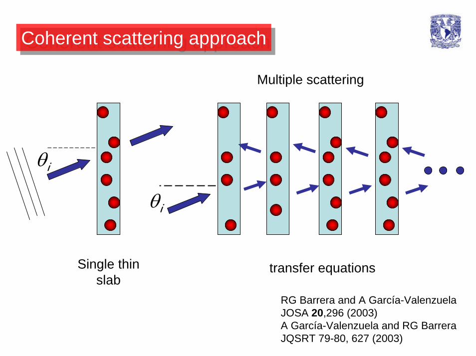
Coherent scattering approachCoherent scattering approach

Multiple scattering

iθ

iθ

Single thinslab

transfer equations

RG Barrera and A García-ValenzuelaJOSA 20,296 (2003)A García-Valenzuela and RG BarreraJQSRT 79-80, 627 (2003)

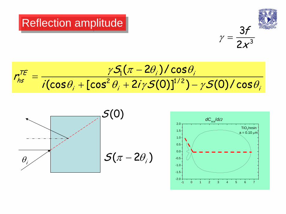
Reflection amplitudeReflection amplitude3

32

fx

γ =

12 1/2

( 2 )/cos(cos [cos 2 (0)] ) (0)/cos

TE i ihs

i i i

Sri i S S

γ π θ θθ θ γ γ θ

−=

+ + −

(0)S

( 2 )iS π θ−

-1 0 1 2 3 4 5 6 7-2.0

-1.5

-1.0

-0.5

0.0

0.5

1.0

1.5

2.0 TiO2/resina = 0.10 µm

dCsca/dΩ

iθ

ValidationValidation

Theory

Extension toinclude the matrix

Experiment

Internal reflectionConfiguration

great sensitivityA García-Valenzuela, RG Barrera,C. Sánchez-Pérez, A. Reyes-Coronado,E Méndez, Optics Express, 13, 6723 (2005)

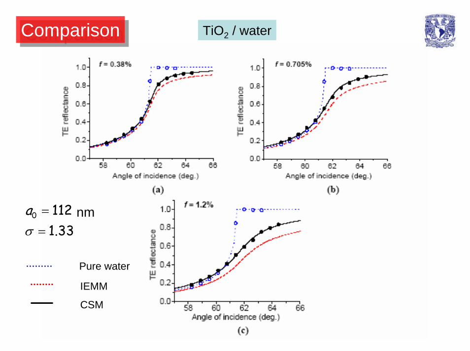
ComparisonComparison TiO2 / water

Pure water

IEMM

CSM

0 1121.33

aσ

=

=nm

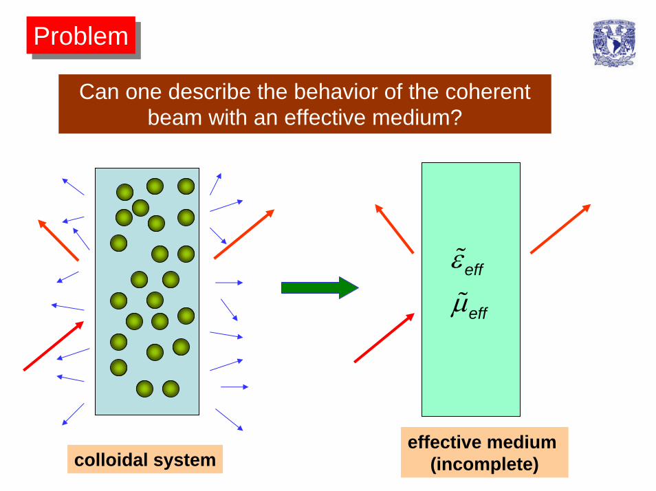
ProblemProblem

Can one describe the behavior of the coherentbeam with an effective medium?

effective medium (incomplete)colloidal system

eff

eff

εµ

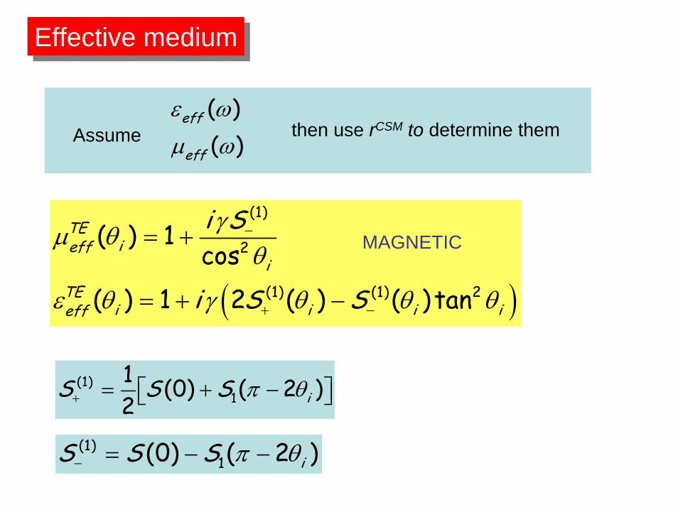
Effective mediumEffective medium

Assume( )( )

eff

eff

ε ωµ ω

then use rCSM to determine them

( )

(1)

2

(1) (1) 2

( ) 1cos

( ) 1 2 ( ) ( )tan

TEieff

iTE

i i i ieff

i S

i S S

γµ θθ

ε θ γ θ θ θ

−

+ −

= +

= + −

MAGNETIC

(1)1

1 (0) ( 2 )2 iS S S π θ+ = + −⎡ ⎤⎣ ⎦

(1)1(0) ( 2 )iS S S π θ− = − −

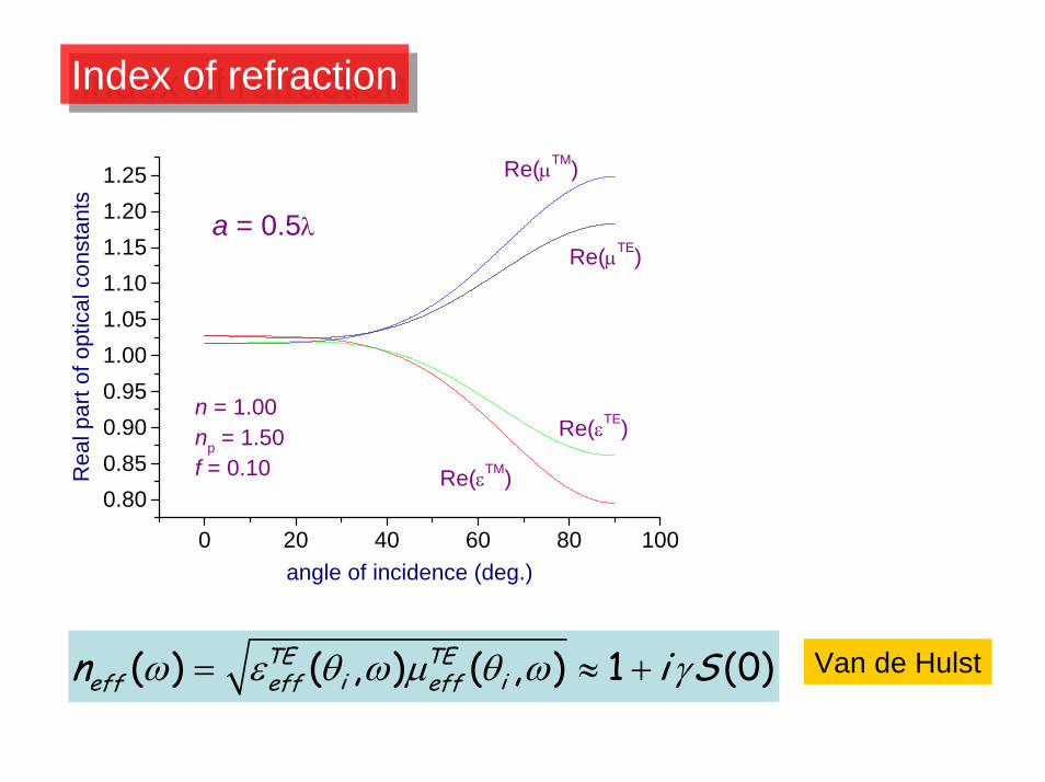
Index of refractionIndex of refraction

0 20 40 60 80 100

0.800.850.900.951.001.051.101.151.201.25

a = 0.5λ

n = 1.00np = 1.50f = 0.10 Re(εTM)

Re(µTM)

Re(εTE)

Re(µTE)

Rea

l par

t of o

ptic

al c

onst

ants

angle of incidence (deg.)

( ) ( , ) ( , ) 1 (0)TE TEi ieff eff effn i Sω ε θ ω µ θ ω γ= ≈ + Van de Hulst

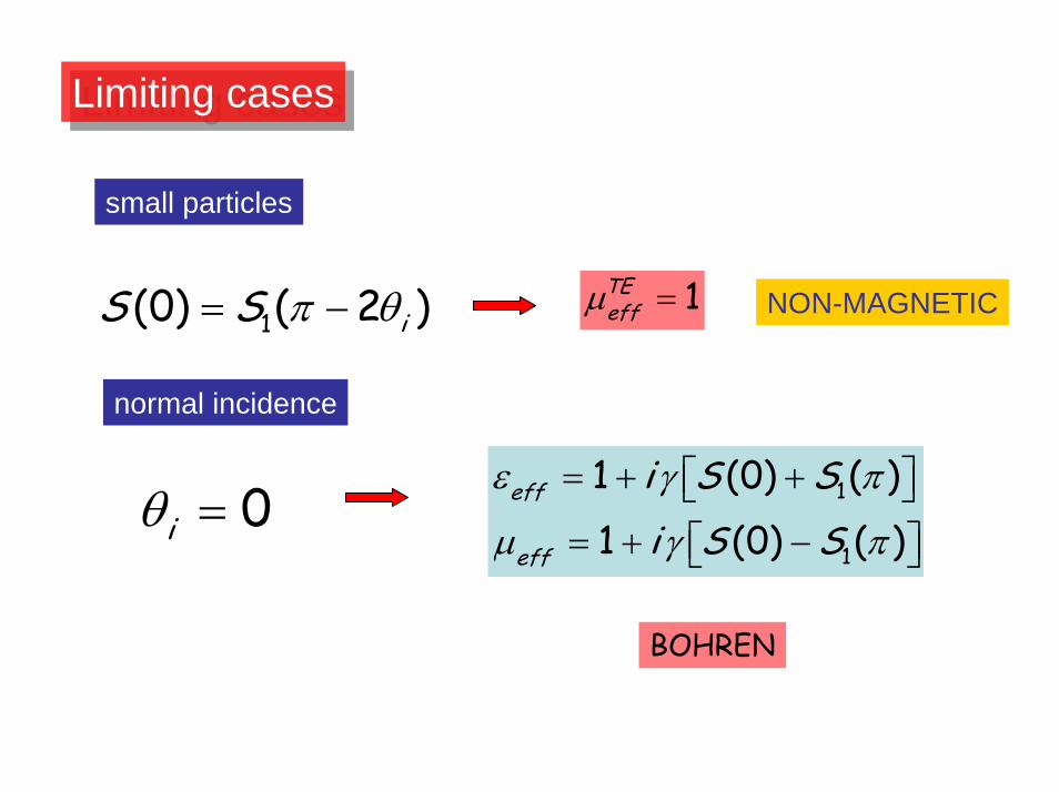
Limiting casesLimiting cases

small particles

1TEeffµ =

1(0) ( 2 )iS S π θ= − NON-MAGNETIC

normal incidence

1

1

1 (0) ( )1 (0) ( )

eff

eff

i S Si S S

ε γ π

µ γ π

= + +⎡ ⎤⎣ ⎦= + −⎡ ⎤⎣ ⎦

0iθ =

BOHREN

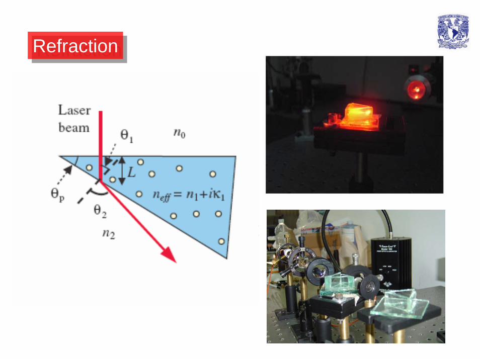
RefractionRefraction

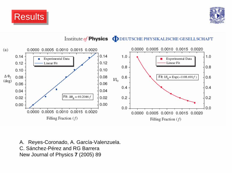
ResultsResults

A. Reyes-Coronado, A. García-Valenzuela.C. Sánchez-Pérez and RG BarreraNew Journal of Physics 7 (2005) 89

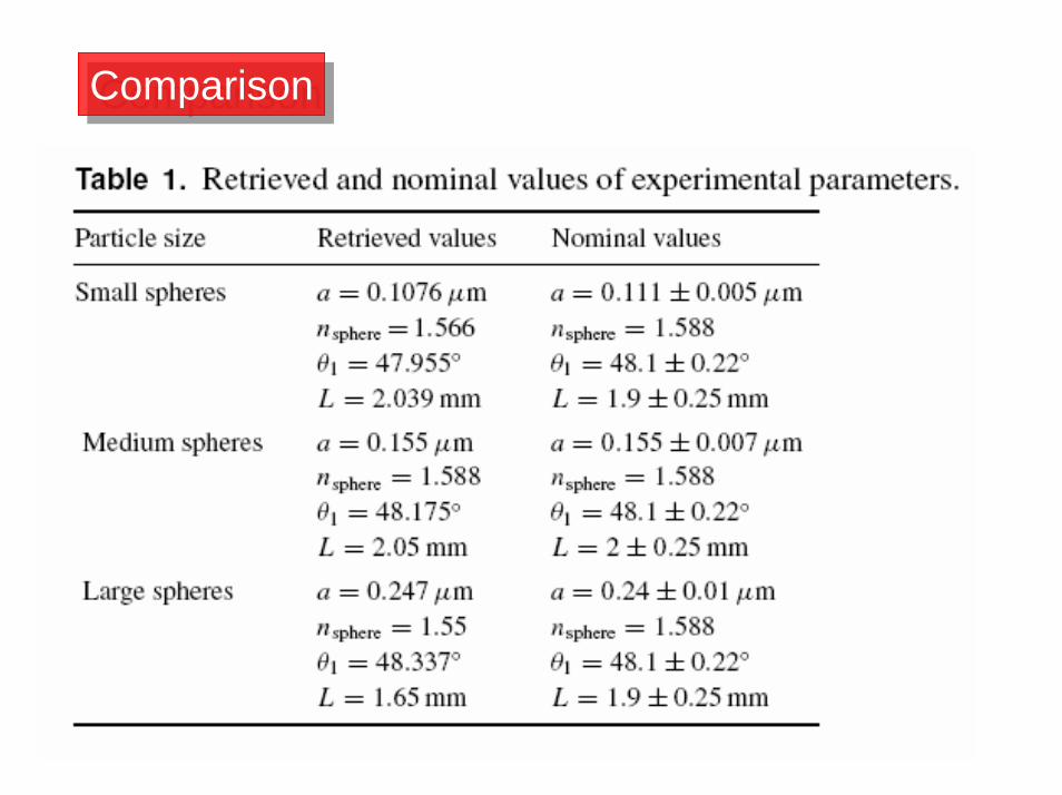
ComparisonComparison

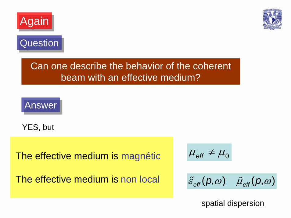
AgainAgain

QuestionQuestion

Can one describe the behavior of the coherentbeam with an effective medium?

AnswerAnswer

YES, but

The effective medium is magnétic

The effective medium is non local

µ µ≠ 0eff

( , ) ( , )eff effp pε ω µ ω

spatial dispersion

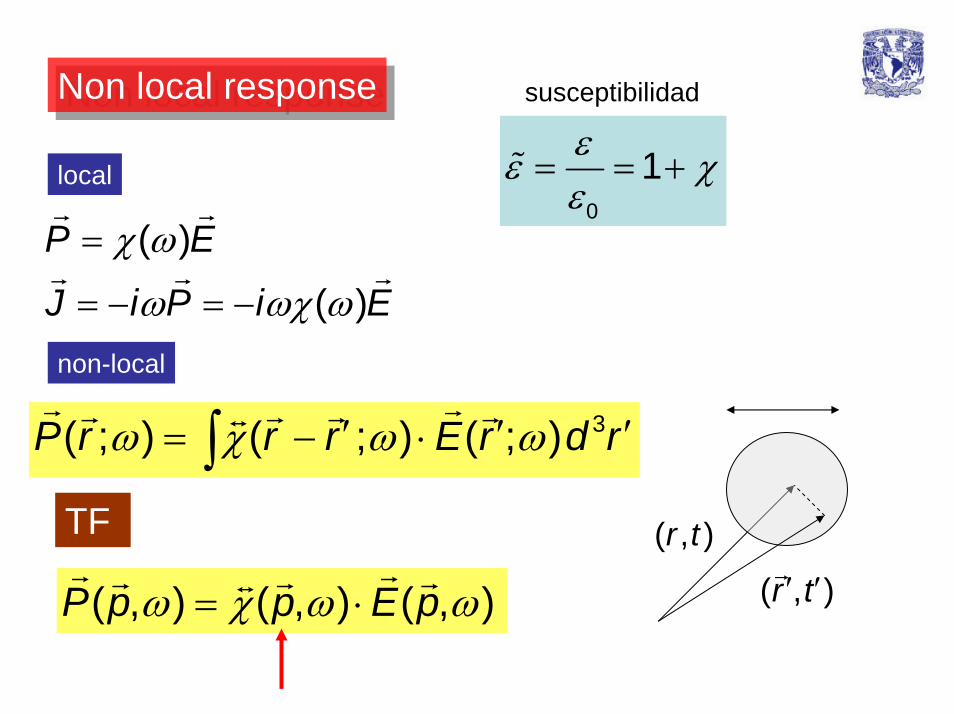
Non local responseNon local response

0

1εε χε

= = +

χ ω

ω ωχ ω

=

= − = −

( )

( )

P E

J i P i E

3( ; ) ( ; ) ( ; )P r r r E r d rω χ ω ω′ ′ ′= − ⋅∫TF

ω χ ω ω= ⋅( , ) ( , ) ( , )P p p E p

( , )r t

( , )r t′ ′

susceptibilidad

local

non-local

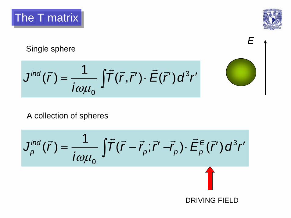
The T matrixThe T matrix

ESingle sphere

3

0

1( ) ( , ) ( )indJ r T r r E r d riωµ

′ ′ ′= ⋅∫

A collection of spheres

ωµ′ ′ ′= − − ⋅∫ 3

0

1( ) ( ; ) ( )ind Ep p p pJ r T r r r r E r d r

i

DRIVING FIELD

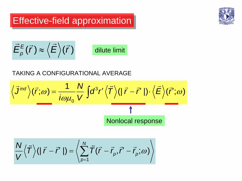
Effective-field approximationEffective-field approximation

( ) ( )EpE r E r≈ dilute limit

TAKING A CONFIGURATIONAL AVERAGE

3

0

1( ; ) (| |) ( ; )ind NJ r d r T r r E ri V

ω ωωµ

′ ′ ′= − ⋅∫

Nonlocal response

1(| |) ( , ; )

N

p pp

N T r r T r r r rV

ω=

′ ′− = − −∑

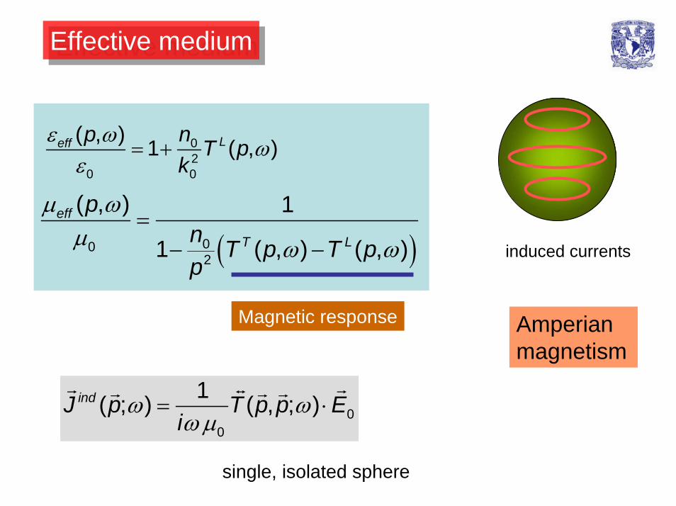
Effective mediumEffective medium

ε ωω

ε= + 0

20 0

( , ) 1 ( , )Leff p n T pk

( )µ ω

µ ω ω=

− −002

( , ) 1

1 ( , ) ( , )

eff

T L

pn T p T pp

induced currents

Magnetic response Amperianmagnetism

00

1( ; ) ( , ; )indJ p T p p Ei

ω ωω µ

= ⋅

single, isolated sphere

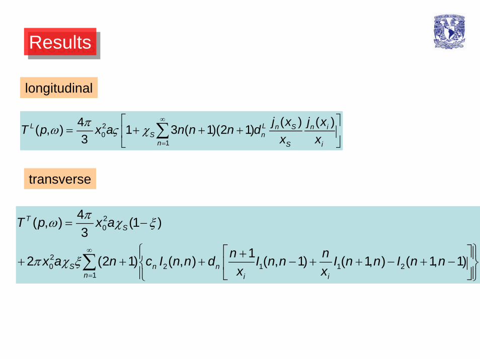
ResultsResults

longitudinal

20

1

( ) ( )4( , ) 1 3 ( 1)(2 1)3

L L n S n iS n

n S i

j x j xT p x a n n n dx x

πω ς χ∞

=

⎡ ⎤= + + +⎢ ⎥

⎣ ⎦∑

transverse

20

20 2 1 1 2

1

4( , ) (1 )3

12 (2 1) ( , ) ( , 1) ( 1, ) ( 1, 1)

TS

S n nn i i

T p x a

n nx a n c I n n d I n n I n n I n nx x

πω χ ξ

π χ ξ∞

=

= −

⎧ ⎫⎡ ⎤+⎪ ⎪+ + + − + + − + −⎨ ⎬⎢ ⎥⎪ ⎪⎣ ⎦⎩ ⎭

∑

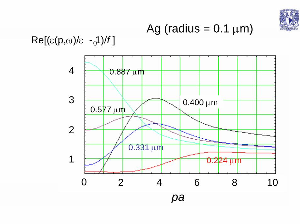
Ag (radius = 0.1 µm)

2 4 6 8 100

1

2

3

4

Re[(ε(p,ω)/ε - 1)/f ] 0

pa

0.224 µm0.331 µm

0.400 µm 0.577 µm

0.887 µm

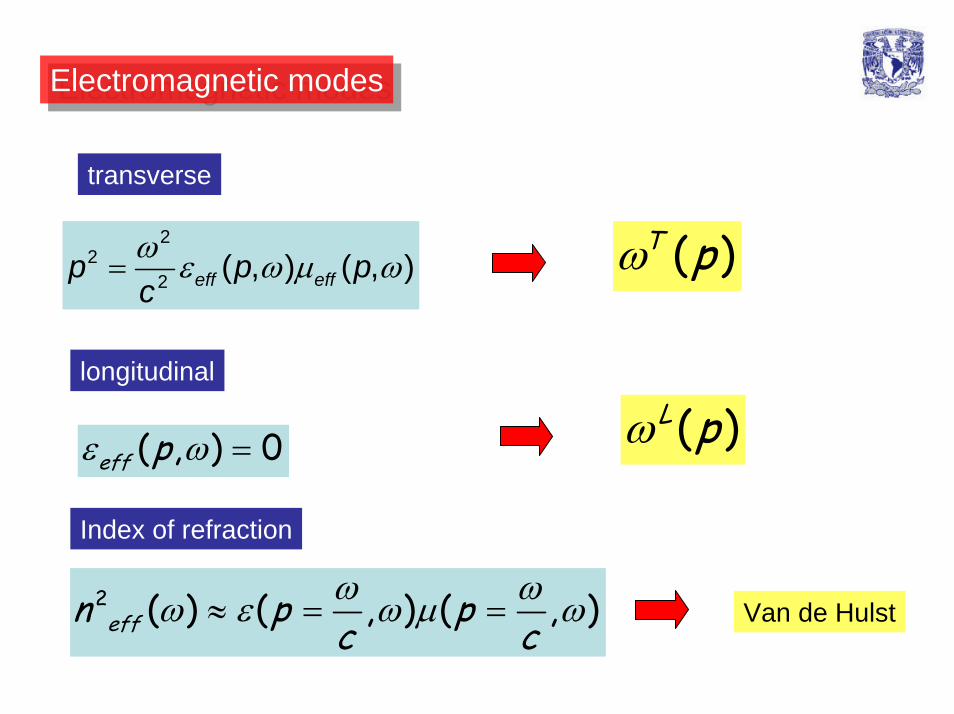
Electromagnetic modesElectromagnetic modes

transverse

( )T pωω ε ω µ ω=2

22 ( , ) ( , )eff effp p p

c

longitudinal

( )L pω( , ) 0eff pε ω =

Index of refraction

2 ( ) ( , ) ( , )effn p pc cω ωω ε ω µ ω≈ = = Van de Hulst

λ [µm]0

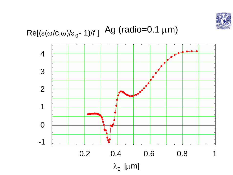
Re[(ε(ω/c,ω)/ε - 1)/f ] 0Ag (radio=0.1 µm)

0.2 0.4 0.6 0.8 1

0

1

2

3

4

-1

0.2 0.4 0.6 0.8 1

l0 @mm D

0.99

1

1.01

1.02

Re mH p=k0,wL

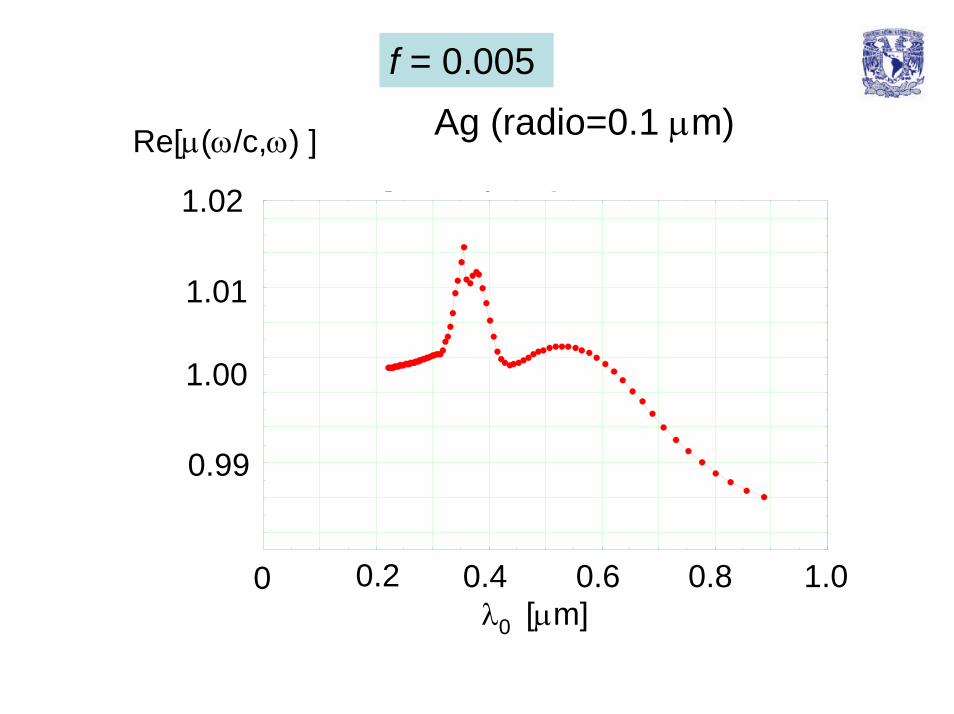
mH p=k0,wL for Ag with radius =0.1Ag (radio=0.1 µm)

λ [µm]0

0.2 0.4 0.6 0.8 1.00

0.99

1.00

1.01

1.02

Re[µ(ω/c,ω) ]

f = 0.005

Actual researchActual research

We are working on the non local properties of theelectromagnetic response of colloidal systems andWe are also performing refraction and reflectionexperiments in order to design an instrument to measurethe particle-size distribution of colloidal particles usingthe information stored in the coherent beam.

We are building up a group on optical propertiers at anindustrial lab of the paint industry, where we are applyingsome of the results obtained in our basic-researchstudies.