optical metrology - andres marrugo

Optical MetrologyLecture 2: Random Data and Characterization of

Measurement Systems

Content of the Lecture

• Deterministic Data.

• Random Data.

• Characteristics of Random Data.

• Characterization of measurement systems.

• Static and Dynamic characterization.

Deterministic versus Random Data

2 BASIC DESCRIPTIONS AND PROPERTIES

Position of equilibrium

m

x(0

Figure 1.1 Simple spring mass system.

There are many physical phenomena in practice that produce data that can be represented with reasonable accuracy by explicit mathematical relationships. For example, the motion of a satellite in orbit about the earth, the potential across a condenser as it discharges through a resistor, the vibration response of an unbalanced rotating machine, and the temperature of water as heat is applied are all basically deterministic. However, there are many other physical phenomena that produce data that are not deterministic. For example, the height of waves in a confused sea, the acoustic pressures generated by air rushing through a pipe, and the electrical output of a noise generator represent data that cannot be described by explicit mathematical relationships. There is no way to predict an exact value at a future instant of time. These data are random in character and must be described in terms of probability statements and statistical averages rather than by explicit equations.

The classification of various physical data as being either deterministic or random might be debated in many cases. For example, it might be argued that no physical data in practice can be truly deterministic because there is always a possibility that some unforeseen event in the future might influence the phenomenon producing the data in a manner that was not originally considered. On the other hand, it might be argued that no physical data are truly random, because an exact mathematical description might be possible if a sufficient knowledge of the basic mechanisms of the phenomenon producing the data were available. In practical terms, the decision of whether physical data are deterministic or random is usually based on the ability to reproduce the data by controlled experiments. If an experiment producing specific data of interest can be repeated many times with identical results (within the limits of experimental error), then the data can generally be considered deterministic. If an experiment cannot be designed that will produce identical results when the experiment is repeated, then the data must usually be considered random in nature.

Various special classifications of deterministic and random data will now be discussed. Note that the classifications are selected from an analysis viewpoint and do not necessarily represent the most suitable classifications from other possible view-points. Further note that physical data are usually thought of as being functions of time and will be discussed in such terms for convenience. Any other variable, however, can replace time, as required.

Deterministic Data• Any observed data

representing a physical phenomenon can be broadly classified as being either deterministic or nondeterministic.

• Deterministic data are those that can be described by an explicit mathematical relationship.

x(t) = X cos

rk

m

t t � 0

Classification of Deterministic Data

(Periódicoarbitrario)


Amplitude

X X I *-Time 0 Frequency

Figure 1.3 Time history and spectrum of sinusoidal data.

The frequency and period are related by

Note that the frequency spectrum in Figure 1.3 is composed of an amplitude component at a specific frequency, as opposed to a continuous plot of amplitude versus frequency. Such spectra are called discrete spectra or line spectra.

There are many examples of physical phenomena that produce approximately sinusoidal data in practice. The voltage output of an electrical alternator is one example; the vibratory motion of an unbalanced rotating weight is another. Sinusoidal data represent one of the simplest forms of time-varying data from the analysis viewpoint.

1.2.2 Complex Periodic Data

Complex periodic data are those types of periodic data that can be defined math-ematically by a time-varying function whose waveform exactly repeats itself at regular intervals such that

As for sinusoidal data, the time interval required for one full fluctuation is called the period Tp. The number of cycles per unit time is called the fundamentalfrequency j \ . A special case for complex periodic data is clearly sinusoidal data, where f\ =/0.

With few exceptions in practice, complex periodic data may be expanded into a Fourier series according to the following formula:

x{t) — x(t � nTp) � = 1 , 2 , 3 , . . . (1.5)

oo x(t) — + ^ ^ ( � � cos 2nnf\t + bn sin2%nf\t)

2 n=l (1.6)

where

0 , 1 , 2 , . . .

1 , 2 , 3 , . . .

Sinusoidalx(t) = X sin(2⇡f0t+ �)

Discrete spectra

f0 =1

Tp

CLASSIFICATIONS OF DETERMINISTIC DATA 5

An alternative way to express the Fourier series for complex periodic data is

oo

x{t) =� 0+� � � cos{2nnfi �-� � ) (1.7)

n = l

where

X 0 = a0/2

Xn = y/aJ+bJ n = l , 2 , 3 , . . .

0„ = t a n - 1 (£>„/««) n = l , 2 , 3 , . . . In words, Equation (1.7) says that complex periodic data consist of a static component Xq and an infinite number of sinusoidal components called harmonics, which have amplitudes XN and phases � � . The frequencies of the harmonic components are all integral multiples o f / j .

When analyzing periodic data in practice, the phase angles � � are often ignored. For this case, Equation (1.7) can be characterized by a discrete spectrum, as illustrated in Figure 1.4. Sometimes, complex periodic data will include only a few components. In other cases, the fundamental component may be absent. For example, suppose a periodic time history is formed by mixing three sine waves that have frequencies of 60, 75, and 100 Hz. The highest common divisor is 5 Hz, so the period of the resulting periodic data is TP = 0.2 s. Hence, when expanded into a Fourier series, all values of XN

are zero except for � = 12, � = 15, and � = 20. Physical phenomena that produce complex periodic data are far more common

than those that produce simple sinusoidal data. In fact, the classification of data as being sinusoidal is often only an approximation for data that are actually complex. For example, the voltage output from an electrical alternator may actually display, under careful inspection, some small contributions at higher harmonic frequencies. In other cases, intense harmonic components may be present in periodic physical data. For example, the vibration response of a multicyclinder reciprocating engine will usually display considerable harmonic content.

Amplitude

•X2

� Xs

h 2fi 3 A 4/"� 5�

Figure 1.4 Spectrum of complex periodic data.

• Frequency

Complex Periodic(Arbitrario)

x(t) = X(t± nTp), n = 1, 2, 3, . . .

f1 =1

Tp

Data consists of a static component X0 and an infinite number of sinusoidal components called harmonics. integral multiples of f1.

Almost-periodic


1.2.3 Almost-Periodic Data

In Section 1.2.2, it is noted that periodic data can generally be reduced to a series of sine waves with commensurately related frequencies. Conversely, the data formed by summing two or more commensurately related sine waves will be periodic. However, the data formed by summing two or more sine waves with arbitrary frequencies generally will not be periodic. Specifically, the sum of two or more sine waves will be periodic only when the ratios of all possible pairs of frequencies form rational numbers. This indicates that a fundamental period exists that will satisfy the requirements of Equation (1.5). Hence,

x(t) = Xi sin(2r + 0 i ) + X 2 s i n ( 3 / + 0 2 ) + X 3 s i n ( 7 i + 03)

is periodic because | , � , and � are rational numbers (the fundamental period is Tp=\). On the other hand,

x(t) =Xi sin(2r + 0 1 ) + X 2 S i n ( 3 r + 0 2 ) + X 3 s i n ( v / 5 O r + 0 3 )

is not periodic because 2/\/50 and 3 / v/50 are not rational numbers (the fundamental period is infinitely long). The resulting time history in this case will have an almost-periodic character, but the requirements of Equation (1.5) will not be satisfied for any finite value of Tp.

Based on these discussions, almost-periodic data are those types of nonperiodic data that can be defined mathematically by a time-varying function of the form

� (� =� � � � � (2� /� � + � � ) (1.8) n = 1

where fn/fm � rational number in all cases. Physical phenomena producing almost-periodic data frequently occur in practice when the effects of two or more unrelated periodic phenomena are mixed. A good example is the vibration response in a multiple-engine propeller airplane when the engines are out of synchronization.

An important property of almost-periodic data is as follows. If the phase angles 0„ are ignored, Equation (1.8) can be characterized by a discrete frequency spectrum similar to that for complex periodic data. The only difference is that the frequencies of the components are not related by rational numbers, as illustrated in Figure 1.5.

Amplitude

rXi

frequency

Figure 1.5 Spectrum of almost-periodic data.

No relation

Transient Nonperiodic DataCLASSIFICATIONS OF DETERMINISTIC DATA 7

Figure 1.6 Illustrations of transient data.

1.2.4 Transient Nonperiodic Data

Transient data are defined as all nonperiodic data other than the almost-periodic data discussed in Section 1.2.3. In other words, transient data include all data not previously discussed that can be described by some suitable time-varying function. Three simple examples of transient data are given in Figure 1.6.

Physical phenomena that produce transient data are numerous and diverse. For example, the data in Figure 1.6(a) could represent the temperature of water in a kettle (relative to room temperature) after the flame is turned off. The data in Figure 1.6(b) might represent the free vibration of a damped mechanical system after an excitation force is removed. The data in Figure 1.6(c) could represent the stress in an end-loaded cable that breaks at time c.

An important characteristic of transient data, as opposed to periodic and almost-periodic data, is that a discrete spectral representation is not possible A continuous spectral representation for transient data can be obtained in most cases, however, from a Fourier transform given by

x(f) = x(t)e-J27lftdt (1.9)

The Fourier transform X(f) is generally a complex number that can be expressed in complex polar notation as

� �/) = \m\e -J6if)

Here, \X(f)\ is the magnitude of X(f) and #(/) is the argument. In terms of the magnitude \X(f)\, continuous spectra of the three transient time histories in Figure 1.6 are as presented in Figure 1.7. Modern procedures for the digital computation of Fourier series and finite Fourier transforms are detailed in Chapter 11.


f

Figure 1.7 Spectra of transient data.

1.3 CLASSIFICATIONS OF RANDOM DATA

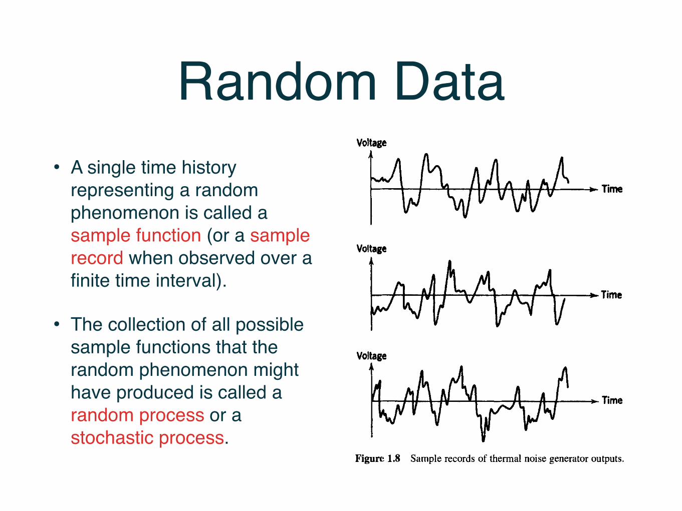
As discussed earlier, data representing a random physical phenomenon cannot be described by an explicit mathematical relationship because each observation of the phenomenon will be unique. In other words, any given observation will represent only one of many possible results that might have occurred. For example, assume the output voltage from a thermal noise generator is recorded as a function of time. A specific voltage time history record will be obtained, as shown in Figure 1.8. If a second thermal noise generator of identical construction and assembly is operated simultaneously, however, a different voltage time history record would result. In fact, every thermal noise generator that might be constructed would produce a different voltage time history record, as illustrated in Figure 1.8. Hence, the voltage time history for any one generator is merely one example of an infinitely large number of time histories that might have occurred.

A single time history representing a random phenomenon is called a sample function (or a sample record when observed over a finite time interval). The collection of all possible sample functions that the random phenomenon might have produced is called a random process or a stochastic process. Hence, a sample record of data for a random physical phenomenon may be thought of as one physical realization of a random process.

Random processes may be categorized as being either stationary or nonstationary. Stationary random processes may be further categorized as being either ergodic or nonergodic. Nonstationary random processes may be further categorized in terms of

Continuous spectral representation.

How do you approximate sampling?

Classification of Random Data

CLASSIFICATIONS OF RANDOM DATA 9

Voltage

Time

Voltage

-•-Time

Time

Figure 1.8 Sample records of thermal noise generator outputs.

specific types of nonstationary properties. These various classifications of random processes are schematically illustrated in Figure 1.9. The meaning and physical significance of these various types of random processes will now be discussed in broad terms. More analytical definitions and developments are presented in Chapters 5 and 12.

1.3.1 Stationary Random Data

When a physical phenomenon is considered in terms of a random process, the properties of the phenomenon can hypothetically be described at any instant of time by computing

Stationary

I Nonstationary

Ergodic Nonergodtc Special

classifications of nonstationarrty

Figure 1.9 Classifications of random data.

Random Data• A single time history

representing a random phenomenon is called a sample function (or a sample record when observed over a finite time interval).

• The collection of all possible sample functions that the random phenomenon might have produced is called a random process or a stochastic process.


*t<t)

* 2 W

' I * / 1

I—� � —. Figure 1.10 Ensemble of time history records defining a random process.

average values over the collection of sample functions that describe the random process. For example, consider the collection of sample functions (also called the ensemble) that forms the random process illustrated in Figure 1.10. The mean value (first moment) of the random process at some ti can be computed by taking the instantaneous value of each sample function of the ensemble at time ri, summing the values, and dividing by the number of sample functions. In a similar manner, a correlation (joint moment) between the values of the random process at two different times (called the autocorrelation function) can be computed by taking the ensemble average of the product of instant-aneous values at two times, t\ andi] -I- � . That is, for the random process {*(?)}, where thesymbol {} is used to denote an ensemble of sample functions, the mean value ^ f ^ a n d the autocorrelation function R^ (tx, t\ + � ) are given by

1 N

� � {*�) = A , l i m I? � k� 1

(1.10a)

1 N

Rxx(h,h +� ) = lim - YV(fi)**(ii + T ) (1.10b) � � > oo i v f—,

k=\ where the final summation assumes that each sample function is equally likely.


*t<t)

* 2 W

' I * / 1



1 N

� � {*�) = A , l i m I? � k� 1

(1.10a)

1 N



• A random process can be described by computing average values over the collection of sample functions

• If and vary with t1, the process is non-stationary.


*t<t)

* 2 W

' I * / 1



1 N

� � {*�) = A , l i m I? � k� 1

(1.10a)

1 N



Stationary Random Data


*t<t)

* 2 W

' I * / 1



1 N

� � {*�) = A , l i m I? � k� 1

(1.10a)

1 N



Ergodic Random Data

• A sample can be taken out of any signal, or across a signal and it will be representative of the event.

• This example could be turbulence across 4 flights in similar conditions with similar aircraft.

Analysis of Random Data• Basic statistical properties of importance for describing single

stationary random records are:

• Mean, mean square values, and moments of order n

• Probability density functions

• Autocorrelation functions

• Autospectral density functions

• Joint probability density functions

• Cross-correlation functions

ANALYSIS OF RANDOM DATA 15

(d)

Figure 1.11 Four special time histories, (a) Sine wave, (b) Sine wave plus random noise, (c) Narrow bandwidth random noise, (d) Wide bandwidth random noise.

The first three functions measure fundamental properties shared by the pair of records in the amplitude, time, or frequency domains. From knowledge of the cross-spectral density function between the pair of records, as well as their individual autospectral density functions, one can compute theoretical linear frequency response functions (gain factors and phase factors) between the two records. Here, the two records are treated as a single-input/single-output problem. The coherence function is a measure of the accuracy of the assumed linear input/output model and can also be computed from the measured autospectral and cross-spectral density functions. Detailed discussions of these topics appear in Chapters 5, 6, and 7.


Figure 1.12 Probability density function plots, (a) Sine wave, (b) Sine wave plus random noise, (c) Narrow bandwidth random noise, (d) Wide bandwidth random noise.

Common applications of probability density and distribution functions, beyond a basic probabilistic description of data values, include

1. Evaluation of normality

2. Detection of data acquisition errors

3. Indication of nonlinear effects

4. Analysis of extreme values

Probability density functions


(d)



Autocorrelation functions

Figure 1.13 Autocorrelation function plots, (a) Sine wave, (b) Sine wave plus random noise, (c) Narrow bandwidth random noise, (d) Wide bandwidth random noise.


(d)



Autospectral density functions18 BASIC DESCRIPTIONS AND PROPERTIES

Figure 1.14 Autospectral density function plots, (a) Sine wave, (b) Sine wave plus random noise, (c) Narrow bandwidth random noise, (d) Wide bandwidth random noise.

The primary applications of correlation measurements include

1. Detection of periodicities

2. Prediction of signals in noise

3. Measurement of time delays

4. Location of disturbing sources

5. Identification of propagation paths and velocities

Characterization of Measurement Systems

A simple instrument model

• An observable variable X is obtained from the measurand.

• X is related to the measurand in some KNOWN way (i.e., measuring mass)

• The sensor generates a signal variable that can be manipulated:

• Processed, transmitted or displayed

• In the example above the signal is passed to a display, where a measurement can be taken

Intelligent Sensor SystemsRicardo Gutierrez-OsunaWright State University

3

MeasurementsA simple instrument model

A observable variable X is obtained from the measurandX is related to the measurand in some KNOWN way (i.e., measuring mass)

The sensor generates a signal variable that can be manipulated:Processed, transmitted or displayed

In the example above the signal is passed to a display, where a measurement can be taken

MeasurementThe process of comparing an unknown quantity with a standard of the same quantity (measuring length) or standards of two or more related quantities (measuring velocity)

Sensor

Physical measurement

variable

X

Signalvariable

S

Measurement

MMeasurand

PHYSICALPROCESS

DisplaySensor


variable

X

Signalvariable

S

Measurement

MMeasurand

PHYSICALPROCESS

Measurand

PHYSICALPROCESS

Display


A simple instrument model

Measurement

• The process of comparing an unknown quantity with a standard of the same quantity (measuring length) or standards of two or more related quantities (measuring velocity)


3

MeasurementsA simple instrument model

A observable variable X is obtained from the measurandX is related to the measurand in some KNOWN way (i.e., measuring mass)

The sensor generates a signal variable that can be manipulated:Processed, transmitted or displayed

In the example above the signal is passed to a display, where a measurement can be taken

MeasurementThe process of comparing an unknown quantity with a standard of the same quantity (measuring length) or standards of two or more related quantities (measuring velocity)

Sensor


variable

X

Signalvariable

S

Measurement

MMeasurand

PHYSICALPROCESS

DisplaySensor


variable

X

Signalvariable

S

Measurement

MMeasurand

PHYSICALPROCESS

Measurand

PHYSICALPROCESS

Display


4

CalibrationThe relationship between the physical measurement variable (X) and the signal variable (S)

A sensor or instrument is calibrated by applying a number of KNOWN physical inputs and recording the response of the system

Physical input (X)

Sign

al o

utpu

t (Y)

Physical input (X)

Sign

al o

utpu

t (Y)


The relationship between the physical measurement variable (X) and the signal variable (S)

• A sensor or instrument is calibrated by applying a number of KNOWN physical inputs and recording the response of the system.


5

Additional inputsInterfering inputs (Y)

Those that the sensor to respond as the linear superposition with the measurand variable X

Linear superposition assumption: S(aX+bY)=aS(X)+bS(Y)

Modifying inputs (Z)Those that change the behavior of the sensor and, hence, the calibration curve

Temperature is a typical modifying input

Sign

al o

utpu

t (Y)

Physical input (X)

Z=Z1

Z=Z2

Sensor

Physical variable X Signalvariable

SMeasurand Interfering input Y

Modifying input Z

Sensor


SMeasurandMeasurand Interfering input Y

Modifying input Z


Interfering inputs (Y)

• Those that the sensor to respond as the linear superposition with the measurand variable X.

• Linear superposition assumption: S(aX+bY)=aS(X)+bS(Y)


Modifying inputs (Z)

• Those that change the behavior of the sensor and, hence, the calibration curve

• Temperature is a typical modifying input.


5

Additional inputsInterfering inputs (Y)

Those that the sensor to respond as the linear superposition with the measurand variable X

Linear superposition assumption: S(aX+bY)=aS(X)+bS(Y)

Modifying inputs (Z)Those that change the behavior of the sensor and, hence, the calibration curve

Temperature is a typical modifying inputSi

gnal

out

put (

Y)

Physical input (X)

Z=Z1

Z=Z2

Sensor


SMeasurand Interfering input Y

Modifying input Z

Sensor


SMeasurandMeasurand Interfering input Y

Modifying input Z


Static characteristics

•The properties of the system after all transient effects have settled to their final or steady state.

•Accuracy

•Discrimination

•Precision

•Errors

•Drift

•Sensitivity

•Linearity

•Hystheresis

Dynamic characteristics

• The properties of the system transient response to an input.

• Zero order systems.

• First order systems.

• Second order systems.


Ejemplo - Calibración

• Ejemplo. Un sistema de medida de altura usando pulsos de luz. La tabla muestra los valores reales y los medidos (con error) cuando se incrementa la distancia y cuando se disminuye.

Ejemplo - Calibración

• In general when f is a function of x,y,z,

Combination of errors

3.2 ERROR PROPAGATION 21

Table 3.1 Propagation of standard uncertainties in combinedquantities or functions.

f = x + y or f = x − y σ 2f = σ 2

x + σ 2y

f = xy or f = x/y (σf /f )2 = (σx/x)2 + (σy/y)2

f = xyn or f = x/yn (σf /f )2 = (σx/x)2 + n2(σy/y)2

f = ln x σf = σx/xf = ex σf = fσx

sources can be either + or − and will often partly compensate each other.The correct way to “add up” uncertainties is to take the square root of thesum of the squares of the individual uncertainties. More specifically, thisapplies to standard deviations σ :

If f = x + y, then σ 2f = σ 2

x + σ 2y , (3.4)

i.e., independent uncertainties add up quadratically. Why this is so isexplained in Appendix A1 on page 135. In general, when f is a functionof x, y, z, . . .;

σ 2f =

(∂f∂x

)2

σ 2x +

(∂f∂y

)2

σ 2y + · · · (3.5)

From (3.5) it follows immediately that for additions and subtractions theabsolute uncertainties add up quadratically, while for multiplications anddivisions the relative uncertainties add up quadratically. Examples of (3.5)are given in Table 3.1, valid for independent contributions.

Example 1

Consider the example of (3.2). What is the s.d. in K = [A2]/[A]2 when thedeviations in [A] and [A2] are independent? From the x/yn rule in Table 3.1it follows that

(σK

K

)2=

(σ[A2][A2]

)2

+ 4(

σ[A][A]

)2

.

Suppose you have measured [A2] = 0.010 ± 0.001 mol/L and [A] = 0.100 ±0.004 mol/L. Then the relative s.d. of K becomes

√0.12 + 4.0.042 = 0.13,

resulting in K = 1.0 ± 0.1 L/mol.

3.2 ERROR PROPAGATION 21

Table 3.1 Propagation of standard uncertainties in combinedquantities or functions.

f = x + y or f = x − y σ 2f = σ 2

x + σ 2y

f = xy or f = x/y (σf /f )2 = (σx/x)2 + (σy/y)2

f = xyn or f = x/yn (σf /f )2 = (σx/x)2 + n2(σy/y)2

f = ln x σf = σx/xf = ex σf = fσx

sources can be either + or − and will often partly compensate each other.The correct way to “add up” uncertainties is to take the square root of thesum of the squares of the individual uncertainties. More specifically, thisapplies to standard deviations σ :

If f = x + y, then σ 2f = σ 2

x + σ 2y , (3.4)

i.e., independent uncertainties add up quadratically. Why this is so isexplained in Appendix A1 on page 135. In general, when f is a functionof x, y, z, . . .;

σ 2f =

(∂f∂x

)2

σ 2x +

(∂f∂y

)2

σ 2y + · · · (3.5)

From (3.5) it follows immediately that for additions and subtractions theabsolute uncertainties add up quadratically, while for multiplications anddivisions the relative uncertainties add up quadratically. Examples of (3.5)are given in Table 3.1, valid for independent contributions.

Example 1

Consider the example of (3.2). What is the s.d. in K = [A2]/[A]2 when thedeviations in [A] and [A2] are independent? From the x/yn rule in Table 3.1it follows that

(σK

K

)2=

(σ[A2][A2]

)2

+ 4(

σ[A][A]

)2

.

Suppose you have measured [A2] = 0.010 ± 0.001 mol/L and [A] = 0.100 ±0.004 mol/L. Then the relative s.d. of K becomes

√0.12 + 4.0.042 = 0.13,

resulting in K = 1.0 ± 0.1 L/mol.

optical metrology - andres marrugo

Documents