OPIM 310 –Lecture # 1.2OPIM 310 –Lecture # 1.2

Instructor: Jose M. CruzInstructor: Jose M. Cruz

ForecastingForecasting

22

Lecture OutlineLecture Outline

Strategic Role of Forecasting in Supply Chain Management and TQM

Components of Forecasting Demand Time Series Methods Forecast Accuracy

33

ForecastingForecasting

Predicting the FuturePredicting the Future Qualitative forecast methodsQualitative forecast methods

subjectivesubjective

Quantitative forecast Quantitative forecast methodsmethods based on mathematical based on mathematical

formulasformulas

44

Forecasting and Supply Chain Management

Accurate forecasting determines how much Accurate forecasting determines how much inventory a company must keep at various points inventory a company must keep at various points along its supply chainalong its supply chain

Continuous replenishmentContinuous replenishment supplier and customer share continuously updated datasupplier and customer share continuously updated data typically managed by the suppliertypically managed by the supplier reduces inventory for the companyreduces inventory for the company speeds customer deliveryspeeds customer delivery

Variations of continuous replenishmentVariations of continuous replenishment quick responsequick response JIT (just-in-time)JIT (just-in-time) VMI (vendor-managed inventory)VMI (vendor-managed inventory) stockless inventorystockless inventory

55

Forecasting and TQM

Accurate forecasting customer demand is a key to providing good quality service

Continuous replenishment and JIT complement TQM eliminates the need for buffer inventory, which, in

turn, reduces both waste and inventory costs, a primary goal of TQM

smoothes process flow with no defective items meets expectations about on-time delivery, which is

perceived as good-quality service

66

Types of Forecasting MethodsTypes of Forecasting Methods

Depend onDepend on time frametime frame demand behaviordemand behavior causes of behaviorcauses of behavior

77

Time FrameTime Frame

Indicates how far into the future is Indicates how far into the future is forecastforecast Short- to mid-range forecastShort- to mid-range forecast

typically encompasses the immediate futuretypically encompasses the immediate future daily up to two yearsdaily up to two years

Long-range forecastLong-range forecast usually encompasses a period of time longer usually encompasses a period of time longer

than two yearsthan two years

88

Demand BehaviorDemand Behavior

TrendTrend a gradual, long-term up or down movement of a gradual, long-term up or down movement of

demanddemand Random variationsRandom variations

movements in demand that do not follow a patternmovements in demand that do not follow a pattern CycleCycle

an up-and-down repetitive movement in demandan up-and-down repetitive movement in demand Seasonal patternSeasonal pattern

an up-and-down repetitive movement in demand an up-and-down repetitive movement in demand occurring periodicallyoccurring periodically

99

TimeTime(a) Trend(a) Trend

TimeTime(d) Trend with seasonal pattern(d) Trend with seasonal pattern

TimeTime(c) Seasonal pattern(c) Seasonal pattern

TimeTime(b) Cycle(b) Cycle

Dem

and

Dem

and

Dem

and

Dem

and

Dem

and

Dem

and

Dem

and

Dem

and

Random Random movementmovement

Forms of Forecast Movement

1010

Forecasting Methods

QualitativeQualitative use management judgment, expertise, and opinion to use management judgment, expertise, and opinion to

predict future demandpredict future demand

Time seriesTime series statistical techniques that use historical demand data statistical techniques that use historical demand data

to predict future demandto predict future demand

Regression methodsRegression methods attempt to develop a mathematical relationship attempt to develop a mathematical relationship

between demand and factors that cause its behaviorbetween demand and factors that cause its behavior

1111

Qualitative MethodsQualitative Methods

Management, marketing, purchasing, and engineering are sources for internal qualitative forecasts

Delphi method involves soliciting forecasts about

technological advances from experts

1212

Forecasting ProcessForecasting Process

6. Check forecast accuracy with one or more measures

4. Select a forecast model that seems appropriate for data

5. Develop/compute forecast for period of historical data

8a. Forecast over planning horizon

9. Adjust forecast based on additional qualitative information and insight

10. Monitor results and measure forecast accuracy

8b. Select new forecast model or adjust parameters of existing model

7.Is accuracy of

forecast acceptable?

1. Identify the purpose of forecast

3. Plot data and identify patterns

2. Collect historical data

No

Yes

1313

Time SeriesTime Series

Assume that what has occurred in the past will continue to occur in the future

Relate the forecast to only one factor - time Include

moving average exponential smoothing linear trend line

1414

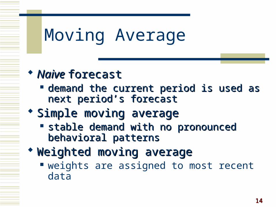
Moving Average

Naive Naive forecastforecast demand the current period is used as next demand the current period is used as next

period’s forecastperiod’s forecast Simple moving averageSimple moving average

stable demand with no pronounced stable demand with no pronounced behavioral patternsbehavioral patterns

Weighted moving averageWeighted moving average weights are assigned to most recent data

1515

Moving Average:Moving Average:Naïve ApproachNaïve Approach

JanJan 120120FebFeb 9090MarMar 100100AprApr 7575MayMay 110110JuneJune 5050JulyJuly 7575AugAug 130130SeptSept 110110OctOct 9090

ORDERSORDERSMONTHMONTH PER MONTHPER MONTH

--120120

9090100100

7575110110

50507575

130130110110

9090Nov -Nov -

FORECASTFORECAST

1616

Simple Moving Average Simple Moving Average

MAMAnn = =

nn

ii = 1= 1 DDii

nnwherewhere

nn ==number of periods number of periods in the moving in the moving

averageaverageDDii ==demand in period demand in period ii

1717

3-month Simple Moving Average3-month Simple Moving Average

JanJan 120120

FebFeb 9090

MarMar 100100

AprApr 7575

MayMay 110110

JuneJune 5050

JulyJuly 7575

AugAug 130130

SeptSept 110110

OctOct 9090NovNov --

ORDERSORDERS

MONTHMONTH PER PER MONTHMONTH

MAMA33 = =

33

ii = 1= 1 DDii

33

==90 + 110 + 13090 + 110 + 130

33

= 110 orders= 110 ordersfor Novfor Nov

––––––

103.3103.388.388.395.095.078.378.378.378.385.085.0

105.0105.0110.0110.0

MOVING MOVING AVERAGEAVERAGE

1818

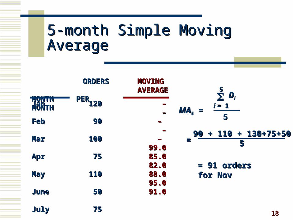
5-month Simple Moving Average5-month Simple Moving Average

JanJan 120120

FebFeb 9090

MarMar 100100

AprApr 7575

MayMay 110110

JuneJune 5050

JulyJuly 7575

AugAug 130130

SeptSept 110110

OctOct 9090NovNov --

ORDERSORDERS

MONTHMONTH PER PER MONTHMONTH MAMA55 = =

55

ii = 1= 1 DDii

55

==90 + 110 + 130+75+5090 + 110 + 130+75+50

55

= 91 orders= 91 ordersfor Novfor Nov

––––

– – ––

– – 99.099.085.085.082.082.088.088.095.095.091.091.0

MOVING MOVING AVERAGEAVERAGE

1919

Smoothing EffectsSmoothing Effects

150 150 –

125 125 –

100 100 –

75 75 –

50 50 –

25 25 –

0 0 –| | | | | | | | | | |

JanJan FebFeb MarMar AprApr MayMay JuneJune JulyJuly AugAug SeptSept OctOct NovNov

ActualActual

Ord

ers

Ord

ers

MonthMonth

5-month5-month

3-month3-month

2020

Weighted Moving AverageWeighted Moving Average

WMAWMAnn = = ii = 1 = 1 WWii D Dii

wherewhere

WWii = the weight for period = the weight for period ii, ,

between 0 and 100 between 0 and 100 percentpercent

WWii = 1.00= 1.00

Adjusts Adjusts moving moving average average method to method to more closely more closely reflect data reflect data fluctuationsfluctuations

2121

Weighted Moving Average ExampleWeighted Moving Average Example

MONTH MONTH WEIGHT WEIGHT DATADATA

AugustAugust 17%17% 130130SeptemberSeptember 33%33% 110110OctoberOctober 50%50% 9090

WMAWMA33 = = 33

ii = 1 = 1 WWii D Dii

= (0.50)(90) + (0.33)(110) + (0.17)(130)= (0.50)(90) + (0.33)(110) + (0.17)(130)

= 103.4 orders= 103.4 orders

November ForecastNovember Forecast

2222

Averaging method Averaging method Weights most recent data more stronglyWeights most recent data more strongly Reacts more to recent changesReacts more to recent changes Widely used, accurate methodWidely used, accurate method

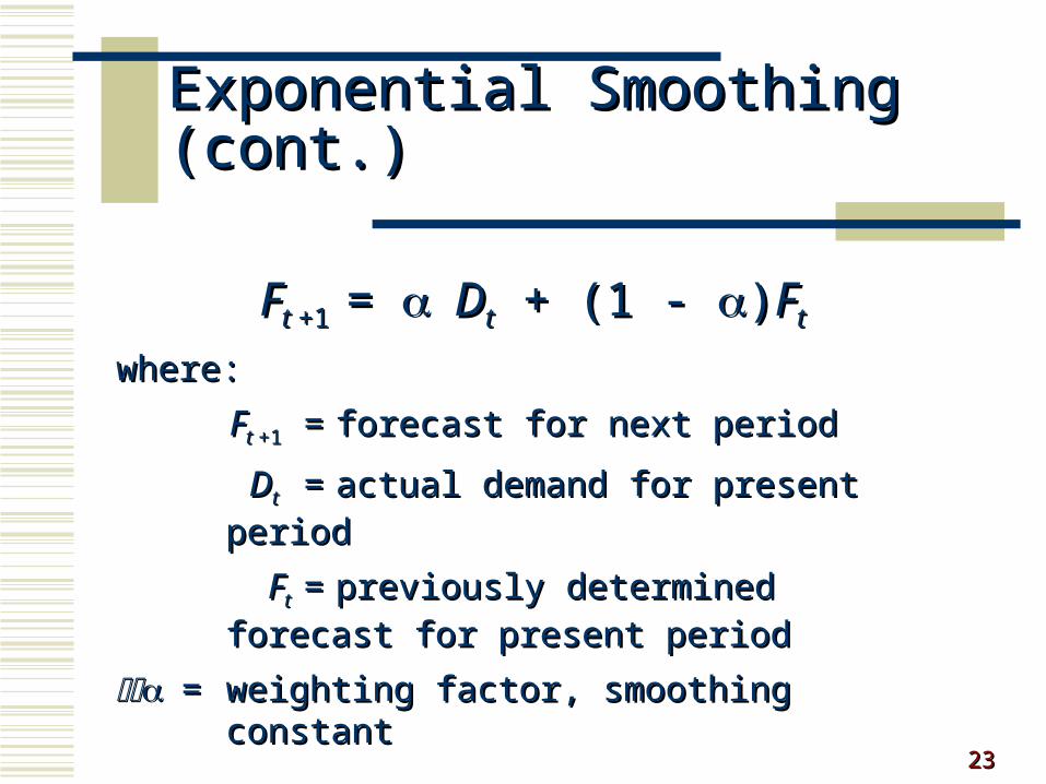
Exponential SmoothingExponential Smoothing

2323

FFt t +1 +1 = = DDtt + (1 - + (1 - ))FFtt

where:where:

FFt t +1+1 = = forecast for next periodforecast for next period

DDtt == actual demand for present periodactual demand for present period

FFtt == previously determined forecast for previously determined forecast for

present periodpresent period

== weighting factor, smoothing constantweighting factor, smoothing constant

Exponential Smoothing (cont.)Exponential Smoothing (cont.)

2424

Effect of Smoothing ConstantEffect of Smoothing Constant

0.0 0.0 1.0 1.0

If If = 0.20, then = 0.20, then FFt t +1 +1 = 0.20= 0.20DDtt + 0.80 + 0.80 FFtt

If If = 0, then = 0, then FFtt +1 +1 = 0= 0DDtt + 1 + 1 FFtt 0 = 0 = FFtt

Forecast does not reflect recent dataForecast does not reflect recent data

If If = 1, then = 1, then FFt t +1 +1 = 1= 1DDtt + 0 + 0 FFtt ==DDtt Forecast based only on most recent dataForecast based only on most recent data

2525

FF22 = = DD11 + (1 - + (1 - ))FF11

= (0.30)(37) + (0.70)(37)= (0.30)(37) + (0.70)(37)

= 37= 37

FF33 = = DD22 + (1 - + (1 - ))FF22

= (0.30)(40) + (0.70)(37)= (0.30)(40) + (0.70)(37)

= 37.9= 37.9

FF1313 = = DD1212 + (1 - + (1 - ))FF1212

= (0.30)(54) + (0.70)(50.84)= (0.30)(54) + (0.70)(50.84)

= 51.79= 51.79

Exponential Smoothing (Exponential Smoothing (αα=0.30)=0.30)

PERIODPERIOD MONTHMONTHDEMANDDEMAND

11 JanJan 3737

22 FebFeb 4040

33 MarMar 4141

44 AprApr 3737

55 May May 4545

66 JunJun 5050

77 Jul Jul 4343

88 Aug Aug 4747

99 Sep Sep 5656

1010 OctOct 5252

1111 NovNov 5555

1212 Dec Dec 5454

2626

FORECAST, FORECAST, FFtt + 1 + 1

PERIODPERIOD MONTHMONTH DEMANDDEMAND (( = 0.3) = 0.3) (( = 0.5) = 0.5)

11 JanJan 3737 –– ––22 FebFeb 4040 37.0037.00 37.0037.0033 MarMar 4141 37.9037.90 38.5038.5044 AprApr 3737 38.8338.83 39.7539.7555 May May 4545 38.2838.28 38.3738.3766 JunJun 5050 40.2940.29 41.6841.6877 Jul Jul 4343 43.2043.20 45.8445.8488 Aug Aug 4747 43.1443.14 44.4244.4299 Sep Sep 5656 44.3044.30 45.7145.71

1010 OctOct 5252 47.8147.81 50.8550.851111 NovNov 5555 49.0649.06 51.4251.421212 Dec Dec 5454 50.8450.84 53.2153.211313 JanJan –– 51.7951.79 53.6153.61

Exponential Smoothing Exponential Smoothing (cont.)(cont.)

2727

70 70 –

60 60 –

50 50 –

40 40 –

30 30 –

20 20 –

1010 –

0 0 –| | | | | | | | | | | | |11 22 33 44 55 66 77 88 99 1010 1111 1212 1313

ActualActual

Ord

ers

Ord

ers

MonthMonth

Exponential Smoothing (cont.)Exponential Smoothing (cont.)

= 0.50= 0.50

= 0.30= 0.30

2828

yy = = aa + + bxbx

wherewherea a = intercept= interceptb b = slope of the line= slope of the linex x = time period= time periody y = forecast for = forecast for demand for period demand for period xx

Linear Trend LineLinear Trend Line

b =

a = y - b x

wheren = number of periods

x = = mean of the x values

y = = mean of the y values

xy - nxy

x2 - nx2

xn

yn

2929

Least Squares ExampleLeast Squares Example

xx(PERIOD)(PERIOD) yy(DEMAND)(DEMAND) xyxy xx22

11 7373 3737 1122 4040 8080 4433 4141 123123 9944 3737 148148 161655 4545 225225 252566 5050 300300 363677 4343 301301 494988 4747 376376 646499 5656 504504 8181

1010 5252 520520 1001001111 5555 605605 1211211212 5454 648648 144144

7878 557557 38673867 650650

3030

x = = 6.5

y = = 46.42

b = = =1.72

a = y - bx= 46.42 - (1.72)(6.5) = 35.2

3867 - (12)(6.5)(46.42)650 - 12(6.5)2

xy - nxyx2 - nx2

781255712

Least Squares Example Least Squares Example (cont.)(cont.)

3131

Linear trend line y = 35.2 + 1.72x

Forecast for period 13 y = 35.2 + 1.72(13) = 57.56 units

70 70 –

60 60 –

50 50 –

40 40 –

30 30 –

20 20 –

1010 –

0 0 –

| | | | | | | | | | | | |11 22 33 44 55 66 77 88 99 1010 1111 1212 1313

ActualActual

Dem

and

Dem

and

PeriodPeriod

Linear trend lineLinear trend line

3232

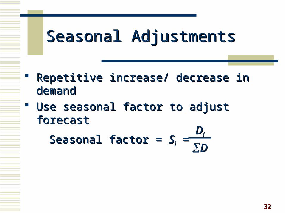
Seasonal AdjustmentsSeasonal Adjustments

Repetitive increase/ decrease in demandRepetitive increase/ decrease in demand Use seasonal factor to adjust forecastUse seasonal factor to adjust forecast

Seasonal factor = Seasonal factor = SSii = =DDii

DD

3333

Seasonal Adjustment (cont.)Seasonal Adjustment (cont.)

2002 12.62002 12.6 8.68.6 6.36.3 17.517.5 45.045.0

2003 14.12003 14.1 10.310.3 7.57.5 18.218.2 50.150.1

2004 15.32004 15.3 10.610.6 8.18.1 19.619.6 53.653.6

Total 42.0Total 42.0 29.529.5 21.921.9 55.355.3 148.7148.7

DEMAND (1000’S PER QUARTER)DEMAND (1000’S PER QUARTER)

YEARYEAR 11 22 33 44 TotalTotal

SS11 = = = 0.28 = = = 0.28 DD11

DD

42.042.0148.7148.7

SS22 = = = 0.20 = = = 0.20 DD22

DD

29.529.5148.7148.7

SS44 = = = 0.37 = = = 0.37 DD44

DD

55.355.3148.7148.7

SS33 = = = 0.15 = = = 0.15 DD33

DD

21.921.9148.7148.7

3434

Seasonal Adjustment (cont.)Seasonal Adjustment (cont.)

SFSF1 1 = (= (SS11) () (FF55) = (0.28)(58.17) = 16.28) = (0.28)(58.17) = 16.28

SFSF2 2 = (= (SS22) () (FF55) = (0.20)(58.17) = 11.63) = (0.20)(58.17) = 11.63

SFSF3 3 = (= (SS33) () (FF55) = (0.15)(58.17) = 8.73) = (0.15)(58.17) = 8.73

SFSF4 4 = (= (SS44) () (FF55) = (0.37)(58.17) = 21.53) = (0.37)(58.17) = 21.53

yy = 40.97 + 4.30= 40.97 + 4.30x x = 40.97 + 4.30(4) = 58.17= 40.97 + 4.30(4) = 58.17

For 2005For 2005

3535

Forecast AccuracyForecast Accuracy

Forecast error difference between forecast and actual demand MAD

mean absolute deviation MAPD

mean absolute percent deviation Cumulative error Average error or bias

3636

Mean Absolute Deviation Mean Absolute Deviation (MAD)(MAD)

wherewhere tt = period number= period number

DDtt = demand in period = demand in period tt

FFtt = forecast for period = forecast for period tt

nn = total number of periods= total number of periods= absolute value= absolute value

DDtt - - FFtt nnMAD =MAD =

3737

MAD ExampleMAD Example

11 3737 37.0037.00 –– ––22 4040 37.0037.00 3.003.00 3.003.0033 4141 37.9037.90 3.103.10 3.103.1044 3737 38.8338.83 -1.83-1.83 1.831.8355 4545 38.2838.28 6.726.72 6.726.7266 5050 40.2940.29 9.699.69 9.699.6977 4343 43.2043.20 -0.20-0.20 0.200.2088 4747 43.1443.14 3.863.86 3.863.8699 5656 44.3044.30 11.7011.70 11.7011.70

1010 5252 47.8147.81 4.194.19 4.194.191111 5555 49.0649.06 5.945.94 5.945.941212 5454 50.8450.84 3.153.15 3.153.15

557557 49.3149.31 53.3953.39

PERIODPERIOD DEMAND, DEMAND, DDtt FFtt ( ( =0.3) =0.3) ((DDtt - - FFtt)) | |DDtt - - FFtt||

Dt - Ft nMAD =

=

= 4.85

53.3911

3838

Other Accuracy MeasuresOther Accuracy Measures

Mean absolute percent deviation (MAPD)Mean absolute percent deviation (MAPD)

MAPD =MAPD =|D|Dtt - F - Ftt||

DDtt

Cumulative errorCumulative error

E = E = eett

Average errorAverage error

E =E =eett

nn

3939

Comparison of ForecastsComparison of Forecasts

FORECASTFORECAST MADMAD MAPDMAPD EE ((EE))

Exponential smoothing (Exponential smoothing (= 0.30)= 0.30) 4.854.85 9.6%9.6% 49.3149.31 4.484.48

Exponential smoothing (Exponential smoothing (= 0.50)= 0.50) 4.044.04 8.5%8.5% 33.2133.21 3.023.02

Adjusted exponential smoothingAdjusted exponential smoothing 3.813.81 7.5%7.5% 21.1421.14 1.921.92

((= 0.50, = 0.50, = 0.30)= 0.30)

Linear trend lineLinear trend line 2.292.29 4.9%4.9% –– ––