Economics 310

Lecture 25Univariate Time-Series

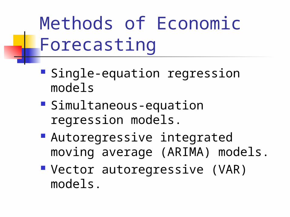
Methods of Economic Forecasting Single-equation regression models Simultaneous-equation regression

models. Autoregressive integrated moving

average (ARIMA) models. Vector autoregressive (VAR)

models.

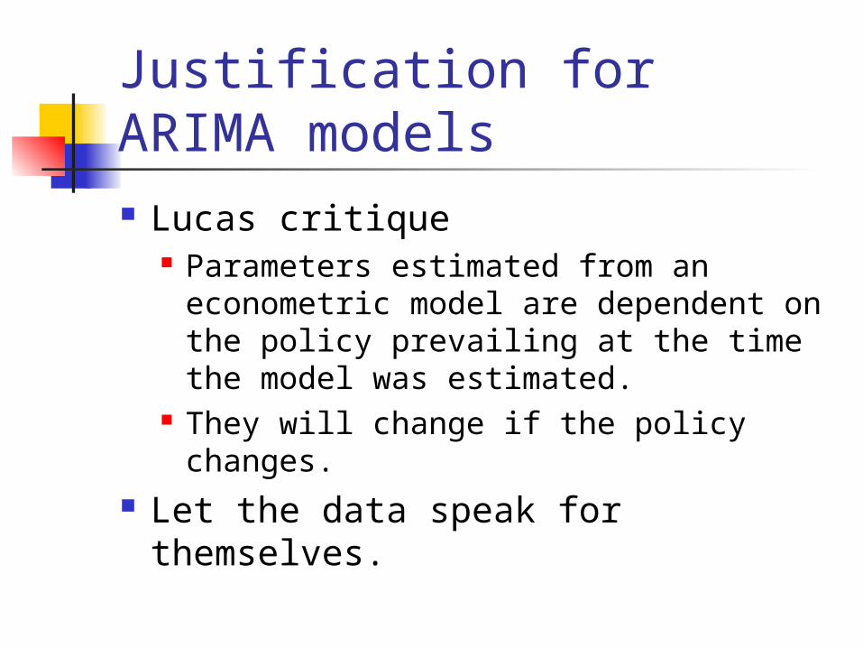
Justification for ARIMA models Lucas critique

Parameters estimated from an econometric model are dependent on the policy prevailing at the time the model was estimated.

They will change if the policy changes.

Let the data speak for themselves.

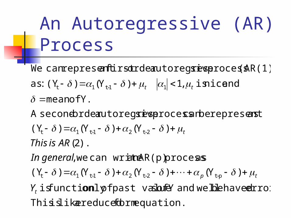
An Autoregressive (AR) Process

equation. form reduced a like is This

error. behaved welland Y of spast value ofonly function is

)Y()Y()Y()(Y

as process AR(p)an can write we,

).2(

)Y()Y()(Y

asrepresent becan process siveautoregresorder -secondA

Y. ofmean

and nice is ,1)Y()(Y :as

(AR(1)) process siveautoregresorder -first arepresent can We

p-t2-t21-t1t

2-t21-t1t

11-t1t

t

tp

t

tt

Y

generalIn

ARisThis

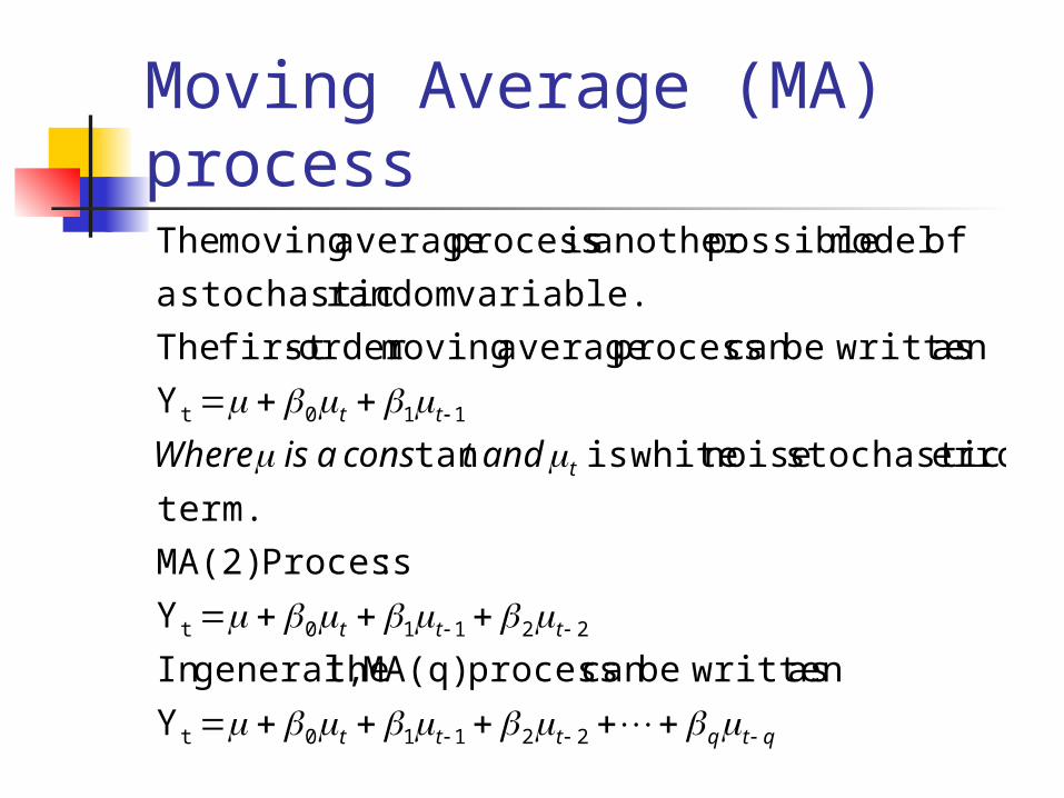
Moving Average (MA) process

qtqttt

ttt

t

tt

andtconsaisWhere

22110t

22110t

110t

Y

as written becan process MA(q) thegeneral,In

Y

:Process MA(2)

term.

error stochastic noise whiteis tan

Y

as written becan process average movingorder -first The

variable.random stochastic a

of model possibleanother is process average moving The

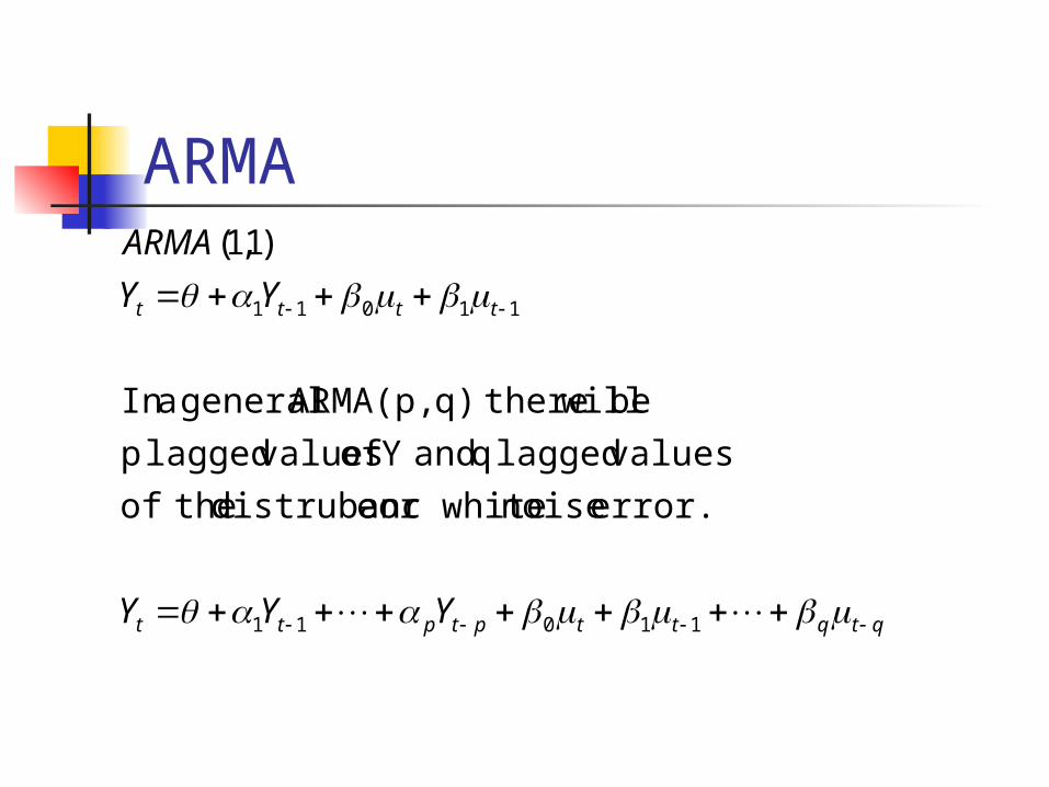
ARMA

qtqttptptt

tttt

YYY

YY

ARMA

11011

11011

error. noise or white edistrubanc theof

valueslagged q and Y of valueslagged p

be will thereq)ARMA(p, general aIn

)1,1(

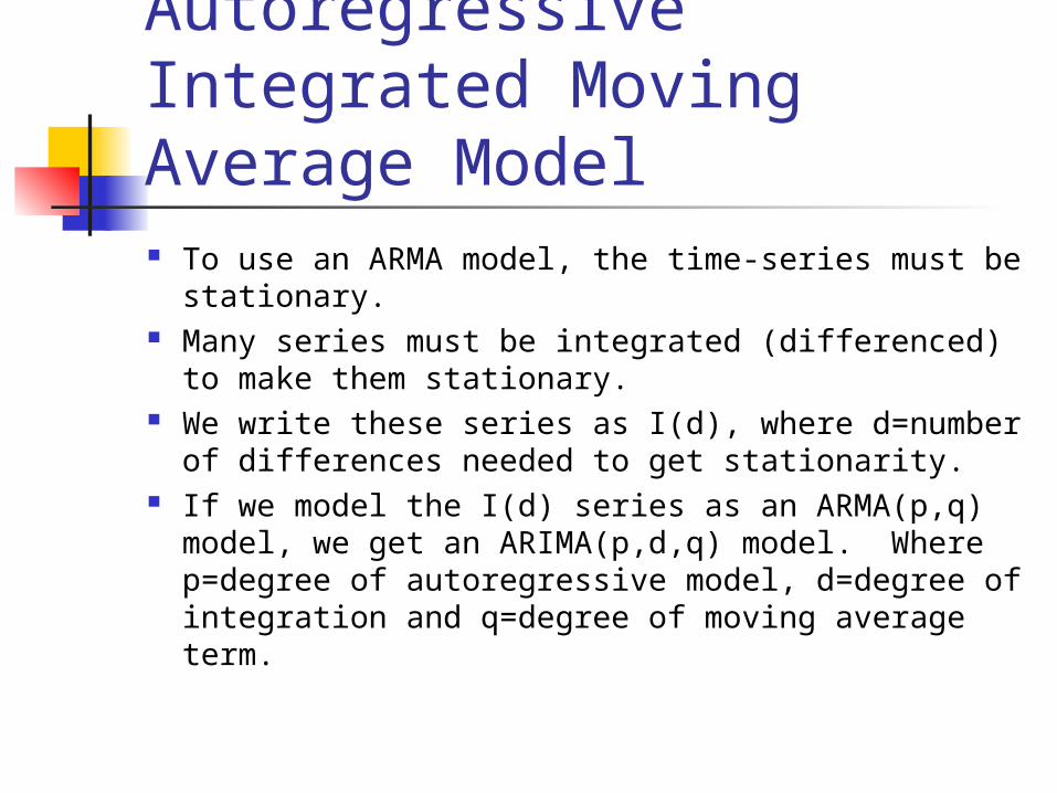
Autoregressive Integrated Moving Average Model To use an ARMA model, the time-series must be

stationary. Many series must be integrated (differenced) to

make them stationary. We write these series as I(d), where d=number

of differences needed to get stationarity. If we model the I(d) series as an ARMA(p,q)

model, we get an ARIMA(p,d,q) model. Where p=degree of autoregressive model, d=degree of integration and q=degree of moving average term.

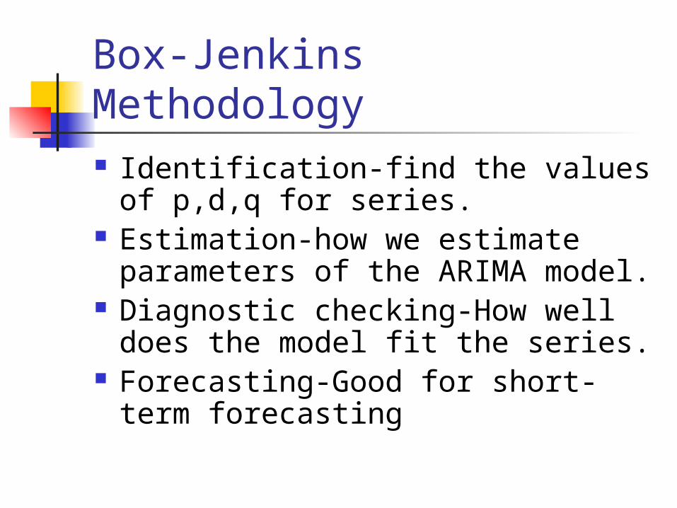
Box-Jenkins Methodology Identification-find the values of

p,d,q for series. Estimation-how we estimate

parameters of the ARIMA model. Diagnostic checking-How well does

the model fit the series. Forecasting-Good for short-term

forecasting

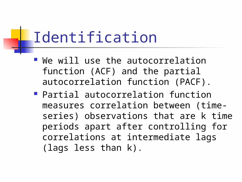
Identification We will use the autocorrelation function

(ACF) and the partial autocorrelation function (PACF).

Partial autocorrelation function measures correlation between (time-series) observations that are k time periods apart after controlling for correlations at intermediate lags (lags less than k).

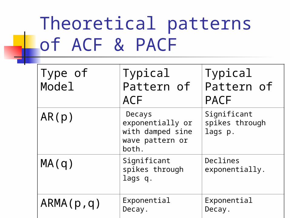
Theoretical patterns of ACF & PACF

Type of Model

Typical Pattern of ACF

Typical Pattern of PACF

AR(p) Decays exponentially or with damped sine wave pattern or both.

Significant spikes through lags p.

MA(q) Significant spikes through lags q.

Declines exponentially.

ARMA(p,q) Exponential Decay. Exponential Decay.

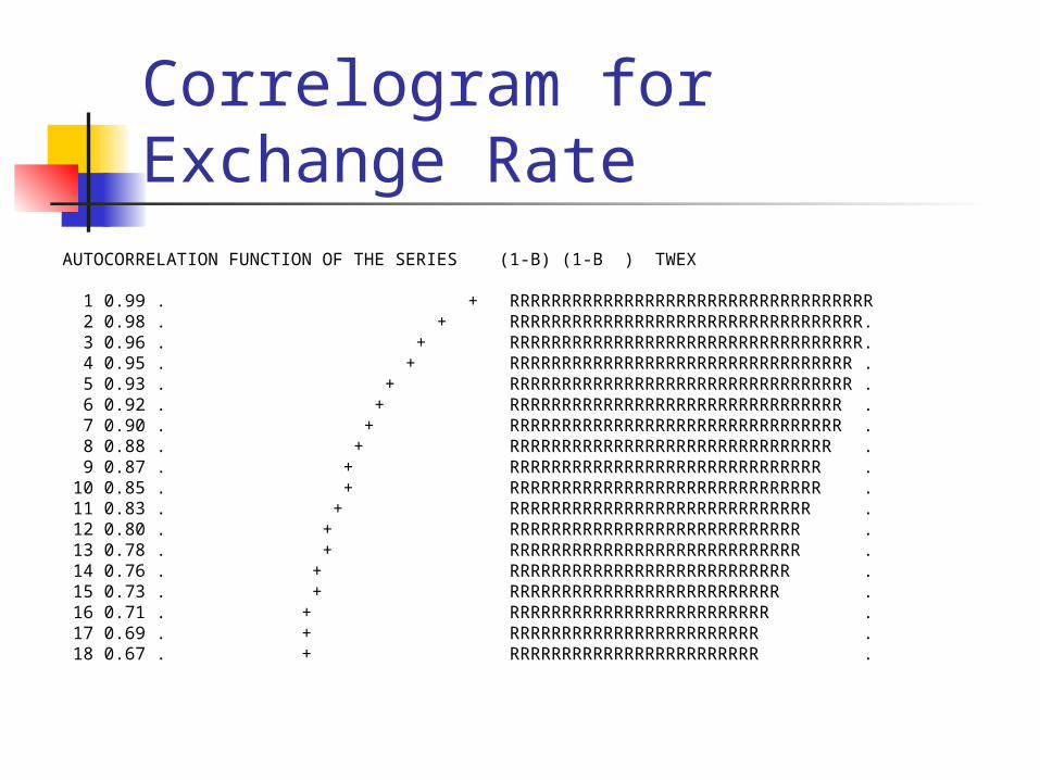
Correlogram for Exchange Rate

AUTOCORRELATION FUNCTION OF THE SERIES (1-B) (1-B ) TWEX 1 0.99 . + RRRRRRRRRRRRRRRRRRRRRRRRRRRRRRRRRRR 2 0.98 . + RRRRRRRRRRRRRRRRRRRRRRRRRRRRRRRRRR. 3 0.96 . + RRRRRRRRRRRRRRRRRRRRRRRRRRRRRRRRRR. 4 0.95 . + RRRRRRRRRRRRRRRRRRRRRRRRRRRRRRRRR . 5 0.93 . + RRRRRRRRRRRRRRRRRRRRRRRRRRRRRRRRR . 6 0.92 . + RRRRRRRRRRRRRRRRRRRRRRRRRRRRRRRR . 7 0.90 . + RRRRRRRRRRRRRRRRRRRRRRRRRRRRRRRR . 8 0.88 . + RRRRRRRRRRRRRRRRRRRRRRRRRRRRRRR . 9 0.87 . + RRRRRRRRRRRRRRRRRRRRRRRRRRRRRR . 10 0.85 . + RRRRRRRRRRRRRRRRRRRRRRRRRRRRRR . 11 0.83 . + RRRRRRRRRRRRRRRRRRRRRRRRRRRRR . 12 0.80 . + RRRRRRRRRRRRRRRRRRRRRRRRRRRR . 13 0.78 . + RRRRRRRRRRRRRRRRRRRRRRRRRRRR . 14 0.76 . + RRRRRRRRRRRRRRRRRRRRRRRRRRR . 15 0.73 . + RRRRRRRRRRRRRRRRRRRRRRRRRR . 16 0.71 . + RRRRRRRRRRRRRRRRRRRRRRRRR . 17 0.69 . + RRRRRRRRRRRRRRRRRRRRRRRR . 18 0.67 . + RRRRRRRRRRRRRRRRRRRRRRRR .

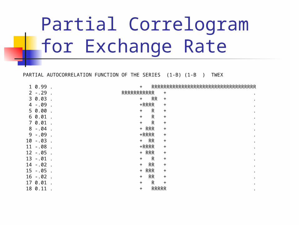
Partial Correlogram for Exchange Rate

PARTIAL AUTOCORRELATION FUNCTION OF THE SERIES (1-B) (1-B ) TWEX 1 0.99 . + RRRRRRRRRRRRRRRRRRRRRRRRRRRRRRRRRRR 2 -.29 . RRRRRRRRRRR + . 3 0.03 . + RR + . 4 -.09 . +RRRR + . 5 0.00 . + R + . 6 0.01 . + R + . 7 0.01 . + R + . 8 -.04 . + RRR + . 9 -.09 . +RRRR + . 10 -.03 . + RR + . 11 -.08 . +RRRR + . 12 -.05 . + RRR + . 13 -.01 . + R + . 14 -.02 . + RR + . 15 -.05 . + RRR + . 16 -.02 . + RR + . 17 0.01 . + R + . 18 0.11 . + RRRRR .

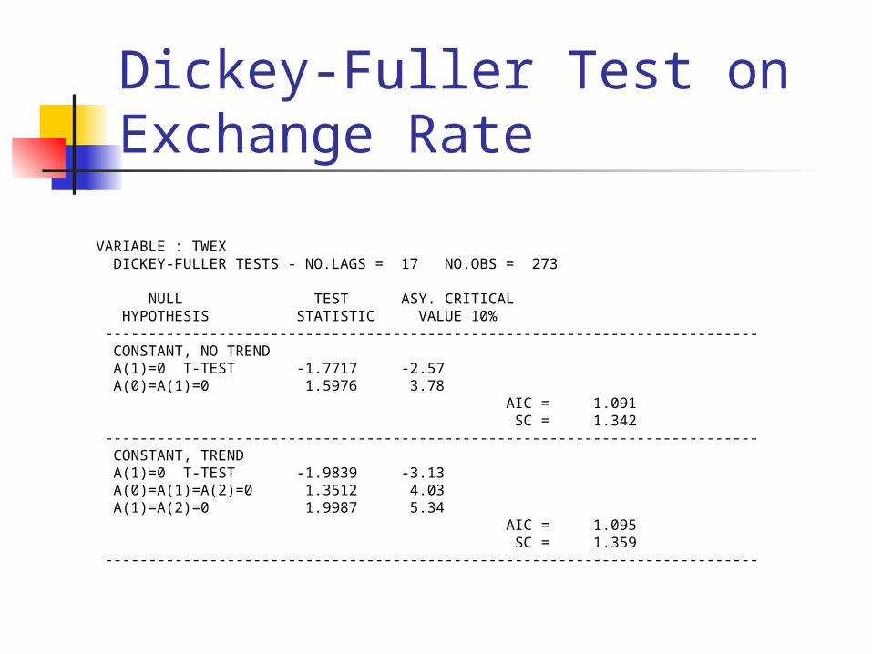
Dickey-Fuller Test on Exchange Rate

VARIABLE : TWEX DICKEY-FULLER TESTS - NO.LAGS = 17 NO.OBS = 273 NULL TEST ASY. CRITICAL HYPOTHESIS STATISTIC VALUE 10% --------------------------------------------------------------------------- CONSTANT, NO TREND A(1)=0 T-TEST -1.7717 -2.57 A(0)=A(1)=0 1.5976 3.78 AIC = 1.091 SC = 1.342 --------------------------------------------------------------------------- CONSTANT, TREND A(1)=0 T-TEST -1.9839 -3.13 A(0)=A(1)=A(2)=0 1.3512 4.03 A(1)=A(2)=0 1.9987 5.34 AIC = 1.095 SC = 1.359 ---------------------------------------------------------------------------

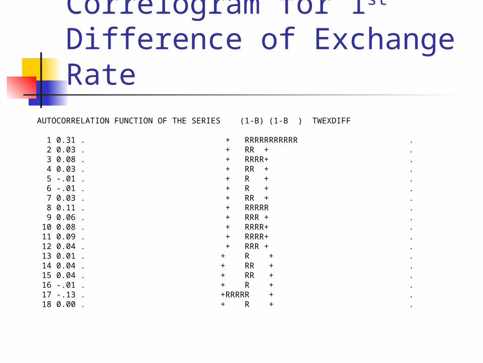
Correlogram for 1st Difference of Exchange Rate

AUTOCORRELATION FUNCTION OF THE SERIES (1-B) (1-B ) TWEXDIFF 1 0.31 . + RRRRRRRRRRR . 2 0.03 . + RR + . 3 0.08 . + RRRR+ . 4 0.03 . + RR + . 5 -.01 . + R + . 6 -.01 . + R + . 7 0.03 . + RR + . 8 0.11 . + RRRRR . 9 0.06 . + RRR + . 10 0.08 . + RRRR+ . 11 0.09 . + RRRR+ . 12 0.04 . + RRR + . 13 0.01 . + R + . 14 0.04 . + RR + . 15 0.04 . + RR + . 16 -.01 . + R + . 17 -.13 . +RRRRR + . 18 0.00 . + R + .

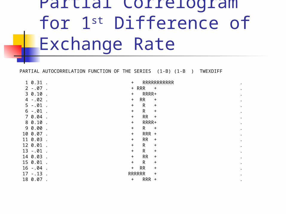
Partial Correlogram for 1st Difference of Exchange Rate

PARTIAL AUTOCORRELATION FUNCTION OF THE SERIES (1-B) (1-B ) TWEXDIFF 1 0.31 . + RRRRRRRRRRR . 2 -.07 . + RRR + . 3 0.10 . + RRRR+ . 4 -.02 . + RR + . 5 -.01 . + R + . 6 -.01 . + R + . 7 0.04 . + RR + . 8 0.10 . + RRRR+ . 9 0.00 . + R + . 10 0.07 . + RRR + . 11 0.03 . + RR + . 12 0.01 . + R + . 13 -.01 . + R + . 14 0.03 . + RR + . 15 0.01 . + R + . 16 -.04 . + RR + . 17 -.13 . RRRRRR + . 18 0.07 . + RRR + .

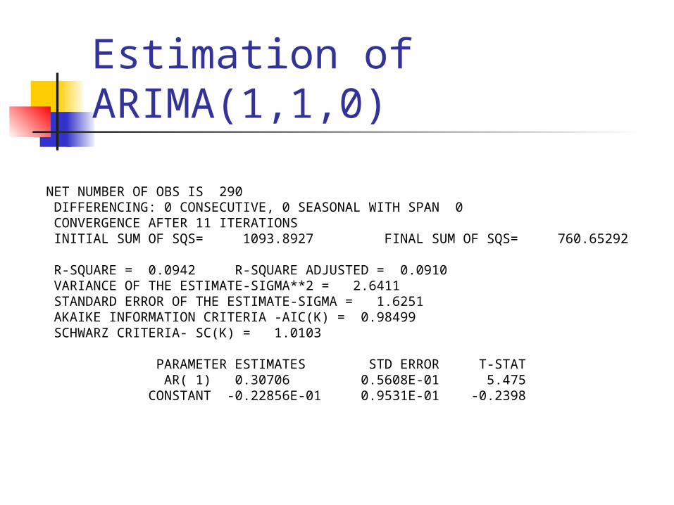
Estimation of ARIMA(1,1,0)

NET NUMBER OF OBS IS 290 DIFFERENCING: 0 CONSECUTIVE, 0 SEASONAL WITH SPAN 0 CONVERGENCE AFTER 11 ITERATIONS INITIAL SUM OF SQS= 1093.8927 FINAL SUM OF SQS= 760.65292 R-SQUARE = 0.0942 R-SQUARE ADJUSTED = 0.0910 VARIANCE OF THE ESTIMATE-SIGMA**2 = 2.6411 STANDARD ERROR OF THE ESTIMATE-SIGMA = 1.6251 AKAIKE INFORMATION CRITERIA -AIC(K) = 0.98499 SCHWARZ CRITERIA- SC(K) = 1.0103 PARAMETER ESTIMATES STD ERROR T-STAT AR( 1) 0.30706 0.5608E-01 5.475 CONSTANT -0.22856E-01 0.9531E-01 -0.2398

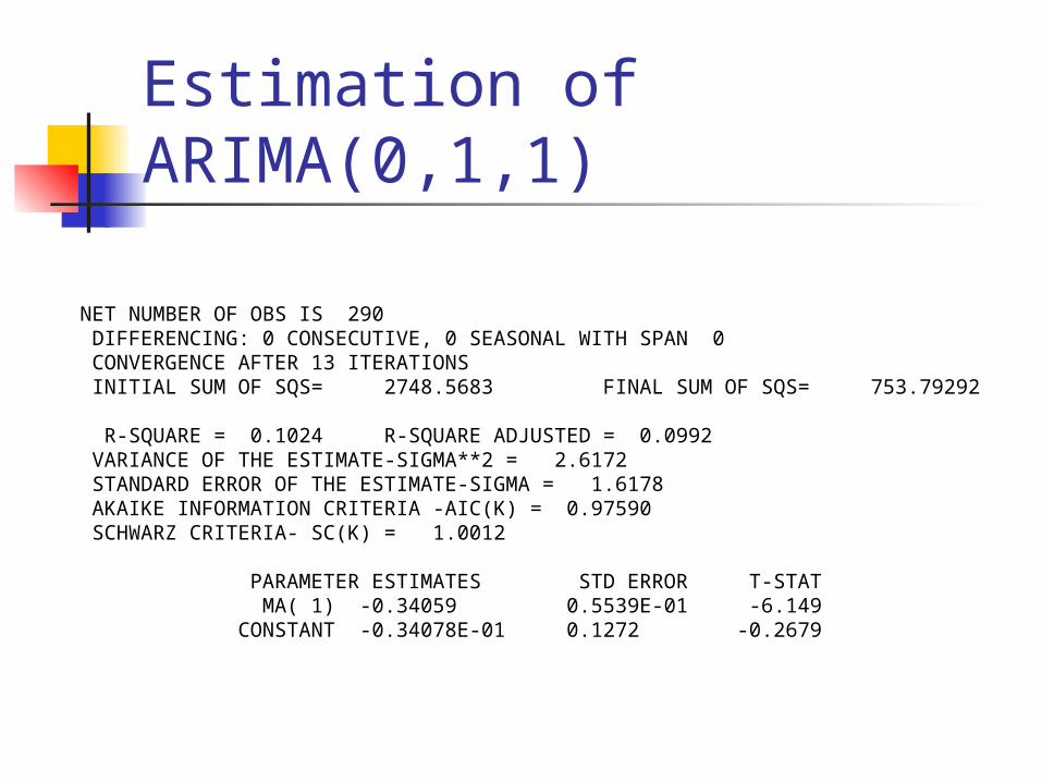
Estimation of ARIMA(0,1,1)

NET NUMBER OF OBS IS 290 DIFFERENCING: 0 CONSECUTIVE, 0 SEASONAL WITH SPAN 0 CONVERGENCE AFTER 13 ITERATIONS INITIAL SUM OF SQS= 2748.5683 FINAL SUM OF SQS= 753.79292 R-SQUARE = 0.1024 R-SQUARE ADJUSTED = 0.0992 VARIANCE OF THE ESTIMATE-SIGMA**2 = 2.6172 STANDARD ERROR OF THE ESTIMATE-SIGMA = 1.6178 AKAIKE INFORMATION CRITERIA -AIC(K) = 0.97590 SCHWARZ CRITERIA- SC(K) = 1.0012 PARAMETER ESTIMATES STD ERROR T-STAT MA( 1) -0.34059 0.5539E-01 -6.149 CONSTANT -0.34078E-01 0.1272 -0.2679

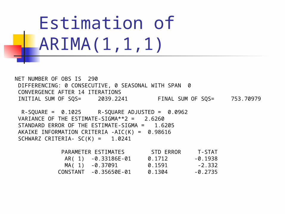
Estimation of ARIMA(1,1,1)

NET NUMBER OF OBS IS 290 DIFFERENCING: 0 CONSECUTIVE, 0 SEASONAL WITH SPAN 0 CONVERGENCE AFTER 14 ITERATIONS INITIAL SUM OF SQS= 2039.2241 FINAL SUM OF SQS= 753.70979 R-SQUARE = 0.1025 R-SQUARE ADJUSTED = 0.0962 VARIANCE OF THE ESTIMATE-SIGMA**2 = 2.6260 STANDARD ERROR OF THE ESTIMATE-SIGMA = 1.6205 AKAIKE INFORMATION CRITERIA -AIC(K) = 0.98616 SCHWARZ CRITERIA- SC(K) = 1.0241 PARAMETER ESTIMATES STD ERROR T-STAT AR( 1) -0.33186E-01 0.1712 -0.1938 MA( 1) -0.37091 0.1591 -2.332 CONSTANT -0.35650E-01 0.1304 -0.2735

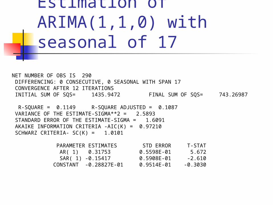
Estimation of ARIMA(1,1,0) with seasonal of 17

NET NUMBER OF OBS IS 290 DIFFERENCING: 0 CONSECUTIVE, 0 SEASONAL WITH SPAN 17 CONVERGENCE AFTER 12 ITERATIONS INITIAL SUM OF SQS= 1435.9472 FINAL SUM OF SQS= 743.26987 R-SQUARE = 0.1149 R-SQUARE ADJUSTED = 0.1087 VARIANCE OF THE ESTIMATE-SIGMA**2 = 2.5893 STANDARD ERROR OF THE ESTIMATE-SIGMA = 1.6091 AKAIKE INFORMATION CRITERIA -AIC(K) = 0.97210 SCHWARZ CRITERIA- SC(K) = 1.0101 PARAMETER ESTIMATES STD ERROR T-STAT AR( 1) 0.31753 0.5598E-01 5.672 SAR( 1) -0.15417 0.5908E-01 -2.610 CONSTANT -0.28827E-01 0.9514E-01 -0.3030

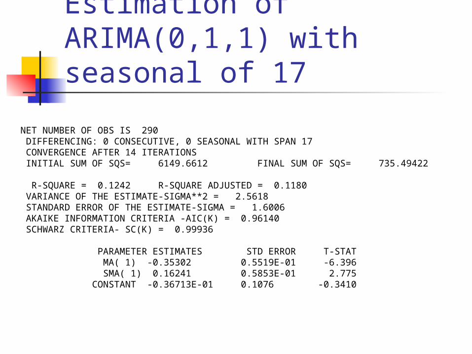
Estimation of ARIMA(0,1,1) with seasonal of 17

NET NUMBER OF OBS IS 290 DIFFERENCING: 0 CONSECUTIVE, 0 SEASONAL WITH SPAN 17 CONVERGENCE AFTER 14 ITERATIONS INITIAL SUM OF SQS= 6149.6612 FINAL SUM OF SQS= 735.49422 R-SQUARE = 0.1242 R-SQUARE ADJUSTED = 0.1180 VARIANCE OF THE ESTIMATE-SIGMA**2 = 2.5618 STANDARD ERROR OF THE ESTIMATE-SIGMA = 1.6006 AKAIKE INFORMATION CRITERIA -AIC(K) = 0.96140 SCHWARZ CRITERIA- SC(K) = 0.99936 PARAMETER ESTIMATES STD ERROR T-STAT MA( 1) -0.35302 0.5519E-01 -6.396 SMA( 1) 0.16241 0.5853E-01 2.775 CONSTANT -0.36713E-01 0.1076 -0.3410

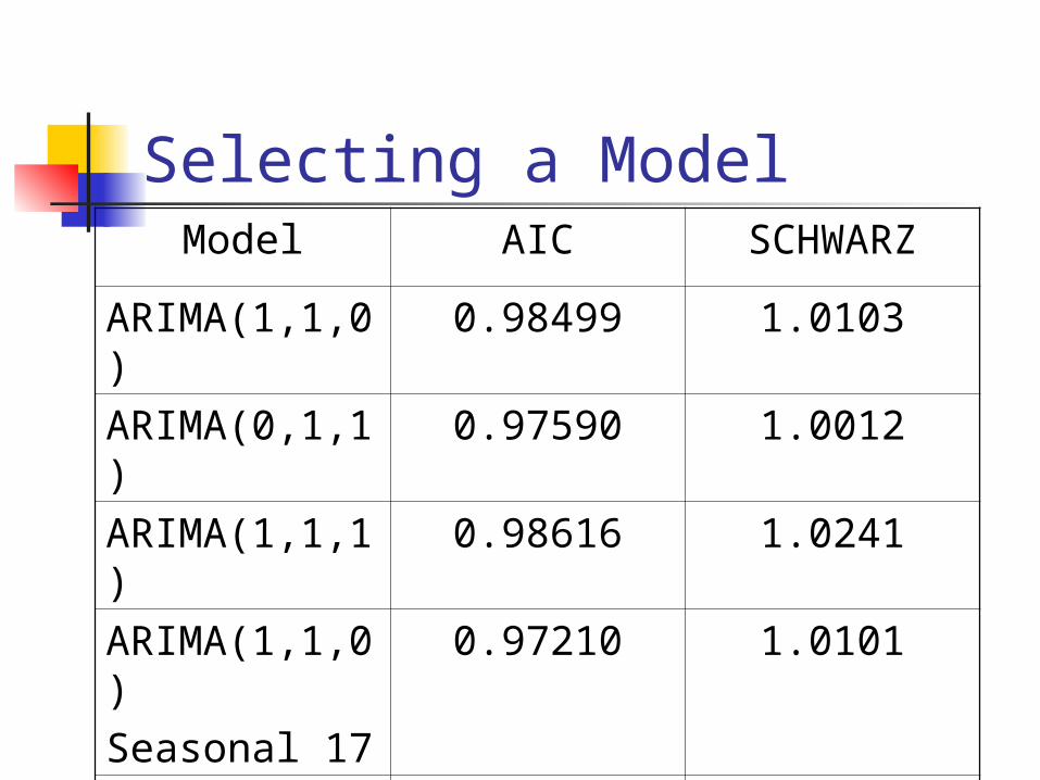
Selecting a ModelModel AIC SCHWARZ

ARIMA(1,1,0) 0.98499 1.0103

ARIMA(0,1,1) 0.97590 1.0012

ARIMA(1,1,1) 0.98616 1.0241

ARIMA(1,1,0)Seasonal 17

0.97210 1.0101

ARIMA(0,1,1)Seasonal 17

0.96140 0.99936

Diagnostic We want to check the adequacy of our

model. For an ARIMA(p,d,q), check that the

added coefficients for ARIMA(p+1,d,q) and ARIMA(p,d,q+1) are zero.

Do a plot of the autocorrelation of residuals from the model to see that they are white noise.

Run a Ljung-Box test on the residuals to see that they are White noise.

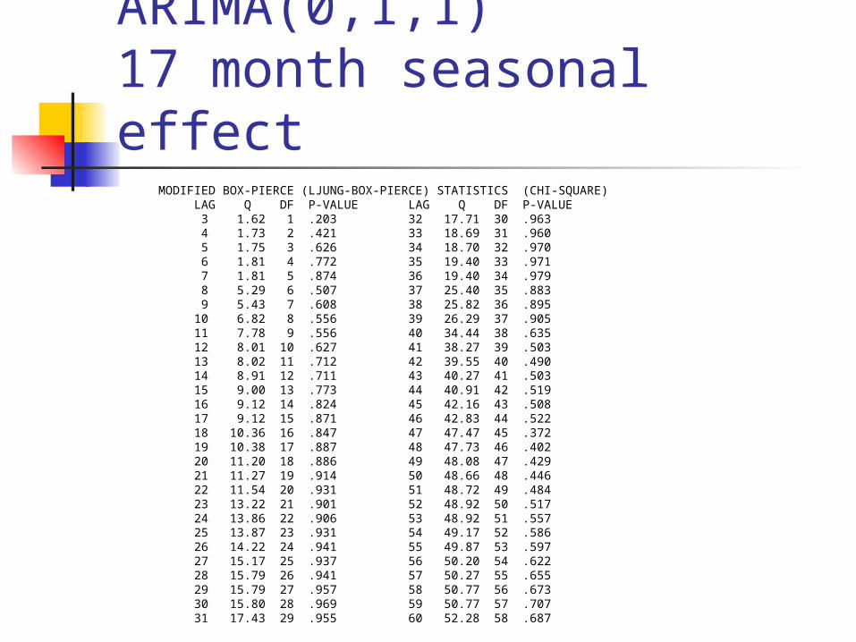
Diagnostics-ARIMA(0,1,1)17 month seasonal effect

MODIFIED BOX-PIERCE (LJUNG-BOX-PIERCE) STATISTICS (CHI-SQUARE) LAG Q DF P-VALUE LAG Q DF P-VALUE 3 1.62 1 .203 32 17.71 30 .963 4 1.73 2 .421 33 18.69 31 .960 5 1.75 3 .626 34 18.70 32 .970 6 1.81 4 .772 35 19.40 33 .971 7 1.81 5 .874 36 19.40 34 .979 8 5.29 6 .507 37 25.40 35 .883 9 5.43 7 .608 38 25.82 36 .895 10 6.82 8 .556 39 26.29 37 .905 11 7.78 9 .556 40 34.44 38 .635 12 8.01 10 .627 41 38.27 39 .503 13 8.02 11 .712 42 39.55 40 .490 14 8.91 12 .711 43 40.27 41 .503 15 9.00 13 .773 44 40.91 42 .519 16 9.12 14 .824 45 42.16 43 .508 17 9.12 15 .871 46 42.83 44 .522 18 10.36 16 .847 47 47.47 45 .372 19 10.38 17 .887 48 47.73 46 .402 20 11.20 18 .886 49 48.08 47 .429 21 11.27 19 .914 50 48.66 48 .446 22 11.54 20 .931 51 48.72 49 .484 23 13.22 21 .901 52 48.92 50 .517 24 13.86 22 .906 53 48.92 51 .557 25 13.87 23 .931 54 49.17 52 .586 26 14.22 24 .941 55 49.87 53 .597 27 15.17 25 .937 56 50.20 54 .622 28 15.79 26 .941 57 50.27 55 .655 29 15.79 27 .957 58 50.77 56 .673 30 15.80 28 .969 59 50.77 57 .707 31 17.43 29 .955 60 52.28 58 .687

Diagnostics-ARIMA(0,1,1)17 month seasonal effect

RESIDUALS LAGS AUTOCORRELATIONS STD ERR 1 -12 0.00 0.02 0.07 0.02 -.01 0.01 0.01 0.11 0.02 0.07 0.06 0.03 0.06 13 -24 0.00 0.05 0.02 0.02 0.00 0.06 -.01 -.05 0.02 0.03 0.07 -.04 0.06 25 -36 0.01 -.03 0.05 -.04 0.00 0.00 0.07 -.03 -.05 0.00 0.05 0.00 0.06 37 -48 -.13 -.04 -.04 -.16 0.11 -.06 0.05 -.04 0.06 -.04 -.12 -.03 0.06 49 -60 -.03 -.04 0.01 -.02 0.00 0.03 -.04 -.03 -.01 -.04 0.00 -.06 0.07

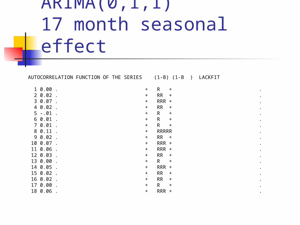
Diagnostics-ARIMA(0,1,1)17 month seasonal effect

AUTOCORRELATION FUNCTION OF THE SERIES (1-B) (1-B ) LACKFIT 1 0.00 . + R + . 2 0.02 . + RR + . 3 0.07 . + RRR + . 4 0.02 . + RR + . 5 -.01 . + R + . 6 0.01 . + R + . 7 0.01 . + R + . 8 0.11 . + RRRRR . 9 0.02 . + RR + . 10 0.07 . + RRR + . 11 0.06 . + RRR + . 12 0.03 . + RR + . 13 0.00 . + R + . 14 0.05 . + RRR + . 15 0.02 . + RR + . 16 0.02 . + RR + . 17 0.00 . + R + . 18 0.06 . + RRR + .

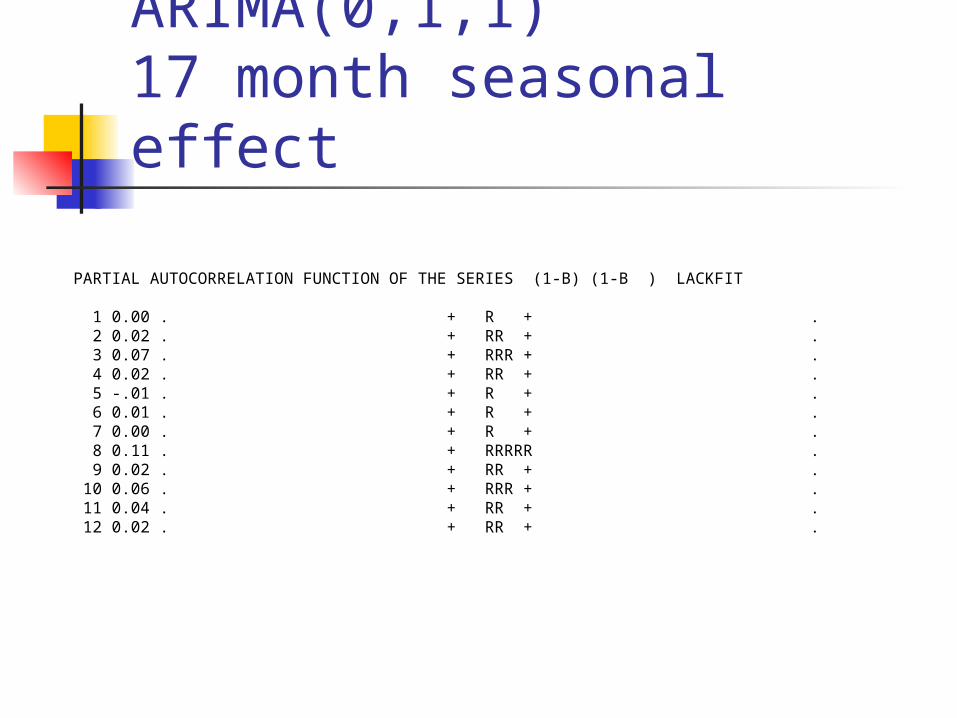
Diagnostics-ARIMA(0,1,1)17 month seasonal effect

PARTIAL AUTOCORRELATION FUNCTION OF THE SERIES (1-B) (1-B ) LACKFIT 1 0.00 . + R + . 2 0.02 . + RR + . 3 0.07 . + RRR + . 4 0.02 . + RR + . 5 -.01 . + R + . 6 0.01 . + R + . 7 0.00 . + R + . 8 0.11 . + RRRRR . 9 0.02 . + RR + . 10 0.06 . + RRR + . 11 0.04 . + RR + . 12 0.02 . + RR + .

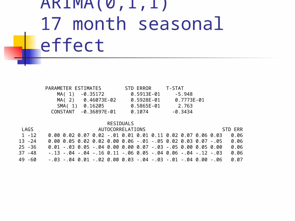
Diagnostics-ARIMA(0,1,1)17 month seasonal effect

PARAMETER ESTIMATES STD ERROR T-STAT MA( 1) -0.35172 0.5913E-01 -5.948 MA( 2) 0.46073E-02 0.5928E-01 0.7773E-01 SMA( 1) 0.16205 0.5865E-01 2.763 CONSTANT -0.36897E-01 0.1074 -0.3434 RESIDUALS LAGS AUTOCORRELATIONS STD ERR 1 -12 0.00 0.02 0.07 0.02 -.01 0.01 0.01 0.11 0.02 0.07 0.06 0.03 0.06 13 -24 0.00 0.05 0.02 0.02 0.00 0.06 -.01 -.05 0.02 0.03 0.07 -.05 0.06 25 -36 0.01 -.03 0.05 -.04 0.00 0.00 0.07 -.03 -.05 0.00 0.05 0.00 0.06 37 -48 -.13 -.04 -.04 -.16 0.11 -.06 0.05 -.04 0.06 -.04 -.12 -.03 0.06 49 -60 -.03 -.04 0.01 -.02 0.00 0.03 -.04 -.03 -.01 -.04 0.00 -.06 0.07