OPERATIONAL RESEARCH AND QUANTITATIVE METHODS IN MANAGEMENT 1140

APPLICATION OF SOME LOCATIONAL MODELS IN NATURAL RESOURCES INDUSTRY - AGRICULTURE CASE 1141

Andrić Gušavac Bisera, Stojanović Dragana, Sokolović Ţeljko

MULTIPLE CRITERIA APPROACH TO SELECTING SITES FOR PORTS OF NAUTICAL TOURISM 1149

Kovaĉić Mirjana, Jugović Alen, Perić Hadţić Ana

TRAVEL BEHAVIOUR OF TEENAGERS: KEY ATTRIBUTES IN CHOOSING TOURIST OFFER 1157

Vukic Milena, Kuzmanovic Marija, Kostić - Stanković Milica

PREFERENCES TOWARDS ORGANIC VS. NON-ORGANIC FOOD: AN EMPIRICAL STUDY OF CONSUMERS IN SERBIA 1165

Marinovic Minja, Popovic Milena, Kuzmanovic Marija

MATHEMATICAL MODEL OF OPTIMAL ECONOMIC PLAN FOOD FOR LUNCH MEMBERS OF SERBIAN ARMY 1172

Jovic Sasa, Tesanovic Branko, Tešanović Jelena

INVENTORY MODEL FOR DIFFERENT KIND OF PRODUCTS - THE CAPACITY OF STORAGE SPACE AS A CONSTRAINING FACTOR 1180

Vasileva Liljana, Atanasova-Pachemska Tatjana, Pachemska Sanja

OPTIMAL VEHICLE ROUTING IN THE OIL INDUSTRY 1186

Golubovic Jelena, Makajić-Nikolić Dragana, Nikolić Nebojša

EFFECTIVENESS DETERMINATION OF HIGHER EDUCATION USING LINEAR PROGRAMMING 1192

Timovski Riste, Atanasova-Paĉemska Tatjana

MULTI-CRITERIA OPTIMIZATION OF THE MOST COMPETITIVE BANK IN MONTENEGRO SELECTION PROCESS 1199

Rakocevic Svetlana, Dragašević Zdenka, Glišević Nevenka

RISK MANAGEMENT IN OPERATIONAL PLANNING PROCESS AT THE OPERATIONAL AND TACTICAL LEVELS 1207

Karovic Samed, Radovanovic Goran, Ristić Vladimir

A NEW CONSTRUCTIVE HEURISTICS FOR SOLVING THE MINIMUM FEEDBACK VERTEX SET PROBLEM1216

Stanojević Milan, Stanojevic Bogdana

OPERATIONAL RESEARCH AND QUANTITATIVE METHODS IN

MANAGEMENT

1140

APPLICATION OF SOME LOCATIONAL MODELS IN NATURAL RESOURCES INDUSTRY - AGRICULTURE CASE

Bisera Andrić Gušavac1, Dragana Stojanović1, Željko Sokolović2

1University of Belgrade, Faculty of Organizational Sciences, {bisera; stojanovicd}@fon.bg.ac.rs 2Railroad Technician School, zex.sokolovic@gmail.com

Abstract: Nowadays large scale, uncertainty and multiple objectives appear increasingly in decision processes. One of the very important strategic decision for starting a business is where to locate facility. Application of operations research methods and models has had a great success throughout the years, including modeling and solving various location problems. Natural resources industry, especially agriculture sector, is a significant factor of growth and prosperity most commonly for developing countries. Operations research/management science (OR/MS) contributions in each one of applied areas of natural resource industry – agriculture, fisheries, forestry and mining are very significant. In this paper we present application of Capacitated Facility Location Problem (CFLP) in agriculture sector and we are encouraging researchers to use quantitative techniques in order to manage the use of different natural resources.

Keywords: Natural resources industry, Agriculture sector, Location analysis, Capacitated FLP

1. INTRODUCTION

By using natural resources according to their needs, a man survived and evolved as a cultural, social and spiritual being. The development of various technologies shaped the life of modern man, but led to the rapid exploitation of its environment, and the rapid depletion of resources. People have changed the face of the earth more than any other species in the history of the planet - and the speed of these changes is increasing. People today spend between one-third and one-half of what the global ecosystem created.

The natural resources of a country determine its wealth and status in the world economic system, its power and political influence. According to this, it is obvious that operations research, as a discipline that deals with the application of advanced analytical methods to help make better decisions has a significant impact on decisions in this area. Application of operational research methods and models to modelling of complex realities and development of algorithms for problems increasingly difficult to solve has had a great success throughout the years (Weintraub, 2007).

Operations research has played an important role in the analysis and decision making of natural resources, specifically, in agriculture, fisheries, forestry and mining, in the last 40 years (Weintraub, 2007). There are natural differences related to the form of managing the production in each application. For example, the time horizons of growth and extraction vary from months to a year for fisheries and agriculture, to almost a century for some tree species. Mining is non-renewable, and, as such, is associated with a different type of natural resource (Bjørndal et al., 2012). Mine lives can run for a few years to centuries. In agriculture, farmers are primarily concerned with how to plant crops and raise animals more efficiently.

Decisions in forestry are centered around the strategic, tactical and operational levels of managing plantations and public lands to meet demands while adhering to supply restrictions, which are coupled with events such as forest fires and policies, e.g., environmental regulations and concerns (Bjørndal, 2012).

Operations research, e.g. location analysis has been applied to handle various problems in agriculture and forestry area, elaborating on mathematical techniques and successful applications. In this paper we present one more application of OR/MS in agriculture sector and we are encouraging researchers to use quantitative techniques in order to manage the use of different natural resources efficiently from an economic as well as an environmental point of view.

2. NATURAL RESOURCES INDUSTRY AND OR/MS

According to the significance of natural resources especially today, it would be expected that operations research (OR) could have made a significant contribution to decision making in this area. But achievements in practice have been disappointingly small. The industry comprises of a large number of small individual businesses which do not permit specialisation in management functions. Consequently, technical advice and

1141

much R and D is provided from public funds. OR applications for agriculture have mainly been developed by Universities, Colleges, State Advisory Services and Quangos. Quango is a quasi-autonomous non-governmental organisation is an organisation to which a government has devolved power. In the United Kingdom this term covers different "arm's-length" government bodies, including "non-departmental public bodies", non-ministerial departments, and executive agencies. The Forestry Commission, which is a non-ministerial government department responsible for forestry in England and Scotland, is an example of a quango (Wikipedia, http://en.wikipedia.org/wiki/Quango). Some techniques are frequently used in agriculture like linear programming, dynamic programming and simulation. Other techniques have had limited uptake and application. Reasons for the pretty low impact of OR are outlined as a set of problems specific to farmers and their systems and problems specific to computer use. One of the obvious problems in efficient application of OR/MS methods and techniques are in recruiting and training OR specialists for these specific fields of application. Generally, how important OR models are in decision making depends on several factors (Weintraub & Romero 2006): —The quality of data, —The competitiveness of markets, —Ownership and —The culture of the application area and peoples’ understanding of OR’s advantages. There exists several ways for increasing OR impact in these areas: one is in training today's farmers (and, probably more important, future farmers) in an understanding of what computers can do and what models are available. There is a general lack of good flexible formulation of problems to be dealt with by OR techniques. A third problem is the need for much more efficient two-way communication and feedback between the developers of OR tools for agriculture and practical farmers. At present OR has connotations of being of little use to practical farmers, but of great value to academic enthusiasts who are unable and/or unwilling to transfer ideas into practicality.

3. APPLICATION OF LOCATION MODELS IN AGRICULTURE SECTOR

Location theory has found its use in agriculture since the early days of the field. The theory of spatial equilibrium and optimal location and the foundations of agricultural location theory are traced back to the classical work of von Thunen in 1826. He investigated the impact of the distance from the market on the use of agricultural land. In agriculture, use of OR models is increasing with advances in hardware and software. The most commonly used OR techniques are LP models, simulation, risk programming, and multiple-criteria programming. People use models at two levels and for two purposes. They use them to improve decisions at the farm level, and they use them to help policy makers predict the impact of policy changes on farmers’ behaviour (Weintraub & Romero 2006). Lucas and Chhajed (2004) give an overview of application of location analysis in field of agriculture and some selected applications of location analysis in agriculture are presented in table 1. Table 1: Selected applications of location analysis in agriculture (adapted from Lucas and Chhajed (2004)) Authors Problem description Features

Grain storage in South Brazil (Borstein and de Casto Villela, 1990)

Optimal location of warehouses for grain storage, then location of service stations for technical assistance

Economies of scale Political, economic, and social aspects Partially funded by State Agency

Soybean-processing industry (D. Souza, 1988)

Optimal number, size, and location of soybean processing plants

Large size, with 57 regions US Economies of scale Multi-commodity (soybeans, then meal and oil) Consideration of two base periods 1977-1981 and predictions for 1999 and 2000

Cattle-slaughtering industry in Queensland, Australia (Brown and Drynan, 1986)

Selection of plant sites, sizes, throughputs and product flow

Economies of scale Marked seasonal and year-to-year variations Comparison of results form static and dynamic models

1142

Authors Problem description Features

Post-harvest handling-chain operations in Northern Tahiland (Chu, 1989)

Optimal number and location of cooling facilities and assignment of production sites to those facilities

Large-size problem with 30 villages and 50 kinds of vegetable products, Problem decomposition, based on access road network and on locations of various extension stations Seasonality of production volumes and access road conditions Project supported by Government

Dairy industry in Ontario, Canada (Polley, 1994)

Changes in existing network (closing of several plants and warehouses) at Aults Foods – Canada’s largest diary processor

Analyse the benefits of specializing each plants production mix and using multiple sources for shipping depots Sensitivity analysis with sales projection for 3, 5 and 10 year 30 plant production strategies

Brewing industry in Turkey (Koksalan, 1995)

Optimal locations of new breweries, and optimal distribution plans for malt and beer

Large-scale problem with 15 alternative cites and 300 customer zones High seasonality of beer demand, capacity constraints

Mladenović (2004) states common classification of location problems into (a) continual, (b) discrete, and (c) network models. Location problems in agriculture exhibit several features, such as their large scope and size, or the consideration of multiple and often conflicting objectives and, thus, demonstrate increased levels of complexity and realism. Common in agriculture are location– allocation problems, in which the number of facilities, their locations, and these interactions all become decision variables. Moreover, these location–allocation problems themselves are often complicated by routing decisions, leading to location–allocation-routing models.

Lucas and Chhajed (2004) presents six groups of location analysis application in agriculture: a cotton-ginning problem, the location of grain sub-terminals, the collection and processing of rubber, the fresh citrus packing industry, the cattle-slaughtering industry and The Bangladesh grain model. These applications of location analysis in agriculture do not consider solving of airfield location problems. Description and solution of one of the first problems regarding location models in agriculture aviation in Serbia can be found in Andrić Gušavac et al. 2013.

3.1 Simple and capacitated plant location problems

The simple plant-location problem (SPLP), also known as the uncapacitated facility-location problem, is one of the fundamental and most studied models in facility-location theory. The objective is to choose, from a set of potential facility-locations on a network, which ones to open to minimize the sum of opening (or fixed) costs and service (or variable) costs to satisfy the known demands from a set of customers. Although the origins of the plant-location problem go back to the pioneering work of Weber (1909), the actual of SPLP may be attributed to Stollsteimer (1963), Kuehn and Hamburger (1963), and Balinski (1965). In view of the size of facility-location problems that being tackled in practice today, ability to solve very large SPLPs is becoming more important. Mladenovic et al. (2006) develop a new methodology for solving the SPLP using variable neighbourhood search (VNS) to obtain a near-optimal solution, and they show that VNS with decomposition is a very powerful technique for large-scale problems, up to 15,000 facilities × 15000 users. Hansen et al. (2007) emphasized the fact that the SPLP is finding other applications in such areas as cluster analysis, computer and telecommunications network design, information retrieval, and data mining.

A basic CFLP model was formulated by Balinski (1961) and Manne (1964) for the simple plant location problem. This problem consists of locating plants and warehouses among a set of given locations in order to satisfy a given demand at minimum cost.

The assumption that all potential sites equally costly used like in maximal covering location problem, p-center, p-median problems, and location set covering problem is dropped in the simple plant location problem and its variant, the capacitated plant location problem (CPLP). Its objective is to locate an unspecified number of facilities and to meet all demand while minimizing the sum of site-related and transportation costs. The model makes a number of assumptions, the most important of which are as follows (Eiselt & Sandbloom, 2004):

1143

The facility can be supplied with unlimited resources whose prices do not vary by source; The transportation costs from factories to markets are linear, i.e., there are no economies of scale; The production costs at a facility are linear in a quantity produces once an initial fixed cost has been

incurred; Demand in known and does not vary with changes in the delivered price; There is no capacity limitation on the quantity produced at a factory (for the SPLP); There is a fixed cost for purchasing and developing a site of selected for a facility. Given the above assumptions we can define the following parameters. Denote by the fixed costs for opening facility , is the distribution cost for satisfying demand of user from facility . Then we need to define two sets of variables: is a binary variable equal to 1 if facility is in use and 0 otherwise; variable is the percentage of a satisfied demand of a user from facility . Now we can formulate the simple plant location problem as follows.

,1 1 1

minm m n

p i i ij ijx y

i i j

z f y c x (1)

s.t.

1

1, m

iji

x j I (2)

0, ,ij i

x y i I j J (3)

0,1 , i

y i I (4)

0, , ij

x i I j J (5)

The placement of upper limits (that is, capacities) The placement of upper limits (that is, capacities) on supplies transforms an uncapacitated problem into a capacitated one. The CFLP is defined by introducing another type of constraints (6), which refers to the capacity of airfields. Denote by surface of fields in hectares and capacity of each airfield. Capacity of airfields is defined as total amount of fields in hectares which can be cultivated from every airfield.

1

, m

j ij i ij

d x Q y i I (6)

CFLP has wide application for analysis of single-commodity location problems where capacity is an important consideration--that is, where management wishes to place a cap on the maximum output for any one facility.

4. CASE STUDY: AGRICULTURE

Simple plant location model is applied on large agriculture filed of company X which is situated near Belgrade (Andrić Gušavac et al. 2013). Company X is one of the leading companies in food production and production of this corporation is main base for meat and milk industry, industrial and other vegetables used in food industry. This company is considered as the premier supporter of the stable supply of high quality forage, fresh produce and dairy products to the local and regional markets. They own nine large agriculture fields with different crops: wheat, barley, corn seed, corn mercantile, soy etc. They use land mechanization and agriculture aviation for nutrition and protection of agricultural crops. This spring they processed 15000 ha of arable land with land mechanization and two aircrafts. Underground water represents great problem and limiting factor for successful fulfilment of agro technical deadlines. These deadlines are especially important in corn production, since corn is cultivated on 62.72% sawn area. Use of aircrafts in the technology of growing these crops would give better results in terms of yield and quality and also it will be necessary to use aircrafts due to underground water. (Jakovljević, 2006) Subject of location models application is one of nine agriculture fields with approximately 9000 ha which is divided into 245 small fields and one part of land is unusable. Map of this part of land is presented in Figure 1. This part of land has nine airfields. Company had a problem to determine which of the airfields to activate, and how to allocate 245 fields to specific airfields. Each airfield is represented by a green node.

1144

1

2

3

4

5

67

89

Figure 1. Map of arable land divided into fields (Andrić Gušavac et al. 2013)

Two groups of costs are summed up in the objective function (1). The first group represents the sum of costs

if for opening airfield i , security and maintenance of that airfield. The second group of costs includes

distribution costs ijc for satisfying the demand of field j from airfield i , and these costs are proportional to distance between center of fields and airfields. In order to equalize units of two groups of variables in objective functions, model requires the conversion of the distances to distribution costs with unitary distribution cost of 1 EUR/km.

Distances between center of these fields (which have been earlier calculated) and airfields were calculated using Euclidean metric, where one distance unit represents 0,5 kilometers. Euclidean metric was used due to rectilinear aircraft movement.

The Euclidean distance between points p and q (7) is the length of the line segment connecting them ( ). If p = (p1, p2,..., pn) and q = (q1, q2,..., qn) are two points in Euclidean n-space, then the distance from p to q, or from q to p is given by:

2 2 2

1 1 2 2( , ) ( , ) ( ) ( ) ( )n nd p q d q p q p q p q p (7)

Capacity of airfields is defined as total amount of fields in hectares which can be cultivated from every airfield. Capacity for each airfield is presented in table 1.

Table 2: Capacity of airfields

Airfield 1 2 3 4 5 6 7 8 9

Capacity [ha*100] 10 10 10 10 10 25 25 10 10

There is a slight difference between capacities of airfields. Airfields 6 and 7 were built as the first airfields in this area. These airfields were supposed to cultivate all of the arable land, and accordingly to this, the capacity of the chemical and gasoline storage were quite large. In the following period, it was obvious that these two airfields could not fulfil all of the needs of the arable fields. This resulted in setting up new lesser capacity airfields. Airfield area is calculated with the Heron’s formula.

Table 3: Fixed costs for each airfield

Airfield 1 2 3 4 5 6 7 8 9

Fixed cost 70 70 70 70 70 100 100 70 70

1145

Fixed costs are the same for each airfield – this is the case because all the airfields approximately are of the same size and capacity with same costs for opening – therefore the costs are the equal. Differences between these costs occur only for airfields 6 and 7 as a result of larger capacity. Distribution costs between center of one example field (field 1) and every airfield are presented in table 2. Demand of each field refers to its surface in hectares (for example surface of the first airfield is 0,21ha2).

Table 4: Distribution cost between center of field 1 and airfields

Airfield 1 2 3 4 5 6 7 8 9 Field 1 3,07472 4,34427 7,69806 9,86206 7,93396 6,27875 12,11549 13,63764 10,57403 The model was solved using GLPK software package. This package (GNU Linear Programming Kit) is intended for solving large-scale linear programming (LP), mixed integer programming (MIP), and other related problems. The GLPK package consists of several main components, including stand-alone LP/MIP solver - glpsol. The model was solved in order to suggest which airfields should be activated and used for cultivation. The solution also gives allocation of every field to specific airfield. Solution file from the solver has comprehensive insight in all the elements of the model solution: 1 objective: Total costs (=1093.17096) 2459 constraints: Coverage Allocation Capacity 2214 integer variables 5 active airfields (1, 4, 6, 7, 8) Solution of the problem is presented in figure 2. Red nodes represent chosen airfields. Fields allocated to the specific airfield are situated mainly around airfields. Most of the fields are allocated to airfield number 6, which is central airfield in the cultivation area. This is not a surprise: most of the fields are located in that area. Allocated fields are not graphically presented on the map, but could be presented in direct contact with authors. Within the limits of the experiments conducted in this real world and agriculture planning context, it is shown that this model is applicable to this type of problem. Of course, additional factors can be included when solving this type of problem.

1

2

3

4

5

67

89

Figure 2. Map with chosen airfields

The number of fields allocated to the specific airfield is presented in the figure 3. Red nodes represent the activated airfields. This problem was firstly solved as a simple plant location problem, but there exist several factors which were not taken into consideration. One of these factors is a capacity of each airfield – defined as a total amount of hectares which can be cultivated from each airfield in a given period of time. This requires calculation of surface of each field in order to include this factor into model. Two solutions of the analyzed problem are presented in figure 3. Solution of the problem when simple plant location model is applied and the solution when a capacitated facility location problem is applied are presented in figure 3.

1146

Figure 3. Solution of the problem - application of SPLP and CFLP

Figure 3 presents procentige of all fields which are cultivated from each activated airfield. There is a slight difference between result of SPLP and CFLP application which occurs as a result of a limited capacity of the airfields, but in the both cases the same airfields should be activated.

Table 5: Capacity utilization of airfields

Airfield Maximum capacity of airfields [ha*100]

Capacity utilization [ha*100]

1 10 9.81110 4 10 9.39511 6 25 24.90626 7 25 19.96847 8 10 9.98313

Previous table shows a remarkable capacity utilization of airfield 1 (98%), airfield 4 (94%), airfield 6 (99%), airfield 7 (80%) and airfield 8 (99%).

Application of this solution enables the company to maximize use of capacities of the airfields. The

remaining airfields can be closed and that area can be turned into arable land.

5. FUTURE RESEARCH

Application of a location model helps the management to orient their decision for airfields location rapidly

and easily. Authors are convinced that a simple tool helps decision making and that the management should

include the modeling results in business analysis including their possible preferences, so as to bridge the gap between measurability optimality and unpredictable and immeasurable compromises. Several more criteria

should be taken into consideration for choosing airfield location, for example, proximity to the central

airfield (main) or proximity to the important roads, etc. The results of this research could serve as an initial

base for future optimization in agriculture aviation, where solutions could increase productivity and decrease energy supplying.

1147

REFERENCES

Andrić Gušavac B., Stojanović D., Jakovljević S. (2013). Simple plant location model in agriculture aviation in Serbia, XI Balkan Conference on Operational Research Balcor 2013, pp. 321-326

Balinski, M. L., (1961) Fixed-cost transportation problems. Naval Research Logistics Quarterly, 8, 41-54. Balinski, M. (1965). Integer programming: methods, uses, computation. Management Sci, 12, 253–313. Bjørndal, T., Herrero, I., Newman, A., Romero, C., & Weintraub, A. (2012). Operations research in the

natural resource industry. International Transactions in Operational Research, 19(1-2), 39-62. Eiselt, H. A., & Sandblom, C. L. (2004). Decision analysis, location models, and scheduling problems.

Springer. Hansen, P., Brimberg, J., Uroševic, D., Mladenovic, N. (2007). Primal-Dual Variable Neighborhood

Search for the Simple Plant-Location Problem, INFORMS Journal on Computing Articles in Advance, 1–13.

Jakovljevic S., (2006): Optimization of technically - technological systems in agriculture aviation of Serbia. (Doctoral disertation). University of Belgrade. (In Serbian)

Kuehn, A. A., Hamburger, M. J. (1963). A heuristic program for locat-ing warehouses, Management Sci, 9, 643–666.

Lucas, M.T., Chhajed, D. (2004). Applications of location analysis in agriculture: a survey. Journal of the Operational Research Society 55, 561–578.

Manne, A., (1964) Plant location under economies-of-scale: decentralization and computation. Management Science, 11, 213-235.

Mladenović, N. (2004). Continual location problems. Matematički institut SANU.(in Serbian) Mladenovic, N., Brimberg, J., Hansen, P. (2006). A note on duality gap in the simple plant-location problem,

Eur. J. Oper. Res., 174, 11–22. Stollsteimer, J. F. (1963). A working model for plant numbers and locations, J. Farm. Econom, 45, 631–645. von Thunen, J.H. (1875) Der Isolierte Staat in Beziechung auf Landwirtschaft und Nationalokonomie". (3rd

ed.). Berlin: Schumacher-Zarchlin. Weber, A. 1909.Ueber den Standort der Industrien. Tübingen (EnglishTranslation: C. I. Friedrich, translator.

1929. Theory of the Location of Industries. University of Chicago Press, Chicago, IL). Weintraub, A. (Ed.). (2007). Handbook of operations research in natural resources [electronic resource] (Vol.

99). Springer. Weintraub, A., & Romero, C. (2006). Operations research models and the management of agricultural and

forestry resources: a review and comparison.Interfaces, 36(5), 446-457. Weintraub, A., & Romero, C. (2006). Operations research models and the management of agricultural and

forestry resources: a review and comparison. Interfaces, 36(5), 446-457.

1148

MULTIPLE CRITERIA APPROACH TO SELECTING SITES FOR

PORTS OF NAUTICAL TOURISM

Mirjana Kovačić1, Alen Jugović

2 Ana Perić Hadžić

3

1University of Rijeka, Croatia, Faculty of Maritime Studies, E-mail – mirjana051@gmail.hr 2 Faculty of Maritime Studies, E-mail – ajugovic@pfri.hr

3 Faculty of Maritime Studies E-mail – ana@pfri.hr

Abstract: In this scientific paper the authors explore the issue of selecting a site for a nautical tourism port using the methodology of multi-criteria analysis (MCA). Given the huge importance of tourism, in particular, nautical tourism in most maritime countries, including the Republic of Croatia and its coastal counties, any help in resolving that issue would be of immense significance. In Croatia, the existing distribution of nautical tourism ports (NTPs), their capacities and the quality of their services are not fully suited to the spatial features. Often these ports fail to blend with their environment and provide no effective protection to natural assets. The distribution of capacities does not match actual spatial potential, while the quality and level of facilities and services varies greatly and is generally inadequate. Hence, the aim of this paper is to identify criteria for the location and development of NTPs in coastal areas. The paper applies the multi-criteria approach to selecting a site for NTPs in Split-Dalmatia County (SDC). Potential micro locations (35) in that region have been studied and criteria and sub-criteria for selecting sites for NTPs, identified. Keywords: criteria, multiple criteria analysis, site analysis, nautical tourism port, Croatia.

1. INTRODUCTION

Site selection is a strategic problem addressed in many studies and by many authors whose scientific work have provided a better understanding of the importance of using the right methodology. Different issues are often united in a methodological approach involving the use of multiple criteria analysis (MCA). The reason for this is the fact that using MCA at the scientific level helps to expand the number of NTP sites and sites for accommodating vessels on land, thus resolving the problem of lack of space and the growing demand for berths by boaters. This paper focuses on identifying the current state of nautical tourism in Croatia, specifically in Split-Dalmatia County (SDC), comparing it with Mediterranean trends, and analysing its spatial and environmental factors. Upon analysing existing and proposed NTP sites in SDC, the advantages and carrying capacities of marine areas are evaluated and criteria for selecting sites on the mainland and on islands are established. Through research and analyses, the authors seek to accomplish the purpose of this paper which is to define spatial possibilities and constraints, and to propose criteria to ensure the selection of a location for NTPs. With regard to the research problem, the general and special goals set call for the application of MCA in selecting the criteria critical to determining the location for NTPs.

2. THEORETICAL DETERMINANTS AND NAUTICAL TOURISM DEVELOPMENT IN CROATIA One of the most promising forms of tourism in Croatia, nautical tourism is a complex tourism and maritime concept and its pervasive connection with the sea and navigation makes it all the more difficult to define (Luck, 2007). Namely, the maritime component does not define nautical tourism in its entirety, although superficial analysis may make this seem so (Luković, 2007). Given the fact that both tourism and nautical tourism are derived concepts representing a set of activities adherent to them but which can change and be added to over time, the authors conclude that nautical tourism is a multidisciplinary phenomenon.

1149

The Tourism Activities Act (Official Gazette 8/96, 19/96, 76/98) defines nautical tourism as “the navigation and sojourn of tourists/boaters in vessels and in NTPs, for the purpose of recreation and entertainment”. In the Croatian Adriatic, nautical tourism received powerful incentives and a strong identity in the mid-1980s through the construction of the ACI Marina system, which quickly became the leading nautical organization in the Mediterranean. However, due to various reasons, this role as a leader was lost during the two decades following Croatia’s independence. During that period, France, Greece, Turkey, Italy, and other Mediterranean countries invested heavily in marina construction. Today the nautical tourism capacities of Italy are five-fold greater than those of Croatia. An analysis of the current state of nautical tourism in Croatia indicates that the assets of Croatia’s Adriatic coast and islands have still not been valorised to any sufficient extent (Bošković et al, 2006). An analysis of statistical and other available data and the Development Strategy of Nautical Tourism in Croatia (2008) suggest that less than half of all vessels and yachts sailing the Croatian Adriatic in the summer season use berths in commercial marinas, while the majority of vessels and yachts are freely anchored in natural coves or moored in transient local harbours. The main reason for this is the shortage of marina capacities in the summer period, in particular, on the islands. Less than half of nautical tourism traffic (excluding small vessels that do not use marinas) in Croatia is encompassed in the organized accommodation of vessels, an activity which has an environmental protection function as well as an economic function. SDC is no exception; it accounts for a mere 13% of all available berths in Croatia. Considering that the existing offering of berths at sea and on land is lacking, many authors are of the opinion that it is necessary to plan sites for the organized accommodation of vessels.

Table 1: NTPs in Croatia and SDC, 2006 - 2012

Year NTPs, total Share of SDC in %

Indices

Croatia SDC Croatia SDC

2006 95 11 11.6% - - 2007 94 11 11.7% 99 100 2008 97 11 11.3% 103.2 100 2009 98 13 13.3% 101 118.2 2010 98 13 13.3% 100 100 2011 98 13 13.3% 100 100 2012 98 13 13.3% 100 100

Source: the authors after CBS Table 1 shows the number of NTPs in Croatia and SDC. The table demonstrates a continued growth in the number of NTPs in Croatia over the years, the greatest increase being in 2008. SDC also displays an upward trend, with the greatest boost being in 2009.

Table 2: Number of berths in Croatia and SDC, 2006-2012

Year NTPs, total Share of SDC in %

Indices

Croatia SDC Croatia SDC 2006 15 973 1 591 9.9% - - 2007 15 834 1 581 9.9% 99.1 98.4 2008 16 403 1 576 9.6% 103.6 103.6 2009 16 848 1 789 10.6% 102.7 101.1 2010 16 913 1 792 10.6% 100.4 101.1 2011 17 059 1 913 11.2% 100.9 106.8 2012 17 454 2 238 12.8% 102.3 117

Source: the authors after CBS Table 2 shows the number of berths in NTPs in Croatia and in SDC per year. Both Croatia and SDC display an obvious upward trend, with SDC accounting for about one-tenth of all berths in Croatia.

1150

An analysis of the current state of NTPs in Croatia compared with the Mediterranean countries (Kovačić et al, 2012), together with an analysis of the existing state of infrastructure for accommodation of vessels in SDC, reveals there are:

Sites which are established in existing plans Sites already being used for the purpose of nautical tourism although there is no organized

accommodation of vessels at such sites and Sites which need to be included in new spatial plans.

Previous practice indicates that without the approval of the local community, the business policies of investors and the location of new NTPs come up against resistance as early as the initial phase of site preparation. SDC spatial plans have identified sites for the construction of new NTPs, spurred by the growing demand for berths, the distinctiveness of the destination and the vicinity of outbound tourism regions. NTP capacities foreseen in plans are in accordance with the county’s spatial potential and the interest of boaters. A large number of NTPs in SDC are used only during the summer season. The existing ports and harbour that do not have NTP status are exploited extensively and their marine areas are mostly occupied by small vessels, with no economic effect for the local community. A survey conducted in SDC local government units points to poor communication (interaction) between towns/municipalities and NTPs, primarily as a result of imposed coexistence in a constrained area of two separate entities whose interests and goals apparently seem to differ:

A port of nautical tourism – a marina, in particular – is a business entity focused on business efficiency, productivity, market competitiveness and development.

A town/place/municipality, as a community of residents, is focused on promoting the well-being and quality of life of its citizens, and accordingly aspires to the environmental and visual assets and the expectations of people (residents).

From these diverging visions, conflicts may emerge bringing the physical and functional use of space into question (Kovačić et al, 2013). Hence, it is essential to involve the local government in the preparation phase of spatial planning, not only to gather opinions but also to communicate the socio-economic effects that the organized accommodation of vessels could bring (Favro et al, 2005). The Development Strategy of Nautical Tourism (2008) is a fundamental document of the future development of nautical tourism in Croatia. It foresees the construction of NTPs as follows:

Marinas in the vicinity of airports Marinas and moorings within urban centres The organization of transit berths at tourist moorings in traditional island ports The organization of a system of anchorages The construction of marinas for mega yachts.

3. BASIC FEATURES AND METHODOLOGY OF MCA If conducted correctly (Nikolić and Borović, 2006), MCA requires the cooperation of all interested parties and the practical involvement in the decision process of all stakeholders to whom a problem applies, which, on the other hand, facilitates the realization of obtained priorities and eliminates any doubts concerning subjective decision making (Favro and Kovačić, 2010). The importance of building NTPs and using natural resources in contemporary conditions is particularly emphasized, as well as the number of parties interested in reaching a suitable solution (Jugović et al, 2011). The transparency of available data used in making analyses is highly important because it makes it possible to check whether parameters have been correctly evaluated. From a methodological perspective, MCA represents a systems approach, and in terms of methodology, it is the most effective and functional approach to problem resolution (Kovačić, 2010). A systems approach to the problem of selecting sites for NTPs in SDC points to an unstructured problem which at strategic and tactical levels of decision making required a complex analysis of the goals set in this research. Problem structuredness or refinedness is the most important characteristic with regard to the decision-support methods and procedures available for a concrete problem (Brans and Vincke, 1985). Before MCA methodology can be applied, it is necessary to establish whether the problem is characterized by alternative solutions. This was established for the problem of selecting sites for NTPs in SDC. It is also essential to ascertain whether all relevant criteria have been taken into consideration and have been properly evaluated, in particular parameters which are the product of expert judgements. Previous experience in evaluating the use value of space has justified the convenience of

1151

using MCA because it makes it possible to understand and then evaluate all aspects of a problem across a variety of criteria. A number of methods can be applied in resolving a problem, such as linear programming (Barković, 2002), AHP (Saaty, 1990), ELECTREE (Čupić et al, 1991), PROMETHEE (Brans et al, 1986, 2005), GAIA (Mareschal, 1988) and other methods. The experiences of authors in this field differ (Brans et al, 1984, 1986, Martić, 1992, Nikolić et al, 1996). In accordance with this paper’s research problem, the PROMETHEE and GAIA methods have been applied. PROMETHEE is an MCA method that makes it possible to express differences in the soundness of a particular site or part of the coastal zone. A mathematical procedure helps to objectivize the suitability of the selection of an NTP site. The use of the GAIA software provides numerical results and charts that help decision-makers to understand the problem more clearly and gain better insight into the relations between criteria and activities. 4. METHODOLOGY FOR ASSESSING THE IMPORTANCE OF CRITERIA Based on the research conducted and the results obtained from analysing the facts, the authors have identified the crucial criteria and ranked them in accordance to their importance. The weighting coefficient has been calculated for each criterion, and its preference level. Any multiple criteria problem contains a number of different and, usually, conflicting criteria that can be of differing importance to decision makers. Most methods of multiple criteria decision-making (MCDM), require information on the relative importance of each criterion (Roubens, 1990). A number of methods can be applied in assessing the level of importance of criteria, each of which relies completely upon human judgement. The techniques in this category may pertain to individuals or to groups of people. Measuring opinions consists of a series of methods used to obtain information from an individual or to gather information from a certain number of people, mostly experts in a field relating to the given problem. The advantage of group opinion over individual opinion is that it provides a broader spectrum of information and brings expertise and experience to the analysis. However, there are certain problems related to the use of expert groups. An important aspect of assessing criteria importance is the fact that the involvement of a number of people will generally result in a varied ranking based on an individual judgement. So, methods are required that serve to synthesize these differing assessments. Relative criteria importance can be expressed in terms of priority or weight. Priority relates to cases in which criteria are listed in order of importance. In this, until a higher level (more important) criterion is taken under consideration, the next (less important) criterion may not be considered. On the other hand, weighting is used to numerically express (usually in percentages) the importance of a criterion or to distinguish between the relative importances of several criteria within the same priority. For the purpose of this research, group weighting methods have been used. These are: (Nikolić et al., 1996). • Ranking – It is assumed that n criteria Aj (j = 1, 2, ..., n) need to be assessed and that l experts Ek (k = 1, 2, ..., l) are involved in this task. Each referee (expert) is required to rank all criteria according to their importance, by assigning the number n-1 to the most important criterion, the number n-2 to the second most important criterion and so on, down to the least important criterion that is assigned the number 0. This is a fairly simple method and requires little time to obtain the judgements of experts. Because only a set of whole numbers is obtained from each referee, there is no need for weighting the assessments of each individual referee. Instead, only the rankings of all experts are weighted. • Rating – Each referee is presented with the criteria and asked to give a numerical rating to each criterion. Ratings are usually made on a given scale of, for example, 0 – 10 or 0 – 100. Each criterion is weighted separately as the sum of elements in a given line in the table. If these weights need to be normalised, this is done by dividing each criteria with the sum of all weights, which is equal to the number of referees. 5. APPLYING MCA IN SELECTING NTP SITES IN SDC This chapter analyses SDC spatial and environmental factors and presents criteria and sub-criteria for selecting NTP sites.

1152

5.1. ANALYSIS OF SDC SPATIAL AND ENVIRONMENTAL FACTORS According to data of the Croatian Bureau of Statistics (2013), SDC is the largest Croatian county in terms of space. SDC has a total area of 14,045 km2 of which, land accounts for 4,572 km2 and 67.5% is sea (9,473 km²), (RiĎanović, 2002). The county is located in the central part of southern Croatia in the historical district of Dalmatia. It stretches from Vrlika in the north to the islands Vis and Palagruţ a in the south, and from Marina in the west to Vrgorac and Gradac in the east. Its population numbers 455,242 people, of which 67% live in the coastal area; 7%, on the islands; and 26%, in the hinterland. SDC comprises 368 settlements organized in 16 towns and 39 municipalities. Being the most populated and developed part of Dalmatia, the coastal zone of SDC has always played an important role in terms of traffic in this part of the Adriatic. This is where the traffic corridors running parallel to the coastline intersect with traffic corridors running vertical to the coast from the hinterland (neighbouring Bosnia and Herzegovina), and continue in the direction of the islands and across the Adriatic. The island area comprises 74 islands and 57 rocks and reefs. The islands are poorly populated. Although economically more developed than the hinterland, the islands have experienced steady emigration due to a variety of circumstances. Four islands stand out in terms of size and population density: Šolta, Brač, Hvar and Vis. Six more islands are also populated: Veli Drvenik, Mali Drvenik, Sv. Klement, Šćedro, Biševo and Sv. Andrija. The islands have a pronounced Mediterranean climate and gentle relief.

Table 3: Spatial features of large SDC islands

Island Area km2

Length of coast (km)

Indentedness coefficient

Šolta 58.98 73.1 2.69 Brač 394.57 175.1 2.49 Hvar 299.66 254.2 4.14 Vis 90.26 76.6 2.88

Source: by the authors according to CBS data for 2012 SDC is within the zone of the Adriatic type of Mediterranean climate, the primary features of which are dry, hot summers and mild, humid winters (Filipčić, 1996). Mean annual temperatures drop from the islands towards the coastal zone and hinterland, while the amount of annual precipitation increases. The island area has a warm climate with abundant sunshine, temperatures that rarely drop below zero and little precipitation, unlike the climate of the hinterland where temperatures during the autumn and winter often fall below zero and there is much more precipitation. 5.2. ANALYSIS OF MCA INPUT PARAMETERS – CRITERIA AND SUB - CRITERIA In resolving the problem of selecting NTP sites in SDC, factors relevant to site selection were previously analysed. The analysed factors were grouped according to their importance and parameters were identified that can be recognized as criteria for site selection. The importance of each criterion based on rating is defined by its weight or priority. Priority represents the importance of an individual criterion in a group of factors. These criteria, together with others identified during analysis, make up the information basis that enables decision makers to choose one solution from a number of proposed solutions. This is important with regard to management structure and the management level of the decision-makers. Considering that an array of factors impacts the quality and suitability of a coastal area for NTP development, target analysis was used to separate those factors (criteria and sub-criteria) that have the greatest influence on the quality of specific sites and parts of the coastal zone. Elimination criteria were also needed to exclude those areas whose natural features would be substantially threatened by NTP construction. Table 4: Criteria and sub-criteria for selecting an NTP site in SDC (with assigned weights and established min/max)

Criterion/sub-criteria weight min/max

Institutional and political A 10

Spatial plans of micro locations A1 8 max

Regional tax and surtax system A2 2 max

1153

Natural and accommodation B 25

Geo-morphological features (relief of the coastal area, etc.) B1 5 max

Hydrographic features of the site B2 7 max

Oceanographic features of the micro location B3 6 max

Micro climate features B4 7 max

Environmental C 25

Ecological value and vulnerability of micro location to human activity C1 8 min

Environmental impact assessment C2 8 min

Amount of investment in environmental protection (5%-30%) C3 9 max

Technical and technological D 15

Carrying capacity of micro location – size of vessels (yachts); assumed installed fleet

D1 4 max

Level of development of transport and other infrastructure, distance from airport, distance from

Port of Split D2 3 max

Distance from town cores D3 3 min

Safety and sailing conditions at the micro location D4 5 max

Economic E 15

Nautical services offering in the region (potential scope of market activity) E1 2 min

Offering of providers in surrounding area E2 3 max

Concession fee E3 3 min

Investment amount E4 5 max

Available personnel ( professional ability) E5 2 max

Socio-cultural F 10

Direct and indirect benefits F1 4 max

Level of urban development and distinctiveness of micro location F2 3 max

Improvement in quality of life of local community F3 3 max

Source: the authors

For some (or all) criteria, corresponding qualitative ratings may be given which are translated into quantitative values using a linear scale of 0 – 10 and the ratings poor, average and good. Criteria have two characteristics:

They can be of the maximization or minimization type. Most often they do not have the same importance and it is customary to assign weight

coefficients. The sum of sub-criteria weights equals the global (total) weight of a criterion. In the rating procedure, criteria weights were normalized by the total possible sum (100), which greatly facilitated further analysis. The greatest weights were given to the Natural and Accommodation criterion and sub-criteria, and the Environmental criterion and sub-criteria. The importance of the Institutional and Political criterion and Socio-cultural criterion is relatively small. The Technical and Technological criterion and Economic criterion are of slightly less importance, which is understandable considering that the economic criterion is not necessarily crucial in selecting suitable sites and is dependent upon technological solutions. Distance from the town core, road and other infrastructure is not a crucial factor considering that research is focused on sites on islands which already have to deal with the problem of distance

1154

and accessibility. When sub-criteria are analysed, it is evident that some sub-criteria have greater weights than others. For example, all three sub-criteria of the Environmental criterion have distinctly greater weights. Interestingly, sub-criteria A1- Spatial plan of micro location – has greater importance than most of the sub-criteria of the Technical and Technological criterion and the Economic criterion. This is because sub-criterion A1 could be a constraining factor in cases where a spatial plan has not been adopted or does not foresee a possible NTP site in a given micro location. Such cases require preliminary research to be carried out and the presentation at the local level of all benefits and advantages that an NTP built at a specific micro location could bring. Special attention should be called to the importance of safety and sailing conditions in selecting a site, as experts have rated this sub-criterion as important in ensuring the safety of boaters and their vessels. Considering the widespread trend in the Mediterranean and worldwide towards vessels exceeding ten metres in length, sea depth plays an important role in selecting sites for NTPs.

6. RESULTS ANALYSIS AND PROPOSED MEASURES FOR FURTHER RESEARCH The ratings are the results of research based on available data and cartographic presentation of the Croatian Hydrographic Institute of Split for each individual location. Taking into consideration the collected data and the importance of factors for selecting sites for NTPs, the ratings for each group of criteria can be explained. The Natural and Accommodation criterion is especially important and its sub-criteria were analysed for each individual location, where, for example, the depth of the marina area was established and assigned a certain value. All three sub-criteria were maximized. Criterion C – environmental factors – was rated on a 1-10 scale using five sub-criteria. While the importance and influence of some of these sub-criteria was maximized, in others (C1 and C2) it was minimized. Criterion D – technical and technological factors – consists of four basic sub-criteria rated on a 1-10 scale. Because of their importance, the value of these sub-criteria was mostly maximized. Sub-criteria D2 and D3 referring to the distance of an NTP to the Port of Split and the airport, and to the distance from the town core, respectively, were expressed in separate ratings based on the geographical position of each site. The distances from each site were calculated and a value in points assigned. Criterion E – economic factors – was broken down into five sub-criteria rated on a 1-10 scale, with the exception of sub-criterion E4 which was expressed in actual monetary value. It should be noted that an estimation of the costs of building NTPs in the selected sites is not possible without a comprehensive cost analysis of individual sites. Such an analysis involves the meteorological and hydrographic features of areas. The need to build a breakwater or set up a floating pontoon or sea-wall is determined based on the specific features of each site, considerably impacting construction cost. The availability of infrastructure and the condition of the shore (stone waterfront or a rocky shore full of shoal) also have a great impact on the NTP construction costs. The estimation involved the cost of building NTPs (with 50, 100, 150 or 200 berths). A preliminary cost estimation, which assumes the basic preconditions to building NTPs, was done for the sites included in MCA. This estimation represents the minimal investment required for constructing an NTP and while it may give a site a certain advantage in this phase of research, it is still not the deciding criterion or sub-criterion. The value of the overall investment increases depending on the facilities and services planned and the technological capacity of the nautical port. Criterion F – socio-cultural factors – consists of three sub-criteria, the importance of which has been maximized. The distinctiveness of a micro location contributes towards its selection and may bring direct and indirect benefits to residents. The rated criteria and sub-criteria and their maximization or minimization enable the presentation of the MCA procedure carried out. The objective of research was to identify the criteria and sub-criteria required for selecting sites for NTPs in the SDC region. Research results point to six groups of criteria and 21 sub-criteria. Obtained by using the MCA method, these results may be used in the decision process to select sites for NTPs in SCD, which will be the subject of further research by the authors. 7. CONCLUSION Great progress has been made in the Croatian Adriatic in the past 15 years through the development and construction of accommodation facilities for vessels, justifying the market orientation towards nautical tourism. The nautical tourism market is experiencing an upward trend in the Mediterranean and worldwide.

1155

The paper examines the opportunities of developing NTPs in SDC from the viewpoint of proper spatial use and protection. The research conducted has accomplished the goals set out. Stress is placed on the correct selection of methodologies using the group weighting method and MCA, which can be applied in the decision process of selecting the optimum location and facilities for NTPs. The research results point groups of criteria and sub-criteria. In accordance with research problem, authors recomended the PROMETHEE and GAIA MCA methods and Visual PROMETHEE as very usefull

software. Based on these insights, further progress can be made in research pertaining to the valuation and management of the marine domain and NTPs. The criteria have been correctly chosen and are appropriate for the selection of NTP sites in SDC. Research results provide decision-makers with a scientific foundation on which to base further NTP development and site planning. REFERENCES Barković, D. (2002). Operacijska istraţ ivanja, Sveučilište J. Jurja Srossmayera u Osijeku, Ekonomski

fakultet Osijek. Bošković, D., Favro S., Kovačić, M. (2006). Evaluating the Significance of Nautical Tourism for

Tourism and Economy, 25th International Conference on Organizational Science Development, Portoroţ , ISBN 961-232-185-X, 957-967.

Brans, J.P., Mareschal, B. and Vincke, P. (1984). Promethee – A New Family of Outranking Methods in Multicriterial Analysis, Operational Research, North Hollan, Amsterdam.

Brans, J.P., and Vincke, P. (1985). A Preference Ranking Organisation Method: The Promethee method for Method for Multiple Criteria Decision - making MCDM, Management Science, 31, 6., p. 647-656.

Brans, J.P., Mareschal, B. and Vincke, P. (1986). How to Select and How to Rank Projects: The Promethee Method, European Journal of operational Research, vol. 24, p. 228-238.

Čupić, M.E., Tummala Rao, V.M. (1991). Savremeno odlučivanje, Naučna knjiga, Beograd, 1991. Favro, S., Kovačić, M. (2005.). Physical Plans in Managing Sea and Coastal Area, 25th International

Conference on Organizational science development: „Change management“, Portoroţ , p. 1049-1058.

Filipčić, A. (1996.): Klimatologija za geografe, Školska knjiga, Zagreb. HHI and Ministry of Sea, Traffic and Infrastructure, Ministry of Tourism. (2008). Development strategy

of nautical tourism in the Republic of Croatia 2009-2019. Jugović, A., Kovačić, M., Hadţ ić, A. (2011). Sustainable Development Model for Nautical Tourism

Ports, Tourism and Hospitality Management – An International Journal of Multidisciplinary Research, Vol. 17, No. 2, Opatija, Wien, Thessaloniki, str. 175-186.

Kovačić, M. (2010). Selecting the Location of a Nautical Tourism Port by Applying Promethee and Gaia Methods, Case Study – Croatian Northen Adriatic, Promet, Traffic&Transportation, Pardubice, Portoroţ , Sarajevo, Trieste, Zagreb, Ţilina; Vol. 22, No. 5. p. 341-351.

Kovačić, M., Favro, S., Saftić, D. (2012). Comparative Analysis of Croatian and Mediterranean Nautical Tourism Ports, 2nd Advances in Hospitality and Tourism Marketing&Management Conference Proceedings, 31 May - 3 June, Corfu, Greece.

Kovačić, M., Violić, A., Schiozzi, D. (2013). Organized Anchorage and their Impact on Business of Marinas, 32nd International Conference on Organizational Science Development. „Smart Organization. High Potential. Lean Organization. Internet of Things.“ Portoroţ , p. 442-452.

Luck M., (2007). Nautical Tourism: Concepts and Issues, Cognizant Communication Corporation, New York, USA.

Luković, T., (2007): Nautical Tourism- Definition and Classification, Acta Turistica Nova, Vol. 1, No. 2. Mareschal, B. (1988). Geometrical Representations for MCDA, The GAIA procedure, EJOR, 34, pp.

69-77. Martić, LJ. (1992). Matematičke metode za ekonomske analize I, IX izdanje, Narodne novine, Zagreb. Nikolić, I., Borović, S. (1996.). Višekriterijumska optimizacija: metode, primena u logistici, softver,

Centar vojnih škola VJ., Beograd. Roubens, M. (1990). Preference relations on actions and criteria in multi-criteria decision making,

European Journal of Operational Research, 10, 1982. p. 51-55. Saaty, T.L.(1990.). How to make a decision: The Analytic Hierarchy Process, European Journal of

Operational Research 48, pp. 9-26, North-Holland. RiĎanović, J. (2002.). Geografija mora, hrvatski zemljopis. dr. Feletar, Zagreb. Zakon o turističkoj djelatnosti Republike Hrvatske, NN broj 8/96, 19/96 i 76/98

1156

TRAVEL BEHAVIOUR OF TEENAGERS: KEY ATTRIBUTES IN CHOOSING TOURIST OFFER

Milena Vukic1, Marija Kuzmanovic2, Milica Kostić Stanković2

1 Hospitality and Tourism School, Belgrade, milena.vukic12@gmail.com 2 University of Belgrade, Faculty of Organizational Sciences, Belgrade

Abstract: The aim of this paper is to investigate and quantify the preferences of teenagers’ travel behaviour. For this purpose research conjoint analysis was used. The survey was conducted in Serbia in 2012 and refers to 163 teenage participants. The findings provided insights into how teenagers evaluate attributes of tourist offer. It has been shown that the price of tourist offer is the most important attribute on the aggregate level. Slightly less important were the following attributes: time of permanency, political stability and leisure offer, while the culture is the least important one. Preference-based segmentation was performed on the conjoint data to isolate homogeneous segments that possess similar preferences for tourist offer. Two segments of teenagers were isolated: Peace Ambassadors and Savers. The results of the study could further serves as a guideline for policy-makers to help them more effectively provide an appropriate tourist offer.

Keywords: Teenagers, preferences, conjoint analysis, preference-based segmentation.

1. INTRODUCTION

Duty to synchronize both customers‟ desires and needs on the one hand and organization goals on the other, with a full social responsibility, create an obligation to approach teenagers as consumers with greater importance. The interest of companies is justified with greater purchasing power of this market although many of them are hoping to attract older consumers through this category.

Over half-billion global teens between the ages of 13 and 18 represent a dynamic opportunity for marketers who wish to grow their businesses and build consumer loyalty. Teens represent a primary market that purchases goods, an influential market that directs parental expenditures, and a future market for all retail products and services. Numerous businesses are targeting the attractive teen consumer market; however, few understand that new strategies are required to address teens‟ unique interests, choices and variety of experiences (Crutsinger et al. 2010).

Accurately defining adolescence is difficult because, like all life stages, it is a complex construct formed from socio-cultural, psychological, anatomical, legal and chronological components that may be spatially and temporally specific (Gullotta et al. 2000). This means the boundaries between adolescence and the stages that precede and follow it are fuzzy rather than distinct. As a result, there is no universally agreed definition of „adolescence‟. This research paper, however, will focus on teenagers from 15 to 19 years old although Coleman and Hendry (1999) define teenager as someone who is 12 to 17 years old.

In 2010 young travelers generated 165 billion US$ towards global tourism receipts, affirming their financial value to the global tourism industry and local economies. The last WYSE Travel Confederation New Horizons survey indicated that young travelers spent a total of US$2,600 on their main trip, compared with an average of US$950 per trip for international tourists as a whole. Since young people often take much longer trips than most other tourists, they end up spending more (UNWTO – WYSE, 2011). The importance of this market segment lies not only in the fact that their number is increasing, but also that they represent the market of the future. Compared to their older counterparts, young travelers are much more likely to revisit a tourist destination. Young travelers are very often pioneers; they like to discover new destinations. They also like their travelling to include some cultural content and they do not give up the destinations which are politically unstable or subject to natural catastrophes.

1157

Spero and Stone (2004) suggest that teens need to be understood beyond traditional age classifications. Using a sophisticated segmentation strategy considering lifestyle variations and individual differences, marketers can reveal a more precise depiction of teens. Therefore, the purpose of this study is twofold: Firstly, to determine the preferences of teenagers while choosing a tourist offer, in order to understand tourist market better and to develop marketing strategies which suit this target segment. Secondly, to evaluate the usefulness of preference based segmentation in understanding travel-related behaviour among teenager consumers in Serbia. Specifically, the objectives of the study were to determine, first, whether teenagers could be grouped together based on similarities and differences in preferences for travelling; secondly, whether statistically significant differences existed between the resulting segments. In this regard, this study will profile the diversity of the market for a teen traveler, based on their distinctive preferences.

To elicit preferences of teenagers, in this paper we used conjoint analysis. Conjoint analysis is a consumer research technique developed to provide a method for determining the relative contributions of multiple factors to customer satisfaction. By using conjoint analysis it is possible to determine which attributes are important to certain customers, or market segments, in the selection of a travel destination.

2. KEY DRIVERS FOR TEENAGERS TRAVELING

Consuming is a complex social phenomenon especially with respect to adolescents (Benn, 2004) and teenagers can send messages through their consumption styles to illustrate commitment to different groups (peers), different lifestyles, and possibly even political or ecological affiliation (Miles, 1998). Children were first treated as consumers in the 1960s. The history of children‟s consumer development dates back to the 1950s with the publication of a few isolated studies. After that, a considerable amount of literature has been published on children‟s understanding of marketing and retail functions (John, 1999). Consumer socialization is a developmental process that proceeds through a series of stages as children mature into adult life. These changes take place through these series of stages helping the process of consumer socialization of children. Those wanting to do business with the teen market are motivated by three very practical reasons: (1) the estimated $175 billion (Hempel and Lehman, 2005; Wells, 2004) a year spent by this age group on product and services; (2) the amount of purchases and consumption experiences (e.g., movies, vacations, etc.) they influence among their families and friends; and (3) the possibility that, if done correctly, both brand name recognition and brand preferences can be influenced now to affect future purchases. Children of all ages influence an estimated $500 billion in family purchases (Moore, 2004). The teen market is both financially important to marketing professionals and a great source of product and market knowledge. The beginning of financial independence (access to part-time jobs, spending money, and debit/credit cards) is rooted in adolescence (Mangleburg and Brown, 1995) and may be related to adolescent consumption autonomy.

Furthermore, within the context of tourism, adolescents represent one of the largest markets for tour operators and other vacation service providers (Kang et al. 2003). This is why it is very important to understand what the key factors which motivate them to travel really are. Traveler‟s motives represent a critical point in deciding on the purchase of a tourist product. Traditionally, tourism researchers argue that people go on vacation (1) in order to get away from everyday experience and (2) in search of new experiences.

Based on Maslow‟s (Maslow, 1970) need hierarchy theory on motivation, Pearce‟s Travel Career Ladder (TCL) „describes tourist motivation as consisting of five different levels: relaxation needs, safety/security needs, relationship needs, self-esteem and development needs, and self-actualization/ fulfilment needs‟ (Pearce, 2005). One of the best known typologies of tourist motives was proposed by Crompton (1979), who classifies motives into those which „push“ tourists to travel and motives which „pull“ tourists towards a tourist destination. In other words, people travel because they are "pushed" by their inner motives or because they are "pulled" by external factors of a tourist destination (Lam and Hsu, 2006).

Carr (2006) researched adolescent motivation in tourism. He made a list of 18 most important motives and listed them according to their significance: to relax; to be with friends/relatives; to get away from responsibilities; to see new things/places; to visit friends/relatives; to make new friends; to shop; to

1158

party and dance; to engage in sport or exercise; to experience different cultures; to get a suntan; to visit heritage and historical sites; to enrich your education; in search of romance; to drink alcohol; in search of sex; to experiment with/use drugs. This list is very similar to Horner and Swarbrooke‟s (2004) stereotypical image of a North European teenager as someone who „loves beaches, sunbathing, and the idea of partying‟ in the holiday.

3. METHOD

3.1. Conjoint Analysis: Conceptual Framework

The conjoint measurement has psychometric origins as a theory, to decompose an ordinal scale of holistic judgment into interval scales for each component attribute. Originally developed by psychologist Luce and statistician Tukey (Luce and Tukey, 1964), conjoint analysis has attracted considerable attention in the field of mathematical psychology since the mid 70‟s, especially in marketing research, as a method that portrays consumers‟ decisions.

The conjoint analysis, sometimes called the „trade-off analysis‟, reveals how people make complex judgments. The technique is based on the assumption that complex decisions are made not based on a single factor or criterion, but on several factors CONsidered JOINTly, hence the term conjoint. Conjoint analysis enables the investigator to better understand the interrelationship of multiple factors as they contribute to preferences.

This approach has been broadly defined as “any decomposition method that estimates the structure of a consumer‟s preferences given his or her overall evaluations of a set of alternatives that are pre-specified in terms of levels of different attributes” (Green and Srinivasan, 1990). The basic assumption that underlies the decomposition approach is that customers evaluate the total utility of a product or service by combining the separate utilities to assess the attribute levels of that product/service.

3.2. Survey Procedure

There are several stages in the design and analysis of conjoint analysis studies (Ryan et al., 1998; Kuzmanovic, 2006): (1) Generating a list of key attributes and attributes levels; (2) Construction of the experimental design; (3) Survey implementation; (4) Data analysis; (5) Market simulations.

Generating a list of key attributes and attributes levels. The initial step is to identify the attributes of importance to the study question. We identified six key attributes based on literature review (Vukic et al. 2013; Lopes al. 2009), the previous work, and the pilot survey. In stage two, attribute levels have to be defined. The identified attributes and levels assigned to them are shown in Table 1.

Table 1: List of key attributes and their levels Attributes Description Levels Destination Kind of tourist offer Beach

Mountain City

Time Duration of stay at destination

2-3 days (Weekend) 4-7 days 8-12 days

Culture Historical and cultural heritage Rich Poor

Leisure Level of tourist Leisure activities and Night fun Rich Poor

Price Price of tourist offer Up to150€ 150-250€ 250-450€ > 450€

Stability Political stability and safety of tourists Stable Unstable

Construction of the experimental design. The next stage in the conjoint analysis study is to decide which scenarios to present to individuals, i.e. to generate an experimental design (Kuzmanovic,

1159

2008). The attribute and levels in Table 1 gave rise to 288 possible scenarios (41 × 32 × 23). Sincerespondents could not realistically be expected to consider such a large number of different scenarios, a component of the statistical package SPSS (Orthoplan) was used to reduce the possible number of profiles to a manageable level, while still allowing the preferences to be inferred for all of the combinations of levels and attributes. The use of Orthoplan results in an orthogonal main effects design, thus ensuring the absence of multicollinearity between attributes. Through the use of this design, the 288 possible profiles were reduced to 16.

Survey implementation. Having established the experimental design, the next stage is to elicit preferences for the scenarios. In this study the rating approach was used. Respondents were presented with each of the 18 profile scenarios, 16 from the experimental design and 2 holdout tasks. Individuals were asked to state their level of preference for each scenario on a Likert's scale of 1 to 7, where 1 indicated "I certainly do not choose ", and 7 indicated "I certainly choose". Holdout cases are judged by the respondents but are not used to estimate utilities. They are used as a check on the validity of the estimated utilities.

Data were collected online through a web-based questionnaire. For that purpose we used social networks (Facebook, Twitter) and electronic mail. This method of data collection was chosen for several reasons: (1) Online surveys are less expensive than the traditional “paper and pencil”; (2) An online survey can be filled out simultaneously by a greater number of people; (3) The questionnaire is available to a greater number of people.

Conjoint model specification. Having collected the information on individual preference, the responses need to be analyzed. The simplest and most commonly used model is the linear additive model. This model assumes that the overall utility derived from any combination of attributes of a given good or service is obtained from the sum of the separate part-worths of the attributes. Thus, respondent i‟s predicted conjoint utility for profile j can be specified as follows:

1 1

kLK

ij ikl jkl ij

k l

U x

, 1,..., , 1,...,i I j J , (1)

where K is the number of attributes; kL is the number of levels of attribute k. ikl is respondent i‟s

utility with respect to level l of attribute k (part-worths). jklx is such a (0,1) variable that it equals 1 if

profile j has attribute k at level l, otherwise it equals 0. ij is an error term.

The relative importance of each attribute is further calculated as the utility-range (difference between the highest and the lowest utility for that attribute) divided by the sum of utility ranges of all attributes:

1

max{ } min{ }, 1,..., , 1,..., , 1,...,

max{ } min{ }

ikl iklll

ik kK

ikl iklll

k

FI i I k K l L

(2)

The calculations are done separately for each respondent, and the results are then averaged to include all of the respondents.

Given that part-worth utilities are calculated at the individual level, the researcher can find preference heterogeneity if it is present. Therefore, part-worths can be used for preference-based segmentation. Respondents who place a similar value on various attribute levels will be grouped together into a segment, and the segmentation of conjoint part-worths produces true “benefit segments”. Part-worth utilities can be also used to obtain overall utility values for all possible combination of attribute levels, i.e. for all possible profiles (by inserting the appropriate part-worths into equation 1.) in order to conduct what-if analysis.

To estimate the part-worths as well as relative importance of attributes, the statistical package SPSS 16.0 (Conjoint procedure) was used. The parameters were estimated for each respondent in the sample individually, as well as for the total sample.

1160

4. RESULTS AND DISCUSSIONS

In total 163 respondents, teenagers (from 14 to 19 years) completed questionnaires. The ratio between male and female examinees was roughly 1:3, actually, the number of male examinees was 40 (24.5 %), and female 123 (75.5 %). There were 30 respondents with income up to 100€ per household member, 55 from 100€ to 299€, 50 of them has income from 300€ to 499€, 19 people are between 500€ and 999€, and finally only 9 respondents have income higher than 1000€.

4.1. Aggregated Preferences and what-if analysis

The averaged results are shown in Table 2. The results suggest that the Price is the most important attribute (27.308%), then comes Time of permanency with importance of 20.171%. Slightly less importance on aggregate level has Political stability (19.926%). Relatively slightly important are attributes Kind of destination (13.212%) and Leisure offer and Night fun (10.121%), while Cultural offer is the least important attribute (9.263%).

The statistics for the estimated models are also presented in Table 2. A high value of the Pearson coefficient, 0.988, confirms the high level of significance of the obtained results. Similarly, a high value of the Kendall correlation coefficient, 0.900, indicates a high level of correlation between the input and the estimated preferences. The Kendall coefficient for two holdout profiles has a value of 1.000, which is an additional indicator of the high quality of the obtained data. The signs of the part-worths were all as expected, including the negative coefficient for the lowest levels of attributes. This is especially obvious for attributes with two levels, such as Political stability, Leisure offer and Night fun, Cultural offer (see Table 2).

Table 2: Aggregate level analysis (averaged results). Attributes/levels Attributes' importance (%) Part-worth utilities Std. Error

Destination 13.212 Beach 0.034 0.123 Mountain -0.046 0.145 City 0.012 0.145

Time 20.171 2-3 days (Weekend) -0.773 0.123 4-7 days 0.137 0.145 8-12 days 0.636 0.145

Culture 9.263 High 0.263 0.092 Low -0.263 0.092

Leisure 10.121 High 0.321 0.092 Low -0.321 0.092

Price 27.308 Up to 150€ 0.677 0.160 150-250€ 0.558 0.160 250-450€ -0.191 0.160 > 450€ -1.044 0.160

Stability 19.926 Stable 0.819 0.092 Unstable -0.819 0.092 Constant=3.928 Correlations between observed and estimated preferences

Value Sig.

Pearson's R 0.988 0.000 Kendall's tau 0.900 0.000 Kendall's tau for Holdouts 1.000

As for the attribute Price, the first two levels: “up to 150€“ (0.677) and the level “from 150€ to 250€“ (0.558) increase the consumers‟ total preferences. As opposed to these, two next levels “from 250€ to 450€“ (-0.191) and “> 450€“ (-1.044) have negative values of part-worth so that they decrease consumers‟ total preferences. Considering the highly rated attribute Time of permanency, the respondents prefer the offer from 8 to 12 days. Although somewhat lower, positive preferences were

1161

also given to the second level, that is, 4-7 days. Compared to these two levels, the 2-3 days offer decreases the total preferences (-0.773). The attribute Kind of destination, has a positive part-worth for the levels Beach (0.034) and City (0.012) and these two levels increase consumers‟ total preferences, whereas the last level Mountain with a part-worth of -0.046 decreases the total preferences (due to its negative value).

Considering the respondents‟ preferences at the aggregate level, the optimal tourist offer could be described as: 8-12 days on the beach, with rich cultural offer and night life, stable political region and the price as low as possible, up to 150 Euros. The total utility of such a scenario is 6.678.

If we offered participants mountains in exchange for the sea, and leave all other attributes on their highest levels, the total usefulness would be 6.598 (only 1.2% lower). It is such a small decrease because this attribute is not so important. On the other hand, if we looked at the most important attribute “Price” by raising the offer on the next level (from less to 150€ to price level from 150€ to 250€) the total usefulness would drop by 7%, while raising it even higher (on next price level from 250€ to 450€) we would have even higher decline of 15%. If travel deals offer a destination which is not politically stable on top of that, we would have a total usefulness drop of 35%.

Such an analysis is possible to be conducted for all the potential attribute combinations depending of requisitions that can emerge so we could have higher flexibility of tourism enterprises and anticipation of changes in customers' preferences. Such data can be further used in actual marketing scenarios as import parameters for positioning (prediction) of potential market share.

4.2. Preference Based Segmentation

A more detailed analysis of part-worths at the individual level revealed wide heterogeneity in consumer preferences. Therefore, a cluster analysis was performed to classify respondents into more homogeneous preference groups. These part-worths are then used as input for cluster analysis. This approach has been conducted by various researchers across industries, in order to determine customer segments based on distinct preference profiles (Lopez 2009; Kuzmanović et al. 2013).

The k-means cluster procedure in SPSS 16.0 was used to perform the segmentation. Based on the sample size, the solutions were searched in two and three clusters. A 2-cluster solution was chosen due to the size of the segments and statistical significance. An analysis of variance revealed that the segments in the 2-cluster solution differed significantly from each other, with respect to their part-worths (Table 3). Cluster level part-worths and attributes importance are also presented in Table 3.

Table 3. Cluster analysis results Attributes and levels

Attribute importance Part-worths Cluster 1 (n=94) Cluster 2 (n=69) Cluster 1 Cluster 2 Sig.

Destination Beach 1.54% 3.21% -0.04 0.13 0.024 Mountain -0.01 -0.09 0.390 City 0.05 -0.04 0.312

Time 2-3 days 20.52% 25.72% -0.62 -0.99 0.000 4-7 days 0.08 0.22 0.052 8-12 days 0.54 0.77 0.003

Culture High 13.39% 3.21% 0.38 0.11 0.000 Low -0.38 -0.11 0.000

Leisure High 12.54% 8.19% 0.35 0.28 0.281 Low -0.35 -0.28 0.281 up to 150€ 17.01% 42.23% 0.26 1.24 0.000

Price 150-250€ 0.35 0.84 0.000 250-450€ -0.01 -0.44 0.000 > 450€ -0.60 -1.64 0.000 Stable 35.00% 17.46% 0.98 0.60 0.000

Stability Unstable -0.98 -0.60 0.000

The first segment, “Peace Ambassadors”, characteristics. The first segment includes 94 respondents, that is, 57.67% of the total sample. This group of tourists attaches the main importance to the attribute Political Stability (35.00%). The second level attribute by importance in tourist offer is “Time of Permanency” (20.52%), where the preferred duration of stay is from 8 to 12 days. Other

1162

attributes have proved to be less important. The type of destination that they would most likely choose would be a metropolis, although that attribute had the smallest importance (importance only = 1.54%). The price level that they are willing to pay includes the first two levels of this attribute (up to 150€ and a price level from 150€ to 250€). The other two levels lower the total preferences.

The second segment, “Savers”, characteristics. The second segment consists of 69 respondents, that is, 42.33% and is made up of the respondents to whom the price is by far the most important attribute in the choice of the tourist offer (42.23%) whereat they are willing to pay the price up to 150€, but they also consider acceptable the price level from 150€ to 250€ in which they are very similar to the first cluster group. A relatively higher importance has duration of stay (25.72%), which shows that this type of teenagers would most likely choose an offer for a vacation from 8 to 12 days. Next to last is “Leisure” attribute (8.19%). The least important attributes in this survey came out to be “Culture” and “Destination” with importance scores of just 3.21%. Although “Destination” is the least significant attribute (3.21%), we can see that this type of participants prefers the sea, while a mountain and a metropolis lower the total preferences.

Having in mind the segment size and customers‟ preferences toward tourist offer, it is possible to suggest adequate marketing strategies for tourist companies, in which we could underline attributes of higher importance and thereby gain a competitive advantage on the market. Tourist companies, in particular, would benefit from improving tourist products that could satisfy the needs and preferences of this segment by creating and delivering values that could lead to building long term relations with customers. By creating a tourist offer that can even satisfy the latent needs of teenagers as tourists, it opens up possibilities for building a future loyalty and it can even encourage consumers to pay a higher price for their dream vacation.

5. DISCUSSION AND CONCLUSIONS

Today teenagers are more and more sofisticated consumers who are more difficult to entertain than their parents. First of all, it is because teenagers are richer than ever thanks to getting higher and higher pocket money, and a bit older ones also earn money from part time jobs or sometimes household work.

Insted of common focusing on teenager-product relationship, this survey deals with their preferencies in tourism. More accurately, we used the conjoint analysis to determine the desirable features of tourist offers targeting this group in order to examine how teenagers in Serbia decide when choosing between travel deals. To our knowledge, this is the first study to use conjoint analysis to reveal teenagers‟ preferences towards tourist offer both in Serbia and abroad.

Results indicate that price was the most important atribute, as expected, considering the limited income of teenagers, which is also consistent with the results presented by Lopes (2009). Leisure offer and Night fun and Cultural offer came out as the least significant, which came as a suprise considering that we targeted teenagers, but we have to consider averaging of results. These findings differs from Swarbrooke‟s (2004) stereotypical image of a teenager as someone who who „loves beaches, sunbathing, and the idea of partying‟ in the holiday environment. For checking heterogenity of these teenage preferencies, we conducted a post hoc segmentation based on the conjoint data, which gave noticeable differencies. We segregated two clusters here: one that considered the price as the most important attribute - „Savers“ and one that most values political stability – „Peace Ambassadors“. We also concluded with this analysis that some attributes, such as Leisure offer and Night fun have a higher importancy than we concluded based on the average results, while the attribute Kind of destination which is very well ranked in average attribute importance evaluation, came out as almost insignificant.

What-if analysys can offer a good simulation of the change in preferencies if we change an attribute level. For example, the change of political stability of a destination would most likely affect travel deals with a drop of 35%. The posibility of anticipation of this kind of changes allows tourist enterprises more flexibility but also a chance to lower the percentage of 35% offering early booking or better terms of payment, like we had in the case of Serbian tourists traveling to Egypt and Tunisia in a situation when political stability in these countries was not on a high level.

Knowing these results as well as teenager desires and preferences that affect travel deals can help marketing a lot to target the market segment, to create values, to come out with new ways of

1163

advertising, but also in promotional campaigns so that teenagers can be more convinced that there is a clear and an important difference between different tourist companies.

REFERENCES

Barua, P., & Islam, S. (2011). Young consumers‟ purchase intentions of buying green products. A study based on the Theory of planned behavior, Master thesis. Umea School of Business.

Benn, J. (2004). Consumer education between consumership and citizenship: experiences from studies of young people, International Journal of Consumer Studies, 28, 108-116.

Carr, N. (2006). A comparison of adolescents‟ and parents‟ holiday motivations and desires, Tourism and Hospitality Research, 6(2), 129-142.

Coleman, J., & Hendry, L. (1999). The nature of adolescence (3rd ed.). London: Routledge. Crompton, J.L. (1979). Motivations for pleasure vacations. Annals of tourism research 6(1), 418-424. Crutsinger, C., Knight, D., & Kim, H. J. (2010). Teens‟ consumer interaction styles: The impact of assertive

and aggressive behaviour on attitudes towards marketing practices, International Journal of Consumer Studies, 34 (2), 196-203.

Green, P.E., Srinivasan, V. (1990). Conjoint analysis in marketing research: New developments and directions. Journal of Marketing, 54, 3-19.

Gullotta, T.P., Adams, G.R., & Markstrom, C.A. (2000). The adolescent experience (4th ed.). San Diego, CA: Academic Press.

Hempel, J. & Lehman, P. (2005), The MySpace generation”, Business Week, December 12. Horner, S. & Swarbrooke, J. (2004). International cases in tourism management‟, Elsevier, Amsterdam. John, D.R. (1999). Consumer socialization of children: A retrospective look at twenty-five years of research.

Journal of consumer research, 26(3), 183-213. Kang, S., Hsu, C. & Wolfe, K. (2003). Family traveler segmentation by vacation decision-making patterns‟,

Journal of Hospitality and Tourism Research, 27(4), 448-469. Kuzmanovic, M. (2006). Quantitative methods in marketing management: Application of conjoint analysis.

Serbian Operations Research Society, Belgrade. (In Serbian). Kuzmanovic, M. (2008). The nonstandard algorithm for constructing efficient conjoint experimental designs.

Yugoslav Journal of Operations Research, 18(1), 63-74. Kuzmanovic, M., Radosavljević, M., Vujošević, M. (2013). Understanding student preferences for postpaid

mobile services using conjoint analysis. Acta Polytechnica Hungarica, 10(1), 159-176. Lam, T., & Hsu, C.H.C. (2006). Predicting behavioral intention of choosing a travel destination. Tourism

Management, 27(4), 589-599. Lopes, S.D.F., Boubeta, A.R., & Mallou, J.V. (2009). Post hoc tourist segmentation with conjoint and cluster

analysis. PASOS. Revista de Turismo y Patrimonio Cultural, 7(3), 491-501. Luce, R.D., & Tukey J.W. (1964). Simultaneous conjoint measurement: A new type of fundamental

measurement. Journal of Mathematical Psychology, 1, 1-27. Mangleburg, T.F., & Brown, J.J. (1995). Teens' sources of income: jobs and allowances. Journal of

Marketing Theory and Practice, 3(1), 33-47 Maslow, A. (1970). Motivation and personality. New York: Harper & Row. Miles, S. (1998). Consumerism as a way of life. Sage: London. Moore, E.S. (2004). Children and the changing world of advertising. Journal of Business Ethics, 52(2), 161-

167. Pearce, P. (2005). Tourist behaviour: Themes and conceptual schemes. Clevedon Buffalo: Channel View

Publications. Quart, A. (2003). The buying and selling of teenagers. Cambridge, Maine: Perseus Publishing Raley, S.B. (2006). Children‟s time use: too busy or not busy enough. In: Bianchi, S.M., Robinson, J.P.,

Milkie, M.A. (Eds.), Changing rhythms of American family life. Russell Sage Foundation, New York. Roshan, D., Ahuja, Tara Anne Michels, Mary Mazzei Walker & Weissbuch, M. (2007). Teen perceptions of

disclosure in buzz marketing. Journal of consumer marketing, 24(3), 151-159. Ryan, M., Mcintosh, E., & Shackley, P. (1998). Methodological issues in the application of conjoint analysis

in health care. Health economics, 7(4), 373–80. Spero, I., & Stone, M. (2004). Agents of change: how young consumers are changing the world of

marketing, Qualitative market research: An International Journal, 7(2), 1853-1859. UNWTO–WYSE. 2011. The Power of Youth Travel. AM Reports Volume 2. Retrieved from

http://www2.unwto.org/ (accessed March 2014). Vukic, M., Kuzmanovic, M., & Kostic Stankovic M. (2013). Evaluating tourist offer attributes using conjoint

analysis, Proceedings of XI Balkan Conference of Operational Research, Belgrade-Zlatibor, September, 2013, 409-418.

Wells, M. (2004). Kid nabbing, Forbes, 173(2), 84-88.

1164

PREFERENCES TOWARDS ORGANIC VS. NON-ORGANIC FOOD: AN EMPIRICAL STUDY OF CONSUMERS IN SERBIA

Minja Marinović1, Milena Popović2, Marija Kuzmanović3

1,2,3University of Belgrade, Faculty of Organizational Sciences, marinovic.minja@fon.bg.ac.rs; milenap@fon.bg.ac.rs; mari@fon.bg.ac.rs

Abstract: Organic agriculture has become not only a significant public issue but also an important topic in academic research in the world. Because of importance and prospects of the organic agriculture, it is essential to elicit both the consumer preferences toward organic versus non-organic produced food and attitudes towards purchasing organic food. Therefore, the main objective of this paper is to analyze empirical determinants of organic food consumption by consumers from Serbia. For that purpose, we used conjoint analysis. The survey was conducted in Serbia, in January 2013. Results indicate that the price is the most important attribute for the entire population, and also that consumers have heterogeneous preferences when it comes to food origin and method of producing. It is shown that socioeconomic and demographic factors have important influence on customer behaviour in the process of buying. Based on the results of the study, it is possible to determine the optimal strategy for producers of organic products in Serbia. Keywords: Organic food, consumers preferences, socioeconomic and demographic variables, conjoint analysis, segmentation

1. INTRODUCTION

The main objective of organic agriculture production is to provide high quality food and sustainable agriculture development with the preservation of the ecosystem and maintaining and increasing soil fertility. It is obvious that maximum use of renewable energy sources is necessary, as well as maintaining genetic diversity of ecosystem and the environment. This will reduce all forms of pollution that may be the result of agricultural production in order to create the proper conditions for organic food production.

Since the organic food production in Serbia is a new trend, it is important to care about every single consumer. Although the most of the consumers have positive opinion about organic products, they don't behave consistently when purchasing them. Consumers trust in the product integrity is of crucial importance, in particular if the key attribute entails a price premium, as is the case with organic food. The organic food industry must better understand the variety of motives, perceptions, and attitudes consumers hold regarding organic food and their consumption in their own long-term interests.

In order to define effective strategic plans, research is of great importance – for understanding consumers’ needs, life styles and decision making processes. The main objective of this paper is to analyze empirical determinants of organic food consumption using the data on sample of consumers from Serbia. Results obtained after this survey should help organic manufacturers, exploit development opportunities of Serbia in organic production. Survey is conducted to examine the preferences of the population towards the use of organic food. All the respondents answered questions and provided information about their patterns of consumption, ability and willingness to pay for organic food, their opinions on cultivation of organic food and demographic and sociodemographic information about their households.

To elicit consumers preferences toward organic food, conjoint analysis, one of the most widely used preference-based techniques, was applied in this study. The conjoint analysis is a consumer research technique developed for determining the relative contribution of multiple factors to consumer satisfaction.

The literature considers different issues related to the use of conjoint analysis in agriculture. Walisinghe and Gunaratne (2009) tried to determine consumer preferences for different quality attributes of rice. The appropriate attributes and levels were identified from a focus group discussion and subsequently a conjoint questionnaire was administered using a sample of 185 consumers under a fractional factorial design. Manalo (1990) in his paper illustrates the use of conjoint analysis in assessing consumer preferences for the attributes of an agricultural product (apple). The most important attribute was flavour instead of size, colour or price. Aizaki (2010) presented a paper whose purpose was to assemble topics related to agriculture that were treated using multi-attribute stated preference methods and conjoint analysis in Japan. Sydorovych and Wossink (2008) proposed a methodology that could be beneficial in aggregate sustainability assessment. They applied conjoint analysis to identify economic, social, and ecological attributes that are perceived as important for agricultural sustainability by different stakeholders and to assess their relative impact on the

1165

overall sustainability measure. In USA author Evans (2008) conducted a survey in order to identify the influence certain consumer preferences have on watermelon purchasing behaviour.

2. MATERIALS AND METHOD

2.1. Conjoint analysis: Modeling of consumer preferences Conjoint analysis is a multivariate method used to find the preferences of respondents for certain products and services (Hair, Anderson, Tatham and Black, 1999), and it is important to businesses that are evaluating new product or service attributes (Green and Srinivasan, 1978). Conjoint analysis is consistent with Lancaster’s theory of utility maximization, where consumers demand attributes from a given product (Lancaster, 1971; Lusk and Hudson, 2004). The Conjoint analysis is based on the idea that consumers evaluate the value of a product by combining the different amounts of value provided by each attribute. Thus, it is possible to elicit consumer preferences regarding the attributes of food characteristics, in this case organic products, among others. There are three main elicitation techniques: ranking (respondents rank alternative bundles from least favorite to most favorite), rating (respondents rate alternative bundles given a scale), and discrete choice (respondents are allowed to choose only one option). Ranking responses ostensibly provides more information than a single choice elicitation technique because it provides information for all profiles. A rating scale requires respondents to make judgments about the level of utility associated with each profile and assumes that this judgment directly transfers utility to the rating scale (Champ, Boyle and Brown, 2003).

The attraction of using conjoint analysis is that it asks the respondents to make choices between products defined by a unique set of product attributes in a way resembling what they normally do - by trading off features, one against the other. When asked which attributes they would like, most customers will choose everything on the wish list. Conjoint analysis can establish the relative values of particular attributes and identifies the trade-offs the customers are likely to make in choosing a product and service and the price they are willing to pay for it.

A conjoint analysis study includes the following key steps: 1. Attribute List Formulation. A business problem is defined and an attribute (features) list as well as their performance levels is developed to study the problem. 2. Data collection. Respondents are asked to express the trade-offs they are willing to make among product features by rating, sorting or choosing among hypothetical product concepts. 3. Utility calculation. A set of preference values (also called part worth utilities or part-worths) is derived from the interview data; they reflect the trade-offs each respondent made. 4. Market Simulation. 2.2. Research objective and design The survey took place in Serbia, in January 2013. In total, 178 individuals completed the questionnaire in order to examine the preferences of the population in Serbia towards the use of organic food. Respondents provided information about their patterns of consumption, ability and willingness to pay for organic food, in this particular case – carrot, their attitudes toward the cultivation of organic food in Serbia and abroad, as well as demographic information about their households. Based on the results of this study, later it would be possible to determine the optimal organic food offer for the population in Serbia. A list of key attributes is generated based on existing literature (Wang and Sun, 2003), market analysis and assumption that there is a correlation between them and consumers' behaviour. The attributes and levels assigned to them for the purpose of this study are: Production method and certification, Product origin, and Price. The attribute Production method and certification includes the modes of production and may be non-organic or organic, while organically produced food can be certified or without certificate. Certificate is the proof that food is controlled by those who are licensed by the state law. The Product origin represents a place of production, and refers to the fact that the food is produced in Serbia or abroad. The attribute Price represent current price of carrots in the market and has five levels: 50, 100, 150, 200 and 250 RSD/kg. Once the attributes and their levels are defined, next step is to generate experimental design. Number of attributes (three) and the corresponding levels would lead to an unmanageable number of potential product profiles (3 2 5=30); therefore, it was necessary to generate a representative subset known as an efficient design. We generated near orthogonal and almost balanced experimental design with 18 profiles (Table 1). In order to elicit the preferences for the various profiles, in this study a rating approach was used. The

1166

respondents expressed their preferences for a particular profile on a scale of 1 to 5, where 1 stands for definitely not buy, and 5 stands for buy for sure. The data was collected using social networks (Facebook, Twitter, www.ringeraja.rs, www.roditeljportal.com, www.kutak.forumotion.com, http://forum.b92.net/index.php) and by e-mail.

Table 1: Experimental design ID Production method and certification Origin Price 1 Non-organic production Serbia 50 RSD/kg (0.5 €/kg) 2 Non-organic production Serbia 100 RSD/kg (1 €/kg) 3 Non-organic production Serbia 150 RSD/kg (1.5 €/kg) 4 Non-organic production Abroad 50 RSD/kg (0.5 €/kg) 5 Non-organic production Abroad 100 RSD/kg (1 €/kg) 6 Non-organic production Abroad 150 RSD/kg (0.5 €/kg) 7 Non-certified organic production Serbia 50 RSD/kg (0.5 €/kg) 8 Non-certified organic production Serbia 100 RSD/kg (1 €/kg) 9 Non-certified organic production Serbia 150 RSD/kg (1.5 €/kg) 10 Non-certified organic production Abroad 150 RSD/kg (1.5 €/kg) 11 Non-certified organic production Abroad 200 RSD/kg (2 €/kg) 12 Non-certified organic production Abroad 250 RSD/kg (2.5 €/kg) 13 Certified organic production Serbia 150 RSD/kg (1.5 €/kg) 14 Certified organic production Serbia 200 RSD/kg (2 €/kg) 15 Certified organic production Serbia 250 RSD/kg (2.5 €/kg) 16 Certified organic production Abroad 150 RSD/kg (1.5 €/kg) 17 Certified organic production Abroad 200 RSD/kg (2 €/kg) 18 Certified organic production Abroad 250 RSD/kg (2.5 €/kg)

Conjoint analysis implies the assumption that the choice behaviour of consumers is guided by the maximization of utility. To determine the total utility, the additive model is commonly used. Considering the three attributes that are evaluated in this study, the econometric representation of the additive utility model is expressed as follows:

1 1 1 1 1 1

1 2 3

3 2 5

1 1 2 2 3 3

1 1 1

ij i l j l i l j l i l j l ij

l l l

U x x x , 1,..., , 1,...,18i I j (1)

where ijU represents respondent i’s predicted conjoint utility for profile j.

1 2 31 2 3, ,i l i l i lare the coefficients

(part-worth utilities) associated with the characteristics of each attribute, 1l =production method (Non-organic production, certified organic production, and non-certified organic production), 2l =product origin (Serbia and abroad), 3l =price (50, 100, 150, 200 and 250 RSD/kg).

1 2 31 2 3, ,j l j l j lx x x are (0,1) variables that it equals 1 if

profile j is characterized by corresponding attribute level, otherwise it equals 0. ij

is the error term

The relative importance of each attribute is further calculated as the utility-range (i.e. difference between the highest and the lowest utility for that attribute) divided by the sum of utility ranges of all attributes. The calculations are done separately for each respondent, and the results are then averaged to include all of the respondents.

The calculations were performed using the statistical package SPSS 16.0 (Conjoint procedure). The parameters were estimated for each respondent in the sample individually, as well as for the total sample (aggregated preferences).

3. RESULTS AND ANALYSIS

3.1. Socioeconomic and demographic variables influencing decisions on buying organic food

It has been proven that there is significant impact of some socioeconomic (education, income, and occupation) and demographic variables (gender and age) on the decisions on the buying organic food. Most studies report that “being female” positively affects purchase of organic food (Boccaletti, 2006; Rimal et al., 2001; Loureiro and McCluskey, 2001; Underhill and Figueroa, 1996).

In this study, the ratio between males and females was approximately 1:5. None of the male respondents do not buy organic food every day, and even 25% of them never buy organic food, while 4.1 % women buy organic food daily, but almost 40% of them never buy organic food (Figure 1). Those 40% of women that

1167

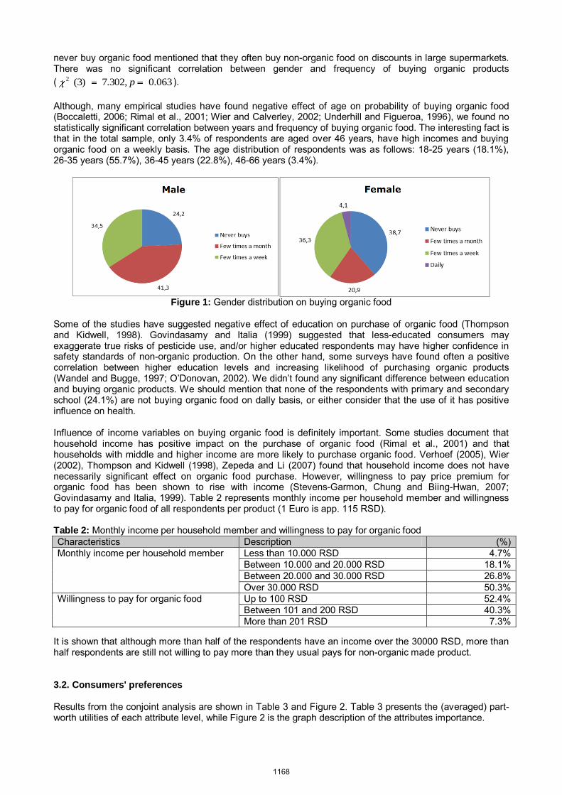
never buy organic food mentioned that they often buy non-organic food on discounts in large supermarkets. There was no significant correlation between gender and frequency of buying organic products ( 2 (3) 7.302, 0.063p ). Although, many empirical studies have found negative effect of age on probability of buying organic food (Boccaletti, 2006; Rimal et al., 2001; Wier and Calverley, 2002; Underhill and Figueroa, 1996), we found no statistically significant correlation between years and frequency of buying organic food. The interesting fact is that in the total sample, only 3.4% of respondents are aged over 46 years, have high incomes and buying organic food on a weekly basis. The age distribution of respondents was as follows: 18-25 years (18.1%), 26-35 years (55.7%), 36-45 years (22.8%), 46-66 years (3.4%).

Figure 1: Gender distribution on buying organic food

Some of the studies have suggested negative effect of education on purchase of organic food (Thompson and Kidwell, 1998). Govindasamy and Italia (1999) suggested that less-educated consumers may exaggerate true risks of pesticide use, and/or higher educated respondents may have higher confidence in safety standards of non-organic production. On the other hand, some surveys have found often a positive correlation between higher education levels and increasing likelihood of purchasing organic products (Wandel and Bugge, 1997; O’Donovan, 2002). We didn’t found any significant difference between education and buying organic products. We should mention that none of the respondents with primary and secondary school (24.1%) are not buying organic food on dally basis, or either consider that the use of it has positive influence on health. Influence of income variables on buying organic food is definitely important. Some studies document that household income has positive impact on the purchase of organic food (Rimal et al., 2001) and that households with middle and higher income are more likely to purchase organic food. Verhoef (2005), Wier (2002), Thompson and Kidwell (1998), Zepeda and Li (2007) found that household income does not have necessarily significant effect on organic food purchase. However, willingness to pay price premium for organic food has been shown to rise with income (Stevens-Garmon, Chung and Biing-Hwan, 2007; Govindasamy and Italia, 1999). Table 2 represents monthly income per household member and willingness to pay for organic food of all respondents per product (1 Euro is app. 115 RSD). Table 2: Monthly income per household member and willingness to pay for organic food

Characteristics Description (%) Monthly income per household member Less than 10.000 RSD 4.7%

Between 10.000 and 20.000 RSD 18.1% Between 20.000 and 30.000 RSD 26.8% Over 30.000 RSD 50.3%

Willingness to pay for organic food Up to 100 RSD 52.4% Between 101 and 200 RSD 40.3% More than 201 RSD 7.3%

It is shown that although more than half of the respondents have an income over the 30000 RSD, more than half respondents are still not willing to pay more than they usual pays for non-organic made product. 3.2. Consumers' preferences Results from the conjoint analysis are shown in Table 3 and Figure 2. Table 3 presents the (averaged) part-worth utilities of each attribute level, while Figure 2 is the graph description of the attributes importance.

1168

Table 3: Averaged results Attribute Attribute level Part-worth utilities Std. dev.

Production method Non-organic production -0.300 0.121 Non-certified organic production -0.340 0.097 Certified organic production 0.640 0.121

Product origin Serbia 0.220 0.072 Abroad -0.220 0.072

Price [RSD]

50 RSD/kg (0.5 €/kg) -0.587 0.072 100 RSD/kg (1 €/kg) -1.174 0.145 150 RSD/kg (1.5 €/kg) -1.761 0.217 200 RSD/kg (2 €/kg) -2.348 0.290 250 RSD/kg (2.5 €/kg) -2.936 0.362

Constant 4.311 Price Coefficient (β) -0.012

Correlations between observed and estimated preferences Pearson's R 0.949 Significance = 0.000

Kendall's tau 0.882 Significance = 0.000

The internal and predictive validity of the rating model was estimated by Pearson and Kendall’s tau statistics. A high value of the Pearson coefficient, 0.949, confirms the high level of significance of the obtained results. Similarly, a high value of the Kendall’s tau statistic, 0.882, indicates the strong correlation between the observed preferences and those estimated by the model. The β coefficient is related to the price attribute, because it is the only attribute defined as linear in SPSS software. This coefficient is always negative for the price and it represents the sensitivity of respondents' preferences on changes in price of products. Higher absolute value of the coefficient and steeper linear function means that respondents are more sensitive to changes in price, meaning that small increase in price leads to a sharp drop of preferences.

35.39%

14.36%

50.25%

0.00%

10.00%

20.00%

30.00%

40.00%

50.00%

60.00%

Production method Production origin Price

Figure 2: Relative importance of attributes

As Figure 2 shows, the most important attribute is Price, with an relative importance value of 50.25%. Than follows the attribute Production method (relative importance = 35.39%). Product origin (14.36%) is the least important attribute. Characteristics that describe „the most desirable carrot“ are: Certified organic production, made in Serbia, at the price of 50 RSD/kg (0.5 €/kg).

3.3. Post hoc segmentation

A more detailed analysis of individual utilities revealed wide heterogeneity in preferences. Therefore, a cluster analysis was performed to classify respondents into more homogeneous preference groups. The part-worths are used as input for cluster analysis.

The K-means cluster procedure in SPSS 16.0 was used to perform the segmentation. A 2-cluster solution was chosen due to the size of the segments and statistical significance. An analysis of variance revealed that

1169

the segments in the 2-cluster solution differed significantly from each other, with respect to their part-worths generated by the conjoint analysis (see Table 4 and Figure 3). Table 4: Segment-level part-worth utilities

Attribute Attribute level Segment 1 (34.9%) Segment 2 (65.1%) Part-worth utilities Part-worth utilities

Production method

Non-organic production 0.11 -0.52 Non-certified organic production -0.24 -0.39 Certified organic production 0.13 0.92

Product origin Serbia 0.51 0.06 Abroad -0.51 -0.06

Price [RSD]

50 RSD/kg (0.5 €/kg) -0.448 -0.661 100 RSD/kg (1 €/kg) -0.896 -1.323 150 RSD/kg (1.5 €/kg) -1.344 -1.984 200 RSD/kg (2 €/kg) -1.793 -2.646 250 RSD/kg (2.5 €/kg) -2.241 -3.307

11.57%

32.10%

56.34%

34.12%

3.02%

62.86%

0.00%

10.00%

20.00%

30.00%

40.00%

50.00%

60.00%

70.00%

Productionmethod

Production origin Price

Segment 1 Segment 2

25

Figure 3: Segment-level attributes importance

As it is shown in Figure 3, price of the product is the most important attribute in both segments. Given the current situation and weak purchasing abilities in Serbia, as a result of the global economic crisis, it is expected that the price was determining factor when buying organically produced food (specifically carrots). The first segment covers more than a third of the total number of respondents (34.9%). Respondents in this segment are equally important whether something is produced in non-organic or organic certified way, but this is an attribute that is not so important to them, and for that reason, they don`t find the difference between levels. On the other hand, the second segment was significantly larger (65.1%) and consists of respondents who are big supporters of organic food, which has an official certificate. The respondents from segment 2 find the origin as a lowest important attribute, and there is almost no difference whether food is produced in Serbia or abroad. Product origin almost does not affect the preferences of the members of this segment.

4. CONCLUSION

In a process of purchasing organic food, there is a significant number of factors that influence the final customer decision on purchasing organic products. Decision for purchasing is something that is evolving and maturing in customers mind and sometimes even the product itself is not main motive for decision. The aim of this paper was to show that the production of organic food is a great development opportunity of Serbia in the future, so we explored preferences of consumers in Serbia towards the carrot. For this purpose we used conjoint analysis. The most important attribute of carrot is Price followed by attributes Production method and Product origin, which is to be expected given the current purchasing power in Serbia. It is evident that on customers’ behaviour socioeconomic and demographic variables has some influence. Faced with the dilemma of choice between organic and non-organic, consumers have different reactions. Female consumers are inherently more rational than male. Demographic results show that still a small number of respondents buy organic food. These results suggest that there is a small consumer base for

1170

organic food and market potential is weak. We also came to conclusion that population is not familiar enough with the methods of production and the benefits of organic food.

In Serbia, above all, it is necessary to provide constant education on organic farming. From organic farming, everyone would have benefits. Our organic food can be exported to EU countries where it has already been observed that people who regularly use organic products improved their life quality. Organic farming essentially aims to save the environment along with high quality production, which is another important aspect. Successful economic development, preserved nature and healthier people - the only question is whether we will take advantage of these opportunities? But above all, the knowledge that we are eating really healthy food and still not destroying the land that feeds us, is in ourselves.

REFERENCES

Aizaki, H. (2010). Application of multi-attributes stated preference methods and conjoint analysis in agricultural economics in Japan: from the latter half of the 1990s to 2005, Technical Report of the National Institute for Rural Engineering.

Boccaletti, S. (2006). Household Behaviour and environmental policy: Review of empirical Studies on Environmental policy: Empirical Evidence and Policy Issues, OECD Environment Directorate 15-16.

Champ, P., Boyle, K., and Brown, T. (2003). A primer on nonmarket valuation. Dordrecht, The Netherlands. Evans, C. B. (2008), Consumer Preferences For Watermelons: A Conjoint Analysis, A Thesis Submitted to

the Graduate Faculty of Auburn University. Govindasamy, R., & Italia, J. (1999). Predicting Willingness-To-Pay A Premium For Organically Grown Fresh

Produce, Journal of Food Distribution Research, Food Distribution Research Society 30(2). Green, P., and V. Srinivasan. (1978). Conjoint analysis in consumer research: issues and outlook. Journal of

Consumer Research. 5: 103-123. Hair, J., Anderson, R., Тatham, W., and Black, W. (1999). Analisis Multivariante. Quinta Edición. Prentice-

hall. Iberia, Madrid, Espana. Lancaster, K. (1971). Consumer demand: A new Approach. Columbia University Press, New York, United

States. 177 pp. Loureiro, M. L., McCluskey, J. J., & Mittelhammer, R. C. (2001). Assessing Consumer Preferences for

Organic, Eco-labelled, and Regular Apples, Journal of Agricultural and Resource Economics 26(2). Lusk, J., & Hudson, D. (2004). Willingness-to-pay estimates and their relevance to agribusiness decision

making. Review of Agricultural Economics, 26: 152–169. Manalo, A. B. (1990). Assessing The Importance Of Apple Attributes: An Agricultural Application Of Conjoint

Analysis. Northeastern Journal of Agricultural and Resource Economics, 19(2). O’Donovan,P., & McCarthy,M. (2002). Irish consumer preference for organic meat, British Food Journal, 104. Rimal, A., Fletcher, S. M., McWatters, K. H., Misra, S. K., & Deodhar, S. (2001). Perception of food safety

and changes in food consumption habits: a consumer analysis, International Journal of Consumer Studies 25(1).

Stevens-Garmon, J., Chung L. H., & Biing-Hwan, L. (2007). Organic Demand: A Profile of Consumers in the Fresh Produce Market, Choices, Agricultural and Applied Economics Association 22(2).

Sydorovych, O., & Wossink, A. (2008). An Application of Conjoint Analysis in Agricultural Sustainability Assessment, International Congress, European Association of Agricultural Economists.

Thompson, G. D., & Kidwell, J. (1998). Explaining the Choice of Organic Produce: Cosmetic Defects, Prices, and Consumer Preferences, American Journal of Agricultural Economics 80(2).

Underhill, S. E., & Figueroa, E. E. (1996). Consumer Preferences For Non-Conventionally Grown Produce, Journal of Food Distribution Research, Food Distribution Research Society, 27(2).

Verhoef, P.C. (2005). Explaining purchases of organic meat by Dutch consumers, European Review of Agricultural Economics, 32(2).

Walisinghe, R., & Gunaratne, P. (2008). Consumer Preferences for Quality Attributes of Rice: A Conjoint Analysis, Sri Lankan Journal of Agricultural Economics 10(11).

Wandel, M., & Bugge, A. (1997). Environmental concern in consumer evaluation of food quality, Food Quality and Preference, 8(1).

Wang, Q., & Sun, J. (2003). Consumer preference and demand for organic food: Evidence from a Vermont survey. American Agricultural Economics Association Annual Meeting in Montreal, Canada.

Wier, M., & Calverley, C. (2002). Market potential for organic foods in Europe, British Food Journal, 104(1). Zepeda, L., & Li, J. (2007). Characteristics of Organic Food Shoppers, Journal of Agricultural and Applied

Economics, Southern Agricultural Economics Association, 39(1).

1171

MATHEMATICAL MODEL OF OPTIMAL ECONOMIC PLAN FOOD FOR LUNCH MEMBERS OF SERBIAN ARMY

Branko Tesanovic,1 Sasa Jovic,2Jelena Tesanovic3

1 Military Academy, University of Defence, brate@verat.net 2 Military institution „Morovic”, sudimnja@gmail.com

3 Municipality „Ieastern Saraevo“, Serbo Republic Abstract: In order to improve the economy of nutrition in the army of Serbia (hereinafter referred to as AS) there is a need to organize food surcharge during the working hours of professional members AS. Insufficient employment existing workforce and high overheads, the barriers are to reduce the amount of the total cost of food in AS. By using the software package LP Solve with multi-criteria analysis, based on nutritional value and biological food products (hereafter FP), their prices and food needs of professional members of the Army, leads to the development of a mathematical model of economic optimal eating plan for lunch. Keywords: Multi-criteria analysis, LP Solve, energy value of foods, nutritional value of food, nutrition in the

workplace, economically optimal nutrition, eating lunch.

1. INTRODUCTION

Tests for food in AS1 by many authors, such as B. Tesanovic and others point to the fact that nutrition can examine the qualitative and quantitative aspects. The qualitative aspect consists in the application of highly effective nutrition programs that provide health-safe and balanced diet of consumers. In this paper, the qualitative aspect of nutrition is analyzed primarily from the perspective of developing economically optimal eating plan of AS for lunch, as lunch is the meal by which in the course of the day brings the highest volume of energy and nutritive substances in the body.

2. NUTRITION IN THE WORKPLACE PAY IN SERBIAN ARMY

The consequences of malnutrition are very common throughout the world. Eating habits are conditioned by the greater number of factors: the need to enjoy food, real needs, scientific knowledge, and other economic factors. Under the eating habits of an individual involves the selection and preparation, the amount, time and manner of consumption of FP for a longer period (Pelva, 2010). The main normative act that regulates food in AS the Ordinance on general and logistical needs of the Department of Defense (hereafter DoD) and AS (hereinafter referred to as the Ordinance). Ordinance regulating norms belonging to FP. Prescribed norms should provide nutrition based on scientific principles and align with the physical needs of AS and specific military requirements. In order to implement the provisions of the Regulations are made diet plans that are based on the statutory structure of FP , norms belonging and recipes for cooking in AS. Abolition of compulsory military service (Jovic , 2013) the number of persons who are entitled to free meals, reduced to 4.000 persons. In order to develop the economy of nutrition, and increase the level of installed capacity employment military Restaurant (hereafter MR) there is a need to organize meals for a fee, which must meet the energy and nutritional needs in food. Activities carried out by members of the AS can be classified as medium hard physical work, and to satisfy their daily energy needs should be provided daily meals (hereinafter referred to as d/m) feed containing about 14.700 KJ (Jokic, 1998). From that lunch should provide about 40% of the energy value of d/m food. According to the recommendations of the World Health Organization's share of nutrients in the total energy value of d/m is: for protein - 10 to 15 % ; the fat content - 15 to 30 % of carbohydrates, and - 55 to 75 %.

1 According to the Regulations on general logistics needs of DoD and "nutrition personnel the task of the general logistic

function, which is achieved on the basis of scientific knowledge, technological capabilities, experiences, habits and traditions in the diet of the population, in line with the psychological and physical stresses and demands concerted command and management as prescribed, regular health and proper way provides high quality and totally satisfying energy-biological needs of the professional members of AS. Nutrition in AS is planned, programmed and organized by the eating plan in AS.“

1172

Interest in nutrition surcharge in AS so far is small. Insufficient employment installed capacity of MR, the existing workforce and high overheads, the barriers are to reduce the amount of the total cost of providing food services at the workplace, thereby preventing an increase in the number of people who would be interested for this type of diet.

In order to provide all members of the MS one meal during the working time necessary to plan adequate funds to pay for it in the form of refunds from the approved budget allocations for food (Jovic, 2010). In order to achieve quality food, which is the economic aspect of production is acceptable, and which also meets the nutritional standards of quality, it is necessary to produce food that has an acceptable level of costs, and that is an acceptable range by members of the AS. It is necessary to create a proposal for a diet plan for lunch, which will ensure the proper and balanced diet for this meal, with the use of nutritional and economic criteria. This diet plan ought to include standardized menus , application menu cycle, plan expenditure of FP and an explanation of its use, but which are related to food during working hours and that includes just one meal instead of all day d/m food. Normative consumption of FP and food preparation should be adapted to the needs of the organism, since it would be realized only one meal, and that the remaining two lunch time staff consumed outside the workplace. The next section of the paper presents a general and then a special mathematical model diet surcharge in the Army, based on the study of optimal model diet plan for lunch.

3. DRAFT ANNUAL PLAN OF SERBIAN FOOD IN THE ARMY FOR LUNCH - GENERALMATHEMATICAL MODEL

The main objective of the research in this paper is the Definition of diet plans for lunch, to establish a cost-effective nutrition surcharge ie. build a model that is optimal from an economic point of view, and that meets the predetermined energy and biological constraints and needs of the AS in the diet. Problem diet surcharge aims to making a diet plan for lunch, while minimizing the cost of food and meeting pre-defined energy and biological constraints and needs of the AS. For solving this problem affected by many factors, such as price FP, meals and menus, Percentage of different types of FP in nutrition and others.

Taking into account the limiting factors can be obtained as a result of Plan meals for lunch, which is the optimal solution from an economic point of view. The daily menus using the multi-criteria analysis, based on the analysis of energy and biological value of FP, FP prices and food needs of AS, leads to the development of combination dishes that. Daily menu for lunch. Each set contains: name of FP, quantity, energy value and amounts of nutrients. Determining the number of application of certain foods that are part of the handle defines a cycle of application meals. When preparing meals Cycle application, you need to meet several criteria: variety of food; appreciation of the seasonal character of FP; achieve the planned average energy-biological value lunch and planned expenditure FP. Price changes FP from the economic point of view is a significant limitation in the development cycle, the application meals.

In developing the model diet plan for lunch, as a starting point for the implementation recipes for making lunch, we used data from the eating plan in AS. In this diet plan defines the 133 recipes that can become part of lunch. By using the software package LP Solve, set the basic - a general mathematical model for the development of the Plan daily menus, with appropriate mathematical assumptions and limitations. Of the initial parameters for the development of a model diet plan are: FP, meal and menu. Based on these recipes for making lunch in the eating plan in AS and quantitative participation of FP, which are included in the prices of certain food dishes.

Mathematical assumptions are: a) the linearity of the objective function, b) linearity constraints, c) a finite number of constraints and d) additivity constraints and objective functions.

Based on these assumptions math was done setting the general mathematical model of cost-effective nutrition surcharge ie. build a model that will be the economic aspect of optimal, and that will meet predetermined energy and biological constraints and needs of the VS in the diet:

The criterion of optimality of linear objective function with respect to the restrictions:

(1)

where: F (objective function), C (the coefficients of the variables in the objective function) and Xi (variable) .

1173

Restrictions: a11Х1 + a12Х2 +...+ a1nХn ≤b1 a21Х1 + a22Х2 +...+ a2nХn ≤b2 ........................................... am1Х1 + am2Х2 +...+ amnХn ≤bm

where: aij (the coefficients of the variables in constraints), C (coefficient restrictions) and Xi (variable). On the basis of a general plan daily menus are made suggestions of specific models of the Plan daily menus for lunch. 4. PROPOSAL OF THE YEARLY DIET PLANS IN THE SERBIAN ARMY FOR LUNCH In order to develop a specific model plan daily menus for lunch, it is necessary for a total of 83 main dishes, 11 types of soup (broth), 12 salads, 18 types of cakes and 9 species of fruit eating plan approved in AS find the frequency of each of them on an annual basis for 252 working days, taking into account the biological and energy constraints, to achieve the minimum total cost of the food. It is necessary to take into account that the number of cakes and fruit number of alternative variables, ie. that their sum total is 252 for lunch as part of the diet plan participates cake or fruit. On the basis of standardized meals for lunch and preparation of statistical data on the average energy value and composition of nutrients shown to diet plans in the AS, and the price of individual FP forming part of the meal was made the budget share of proteins, fats and carbohydrates in each of dishes, as well as the price of food, which are used in the preparation of the handles. The above data are shown in Tables 1 – 5. Table 1. The percentage share of protein, fat and carbohydrate composition of the soup

Variable Kind of soup The energy value (Cal)

% Of the amount of food Price in dinars Proteins Fat Carbohydrates Х96 Soup of the concentrate with stars 123,10 12,3 2,8 84,9 2,10 Х97 Beef soup with stars 177,32 9,7 24,3 66,0 1,77 Х98 Chicken soup with stars 318,95 23,7 39,6 36,7 6,39 Х99 Chicken soup 662,96 15,5 49,0 35,5 11,14 Х100 Beef soup 743,29 13,9 54,4 31,7 20,44 Х101 Cream of mushroom soup 567,17 10,7 44,3 45,0 13,46 Х102 Split pea soup 634,95 17,4 33,0 49,6 4,34 Х103 Tomato soup with rice 464,68 5,9 44,4 49,7 6,22 Х104 Potato soup 463,23 6,2 43,4 50,4 5,16 Х105 Vegetable soup 464,47 7,3 43,7 49,0 9,08 Х106 Fish soup 642,18 22,0 43,6 34,4 15,18

Average 478,39 13,15 38,41 48,45 8,66

Source: Plan meals in AS and authors' calculations Table 2. The percentage share of protein, fat and carbohydrate composition of the main dishes

Variable Types of main dishes The energy value (Cal)

% Of the amount of food Price in dinars Proteins Fat Carbohydrates

Х1 Bean soup with smoked pork 1050,02 16,9 21,5 61,6 62,30 Х2 Dry bean soup with bacon 1361,05 13,1 39,4 47,5 58,06 Х3 Military beans 1144,85 18,3 22,8 58,9 81,02 Х4 Roast pork and beans 1326,90 16,0 30,2 53,8 68,77 Х5 Fried fish and beans 1275,62 23,6 18,9 57,5 81,94 Х6 Steak, braised green beans and potatoes 1257,44 15,0 32,9 52,1 126,67 Х7 Steak, mashed spinach and rice 1234,73 15,3 33,9 50,8 113,51 Х8 Leskovac shaker and salted potatoes 1063,00 13,7 24,8 61,5 88,69 Х9 Cooked beef in tomatoes sauce, potatoes and cauliflower 1163,74 13,2 33,3 53,5 91,40 Х10 Cooked beef in tomatoes sauce, roasted potatoes and

braised peas 1026,79 16,2 31,6 52,2 104,25

Х11 Beef, cooked fresh pasta and braised cabbage 931,90 14,8 38,6 46,6 81,17 Х12 Beef and potatoes 1113,98 14,3 28,6 57,1 84,00 Х13 Sirloin in natural jus and a fine stew 1153,01 15,3 30,5 54,2 124,06 Х14 Beef sirloin, baked potato and braised cabbage 1040,26 14,2 41,2 44,6 85,92 Х15 Braised beef steak, braised carrots and roasted potatoes 982,17 13,0 35,7 51,3 76,18 Х16 Braised beef steak, braised green beans and braised rice 1118,82 13,4 31,9 54,7 106,55 Х17 Beef stew, cooked pasta and braised cabbage 899,45 14,0 35,7 50,3 95,87 Х18 Beef stew and mashed potatoes 1081,40 13,6 25,9 60,5 101,21 Х19 Meat loaf, mashed potatoes with spinach and roasted

potatoes 944,09 15,7 29,6 54,7 91,50

Х20 Meat loaf and rice 1104,82 13,9 19,8 66,3 66,35 Х21 Meat loaf, braised peas and mashed potatoes 1127,65 15,3 22,8 61,9 94,30 Х22 Saute beef "stroganoff" and potatoes 1112,20 13,7 29,2 57,1 94,56

1174

Х23 Parisian steak and baked potato 884,77 14,3 36,9 48,8 73,51 Х24 Parisian steak, braised green beans and salted potatoes 1078,96 13,7 32,2 54,1 108,53 Х25 Wiener schnitzel, braised peas and mashed potatoes 1199,17 14,9 28,6 56,5 85,46 Х26 Wiener schnitzel, braised cabbage and roasted sweet

potatoes 990,07 13,8 38,8 47,4 76,11

Х27 Kebabs and roasted potatoes 859,34 14,1 38,7 47,2 75,37 Х28 Burger, braised peas and roasted potatoes 1027,74 15,2 36,3 48,5 104,45 Х29 Natur steak and fine stew 1197,72 12,6 36,3 51,1 76,24 Х30 Natur steak, braised cabbage and sweet braised rice 1163,25 10,5 41,4 48,1 54,84 Х31 Roast pork, cabbage and mashed potatoes 1247,83 11,2 42,4 46,4 63,74 Х32 Pork roast, braised peas and potatoes 1026,57 12,8 39,6 47,6 81,85 Х33 Pork roast, braised cabbage and roasted potatoes 979,30 11,1 45,7 43,2 60,80 Х34 Pork chop in garlic and roasted potatoes 925,46 11,7 44,3 44,0 60,60 Х35 Skewered and roasted potatoes 907,92 11,2 44,1 44,7 56,62 Х36 Chop (grilled) stewed green beans and baked potato 1066,75 11,1 47,4 41,5 98,00 Х37 Chicken (grilled), fried cauliflower and tartar soup 939,27 19,0 32,8 48,2 68,41 Х38 Chicken (grilled), pureed spinach and mashed potatoes 960,43 20,7 17,9 61,4 83,54 Х39 Chicken (grilled), stewed peas and potatoes 980,16 20,7 15,6 63,7 89,34 Х40 Sauteed chicken, braised rice and sweet cabbage 1115,43 17,5 31,5 51,0 67,98 Х41 Fried chicken, braised carrots and mashed potatoes 1086,17 16,9 21,6 61,5 60,63 Х42 Fried chicken, braised green beans and potatoes 903,71 18,4 27,9 53,7 121,10 Х43 Roast chicken, cabbage and mashed potatoes 1124,36 18,9 29,6 51,5 64,99 Х44 Roast chicken, braised peas and roasted potatoes 921,61 22,2 24,8 53,0 80,10 Х45 Stew and polenta 1097,46 20,3 27,2 52,5 62,10 Х46 Grilled fish and asparagus in coastal way 979,60 19,0 27,9 53,1 57,74 Х47 Baked fish on onions and salted potatoes 1039,71 18,5 21,7 59,8 58,88 Х48 Baked fish (grilled) and Swiss chard fashioned 887,77 21,9 19,5 58,6 149,22 Х49 Baked fish (grilled) and salted potatoes 936,80 21,4 13,4 65,2 117,52 Х50 Fried fish and potato salad 844,58 23,6 28,3 48,1 67,06 Х51 Fried fish, mashed spinach and roasted potatoes 985,23 21,0 32,2 46,8 92,76 Х52 Fried fish and fried potatoes 871,82 20,7 33,0 46,3 67,06 Х53 Roasted lamb, braised peas and roasted potatoes 986,93 15,6 34,9 49,5 155,17 Х54 Sheep roast, braised peas and roasted potatoes 949,75 15,5 33,1 51,4 141,37 Х55 Roast turkey and baked potatoes 853,40 17,4 34,6 48,0 107,82 Х56 Roast turkey and cabbage 945,99 18,3 34,5 47,2 110,80 Х57 Moussaka cauliflower 878,65 16,3 31,1 52,6 91,18 Х58 Sauerkraut with smoked pork 886,75 14,4 34,5 51,1 64,36 Х59 Lamb caps 911,17 15,4 34,3 50,3 135,71 Х60 Moussaka of eggplant blue 1101,88 14,8 36,8 48,4 128,30 Х61 Zucchini moussaka 964,16 16,2 32,0 51,8 80,61 Х62 Beef in vegetables 1018,07 14,9 29,1 56,0 82,20 Х63 Hunting potatoes with meat 1055,21 13,5 26,2 60,3 73,30 Х64 Moussaka potato 837,20 16,4 34,1 49,5 66,91 Х65 Sarma with sauerkraut 1330,74 12,5 36,4 51,1 91,44 Х66 Stuffed peppers 1100,60 13,5 27,0 59,5 83,94 Х67 Stuffed zucchini 1150,13 13,1 29,9 57,0 85,34 Х68 Greek meatballs 958,11 16,3 24,6 59,1 72,08 Х69 Potato stew with beef meat 1072,06 13,1 27,4 59,5 71,78 Х70 Soy steak with sautéed mushrooms and potatoes 937,10 17,7 26,5 55,8 62,90 Х71 Soy steak and beans 1345,67 19,3 20,7 60,0 45,00 Х72 Beans military (fasting) 1240,06 19,3 21,0 59,7 38,04 Х73 Pasta in tomato sauce with tuna 966,03 29,9 27,0 43,1 99,82 Х74 Risotto with fish 1107,38 21,5 19,9 58,6 77,53 Х75 Risotto with mushrooms 912,80 12,7 15,0 72,3 73,90 Х76 Peppers stuffed with beans 1035,25 15,3 20,6 64,1 46,54 Х77 Peppers stuffed (fasting) 980,18 13,4 30,1 56,5 74,03 Х78 Sarma with sauerkraut (fasting) 1077,75 13,8 32,4 53,8 34,83 Х79 Soy steak, cabbage (fasting) and baked potato 1139,08 15,1 37,6 47,3 40,35 Х80 Fried mushrooms and fried potatoes 658,59 15,2 19,3 65,5 99,44 Х81 Braised mushrooms and braised rice 1027,25 12,2 18,2 69,6 96,53 Х82 Soy steak, stewed peas and potatoes (in water) 1239,34 17,1 23,0 59,9 58,46 Х83 Stew of soybean and potato (water) 1017,34 16,1 22,5 61,4 28,25

Source: Plan meals in AS and authors' calculations

Table 3. The percentage share of protein, fat and carbohydrate composition of the salad Variable Types of salad The energy

value (Cal) % Of the amount of food Price in dinars Proteins Fat Carbohydrates

Х84 Green salad 174,47 9,1 69,1 21,8 18,58 Х85 Spring onions 43,93 14,9 4,3 80,8 20,00 Х86 Fresh cucumbers 166,86 10,1 50,0 39,9 6,10 Х87 Tarator salad 342,99 21,8 50,5 27,7 14,57 Х88 Fresh tomatoes 324,01 11,9 43,1 45,0 49,00 Х89 Fresh cabbage 295,44 6,7 67,2 26,1 5,00 Х90 Roasted peppers 385,95 8,6 53,6 37,8 11,80

1175

Х91 Mixed fresh vegetables 371,35 8,6 56,8 34,6 30,30 Х92 Pickles 68,20 26,4 17,1 56,5 34,50 Х93 Salad with sour peppers 155,62 19,8 7,5 72,7 31,50 Х94 Pickled cabbage 323,21 11,2 65,8 23,0 3,51 Х95 Beetroot (pasteurized) 232,01 9,9 2,5 87,6 22,50

Average 240,34 13,25 40,63 46,13 20,61

Source: Plan meals in AS and authors' calculations Table 4. The percentage share of protein, fat and carbohydrate composition of the pie

Variable Types of pie The energy value (Cal)

% Of the amount of food Price in dinars Proteins Fat Carbohydrates Х107 Pudding 244,20 9,9 18,3 71,8 16,71 Х108 Cake with eggs 363,50 9,1 17,7 73,2 13,76 Х109 Rice cakes 298,80 14,1 18,9 67,0 15,30 Х110 Cake frozen 369,25 10,0 10,0 80,0 120,01 Х111 Donuts frozen 369,25 10,0 10,0 80,0 120,85 Х112 Cherry pie frozen 384,63 5,1 35,2 59,7 120,00 Х113 Apple pie frozen 371,48 5,0 38,2 56,8 170,00 Х114 Cream pie with biscuit 195,18 9,4 20,9 69,7 35,38 Х115 Turkish pole 413,35 4,1 25,2 70,7 17,74 Х116 Princes donuts 305,85 10,2 46,9 42,9 13,04 Х117 Ice asks 377,17 4,8 49,6 45,6 7,20 Х118 Fruit cake, industrial 369,25 10,0 10,0 80,0 386,00 Х119 Chocolate rolls, industrial 369,25 10,0 10,0 80,0 386,00 Х120 Chocolate cake 378,06 4,3 52,0 43,7 18,61 Х121 Fruit roll 320,21 4,6 47,7 47,7 18,44 Х122 Pie pumpkin 545,28 8,8 35,0 56,2 10,20 Х123 Ice cream, industrial 158,30 7,8 35,2 57,0 22,00 Х124 Fruit salad 228,03 2,8 4,4 92,8 23,95

Average 336,72 7,78 26,96 65,27 84,18

Source: Plan meals in AS and authors' calculations Table 5. The percentage share of protein, fat and carbohydrate composition of the fruit

Variable Types of fruit The energy value (Cal)

% Of the amount of food Price in dinars Proteins Fat Carbohydrates Х125 Pears 97,39 3,5 5,9 90,6 24,00 Х126 Grapes 159,47 4,1 5,3 90,6 32,50 Х127 Watermelon 56,66 8,1 6,1 85,8 21,00 Х128 Orange 65,87 6,7 2,5 90,8 25,00 Х129 Bananas 142,69 4,5 3,7 91,8 22,00 Х130 Tangerine 136,53 44,4 0,0 55,6 27,50 Х131 Apple 109,46 2,3 5,3 92,4 20,00 Х132 Cherry 140,92 6,6 6,0 87,4 25,00 Х133 Peach 103,30 6,1 3,9 90,0 19,50

Average 112,48 9,59 4,30 86,11 24,06

Source: Plan meals in AS and authors' calculations Assuming that the total number of main dishes, salads, soups, cakes and fruit per annum equal to the number of working days, set limits are shown in Table 6.

Table 6. Frequency limits on the types of food for lunch Type of food Limitations Entrees Х1+Х2+Х3+....+Х81+Х82+Х83= 252 Salads Х84+Х85+Х86+Х87+Х88+Х89+Х90+Х91+Х92+Х93+Х94+Х95=252 Soup-stew Х96+Х97+Х98+Х99+Х100+Х101+Х102+Х103+Х104+Х105+Х106=252 Cakes and Fruit Х107+Х108+Х109+...+Х131+Х132+Х133=252

Source: Authors' calculations Due to the high cost of input points, and in relation to the need to meet the biological and energetic constraints placed additional restrictions on the minimum number of occurrences of certain cakes and dishes, presented in Table 7 and: Table 7. The default limits the minimum number of occurrences of dishes

Х107+Х108+Х109+Х110+Х111+Х112+Х113+Х114+Х115+Х116+Х117+Х118+Х119+Х120+Х121+Х122+Х123+Х124>=26 Х22+Х23>=1 Х24+Х25>=1 Х26+Х27>=1 Х48+Х64+Х65+Х73+Х74>=1

Source: Authors' calculations Taking into account that the composition of the meal for lunch has a larger number of components, ie. soup - soup, main course, salad and dessert or fruit, set the share of each of these dishes in the composition of the

1176

handle on the quantitative amount of their shares, based on which further set linear constraints in relation to the biological requirements, as well as in relation to the demand:

а) For proteins: 6,2Х1+4,8Х2+6,7Х3+5,9Х4+8,7Х5+5,5Х6+5,6Х7+5Х8+4,8Х9+5,9Х10+5,4Х11+5,3Х12+5,6Х13+5,2Х14+4,8Х15+4,9Х16+5,1Х17+5Х18+5,8Х19+5,1Х20+5,6Х21+5Х22+5,3Х23+5Х24+5,5Х25+5,1Х26+5,2Х27+5,6Х28+4,6Х29+3,8Х30+4,1Х31+4,7Х32+4,1Х33+4,3Х34+4,1Х35+4,1Х36+7Х37+7,6Х38+7,6Х39+6,4Х40+6,2Х41+6,8Х42+6,9Х43+8,2Х44+7,5Х45+7Х46+6,8Х47+8,1Х48+7,9Х49+8,7Х50+7,7Х51+7,6Х52+5,8Х53+5,8Х54+6,4Х55+6,8Х56+6Х57+5,3Х58+5,7Х59+5,4Х60+6Х61+5,5Х62+5Х63+6Х64+4,6Х65+5Х66+4,8Х67+6Х68+4,8Х69+6,5Х70+7,1Х71+7,1Х72+11Х73+7,9Х74+4,7Х75+5,6Х76+4,9Х77+5,1Х78+5,5Х79+5,5Х80+4,5Х81+6,3Х82+5,9Х83+1Х84+1,6Х85+1,1Х86+2,4Х87+1,3Х88+0,7Х89+0,9Х9

0+0,9Х91+2,9Х92+2,1Х93+1,2Х94+1Х95+2,7Х96+2,1Х97+5,2Х98+3,4Х99+3Х100+2,3Х101+3,8Х102+1,3Х103+1,3Х104+1,6Х105+4,8Х106+1Х107+1Х108+1,5Х109+1,1Х110+1,1Х111+0,5Х112+0,5Х113+1Х114+0,4Х115+1,1Х116+0,5Х117+1,1Х118+1,1Х119+0,4Х120+0,5Х121+0,9Х122+0,8Х123+0,3Х124+0,6Х125+0,7Х126+1,5Х127+1,2Х128+0,8Х129+8,4Х130+0,4Х131+1,2Х132+1,1Х133>= 2.520;

6,2Х1+4,8Х2+6,7Х3+5,9Х4+8,7Х5+5,5Х6+5,6Х7+5Х8+4,8Х9+5,9Х10+5,4Х11+5,3Х12+5,6Х13+5,2Х14+4,8Х15+4,9Х16+5,1Х17+5Х18+5,8Х19+5,1Х20+5,6Х21+5Х22+5,3Х23+5Х24+5,5Х25+5,1Х26+5,2Х27+5,6Х28+4,6Х29+3,8Х30+4,1Х31+4,7Х32+4,1Х33+4,3Х34+4,1Х35+4,1Х36+7Х37+7,6Х38+7,6Х39+6,4Х40+6,2Х41+6,8Х42+6,9Х43+8,2Х44+7,5Х45+7Х46+6,8Х47+8,1Х48+7,9Х49+8,7Х50+7,7Х51+7,6Х52+5,8Х53+5,8Х54+6,4Х55+6,8Х56+6Х57+5,3Х58+5,7Х59+5,4Х60+6Х61+5,5Х62+5Х63+6Х64+4,6Х65+5Х66+4,8Х67+6Х68+4,8Х69+6,5Х70+7,1Х71+7,1Х72+11Х73+7,9Х74+4,7Х75+5,6Х76+4,9Х77+5,1Х78+5,5Х79+5,5Х80+4,5Х81+6,3Х82+5,9Х83+1Х84+1,6Х85+1,1Х86+2,4Х87+1,3Х88+0,7Х89+0,9Х9

0+0,9Х91+2,9Х92+2,1Х93+1,2Х94+1Х95+2,7Х96+2,1Х97+5,2Х98+3,4Х99+3Х100+2,3Х101+3,8Х102+1,3Х103+1,3Х104+1,6Х105+4,8Х106+1Х107+1Х108+1,5Х109+1,1Х110+1,1Х111+0,5Х112+0,5Х113+1Х114+0,4Х115+1,1Х116+0,5Х117+1,1Х118+1,1Х119+0,4Х120+0,5Х121+0,9Х122+0,8Х123+0,3Х124+0,6Х125+0,7Х126+1,5Х127+1,2Х128+0,8Х129+8,4Х130+0,4Х131+1,2Х132+1,1Х133<= 3.780;

b) For fat:7,9Х1+14,7Х2+8,4Х3+11,1Х4+7Х5+12,1Х6+12,5Х7+9,1Х8+12,3Х9+11,7Х10+14,2Х11+10,5Х12+11,2Х13+15,2Х14+13,2Х15+11,8Х16+13,2Х17+9,5Х18+10,9Х19+7,3Х20+8,4Х21+10,8Х22+13,6Х23+11,9Х24+10,6Х25+14,3Х26+14,3Х27+13,5Х28+13,5Х29+15,3Х30+15,6Х31+14,6Х32+16,9Х33+16,3Х34+16,3Х35+17,5Х36+12,1Х37+6,6Х38+5,7Х39+11,6Х40+8Х41+10,3Х42+10,9Х43+9,1Х44+10Х45+10,3Х46+8Х47+7,2Х48+4,9Х49+10,4Х50+11,9Х51+12,2Х52+12,9Х53+12,2Х54+12,8Х55+12,7Х56+11,5Х57+12,7Х58+12,7Х59+13,6Х60+11,8Х61+10,7Х62+9,7Х63+12,6Х64+13,4Х65+10Х66+11Х67+9,1Х68+10,1Х69+9,8Х70+7,6Х71+7,7Х72+10Х73+7,3Х74+5,5Х75+7,6Х76+11,1Х77+12Х78+13,9Х79+7,13Х80+6,7Х81+8,5Х82+8,3Х83+7,6Х84+0,4Х85+5,5Х86+5,7Х87+4,7Х88+7,3Х89+5,9Х90+6,2Х91+1,8Х92+0,8Х93+7,2Х94+0,2Х95+0,6Х96+5,3Х97+8,7Х98+10,7Х99+11,9Х100+9,7Х101+7,26Х102+9,7Х103+9,5Х104+9,6Х105+9,6Х106+2Х107+1,9Х108+4,1Х109+1,1Х110+1,1Х111+3,8Х112+4,2Х113+4,6Х114+5,4Х115+10,3Х116+5,4Х117+1,1Х118+1,1Х119+5,7Х120+5,2Х121+3,8Х122+3,8Х123+0,4Х124+1,1Х125+1Х126+1,1Х127+0,4Х128+0,7Х129+0Х130+1Х131+1,1Х132+0,7Х133>=3.780;

7,9Х1+14,7Х2+8,4Х3+11,1Х4+7Х5+12,1Х6+12,5Х7+9,1Х8+12,3Х9+11,7Х10+14,2Х11+10,5Х12+11,2Х13+15,2Х14+13,2Х15+11,8Х16+13,2Х17+9,5Х18+10,9Х19+7,3Х20+8,4Х21+10,8Х22+13,6Х23+11,9Х24+10,6Х25+14,3Х26+14,3Х27+13,5Х28+13,5Х29+15,3Х30+15,6Х31+14,6Х32+16,9Х33+16,3Х34+16,3Х35+17,5Х36+12,1Х37+6,6Х38+5,7Х39+11,6Х40+8Х41+10,3Х42+10,9Х43+9,1Х44+10Х45+10,3Х46+8Х47+7,2Х48+4,9Х49+10,4Х50+11,9Х51+12,2Х52+12,9Х53+12,2Х54+12,8Х55+12,7Х56+11,5Х57+12,7Х58+12,7Х59+13,6Х60+11,8Х61+10,7Х62+9,7Х63+12,6Х64+13,4Х65+10Х66+11Х67+9,1Х68+10,1Х69+9,8Х70+7,6Х71+7,7Х72+10Х73+7,3Х74+5,5Х75+7,6Х76+11,1Х77+12Х78+13,9Х79+7,13Х80+6,7Х81+8,5Х82+8,3Х83+7,6Х84+0,4Х85+5,5Х86+5,7Х87+4,7Х88+7,3Х89+5,9Х90+6,2Х91+1,8Х92+0,8Х93+7,2Х94+0,2Х95+0,6Х96+5,3Х97+8,7Х98+10,7Х99+11,9Х100+9,7Х101+7,26Х102+9,7Х103+9,5Х104+9,6Х105+9,6Х106+2Х107+1,9Х108+4,1Х109+1,1Х110+1,1Х111+3,8Х112+4,2Х113+4,6Х114+5,4Х115+10,3Х116+5,4Х117+1,1Х118+1,1Х119+5,7Х120+5,2Х121+3,8Х122+3,8Х123+0,4Х124+1,1Х125+1Х126+1,1Х127+0,4Х128+0,7Х129+0Х130+1Х131+1,1Х132+0,7Х133<= 7.560;

c) For carbohydrates:22,7Х1+15,5Х2+21,8Х3+19,9Х4+21,2Х5+19,2Х6+18,8Х7+22,7Х8+19,8Х9+19,3Х10+17,2Х11+21,1Х12+20Х13+16,5Х14+18,9Х15+20,2Х16+18,6Х17+22,3Х18+20,2Х19+24,5Х20+22,9Х21+21,1Х22+18Х23+20Х24+20,9Х25+17,5Х26+17,4Х27+17,9Х28+18,9Х29+17,7Х30+17,1Х31+17,6Х32+15,9Х33+16,2Х34+16,5Х35+15,3Х36+17,8Х37+22,7Х38+23,5Х39+18,8Х40+22,7Х41+19,8Х42+19Х43+19,6Х44+19,4Х45+19,6Х46+22,1Х47+21,6Х48+24,1Х49+17,7Х50+17,3Х5

1+17,1Х52+18,3Х53+19Х54+17,7Х55+17,4Х56+19,4Х57+18,9Х58+18,6Х59+17,9Х60+19,1Х61+20Х62+22,3Х63+18,3Х64+18,9Х65+22Х66+21Х67+21,8Х68+22Х69+20,6Х70+22,2Х71+22Х72+15,9Х73+21,6Х74+26,7Х75+23,7Х76+20,9Х77+19,9Х78+17,5Х79+24,2Х80+25,7Х81+22,1Х82+22,7Х83+2,4Х84+8,9Х85+4,3Х86+3Х87+4,9Х88+2,8Х89+4,1Х90+3,8Х91+6,2Х92+8Х93+2,5Х94+9,6Х95+18,6Х96+14,5Х97+8Х98+7,8Х99+6,9Х100+9,9Х101+10,9Х102+10,9Х103+11Х104+10,7Х105+7,5Х106+7,9Х107+8Х108+7,3Х109+8,8Х110+8,8Х111+6,5Х112+6,2Х113+7,6Х114+7,7Х115+4,7Х116+5Х11

7+8,8Х118+8,8Х119+4,8Х120+5,2Х121+6,1Х122+6,2Х123+10,2Х124+17,1Х125+17,1Х126+16,3Х127+17,1Х128+17,4Х12

9+10,5Х130+17,4Х131+16,6Х132+17,1Х133>= 13.860;

1177

22,7Х1+15,5Х2+21,8Х3+19,9Х4+21,2Х5+19,2Х6+18,8Х7+22,7Х8+19,8Х9+19,3Х10+17,2Х11+21,1Х12+20Х13+16,5Х14+18,9Х15+20,2Х16+18,6Х17+22,3Х18+20,2Х19+24,5Х20+22,9Х21+21,1Х22+18Х23+20Х24+20,9Х25+17,5Х26+17,4Х27+17,9Х28+18,9Х29+17,7Х30+17,1Х31+17,6Х32+15,9Х33+16,2Х34+16,5Х35+15,3Х36+17,8Х37+22,7Х38+23,5Х39+18,8Х40+22,7Х41+19,8Х42+19Х43+19,6Х44+19,4Х45+19,6Х46+22,1Х47+21,6Х48+24,1Х49+17,7Х50+17,3Х5

1+17,1Х52+18,3Х53+19Х54+17,7Х55+17,4Х56+19,4Х57+18,9Х58+18,6Х59+17,9Х60+19,1Х61+20Х62+22,3Х63+18,3Х64+18,9Х65+22Х66+21Х67+21,8Х68+22Х69+20,6Х70+22,2Х71+22Х72+15,9Х73+21,6Х74+26,7Х75+23,7Х76+20,9Х77+19,9Х78+17,5Х79+24,2Х80+25,7Х81+22,1Х82+22,7Х83+2,4Х84+8,9Х85+4,3Х86+3Х87+4,9Х88+2,8Х89+4,1Х90+3,8Х91+6,2Х92+8Х93+2,5Х94+9,6Х95+18,6Х96+14,5Х97+8Х98+7,8Х99+6,9Х100+9,9Х101+10,9Х102+10,9Х103+11Х104+10,7Х105+7,5Х106+7,9Х107+8Х108+7,3Х109+8,8Х110+8,8Х111+6,5Х112+6,2Х113+7,6Х114+7,7Х115+4,7Х116+5Х11

7+8,8Х118+8,8Х119+4,8Х120+5,2Х121+6,1Х122+6,2Х123+10,2Х124+17,1Х125+17,1Х126+16,3Х127+17,1Х128+17,4Х12

9+10,5Х130+17,4Х131+16,6Х132+17,1Х133<=18.900; г) For the energy value: 1050,02Х1+1361,45Х2+1144,85Х3+1326,9Х4+1275,62Х5+1257,44Х6+1234,73Х7+1063Х8+1163,74Х9+1026,79Х10+931,9Х11+1113,98Х12+1153,01Х13+1040,26Х14+982,17Х15+1118,82Х16+899,45Х17+1081,40Х18+944,09Х19+1104,82Х20+1127,65Х21+1112,2Х22+884,77Х23+1078,96Х24+1199,17Х25+990,07Х26+859,34Х27+1027,74Х28+1197,72Х29+1163,25Х30+1247,83Х31+1026,57Х32+979,3Х33+925,46Х34+907,92Х35+1066,75Х36+939,27Х37+960,43Х38+980,16Х39+1115,43Х40+1086,17Х41+903,71Х42+1124,36Х43+921,61Х44+1097,46Х45+979,6Х46+1039,71Х47+887,77Х48+936,80Х49+844,58Х50+985,23Х51+871,82Х52+986,93Х53+949,75Х54+853,4Х55+945,99Х56+878,65Х57+886,75Х58+911,17Х59+1101,88Х60+964,16Х61+1018,07Х62+1055,21Х63+837,20Х64+1330,74Х65+1100,60Х66+1150,13Х67+958,11Х68+1072,06Х69+937,1Х70+1345,67Х71+1240,06Х72+966,03Х73+1107,38Х74+912,8Х75+1035,25Х76+980,18Х77+1077,75Х78+1139,08Х79+658,59Х80+1027,25Х81+1239,34Х82+1017,34Х83+174,47Х84+43,93Х85+166,86Х86+342,99Х87+324,01Х88+295,44Х89+385,95Х90+371,35Х91+68,20Х92+155,62Х93+323,21Х94+232,01Х95+123,10Х96+177,32Х97+318,95Х98+662,96Х99+743,29Х100+567,17Х101+634,95Х102+464,68Х103+463,23Х104+464,47Х105+642,18Х106+244,2Х107+363,5Х108+298,80Х109+369,25Х110+369,25Х111+384,63Х112+371,48Х113+195,18Х114+413,35Х115+305,85Х116+377,17Х117+369,25Х118+369,25Х119+378,06Х120+320,21Х121+545,28Х122+158,30Х123+228,03Х124+97,39Х125+159,47Х126+56,66Х127+65,87Х128+142,69Х1

29+136,53Х130+109,46Х131+140,92Х132+103,30Х133>= 384.804; 1050,02Х1+1361,45Х2+1144,85Х3+1326,9Х4+1275,62Х5+1257,44Х6+1234,73Х7+1063Х8+1163,74Х9+1026,79Х10+931,9Х11+1113,98Х12+1153,01Х13+1040,26Х14+982,17Х15+1118,82Х16+899,45Х17+1081,40Х18+944,09Х19+1104,82Х20+1127,65Х21+1112,2Х22+884,77Х23+1078,96Х24+1199,17Х25+990,07Х26+859,34Х27+1027,74Х28+1197,72Х29+1163,25Х30+1247,83Х31+1026,57Х32+979,3Х33+925,46Х34+907,92Х35+1066,75Х36+939,27Х37+960,43Х38+980,16Х39+1115,43Х40+1086,17Х41+903,71Х42+1124,36Х43+921,61Х44+1097,46Х45+979,6Х46+1039,71Х47+887,77Х48+936,80Х49+844,58Х50+985,23Х51+871,82Х52+986,93Х53+949,75Х54+853,4Х55+945,99Х56+878,65Х57+886,75Х58+911,17Х59+1101,88Х60+964,16Х61+1018,07Х62+1055,21Х63+837,20Х64+1330,74Х65+1100,60Х66+1150,13Х67+958,11Х68+1072,06Х69+937,1Х70+1345,67Х71+1240,06Х72+966,03Х73+1107,38Х74+912,8Х75+1035,25Х76+980,18Х77+1077,75Х78+1139,08Х79+658,59Х80+1027,25Х81+1239,34Х82+1017,34Х83+174,47Х84+43,93Х85+166,86Х86+342,99Х87+324,01Х88+295,44Х89+385,95Х90+371,35Х91+68,20Х92+155,62Х93+323,21Х94+232,01Х95+123,10Х96+177,32Х97+318,95Х98+662,96Х99+743,29Х100+567,17Х101+634,95Х102+464,68Х103+463,23Х104+464,47Х105+642,18Х106+244,2Х107+363,5Х108+298,80Х109+369,25Х110+369,25Х111+384,63Х112+371,48Х113+195,18Х114+413,35Х115+305,85Х116+377,17Х117+369,25Х118+369,25Х119+378,06Х120+320,21Х121+545,28Х122+158,30Х123+228,03Х124+97,39Х125+159,47Х126+56,66Х127+65,87Х128+142,69Х1

29+136,53Х130+109,46Х131+140,92Х132+103,30Х133<= 480816; Due to the high input price of certain FP, automatic programming would be favored foods with lower input cost, and in the mathematical model is set following restrictions on the minimum number of incidence of the components of the composition handle, which are shown in Table 8. Table 8. The default limit minimum frequency components lunch

Source: Authors' calculations using the program LP Solve As one of the constraints in the model is set to complete the request frequency number Breakfast on integers and - int H1 - H133. With the objective function (the coefficients of the variables are prices for individual dishes that are part of the handle) and a basic constraint (the sum of all variables is 252) and we have a full model setting for lunch with the criterion function that reads: Fmin=62,30Х1+58,06Х2+81,02Х3+68,77Х4+81,94Х5+126,67Х6+113,51Х7+88,69Х8+91,4Х9+104,25Х10+81,17Х11+84Х12+124,06Х13+85,92Х14+76,18Х15+106,55Х16+95,87Х17+101,21Х18+91,5Х19+66,35Х20+94,3Х21+94,56Х22+73,51Х23+108,53Х24+85,46Х25+76,11Х26+75,37Х27+104,451Х28+76,24Х29+54,84Х30+63,74Х31+81,85Х3

Х1-84<=12 Х85-95<=12 Х96-106<=21 Х107-124<=23 Х125-128<=14 Х129-133<=29

1178

2+60,8Х33+60,6Х34+56,62Х35+98Х36+68,41Х37+83,54Х38+89,34Х39+67,98Х40+60,63Х41+121,10Х42+64,99Х43+80,1Х44+62,10Х45+57,74Х46+58,88Х47+149,22Х48+117,52Х49+67,06Х50+92,76Х51+67,06Х52+115,17Х53+141,37Х54+107,72Х55+101,80Х56+91,18Х57+64,36Х58+135,71Х59+128,30Х60+80,61Х61+82,2Х62+73,3Х63+66,91Х64+91,44Х65+83,94Х66+85,34Х67+72,08Х68+71,78Х69+69,9Х70+45Х71+38,04Х72+99,82Х73+77,53Х74+73,9Х75+46,54Х76+74,03Х77+34,83Х78+40,35Х79+99,44Х80+96,53Х81+58,46Х82+28,25Х83+18,58Х84+20Х85+6,10Х86+14,57Х87+49Х88+5Х89+11,80Х90+30,3Х91+34,5Х92+31,5Х93+3,51Х94+22,5Х95+2,10Х96+1,77Х97+6,39Х98+11,14Х99+20,44Х100+13,46Х101+4,34Х102+6,22Х103+5,16Х104+9,08Х105+15,18Х106+16,71Х107+13,76Х108+15,3Х109+120,01Х110+120,85Х111+120Х112+170Х113+35,38Х114+17,74Х115+13,04Х116+7,20Х117+386Х118+386Х119+18,61Х120+18,44Х121+10,20Х122+22Х123+23,95Х124+24Х125+32,5Х126+21Х127+25Х128+22Х129+27,5Х130+20Х131+ 25Х132+19,5Х133;

By using the software package LP Solve the proposed model to obtain the optimal solution from an economic point of view, where food costs are minimized and met predetermined energy and biological constraints and needs of the AS, achieved with Fmin = 33.126,77 dinars annually, which represents optimal solution for lunch with the specified limits. Solving this set of model gives us important planning elements for the development of a plan for eating lunch, because as the output parameter data obtained on the number of frequencies dishes that are part of the handle annually.

The frequency of certain types of foods that are part of the lunch on an annual basis, which are shown in Table 9, satisfy criterion optimal combination of dishes for lunch with the economic aspects while satisfying energy and biological constraints and needs of AS.

Table 9. The frequency glavanih meals annually X1,3,8,18,20,21,38,39,41,49,63,71,72,75,76,80-83,=12 X5=2 X22,25-27,74=1 X2,4,6,7,9-17,19,23,24,28-37,40,42-46,48,50-62,64,65,67-70,73,77-79,107-118,130=0 X47,66=9 X84-95=21 X96-106=23; X124=14 X125-128=28 X129-133=29

Source: Authors' calculations using the program LP Solve

Based on the defined share of certain types of food that are part of the handle, which is an optimal solution to The specified limitations, and can still access the development cycle, the application of food and the preparation of the Plan daily menus for lunch. From the above it can be seen that the cost of meals for lunch is 131,45 dinars on a daily basis, which is 285.55 dinars lower price than the price at AS.

5. CONCLUSION

Economic factors have a crucial impact on the eating habits of professional members AS. Abolition of compulsory military service, the number of persons who are entitled to free meals, reduced to 4.000 persons, which is imposed by the need to organize food for a fee, which must meet the energy and nutritional needs in food professional members AS.

By defining model diet plan for lunch, to establish cost-effective nutrition surcharge ie. build a model that is optimal from an economic point of view, and that meets the predetermined energy and biological constraints and needs of the AS in the diet contributes to increased economies of food in AS.

By using the software package LP Solve, set the basic - a general mathematical model, with appropriate mathematical assumptions and limitations, and then the specific model diet plan for lunch. Using 133 recipes suggested the frequency of application of each of them annually. By using the software package LP Solve the proposed model to obtain the optimal solution from an economic point of view, where food costs are minimized and met predetermined energy and biological constraints and the needs of the Army, achieved with Fmin = 33.126,77 dinars annually, which represents optimal solution for lunch with the specified limits, with price meals for lunch is 131,45 dinars on a daily basis, which is 285,55 dinars lower price than the price of lunch at AS.

REFERENCES

Jokić N. (1998). Proper nutrition and food preparation, MPH, Belgrade Jović S. (2010). Reform of the Army and the impact on the food needs of its members, the Military Academy,

Belgrade Jovic S. (2013). Mathematical model of optimal economic plan for breakfast professional Army Serbian,

SYM-OP-IS 2013, Zlatibor Pelva D. (2010). Improving the nutrition of the Army of Serbia with specific habits, Military Academy,

Belgrade Plan meals in AS (2010). Of the General Logistics, Belgrade „OMG“ broj 9/12 (2012). Price list of service provision from the general logistics, Belgrade

1179

INVENTORY MODEL FOR DIFFERENT KIND OF PRODUCTS – THE CAPACITY OF STORAGE SPACE AS A CONSTRAINING FACTOR

Liljana Vasileva1, Tatjana Atanasova-Pachemska2, Sanja Pachemska3

1Faculty of computer sciences- University “Goce Delcev”, Stip, Macedonia, liljana.vasileva@ugd.edu.mk 2Faculty of computer sciences- University “Goce Delcev”, Stip, Macedonia, tatjana.pacemska@ugd.edu.mk

3 Education Development Bureau, Ministry of education and science, Skopje, Macedonia, sanjapacemska@gmail.com

Abstract: Inventory management is one of the most important logistic tasks in the decision making process. Many companies are faced with problems of finding an optimal order policy when there are constraints on some operations. Problems of this type can become rather complicated, so we will illustrate some principles by looking at problems with constraints in inventory levels. This paper presents an inventory model where there is a limited amount of storage place. The research is based on data from the warehouse of a company in Strumica, Republic of Macedonia, which has a chain of supermarkets where there is a different kind of products. Our purpose in this paper is to calculate the optimal order quantities for different kinds of products which are determined by the capacity of warehouse place and also minimizing the total order costs and different inventory costs. In the research we use analytical and simulation methods and the results and suggested solutions will be discussed. Keywords: inventory models with limited storage place, optimal order quantities, analytical methods, simulation, minimum total order cost, data analysis

1. INTRODUCTION

Inventories are one of the main sources of costs within the companies. Therefore, the aim of inventory management is to keep inventories as much as possible on lower level, but always sufficient to meet the needs of customers. Waters (1949) discussed the reasons for holding inventories. He considered that there are several answers why organizations hold inventories, including: to allow demands that are larger than expected, or at unexpected times; to allow deliveries that are delayed or too small; to take advantage of price discounts on large orders; to avoid delays in passing products to customers; to make full loads for delivery and reduce transport costs; to give cover for emergencies etc. (p.8). Ravindran (2008) explained that keeping products in inventory causes certain costs. In this context, in the list of inventory costs he presented: the interest on the capital invested in the products retained, the cost of operating the physical warehousing facility where the items are held, the cost of obsolescence and spoilage, taxes that are based on the inventories on hand (p.305). The excessive quantities of inventory causes unjustified high holding costs, while too low level of inventory initiate many problems, difficulties and negative effects on trade and distribution. Losses of inventory which take range to 1% of sales in retail trade are assessed as good, while in a lot of retail outlets they amount to more than 3% of sales. In this context, inventory management includes ensuring the optimal order quantity, storing it in an adequate way and also minimizing total order costs and other inventory costs. Thus are determined the basic decision variables in inventory models. Waters (1949) considered the inventory cycle where he gave a picture for a typical use of inventory in a supermarket. He also listed the basic elements which are included in each inventory cycle (p.6). Felea (2008) studied the importance of inventory in the supply chain. It was concluded that the changes in the inventory policies can lead to a dramatic alteration of the supply chain’s efficiency and responsiveness (p.112). Roumiantsev and Netessine (2007) established that many of the predictions from classical inventory models extend beyond individual products to the more aggregate firm level; hence, these models can help with high-level strategic choices in addition to tactical decisions (p.421). Su and Lin (2013) established EPQ models concerning about the total relevant costs given in their study. In their research was determined the optimal order policy and the obtained results were practically used (p.10). Dukič, Sesar and Dukič (2007) gave an inventory model with storage limitation and simulated demand. They determined the optimal order quantities for different products with minimum holding costs using the Lagrange multiplier (p.223)

1180

The subject of the research in this paper is an inventory model with possible constraints. In practice, there are many problems with constrains in inventory level and they mostly refer to capacity of the storage space, maximum acceptable investment in inventory holding, storage conditions, all the costs related to inventory etc.

We will analyze an example when there is a limited warehouse space in a supermarket where are ordered different kinds of products. In this case of many different products in the warehouse of the supermarket, we will calculate the optimal order quantities for each product with minimum total order costs and other inventory costs. It will also be given the amount of space occupied by one product from the available capacity of the warehouse. If it turns out that the storage space required for keeping the determined quantities of products is larger than available warehouse space, we keep decreasing simultaneously the initially determined values by changes in Lagrange multiplier (λ) until storage limitation is satisfied.

2. METHODOLOGY

Our research was conducted for a period of 1 month, including the time period when the supermarket makes an order for a different kind of products. During the research quantitative analysis was made which is based on quantitative optimization methods. Received data from the company that were processed are presented in a table below. The model will emphasize the capacity of the warehouse of the supermarket which is a constraining factor in this case. Therefore, the volume that occupies each product from the total available space was given in the table. The optimal order quantities for the products and minimum total order costs were calculated in Microsoft Office Excel 2007 and in determining the optimum quantity the Lagrange multiplier 𝜆 was decreased until the available storage place is used to the full. The results obtained from the research represent the optimal order quantity of all products and they are presented graphically.

3. RESULTS AND DISCUSSION

The inventory model with limited storage space is characterized by many assumptions, where the basic is that there are at least two different products with determined demand for a certain time period. We introduce the following parameters:

𝑛 - Number of products. 𝑘𝑗 - Demand rate per unit time of the 𝑗-th product.𝑐1 - fixed costs of the company. 𝑟𝑗 - Storage costs of the 𝑗-th product expressed in percentage of the value of inventory per unit time.а𝑗 - Procurement costs per unit 𝑗-th product.𝑞𝑗0 - Optimal order quantity of the 𝑗-th product.𝑣𝑗 - Volume occupied by 𝑗-th product.𝑉 - Total available storage place.

First, are determined the optimal order quantities for each 𝑗-th product in terms of minimum total order costs.To determine the optimum order quantity accompanied with minimum costs, the objective function must meet the condition (1):

𝜕𝐹(𝑞𝑗 )

𝜕𝑞𝑗=

1

2𝑟𝑗𝑎𝑗 −

𝑐𝑗𝑞𝑗

2𝑘𝑗 = 0 (1)

In this case we can calculate the optimal order quantity per product using the formula below:

𝑞𝑗0 =2𝑐𝑗𝑘𝑗𝑟𝑗𝑎𝑗

(2)

The minimum total order costs of the model can be determined by the expression:

𝐹 𝑞𝑗0 = 𝑎𝑗𝑘𝑗 + 𝑐𝑗𝑞𝑗0

𝑘𝑗 +𝑟𝑗2

(𝑎𝑗𝑞𝑗0 + 𝑐𝑗 )

𝑛

𝑗=1

(3)

1181

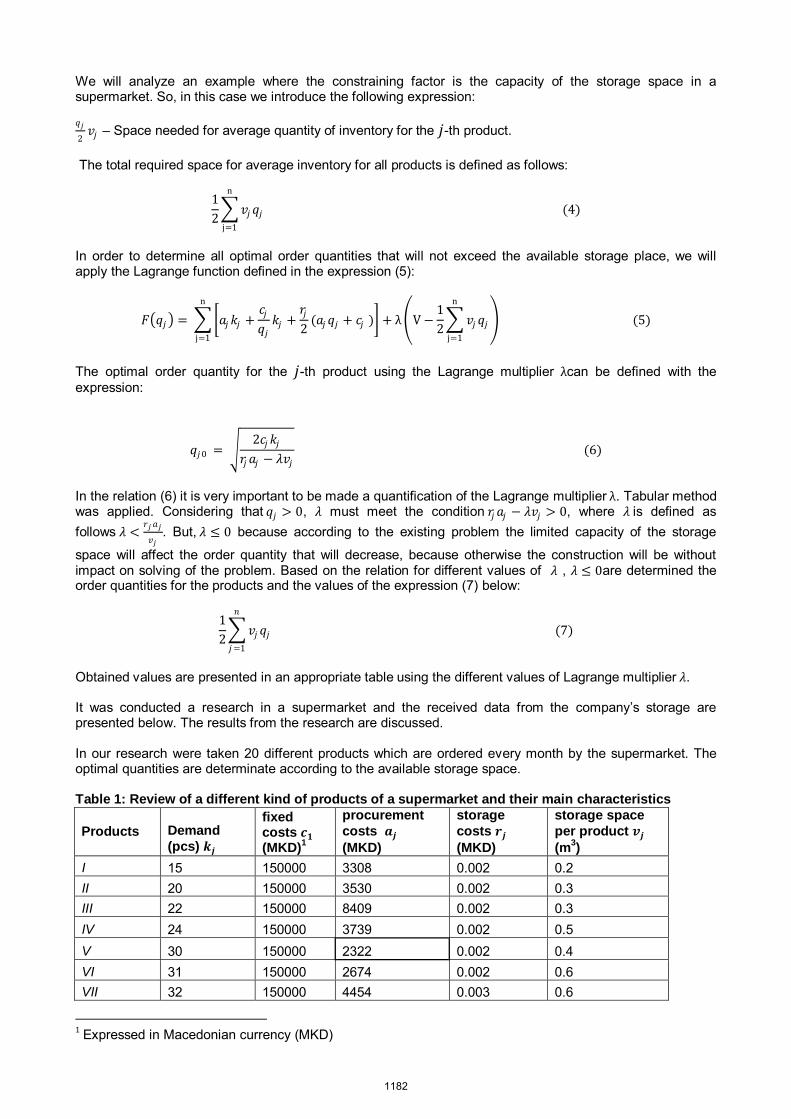
We will analyze an example where the constraining factor is the capacity of the storage space in a supermarket. So, in this case we introduce the following expression: 𝑞𝑗

2𝑣𝑗 – Space needed for average quantity of inventory for the 𝑗-th product.

The total required space for average inventory for all products is defined as follows:

1

2 𝑣𝑗𝑞𝑗

n

j=1

(4)

In order to determine all optimal order quantities that will not exceed the available storage place, we will apply the Lagrange function defined in the expression (5):

𝐹 𝑞𝑗 = 𝑎𝑗𝑘𝑗 +𝑐𝑗𝑞𝑗𝑘𝑗 +

𝑟𝑗2

(𝑎𝑗𝑞𝑗 + 𝑐𝑗 ) + λ V−1

2 𝑣𝑗𝑞𝑗

n

j=1

n

j=1

(5)

The optimal order quantity for the 𝑗-th product using the Lagrange multiplier λcan be defined with the expression:

𝑞𝑗0 = 2𝑐𝑗𝑘𝑗

𝑟𝑗𝑎𝑗 − 𝜆𝑣𝑗 (6)

In the relation (6) it is very important to be made a quantification of the Lagrange multiplier λ. Tabular method was applied. Considering that 𝑞𝑗 > 0, 𝜆 must meet the condition 𝑟𝑗𝑎𝑗 − 𝜆𝑣𝑗 > 0, where 𝜆 is defined as follows 𝜆 <

𝑟𝑗 𝑎𝑗

𝑣𝑗. But, 𝜆 ≤ 0 because according to the existing problem the limited capacity of the storage

space will affect the order quantity that will decrease, because otherwise the construction will be without impact on solving of the problem. Based on the relation for different values of 𝜆 , 𝜆 ≤ 0are determined the order quantities for the products and the values of the expression (7) below:

1

2 𝑣𝑗𝑞𝑗

𝑛

𝑗=1

(7)

Obtained values are presented in an appropriate table using the different values of Lagrange multiplier 𝜆. It was conducted a research in a supermarket and the received data from the company’s storage are presented below. The results from the research are discussed. In our research were taken 20 different products which are ordered every month by the supermarket. The optimal quantities are determinate according to the available storage space. Table 1: Review of a different kind of products of a supermarket and their main characteristics

Products Demand

(pcs) 𝒌𝒋

fixed costs 𝒄𝟏 (MKD)

1

procurement

costs 𝒂𝒋 (MKD)

storage

costs 𝒓𝒋 (MKD)

storage space

per product 𝒗𝒋 (m

3)

I 15 150000 3308 0.002 0.2 II 20 150000 3530 0.002 0.3 III 22 150000 8409 0.002 0.3 IV 24 150000 3739 0.002 0.5 V 30 150000 2322 0.002 0.4 VI 31 150000 2674 0.002 0.6 VII 32 150000 4454 0.003 0.6

1 Expressed in Macedonian currency (MKD)

1182

VIII 35 150000 14315 0.003 0.6 IX 38 150000 12103 0.003 0.5 X 42 150000 5040 0.002 0.9 XI 44 150000 15523 0.003 0.5 XII 46 150000 44850 0.004 0.7 XIII 50 150000 22750 0.004 0.9 XIV 51 150000 48705 0.004 0.9 XV 53 150000 6360 0.002 1.2 XVI 55 150000 14443 0.003 1.1 XVII 57 150000 11617 0.003 1 XVIII 59 150000 15611 0.003 1.1 XIX 60 150000 14440 0.003 1.2 XX 61 150000 25705 0.004 1.2

The Lagrange multiplier 𝜆 is taken as an appropriate for the values of 𝑞𝑗0 if their common volume is closest to the constraint below:

1

2 𝑣𝑗𝑞𝑗 ≤ V; 𝑞𝑗 > 0, j = 1,2,… , n

𝑛

𝑗=1

(8)

Based on the processed data given in the Table 1 is calculated the optimal order quantity for the 20th different products of the supermarket for an available storage place of 5000 m

3 and the calculation is given inthe Figure 2 in Microsoft Office Excel 2007.

Figure 1: Calculation of optimal order quantity for 20 different products in a limited storage space

1183

As the Figure 1 shows, based on assessments, we should calculate the values that are closing to the optimal quantity, which must be closest to the given available storage space of 5000 m3. In our case the optimal order quantity for each product is: 𝑞1 =809.1693124; 𝑞2 =897.7128481;

𝑞3 =619.3945056; 𝑞4 =941.6472309; 𝑞5 =1320.983601; 𝑞6 =1232.884922; 𝑞7 =824.190598; 𝑞8 =490.0917832;

𝑞9 =555.4427822; 𝑞10 =1058.978488; 𝑞11 =528.768245; 𝑞12 =276.6579312; 𝑞13 =403.4453962;

𝑞14 =279.4117813; 𝑞15 =1055.909306; 𝑞16 =607.2774956; 𝑞17 =687.9138062; 𝑞18 =605.7015394;

𝑞19 =633.4360052; 𝑞20 =418.7519525.

Their common volume is 4999,904566 m3 which not exceeds the available storage space of 5000 m

3.

The results from the Figure 1 are graphically presented and it is given a comment based on the obtained values.

From the graphic presentation on Figure 2 is conclude that as much as is smaller the value of Lagrange multiplier (𝜆 ≤ 0), the total required space for average quantity of inventory for all 20 products is decreasing and is closer to 5000 m3, which is the total available capacity of the storage of the supermarket.

The Series 1 show the total order quantity for all 20 products when there are changes in values in Lagrange multiplier when 𝜆 ≤ 0 and Series 2 show the total available storage space of 5000 m3.

As can be seen from the Figure 2 and Series 1 the order quantity for the first value for Lagrange multiplier (𝜆 = 0) is 5157.335839. Than we took another value for the Lagrange multiplier (𝜆 = −0,001) in order to decrease the occupied storage space and do not exceed the limited capacity of the warehouse of the supermarket. Next value for the Lagrange multiplier is 𝜆 = −0,002 where the order quantity decreases and amount 5157,072958. For 𝜆 = −0,055 the order quantity for all 20 products is 5150,128495. As the Lagrange multiplier decrease, so the order quantity is decreasing too. Therefore, our aim is to determine for which value of Lagrange multiplier the order quantity is optimal, so in our analysis the number of changed values for Lagrange multiplier (𝜆) was over 60 values. From the graphic presentation we can see that for the first few values of Lagrange multiplier, the order quantities are approximately same, until the order quantity decreases on a 5087,226963 for 𝜆 = −0,55.The last three values for Lagrange multiplier are very identical and all of them are very close to the amount of limited storage place. So, we calculated that for 𝜆 = −1,284,

the order quantity is most suitable to the limited amount of storage space of 5000 m3.

Figure 2: Graphic presentation of the optimal order quantity for determined values 𝝀 ≤ 𝟎

1184

In this case, when the optimal order quantity is determinate by the results from research, the minimum total order costs were also calculated with the Lagrange function given in the expression (5).

𝐹 𝑞20 = 𝑎𝑗𝑘𝑗 +𝑐𝑗𝑞𝑗𝑘𝑗 +

𝑟𝑗2

(𝑎𝑗𝑞𝑗 + 𝑐𝑗 ) + λ V−1

2 𝑣𝑗𝑞𝑗

n

j=1

n

j=1

(9)

Thus, the amount of minimum total order costs is 125.133 797, 2 MKD.

4. CONCLUSION

Optimal inventory management is very important for efficient working of the companies of the all industries. Inventories are one of the most expensive types of assets of the company, accounting for over 50% of the total invested capital. Inappropriate inventory management causes negative consequences, particularly high costs and big losses in profits of the companies.

There are many types of classification of inventory models. In this paper was elaborated the inventory model with constraints in capacity of the warehouse of a supermarket where there is a different kind of products. An important point of reference in this model is the estimate of the volume of storage space which is occupied by all products. Using this model the decision maker can easier determine the optimal order quantity which will have a volume that will not be larger than the available capacity, and will also result in a decreasing of total costs and setting them on minimum level. Today, in reality, companies have very little scientific support for their operations, so with our researches we can help them to improve operations and achieve positive results. Our suggestion is in the future trade companies to apply merging of the process of trade operations with process of the modeling, because the models thus created may enable prediction of the total costs of operations and the same to be minimized.

REFERENCES

Barkovič, D. (1997), Operacijska istraživanja, Ekonomski fakultet Osijek, Osijek, 379-383. Bonini, C. P., Hausman, W.H., & Bierman, H.Jr. (1997), Quantitative Analysis for Management, (9th edition),

Irwin/McGraw- Hill, Boston, 344-358. Choudhury, D. K., Saha, S., & Das, M. (2011). An inventory model with Lot Size Dependent carrying /

holding cost, Assam University Journal of Science & Technology: Psychical Sciences and Technology, 7(2), 133-136. Retrieved from http://www.inflibnet.ac.in/ojs/index.php/AUJSAT/article/view/544

Deterministic Inventory Models (DMI) (n.d). Retrieved March 15, 2014, from http://flash.lakeheadu.ca/~avantuyl/courses/oldcourses/OR_Lecture10a_Asampana.pdf

Dukič, G., Dukić, D., & Sesar, M. (2007). A model with storage limitation and simulated demand as fresh meat inventory management support, Poljoprivreda (Agriculture) Osijek, 13(1), 222-225. Retrieved from http://www.pfos.hr/~poljo/?q=vol-13-1-48

Felea, M. (2008). The role of inventory in the supply chain, Amfiteatru Economic, 10(24), 109-121. Retrieved from http://www.amfiteatrueconomic.ro/RevistaDetalii_EN.aspx?Cod=10

Pupavac, D. (1968), Matematičke metode u ekonomiji preduzeča, Beograd, 112-136. Ravindran, R. A. (2008), Operation research and management science, New York, 300-336. Reyes, M. P. (2005). A mathematical example of the two-echelon inventory model with asymmetric market

information, Applied Mathematics and Computation, 162(1), 257-264. Retrieved from http://www.sciencedirect.com/science/article/pii/S0096300304000864 Roumiantsev, S., & Netessine, S. (2007). What can be learned from classical inventory models: a cross – industry empirical investigation, Manufacturing & Service Operations Management, 9(4), 409-429. doi:10.1287/msom.1070.0166

Singh, Y. (2013). Optimal production policy for multi-product with inventory-level-dependent demand in segmented market, Yugoslav Journal of Operations Research, 23(2), 237-247.

doi: 10.2298/YJOR130220023S Su, S. M., & Lin, S. D. (2013). The Optimal Inventory Policy of Production Management, Engineering, 5(5A),

9-13. doi: 10.4236/eng.2013.55A002 Taha, H. A. (1995), Operations Research, (5th edition), Prentice Hall International, Singapore, 491- 494.Waters, C. D. J. (1949), Inventory control and management (2nd edition), London, 128-135. Retrieved from

http://en.bookfi.org/book/1409646

1185

OPTIMAL VEHICLE ROUTING IN THE OIL INDUSTRY

Jelena Golubović, Dragana Makajić-Nikolić, Nebojša Nikolić

University of Belgrade, Faculty of Organizational Sciences, gis@fon.bg.ac.rs

Abstract: The vehicle routing problem (VRP) has been solved as an optimization problem for more than fifty years. However, any real problem of this type has its own characteristics that should be included in a specific mathematical model. In this paper, we observe the vehicle routing problem in the oil industry. Based on the characteristics of a real company, an original mathematical model for supplying gas stations from multi-depots has been formulated. The routing problem is observed as a set covering problem and is formulated as a mixed integer programming (MIP) problem. Based on real data, an analysis of the optimal routes for different company policies on the organization of gas stations fuel supply has been done. Keywords: VRP, MIP, optimization, oil industry, multi-depot

1. INTRODUCTION

The vehicle routing problem (VRP) involves the design of a set of minimum-cost vehicle routes, originating and terminating at a central depot, for a fleet of vehicles that services a set of customers with known demands (Giosa, Tansini, & Viera, 2002). The VRP is so widely studied because of its applicability and its importance in determining efficient strategies for reducing operational costs in distribution networks. Today, exact VRP methods have a size limit of 50 - 100 orders depending on the VRP variant and the time-response requirements. Consequently, current research concentrates on approximate algorithms that are capable of finding high quality solutions in limited time, in order to be applicable to real life problem instances that are characterized by large vehicle fleets and affect significantly logistics and distribution strategies (Kumar & Panneerselvam, 2012). The pioneers of the VRP were Dantzig and Ramser. Their paper was concerned with the optimum routing of a fleet of gasoline delivery trucks between a bulk terminal and a large number of service stations supplied by the terminal. The shortest routes between any two points in the system were given and a demand for one or several products was specified for a number of stations within the distribution system. It was intended to find a way to assign stations to trucks in such a manner that station demands were satisfied and total mileage covered by the fleet was a minimum. A procedure based on a linear programming formulation was given for obtaining a near optimal solution (Dantzig & Ramser, 1959). A few years later, Clark and Wright (Clarke & Wright, 1964) improved the Dantzig/Ramser approach by proposing a heuristic. Following these two papers, many researchers studied algorithms and models for different versions of the VRP. Researchers are interested in studying the VRP for two reasons: its practical relevance and its difficulty. Lenstra and Rinnooy Kan (Lenstra & Rinnooy Kan, 1981) have analyzed the complexity of the VRP and concluded that practically all of the VRP problems are nondeterministic polynomial-time hard (NP-hard). VRP has many applications in real-world cases. Some applications are solidwaste collection, street cleaning, school bus routing, routing of salespeople and maintenance units, transportation of handicapped people, and so forth. The VRP can also be defined as the problem of designing least cost delivery routes from a depot to a set of geographically dispersed locations (customers) subject to a set of constraints (Daneshzand, 2011). An important characteristic of VRP is the homogeneity of the fleet of vehicles (Baldacci, Battarra, & Vigo, 2008). In this paper, we observe the heterogeneous fleet of vehicles. Also, the number of depots makes great difference in modelling and solving VRP (Crevier, Cordeau, & Laporte, 2007). Our problem involves the multi-depot from which the demand could be met. Fundamental components of the VRP are road network, customers, depots, vehicles, and drivers. To make different versions of VRP, different constraints and situations can be imposed on each component, and each of them can be supposed to achieve particular objectives (Toth & Vigo, 2002). Basic variants are capacitated VRP (CVRP), distance-constrained and capacitated VRP (DCVRP), VRP with time window (VRPTW), VRP with backhauls (VRPB), VRP with pickup and delivery (VRPPD), and any combination of these variants.

1186

This paper is related to the problem of optimal vehicle routing of an oil company in the Republic of Serbia. In the oil industry, the delivery of petroleum products can be divided in two parts (Sear, 1993): the transport of the first type, which is done through pipelines or railway, that includes transportation from refineries to storage depots; and the transport of the second type that includes transportation from storage depots to gas stations, and is done mostly by tanks. The subject of this paper is the other type of transport that includes a network of gas stations, which are being supplied via tanks from several storage depots.

This paper consists of five parts. After the introductory part, in the section two, the characteristics of the observed routing problem in the oil industry will be described. In the third section, we present the original MIP mathematical model that includes the basic characteristics of the routing problem in the observed company, and in the fourth, the results of the experiments are presented. Concluding remarks and directions for further work are given in the section five.

2. PROBLEM DESCRIPTION

The observed oil company supplies a network of over 300 gas stations from multi-depots. Each of these stations has a specific demand for petroleum products, and the delivery is done once their level falls under a certain limit. In the depots, tanks are assigned to transport the designated derivative, and the speed of supplying the gas station with the missing quantity depends on the demand for it, the distance between the station and the storage depot, as well as on the driving speed of the assigned tank.

Vehicle routing problem in the oil industry has certain particularities. The demand for derivatives fluctuates depending on the season, so the companies have a number of vehicles at their disposal during longer periods, and during seasonal peaks they outsource the missing vehicles. At the same time, oil companies use their vehicles for third party deliveries in return for a certain compensation, and this further complicates the formulation of the problem. It is necessary to take into account the existence of a window of time during which it is possible or, however, prohibited to deliver petroleum products.

Considering the nature of the goods being transported, it is impossible to transport together two different types of products due to their physicochemical characteristics. Based on this fact, the types of vehicles in the oil companies have been classified. It is also important to mention a series of regulations related to the transportation of hazardous matters and their manipulation, which are specific compared to the traditional problems. Once we take into consideration numerous existing limitations and assumptions, this problem presents a challenge for every oil company primarily due to data collection problems, the creation of the model and its dimension, and finally because of the difficulties with the implementation of the solution and maintenance over time.

In this paper, only some of the characteristics of the routing problem in the observed company will be considered. Given that the capacity of the vehicles varies, multi-depot CVRP will be used in the paper, whereas the maximum capacity for each tank will be defined. It should be noted that the tanks are never completely filled which will also be taken into account when defining the maximum capacity of the vehicle. Only the most common derivatives at the gas stations will be considered, such as petrol and diesel, as well as the vehicles intended for their transport. The basic assumption was that the demand at a gas station is met entirely by only one vehicle, but later this assumption was extended by the possibility of supplying one gas station from multi-depots. Two depots were considered, as well as their respective gas stations, while some routes, which implicated that the demand of one gas station could be met by only one or both depots, were also predefined.

Therefore, the observed problem has the following characteristics: - More storage depots; each of them owns a certain number of vehicles of different capacity at

disposal; - Large number of gas stations; some of them may be supplied from only one, while others may be

supplied from a variety of storage depots; - Limited maximum length of the route that complies with legal regulation and consists of time spent

driving between storage depots and gas stations and the retention time at the gas station; - Maximum and minimum capacities of the vehicle. Due to technical limitations, the gases that are

produced during transport, etc., the vehicle cannot be filled to the brim but there is a minimum level of the tank that must be filled for the safety of the journey;

Thus, the routing problem observed in this paper is a multi-depot capacitated VRP with heterogeneous fleet of vehicles. For the problem described, an original MIP mathematical model has been formulated. For given

1187

demands of gas stations, this model provides a set of routes and vehicles used for the routes in order to meet this demand with minimum total mileage. 3. MODEL FORMULATION An approximate approach was chosen in the modelling of the observed problem, meaning that the routing problem was formulated as a set covering problem. It is more common in the literature that the routing problem is modelled as a set partitioning problem (Kumar & Panneerselvam, 2012). Nevertheless, in this paper, by introducing an additional variable, it was achieved that one gas station could belong to several optimal routes, and that the retention time at the station counts only for the route on which the vehicle supplies the gas station. Thus, the observed problem becomes a set covering problem. One of the advantages of the approach used in this paper is that fewer routes need to be predefined than in the set partitioning approach. More precisely, when one feasible route is defined in the set partitioning approach, it is also necessary to define its sub-routes in order to insure obtaining feasible solutions. In the set covering approach it is not necessary to define sub-routes. Another advantage is that this way it is possible to gain solutions by which one gas station can be supplied by several vehicles. Once the vehicle routing problem is formulated as a set covering problem, we start from the predefined routes that could be used for supplying gas stations with petroleum. Among the predefined routes, those which cover all gas stations with demand and which have minimal total length (mileage) are chosen. The basic characteristic of this approach is that the quality of the obtained solution depends on the number and the quality of predefined routes. However, this approach allows faster solving, namely, less computational time needed for obtaining a solution. The following notation was used to formulate a mathematical model: Sets: V - set of available vehicles in all depots R - set of predefined routes that include all depots B - set of gas stations Parameters:

js - length of the j-th route in kilometers, j R ,

kp - the demand of the k-th gas station, k B ,

1 0

0 0

ifif

k

k

k

pd

p – parameter that defines whether there is a demand on the k-th gas station, k B

1 - -

0

if the th gas station is on the th routeotherwisekj

k ja , ,k B j R ,

1 - -

0

if the th vehicle belongs to the depot from which it departs on the th routeotherwiseij

i jm , ,i V j R ,

jt - traveling duration on the j-th route in minutes, j R

z - vehicle retention time at the gas station in minutes

tr - maximum allowed retention time of the vehicle on route in minutes min

iq - minimum capacity of the i-th vehicle, i V

1188

max

iq - maximum capacity of the i-th vehicle, i V

Variables:

1

0

if the - th vehicle is moving on the - th routeotherwiseij

i jx , ,i V j R

1

0

if the - th vehicle supplies the - th gas stationotherwiseik

i ky , ,i V k B

Using the introduced notation, the following mathematical model was formulated:

(min) j ij

i V j R

s x (1)

s.t.

1,ij

j R

x i V (2)

,ik k

i V

y d k B (3)

min 0,k ik i ij

k B j R

p y q x i V (4)

max ,k ik i

k B

p y q i V (5)

0, ,kj ij ij ik

j R

a x m y i V k B (6)

(1 ) , ,kj ij ik j ij

k B

a m y z t M x tr j R i V (7)

The objective function (1) minimizes the total mileage that all the vehicles used for supplying will cross. The first constraint (2) provides that one vehicle uses at most one route, and the constraint (3) provides that the demand at each gas station be fully met. The constraints (4) and (5) refer to the minimum and maximum vehicle capacity that must be reached and must not be exceeded. The variables ijx and iky are connected by constraints (6) and (7). Constraint (6) refers to the following: if there is a demand on the k-th gas station and if it is met by the i-th vehicle (i.e., if 1iky ), then it applies that the i-th vehicle needs to go along the j-

th route (i.e., that 1ijx ). The constraint (7) ensures that the total amount of time the vehicle will spend along the route will not be longer than the maximum time allowed, where parameter M is a very large number.

It is important to mention here that the manner in which the variable iky has been defined, that is, as a binary variable, implies that one gas station could only be supplied by one vehicle. If it is allowed that one gas station is supplied by several vehicles, the mathematical model remains the same while the variable iky

needs to be defined as a continuous variable as follows:

iky – percentage of the k-th gas station demand that is met by the i-th vehicle, 0 1iky , ,i V k B .

1189

4. NUMERICAL RESULTS The implementation of the mathematical model will be illustrated with a real example of an oil company. The observed problem involves two of the five depots which the company has at its disposal (depot I and the depot II). Depot I has 9 vehicles of different capacity, and depot II has 17 vehicles, also of different capacity. A total of 172 routes to 100 gas stations were predefined, out of which 99 routes start from depot I, and 73 routes from depot II. It is possible to transport fuel to 66 gas stations from depot I, and to 45 from depot II. In addition, it is possible to supply 11 gas stations from both depots. In accordance with legal regulations, the maximum amount of time which a vehicle can spend on the route is limited to 9 hours. As it was already mentioned, this amount of time consists of the time spent on the road and the retention time. Based on the consultations with company’s employees, it has been concluded that the average retention time at the gas station is 45 minutes: 30 minutes for fuel dispensing, and 15 minutes for filling in the documentation. The other parameters of the problem, such as the names of gas stations, their demand and tank capacities, have not been revealed due to data confidentiality. The following three scenarios have been analyzed: Scenario 1: Each gas station must be fully supplied from one tank. The minimum tank capacity is limited

to 25%. Scenario 2: Gas stations must also be supplied from one tank. The minimum tank capacity is limited to

30%, which corresponds better with the real situation in the company. Scenario 3: It is allowed that the gas station be supplied from multiple tanks, or more precisely, multiple

routes. This is achieved once the variable iky becomes continuous. The minimum tank capacity is limited to 30%.

In all three scenarios there is a demand on 51 of 100 gas stations. The effective capacity was taken as the upper limit of the tank capacity, that is, the percentage of the tank capacity that must remain empty was subtracted from the total capacity. Table 1 shows the results of all three scenarios. For each scenario the mathematical model has been implemented and solved using GNU Linear Programming Kit (GLPK), a software for solving MIP problems. Table 1: Results of the optimization Performances Scenario 1 Scenario 2 Scenario 3 Total mileage (km) 3239.8 3242.2 3242.2 Number of routes from depot I 9 9 9 Number of routes from depot II 10 10 10 Capacity usage 25-98% 30-100% 30-100% Total time on the routes 5542 5546 5636 The first row of the table 1 shows total mileage that all vehicles which participate in the supply of gas stations cross. The second and third rows refer to the number of routes, that is, the number of vehicles, from depot I and depot II. In the fourth row the range of capacity utilization of used tanks has been shown. The last row refers to the total time (in minutes) that all vehicles which participate in the supply spend on the routes (on the road and at gas stations). Based on the total mileage, the number of vehicles (routes) and time spent on routes, scenario 1 is the most profitable one for the observed company. However, this solution can only be applied if the lower limit of the capacity utilization which is 25% is acceptable. Optimal routes from scenario 2 differ from optimal routes in scenario 1, but the total number of routes is equal and the optimal value of the objective function is slightly inferior: the total mileage is only 2.4 kilometers longer. Total amount of time that vehicles spend on routes is only 4 minutes longer. Based on the obtained results, we can conclude that the company should not risk the loss by allowing that the vehicles be filled less than the safe limit of 30% tank capacity.

1190

The optimal objective function value and the route in Scenario 3 are the same as in Scenario 2. However, by Scenario 3, two gas stations will be supplied by two vehicles. 44.5% of a gas station demand will be met by one vehicle that departs from the depot I and 55.5% by the second vehicle that also departs from depot I. In the case of another gas station, 25.6% of the demand will be met by one and 74.4% of demand by the other vehicle. In this case, both vehicles also depart from the depot I. The consequence of such satisfaction of the demand is that the total retention time on routes prolongs for 90 minutes because it includes two stops at the two gas stations. In further research, the retention time will be seen as a variable value that depends on the amount of fuel to be dispensed at the gas station.

For given input data, Scenario 3 proved to be the most inadequate supplying type. Nevertheless, in the general case, allowing one gas station to be supplied by several vehicles could provide a solution with fewer routes than when this is not enabled. Fewer routes mean hiring a reduced number of vehicles and drivers, hence the lower supply costs.

5. CONCLUSION

The subject of this paper was the vehicle routing problem in the oil industry. In addition to the theoretical focus, this paper provides an overview of current issue in real oil company and the characteristics of vehicle routing problem in the Petroleum Industry of Serbia. On that basis, and in accordance with the information, an original MIP mathematical model was created. Vehicle routing problem was observed as a set covering problem.

The aim of this paper was to present a solution for one part of the complex vehicle routing problem in the real oil company, which would set the basis for the introduction of scientific methods that would allow solving this problem in the company. And as a result of "what -if" analysis, guidelines should be derived that will indirectly lead to cost reductions in the chain of gas stations supply with petroleum products.

REFERENCES

Baldacci, R., Battarra, M., & Vigo, D. (2008). Routing a heterogeneous fleet of vehicles. ,. In, The Vehicle Routing Problem: Latest Advances and New Challenges. New York, US, Springer, 3-27

Clarke, G., & Wright, J. V. (1964). Scheduling of vehicles from a central depot to a number of delivery points. Operations Research, 568-581.

Crevier, B., Cordeau, J.-F., & Laporte, G. (2007). The multi-depot vehicle routing problem with inter-depot routes. European Journal of Operational Research, 176(2), 756-773.

Daneshzand, F. (2011). The Vehicle-Routing Problem. In Z. R. Farahani, S. Rezapour, & L. Kardar, Logistics Operations and Management (pp. 127-153). London: Elsevier.

Dantzig, G. B., & Ramser, J. H. (1959). The Truck Dispatching Problem. Management Science, 80-91. Giosa, I. D., Tansini, I. L., & Viera, I. O. (2002). New assignment algorithms for the multi-depot. Journal of

the Operational Research Society, 977-984. GLPK http://www.gnu.org/s/glpk/ Kumar, S. N., & Panneerselvam, R. (2012). A Survey on the Vehicle Routing Problem and Its Variants.

Intelligent Information Management, 66-74. Lenstra, J. K., & Rinnooy Kan, A. G. (1981). Complexity of vehicle routing and scheduling problems.

Networks, 221-227. Sear, T. N. (1993). Logistics Planning in the Downstream Oil Industry. The Journal of the Operational

Research Society, 9-17. Toth, P., & Vigo, D. (2002). The Vehicle Routing Problem. Philadelphia: SIAM Monographs on Discrete.

1191

EFFECTIVENESS DETERMINATION OF HIGHER EDUCATION USING LINEAR PROGRAMMING

Tatjana Atanasova-Pacemska1, Riste Timovski2

1Associate professor, Faculty of Computer Sciences, Goce Delcev University in Stip, Republic of Macedonia, tatjana.pacemska@ugd.edu.mk

2Head of E-Index department, Rector’s cabinet, Goce Delcev University in Stip, Republic of Macedonia, riste.timovski@ugd.edu.mk

Abstract: Higher education presents main engine of society’s overall progress and development. The producers of the knowledge and future progressive force in all sectors of today’s living are personified in the Universities. As generators of academic individuals, it is important to achieve high level of educated and qualified students/future employees that will be able to fit in the real sector and contribute to the collective/personal live. To accomplish that, resources investments are necessary to be made by the Universities. The question is how to organize the resources in order of efficient production of high qualified future academic individuals. Moreover, in cases of inefficiency detection, the question is what is necessary to be done for improvement. This paper shows concrete linear programming technique application called DEA (Data Envelopment Analysis), used for measuring the efficiency of the University study program, who through its real implementation represents a basic generator of knowledge. Keywords: Linear Programming, Data Envelopment Analysis, Decision Making Units, Production levels, Composite units

1. INTRODUCTION

One of the main issues that companies’ and institutions’ management deals with is permanent optimization and improvement of its main process or production. Given the fact that solving of one problem in many cases can be done in more ways, it is important to find and implement the optimal between them. According to the literature that deals with the system optimization in terms of overall efficiency improvement, especially complex for analysis are service oriented institutions/organizations. Considering the fact that Universities in its basis aim to offer a service called quality education to the consumers personified in students, they can be analyzed precisely in this constellation.

Mathematical programming is special mathematical approach of selecting the best/optimal from the set of possible alternatives towards solving the problem. It assumes that it is possible to represent the problem as a mathematical model that reflects certain production function (more precisely, mathematical function). In this direction, resolution of the problem of optimization converges to determination of the optimal (minimum or maximum, depending on the nature of the model) value of the production function, having in mind all the limitations of the model/environment, represented in the limitation equations. In general, mathematical optimization implies that the production function and the accompanying limitation equations can be linear or nonlinear equations and/or inequalities. If the production function and all limitation equalities are represented in linear form, the mathematical optimization takes form of linear programming modelling and solvation. Nevertheless, some mathematical models have high complexity level and cannot be solved through known mathematical optimization models. Then, not optimal, but “good enough” solution is the subject, using orientation and heuristic models [1].

In context of the previously stated, the starting point for this work is how to build a model that portrays the knowledge and skills delivery very real, taking into account the fact that Universities are the knowledge and skills generators, in order to detect its pros and cons and certain, to propose concrete ways of improvement of this process. For this purpose, DEA (Data Envelopment Analysis) technique is used, starting from the fact that it’s nature of application offers very good possibility of model definition approach, as well as its mathematical processing and further discussion. Actually, this technique developed a new approach to the traditional cost / profit analysis and methods for efficiency measurement that enables policy-making through "learning from the best" and inducing theory from practice [2].

1.1. DEA (Data Envelopment Analysis)

There are several phases in LP appliance that have to be conducted: Definition of the problem and its mathematical formulation;

1192

Construction of the mathematical model; Finding the optimal solution of the model; Analysis of the results and sensitivity of the model, and Evaluation of the model and its implementation.

DEA as frontier analysis is designed for organization quality measurement and performance improvement, as main intention of the management. It is nonparametric non-statistical multi-criteria method that allows handling heterogeneous data. Based on LP, it operates with the term technological efficiency, defined as [3]:

(1) where input is presented as sum of the resources invested and output is presented as sum of the outcomes of the entity which efficiency is measured. The efficiency is noted as pareto efficiency if allocation of the resources (input and output) is such that better performances are not possible for the entity analyzed. Pareto efficient subject is the subject (entity) with best possible allocation of the resources. Here, it is impossible to improve the output without worsening the input.

DEA declares as effective those entities that produce a certain or more output parameters with fixed inputs or use the same or a smaller quantity of inputs to produce a certain output, compared with the other subjects within the same group being analyzed. The set that is subject of measurement is consisted of entities called DMUs (Decision Making Units) and they have to be homogenous. All DMUs have same inputs and outputs in different quantities. DMU can be institution, bank, human, production line, vehicle, part of vehicle etc. In this work, the subject/course of a concrete University’s study program is qualified as DMU. The mathematical model of DEA, starting from the definition of the efficiency of the k-DMU, in set of n DMUs with m inputs and s outputs given by [4]:

(2) Is defined as: Goal:

(3)

Given:

…

…

(4)

(5) (6)

where is j-th input in k-th DMU, is i-th output of the k-th DMU, are weights of the m inputs and are weights of the s outputs, both of the k-th DMU. DEA sets weights in such way – best way, to maximize the efficiency of every single DMU. So, the frontier is consisted of efficient DMUs with efficiency equals to 1. Every other DMU with efficiency below 1 is considered to be inefficient. Often, as in this paper, the dual DEA CCR model is used. It is represented with following equations: Find ; Having limitations:

(7)

(8) (9)

where index 0 represents each DMU that equations are solved for (in order to maximize its efficiency – observed DMU), lambdas are weighted coefficients that are used to represent the so-called composite DMU for each real DMU that will be located as inefficient. The composite DMU for each inefficient real DMU is consisted as sum of the ERS (efficiency reference set – efficient DMUs used for interpretation of the

1193

composite DMU for the observed real DMU) multiplied with its lambda coefficients. If A and B are efficient DMUs (m inputs, s outputs) and define the ERS set of observed inefficient C DMU, the composite DMU of C C’ can be interpreted as:

(10)

2. MATHEMATICAL MODEL

The model built is based on the fact that the delivery of knowledge, skills and competencies of students is conducted through practical implementation of curricula or course components during the study. DEA is particularly applied to service-oriented institutions and requires existence of a basic entity whose efficiency will be measured, with defined constellation of input resources invested and output outcome. Universities can be understood as subjects that deal with knowledge, skills and abilities delivery (basic function). Bearing this in mind, a mathematical model is conducted based on the need of measuring the efficiency level of the financial and other structural resources allocation by the University, with consideration of the achieved results in the process of knowledge, skills and abilities delivery to the students through the courses within a specific academic program. The resources are invested for each course and each course produces knowledge, skills and abilities. So, course / subject is the entity whose efficiency is measured, i.e. course as decision making unit (DMU): All inputs to the DMU are constellated so that their increase can reduce the efficiency of each study

course individually. In this manner, all output are considered to represent the outcome of the study program or each course practical implementation so that their increase will influence the increase of the efficiency of each study program individually.

Inputs of a single DMU are represented with: o Expenses and financial structure within each subject consumed on behalf of gross salaries

for professors and assistants that were engaged in the study program processing during years. Expenses are calculated in terms of gross salaries / expenses, with consideration of three months length (12 working weeks) of the semester (period of knowledge delivery) and the percentage of load in terms of number of students of the observed course and all students that the concrete person (teacher or assistant) covered during those three months. All increases and salary / expenses fluctuations are considered also. This data is gathered using the finance and human resources modules in ERP platform of the Goce Delcev University in Stip;

o Expenses and financial structure within each subject consumed on behalf of the equipment and inventory used for the concrete study program. This is done by calculation of the degree of utilization, i.e. the ratio of annual depreciation of computer equipment and inventory used, in accordance with their gross purchase price and the legislation. Percentage of load / utilization in terms of number of students of the observed course and all students that used the same equipment and inventory is considered, and

o Number of classes held, having in mind that classes load, forming study groups, classes and schedule organization is very important part in the process of overall course organization;

Outputs of a single DMU are represented with: o Index of the level of contribution of each course in skills, competencies and knowledge

delivery, prescribed with the accreditation elaborate of the study program (IP-KKV). Massive survey was realized at representative sample of 28 (of total of 88 students graduated at the study program), that generated indexes’ values, and

o Index of the quality of skills, competencies and knowledge delivered (IPKS-KKV) through the study program. This parameter, represented by the average grade of each course is calculated using the reporting module of the student information system of Goce Delcev University, fully automated for students’ e-administration.

1194

The model is shown in figure 1:

Figure 1. DEA Model: Course as DMU / Input = resources invested / Output = knowledge produced

3. CALCULATION, RESULTS AND DISCUSSION

Considering the above elaborated model and approach, table 1 shows the numerical side of it:

Table 1: Input / Output data Number

of classes

held

Expenses for equipment and

inventory

Expenses for professors and

assistants DMUs / Courses IPKKV IKPSKKV

24 28737,71 83066,86 English language 1 3,571 9,022 168 31190,88 122253,1 Electrical engineering 3,910 7,818 252 28737,71 87609,05 Math 1 3,928 7,170 168 31190,88 105634,6 Programing 4,267 6,852 24 25154,8 79832,87 English language 2 3,571 8,816 252 24766,98 101473,2 Linear algebra 3,875 7,556 252 27093,87 101473,2 Math 2 3,982 7,079 168 27093,87 107276,6 Objective programing 4,267 7

108 31979,06 36434,47 Probability and statistics 3,785 6,943

96 31979,06 78218,35 Digital logic 4,285 7,113 60 218481,7 51455,4 Operational systems 3,875 7,704 96 218481,7 131314 Software processes 3,964 7,295

96 218481,7 117407,6 Data structures and algorithms 4,25 6,954

96 154104,2 187273,8 Computer architecture 3,678 7,147 96 227342,5 62070,34 Data bases 4,321 7,318 72 118954,8 65492 Internet programing 4,339 7,238 72 12381,86 62527,75 Microprocessors 3,571 6,795

72 13413,68 64872,67 Software analysis and modeling 3,928 7,125

48 128867,7 65273,13 Graphics and visualization 4,160 8,170

72 128867,7 95668,31 Multimedia 3,982 7,693 72 87132,91 64428,28 Visual programing 4,339 7,056 72 7203,188 90306,62 Intelligent systems 4,142 7,693

72 7536,731 67004,76 Distant learning systems 3,196 7,602

72 7536,731 57935,99 Software projects management 3,821 7,011

1195

The model has been applied on 24 subjects of the study program of Informatics at the Faculty of Computer Sciences, generation of students 2007/2008. The numerical model is processed in Open Source DEA software application (http://www.opensourcedea.org/index.php?title=Open_Source_DEA). The results of the subjects’ efficiency measurement are given in table 2: Table 2: Courses efficiency

DMU / Subject Efficiency DMU / Subject Efficiency

English language 1 1 Data bases 0,856 English language 2 1 (ERS=6) Digital logic 0,82

Probability and statistics 1 (ERS=12) Multimedia 0,684 Operating systems 1 (ERS=2) Math 1 0,59

Graphics and visualization 1 (ERS=10) Linear algebra 0,566

Intelligent systems 1 Data structures and algorithms 0,558

Distant learning systems 1 Objective programming 0,551 Software projects

management 1 (ERS=16) Programming 0,548

Visual programming 0,98 Math 2 0,538 Software analysis and

modeling 0,958 Electrical engineering 0,494

Internet programming 0,942 Software processes 0,487 Microprocessors 0,893 Computer architecture 0,375

Courses with efficiency = 1 are noted as relativly efficient courses and are set of representative courses for the courses with efficiency bellow 1, noted as inefficient courses. Most efficient courses are used in most of the cases of composite courses. In general, composite unit (in this case, the course) is the unit that DEA propose for each inefficient unit towards its optimization. Each inefficient unit has its own composite unit, as its example of best input / output allocation. The composite units are generated as the sum of the detected and specific (diferent for each inefficient DMU) ERS units and lambda corresponding coefficients, known as production levels. Courses that are bold in table 2 are noted as entities consisting Efficiency Reference Set – ERS, used in creating composite courses. ERS = X notes the number of times this course is used in creation of composite units for the inefficient detected courses. This defines Graphics and visualization and Probability and statistics as best efficient subjects, and Software processes and Computer architecture as subjects with worst resource invested and outcome results constellation. Table 3 defines all inefficient courses in terms of definition of their composite DMUs (that are “on the frontier” and are what they “should be like”).

Table 3. Production levels of inefficient DMUs

COMPOSITES

EFFICIENCY REFERENCE SET

English language 2

Probability and statistics

Operating systems

Graphics and visualization

Software processes management

INEFFICIENT COURSES

LAMBDAS / PRODUCTION LEVELS

Electrical engineering

0,086514754 0,230296305 0 0 0,778229001

Math 1 0 0,375590319 0 0 0,655957254 Programming 0 0,325830999 0 0,009357358 0,783848429 Linear algebra 0 0,240252428 0 0 0,839884745 Math 2 0 0,2745388 0 0 0,770090534 Objective programming 0 0,265867267 0 0 0,853439903

Digital Logic 0 0,05593835 0 0,135779195 0,918245408

Software processes 0,080624363 0 0 0,804743829 0,085840258

1196

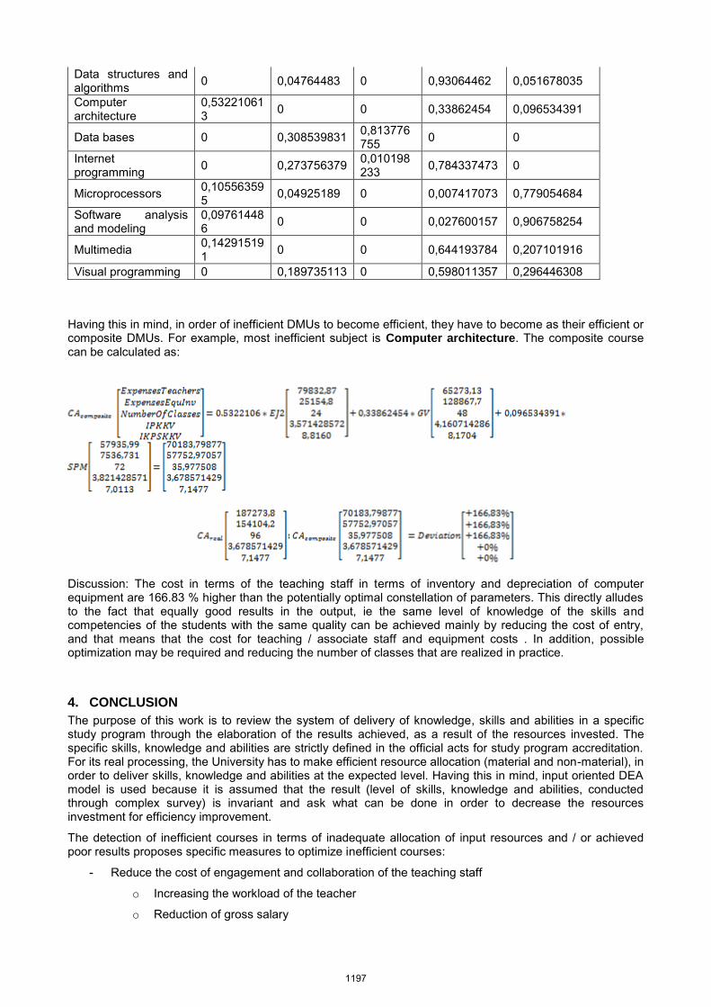
Having this in mind, in order of inefficient DMUs to become efficient, they have to become as their efficient or composite DMUs. For example, most inefficient subject is Computer architecture. The composite course can be calculated as:

Discussion: The cost in terms of the teaching staff in terms of inventory and depreciation of computer equipment are 166.83 % higher than the potentially optimal constellation of parameters. This directly alludes to the fact that equally good results in the output, ie the same level of knowledge of the skills and competencies of the students with the same quality can be achieved mainly by reducing the cost of entry, and that means that the cost for teaching / associate staff and equipment costs . In addition, possible optimization may be required and reducing the number of classes that are realized in practice.

4. CONCLUSION

The purpose of this work is to review the system of delivery of knowledge, skills and abilities in a specific study program through the elaboration of the results achieved, as a result of the resources invested. The specific skills, knowledge and abilities are strictly defined in the official acts for study program accreditation. For its real processing, the University has to make efficient resource allocation (material and non-material), in order to deliver skills, knowledge and abilities at the expected level. Having this in mind, input oriented DEA model is used because it is assumed that the result (level of skills, knowledge and abilities, conducted through complex survey) is invariant and ask what can be done in order to decrease the resources investment for efficiency improvement.

The detection of inefficient courses in terms of inadequate allocation of input resources and / or achieved poor results proposes specific measures to optimize inefficient courses:

- Reduce the cost of engagement and collaboration of the teaching staff

o Increasing the workload of the teacher

o Reduction of gross salary

Data structures and algorithms 0 0,04764483 0 0,93064462 0,051678035

Computer architecture

0,532210613 0 0 0,33862454 0,096534391

Data bases 0 0,308539831 0,813776755 0 0

Internet programming 0 0,273756379 0,010198

233 0,784337473 0

Microprocessors 0,105563595 0,04925189 0 0,007417073 0,779054684

Software analysis and modeling

0,097614486 0 0 0,027600157 0,906758254

Multimedia 0,142915191 0 0 0,644193784 0,207101916

Visual programming 0 0,189735113 0 0,598011357 0,296446308

1197

o Option for freelance engagement of staff with less financial burden

- Reduce the cost of equipment and inventory

o Purchase of equipment and inventory at a lower purchase price

o Increasing utilization of the unit (in terms of number of students)

o Increasing the rate of depreciation

- Reducing the number of realized lectures and tutorials

o Reduction and convergence of matter in fewer lectures

o Pipe classes for lectures and tutorials

o Reducing the number of students’ groups

o Intervention within the study programs / change relevant parameters

For more accurate investigation, it is possible to do an extension of the model by increasing the parameters that are not taken into account in this case, according to the perception of the management of the University. DEA allows that in order of geenration even more appropriate and realistic model.

REFERENCES Taha, Hamdi A., (2007). Operational research, Introduction. New Jersey: Pearson Education, Inc. Charnes, A., Cooper, W.W., Lewin, L. A., Seiford, M. L., (1994). Data Envelopment Analysis, Theory,

Methodology and Applications. Norwell, Massachusetts: Kluwer Academic Publishers. Charnes, A., Cooper, W.W., Rhodes, E., (1978). Measuring the Efficiency of Decision Making Units.

Amsterdam: North-Holland Publishing Company. Cooper, W.W., Seiford, M. L., Tone, K., (2007). Data Envelopment Analysis, A Comprehensive Text with

Models, Applications, References and DEA-Solver Software, Second Edition. New York: Springer. Aronson, E. J., Zionts, S., (1998). Operation Research: Methods, Models, and Applications. Westport,

Connecticut: Quorum Books. Breirerova, L., Choudhari, M., (1996). An Introduction to Sensitivity Analysis. Massachusetts :Massachusetts

Institute of Technology. Cooper, W. W., Seiford, M. L., Zhu, J., (2011). Data Envelopment Analysis: History, Models and

Interpretations. New York: Springer. Directorate General – Education and Culture, European Commission, (2009). ECTS Users’ Guide. Office for

Official Publications of the European Communities. Yang, Y., Ma, B., Koike, M., (2000). Efficiency – Measuring DEA Model for Production System with k

Independent Subsystems. Journal of the Operations Research, Society of Japan, Vol. 43, No. 3,

1198

MULTI-CRITERIA OPTIMIZATION OF THE MOST COMPETITIVE BANK IN MONTENEGRO SELECTION PROCESS

Rakočević Svetlana, Dragašević Zdenka, Glišević Nevenka University of Montenegro, The Faculty of Economics, Podgorica, rakocevic@ac.me University of Montenegro, The Faculty of Economics, Podgorica, zdenka@ac.me

University of Montenegro, The Faculty of Economics, Podgorica, nenacg5@yahoo.com ____________________________________________________________________________________ Abstract: Multi-Criteria Decision Making (MCDM) is one of the most prominent branches in decision-making process. It is applied in all those situations where there is a range of often conflicting criteria based on which an optimal decision is to be taken. It is the existence of a number of criteria that is a significant step towards the reality of problems that can be solved by applying MCDM methods. This paper presents a methodology of applying the AHP (Analytic Hierarchy Process) method in selecting the most competitive bank in the Montenegrin market. By reducing a complex decision making problem to comparing pairs of options and through a synthesis of obtained results, the AHP method enables reaching the most favorable decision.

Key words: decision making, multi-criteria decision making, banks, AHP method

1. INTRODUCTION

A transition process in Montenegro has instigated a reform of the financial sector. The reform has been aimed at providing security and stability of the financial system and boosting efficiency and profitability of the banking system. Reforms have yielded good results. New legislation has been passed, ownership transformation has been implemented, a new concept of bank management has been adopted and a supply of banking products has been increased.

Banks occupy a central position in a country’s financial system, due to both the function they perform and the financial potential at their disposal. Contemporary banks are multiservice financial institutions which, in addition to their primary functions, offer a wide range of financial products and services to their customers. The nature of their business is such that banks are market-oriented enterprises operating on principles of liquidity, safety and profitability, aimed at maximizing profit.

The main institution in charge of supervision and oversight of the financial services sector in Montenegro is the Central Bank of Montenegro, founded in March 2001. As an independent institution, the Central Bank is responsible for monetary policy, establishing and maintaining a sound banking system and an efficient payment system. In 2010, a new Law on the Central Bank of Montenegro was passed, based on the new Constitution of Montenegro. Pursuant to that law, the Central Bank has assumed responsibility for providing stability of the financial system, including the promotion and maintenance of a sound banking system and a safe and efficient payment system.

2. BANKING SYSTEM IN MONTENEGRO

Since 2007, the banking sector of Montenegro has comprised 11 commercial banks and six micro-financing institutions that have a license issued by the Central Bank. Within the Central Bank, there is a special department for the control of banks. This department reports on financial indicators of each bank and ensures that each bank maintains a minimum share of capital equity in relation to total assets, as stipulated by law. As part of measures aimed to strengthen the financial system, special attention has been devoted to enhancement and maintenance of banking system stability. In order to achieve that, the Central Bank continuously monitors and analyzes, and if necessary, undertakes corrective measures to strengthen corporate governance and risk management and to ensure further implementation of internationally accepted standards and business principles (BTI 2014, Montenegro country report).

Since the beginning of transition, the banking sector has gone through a substantial change. As the privatization of state-owned banks was one of the main items of banking sector recovery, primarily through foreign capital inflow, a share of foreign capital has increased significantly. The crisis, which hit the world in 2008, affected Montenegro mostly as a lack of trust. Fearful that problems from the 1990s may reemerge, a certain number of people began to withdraw their deposits from the banking system. However, as the crisis spread to the real sector, an increasing number of companies became insolvent and they slowly started to

1199

close and fall into bankruptcy. Since the second half of 2009, the situation has started to improve. Deposits have started to grow which is a sign of recovery and stability of a banking system. Profitability of the banking sector has made significant progress over the last decade. This is primarily due to a comprehensive reform of the banking sector, write-off of bad loans, privatization of state-owned banks, separation of commercial banks from the Central Bank, liberalization of interest rates, introduction of modern banking technology, expansion of loans etc., and opening banking sector to private and foreign units as well. Generally speaking, Montenegrin banking system has experienced a growing trend in profitability . Stability of the banking system is, among other things, reflected in parameters of liquidity and solvency of banks, and at the end of 2013, these parameters were above the stipulated level. Growth of 4.9%, as compared to the end of the previous year, in total loans and other receivables in the first six months of 2013, is not only the result of an increase in newly approved loans but is also partly fostered by changes in regulations and implementation of IAS as well, and in view of this banks returned a part of written-off loans and other receivables from off-balance sheet items. However, in spite of the efforts banks have undertaken to reduce the level of non-performing loans1 in the post-crisis period, continuity in growth of these loans has remained the biggest vulnerability of the banking sector and a potential source of risk to financial stability. Despite a moderate success attained by moving non-performing loans to parent banks’ balance sheets or by selling and/or restructuring loans, their upward trend has continued. At the end of July this year, non-performing loans and other receivables accounted for 17.8% of total loans and other receivables. A key challenge in 2014, just like in previous years, will be a reduction in volume of non-performing loans. A so called “Podgorički model” for voluntary restructuring of non-performing loans has been developed, and this model has received a full support of the Central Bank, the Ministry of Finance and the World Bank. It is a very complex project whose implementation requires passing lex specialis for its enforcement in practice. The project is aimed at improving the performance of solvent legal entities – companies and entrepreneurs – that are dealing with temporary liquidity problems, and by doing that – at providing banks performance boost, since banks are a pillar of stability and support of banking system recovery. The project will, in the long term, prompt positive impulses for triggering economic activities and consolidating real economy. Also encouraging is the fact that banks deposits grow, which leads to improved credit-to deposit-ratio. At the end of June 2013 the increase in deposits was 1.5%. Lending rates, both in 2012 and during 2013 were extremely high due to the high country risk premium, and thus more expensive fund sources, the upward trends of non-performing assets, risk rating and the general business climate. Due to limited access to resources, banks turned to domestic sources, secured by offering higher deposit rates, which resulted in higher interest margins. Figure 1 (Source: Financial statements of banks in 2013) shows the proportion of Montenegrin banks in the banking system of Montenegro measured by total assets. The Montenegrin Commercial Bank has the largest share and accounts for 20% (of total assets), followed by the NLB Bank with 17% and the Societe General Bank of Montenegro with 12%. Other banks account for less than 10%. Figure 2 (Source: Financial statements of banks in 2013) shows the share of banks in the banking sector in relation to the amount of loans given in 2013. The CKB (the Montenegrin Commercial Bank) comes first by this criterion as well with the share of 25%, followed suit by the NLB with 19% while the Societe General Montenegro is in the third place with 16%. Bank performance has traditionally been measured based on an analysis of financial indicators. The most common way of performing analysis is based on the criteria of liquidity, profitability, capital efficiency and adequacy, whereby different models of multi-criteria analysis can be used. This paper has employed the AHP (Saaty, 1993) model for the ranking of Montenegrin banks.

1 In compliance with the amended regulation, which came into force on January 1st 2013, a share of non-performing loans and other receivables is calculculated as a percentage of non-performing gross loans and other receivables, without interest and time limits, in total loans and other receivables.

1200

Figure 1. The share of banks in the banking sector of Montenegro – total assets

Figure 2.The share of banks in the banking sector of Montenegro – loans

3. AHP MODEL FOR BANK RANKING AND COMPARISON

In order to make an AHP model it is necessary to define the goal, criteria, sub-criteria and alternatives. The goal of this model is ranking of the banks in Montenegro from the best to the worst; the criteria have been divided into two groups – qualitative and quantitative. Quantitative criteria are financial ratios which display characteristics of certain bank performances. When choosing financial ratios in the model, the experience of many different experts in the field has been used (Yeh, 1996). Financial ratios are divided into four groups: liquidity, efficiency, profitability and capital adequacy. Within each group sub-criteria have also been defined. Liquidity sub-criteria are:

1) L1 = money + money equivalents + investments/total deposits;2) L2 = total approved loans/total deposits;3) L3 = Liquid assets/total assets

Efficiency sub-criteria are: 1) E1 = operational expenditures/operational income;2) E2 = provision costs/net interest rate income;3) E3 = operational income/total number of employees.

Profitability sub-criteria are: 1) P1 = Profit before tax/equity;2) P2 = Profit before tax/total assets;3) P3 = Profit before tax/operational income.

And for the last group – capital adequacy, the sub-criteria are: 1) C1 = total obligations/equity;2) C2 = equity/total loans;3) C3 = total deposits/equity.

Qualitative factors are owners’ support, the importance of a bank in the financial system of Montenegro (significance), management and the bank maturity. These criteria could not be described by any of qualitative methods, so we use verbal descriptions. Alternatives are represented by 7 Montenegrin banks.

In order to use this model for bank ranking, we need to determine the weights of the main criteria and sub-criteria, and then for each criteria at the bottom level of the hierarchy structure to define the intensities for the evaluation of the relevant bank performances. The weights of criteria and sub-criteria are calculated by the

1201

help of Super Decision software on the basis of the pairwise comparison of relative criteria and sub-criteria importance. For quantity criteria, the intensities are defined on the basis of the five-level scale of intensities (excellent, very good, good, satisfied, bad), which have been derived on the basis of the range in which their values have fluctuated. As for the qualitative criteria, we have used the same evaluation as in CAMELS method, so the intensity scale for each category has been generated. For example, the scale for owners support is defined as: excellent, very good, good, satisfied and bad; the importance of the bank as: excellent, very good, good, satisfied and small; the management: excellent, very strong, strong, average, weak and, finally, the maturity of the bank is assessed as: more than 10 years, from 5 to 10 years, and less than 10 years. CAMELS method has 5 levels for each criteria, but due to the deficiency of precise and quality information, it has not been possible to recognize some subtler levels, as can be performed by the examiners for the bank monitoring who are entitled to have access to all the necessary information. Structure of the AHP model for bank ranking and comparison is presented in Figure 3.

Goal

Quantitative criteria

EfficiencyLiquidity Profitability Capitaladequacy Support Significance Management

Qualitative criteria

E1 E2 E3

P1 P2 P3

A1 A2 A3

Bank1 Bank 7Bank 2 Bank 3 Bank 4 Bank 5 Bank 6

Maturity

L1 L2 L3

Figure 3. Structure of the AHP model for bank ranking and comparison

4. APPLICATION OF THE AHP METHOD FOR RANKING BANKS IN MONTENEGRO The banking sector in Montenegro consists of 11 banks. For the purposes of this study, seven banks2 with the largest market share have been analyzed. The data on the banks’ financial indicators date from 2013 and have been obtained from the annual financial statements. The values of financial indicators are presented in Table 2 while the values of the intensity of the quantitative criteria are shown in Table 3. The weights of criteria and sub-criteria are calculated by the help of Super Decision software on the basis of the pairwise comparison of relative criteria and sub-criteria importance. For quantity criteria, the intensities are defined on the basis of the five-level scale of intensities (excellent, very good, good, satisfied, bad), which have been derived on the basis of the range in which their values have fluctuated (Table 3). For the qualitative criteria, we have used the same evaluation as in CAMELS method, so the intensity scale for each category has been generated. Based on the data for the seven banks that were analyzed using the AHP model, a ranking list of banks has been obtained. A graphic illustration of the ranking list of banks is shown in Table 1 while Figure 4 shows the weights of certain quantitative and qualitative criteria.

Table 1. Graphical illustration of ranks

2 Names of banks known to authors

1202

Figure 4. Weights for quantitative and qualitative criteria Liquidity 0.41667 Efficiency 0.25000 Profitability 0.12500 Capital adequacy 0.20833 Owners’ support 0.1601 Importance 0.2008 Management 0.0160 Maturity 0.1000

From Table 1 it can be seen which rank is taken by each selected bank all the given criteria taken into account. In fact, in the overall ranking the best bank in Montenegro is Bank 1, Bank 3 is the runner-up, followed by Bank 4 and Bank 7. The last and the second last place are taken by Bank 5 and Bank 6, respectively.

Bank ranks according to individual criteria (liquidity, efficiency, profitability, capital adequacy and qualitative criteria) have been calculated in a similar manner if the purpose of the analysis is to find the best bank in terms of a single criterion. The banks can be ranked separately on quantitative and qualitative criteria.

When taking into account only quantitative criteria, the analysis can be carried out separately according to individual quantitative criteria, such as the liquidity criterion (Table 4), the efficiency criterion (Table 5), the profitability criterion (Table 6) and the capital adequacy criterion (Table 7).These tables show that Bank 1, which is ranked best in the overall rating, according to these criteria usually occupies the sixth position (according to the criteria of liquidity and efficiency), i.e., the fourth according to the criterion of profitability and the second according to the criterion of capital adequacy. When you look at the table that shows the ranking of the banks according to qualitative criteria (Table 8), we can note that the leading bank is Bank 1. Thanks to qualitative criteria, as well as a good position according to capital adequacy criterion, the bank is the first in the overall ranking. This information may be of interest for those making decisions on the selection of the most competitive bank.

1203

Table 2. Values of financial ratios Criterion

Alternative L1 L2 L3 E1 E2 E3 P1 P2 P3 C1 C2 C3

Bank 1 1.16 1.00 0.13 0.42 0.06 82.26 0.08 0.010 0.17 6.59 9.49 6.16

Bank 2 1.31 0.88 0.32 0.48 0.00 94.74 -0.32 -0.030 -0.52 9.38 1.12 7.75

Bank 3 1.28 1.07 0.15 0.36 0.00 84.19 0.14 0.016 0.23 7.81 0.83 6.49

Bank 4 1.53 1.29 0.15 0.35 0.00 106.87 0.15 0.017 0.22 7.85 0.58 5.55

Bank 5 2.08 1.76 0.14 0.46 0.00 70.56 -0.07 -0.013 -0.23 4.07 0.58 2.28

Bank 6 0.99 0.85 0.11 0.55 0.05 59.64 0.01 0.002 0.03 7.09 13.06 6.60

Bank 7 1.28 1.07 0.15 0.36 0.00 77.90 0.09 0.012 0.20 6.76 1.13 5.67

Criterion Max max max min min max max max max min max min

Best value 2.08 1.76 0.32 0.35 0.00 106.87 0.15 0.017 0.23 4.07 13.06 2.28

Worst value 0.99 0.85 0.11 0.55 0.06 59.64 -0.32 -0.030 -0.52 9.38 0.58 7.75

Table 3. Values of intensities Criterion L1 L2 L3 E1 E2 E3 P1 P2 P3 C1 C2 C3

Type max Max max min min max max max max min max min

Excellent (1.81 - 2.1) (1.51 -

1.8) (0.31-0.5) (0.3-0.36) (0.0-

0.009) (98-107) (0.15-0.18)

(0.015-0.018)

(0.21-0.25) (3 -4.5) (11.1-13) (0.0 - 2.5)

Very good (1.51-1.8) (1.31-1.5) (0.26-0.3)

(0.37-0.39)

(0.01-0.019) (92-97)

(0.11-0.14)

(0.011-0.014)

(0.17-0.20)

(4.51 - 6.5) (8.1-11) (2.51 -3.5)

Good (1.21-1.5) (1.11-1.3)

(0.21-0.25) (0.4-0.42)

(0.02-0.03) (84-91)

(0.07-0.10)

(0.007-0.010)

(0.11-0.16)

(6.51 - 7.5) (5.1-8) (3.51 -5)

Satisfied (1.1-1.2) (0.91-1.1) (0.16-0.2)

(0.43-0.46)

(0.04-0.05) (76-83)

(0.03-0.06)

(0.003-0.006)

(0.06-0.10) (7.51 - 9) (2.1-5)

(5.01 - 6.5)

Bad (0.61-1) (0.71-0.9) (0.1-0.15)

(0.47-0.56)

(0.06-0.07) (58-75) (0.0-0.02) (0.0-0.002) (0.0-0.05) (9.01-10) (0-2) (6.51 -8)

1204

Table 4. Liquidity criteria Table 5. Efficiency criteria Weights 0.11067 0.04611 0.06148

L1 L2 L3 Total Ranking Bank 1 0.5588 0.5706 0.3943 0.1124 6 Bank 2 0.6321 0.5004 1.0000 0.1545 2 Bank 3 0.6143 0.6098 0.4637 0.1246 5 Bank 4 0.7360 0.7353 0.4571 0.1435 3 Bank 5 1.0000 1.0000 0.4435 0.1840 1

Bank 6 0.4752 0.4846 0.3401 0.0958 7 Bank 7 0.6142 0.6060 0.4746 0.1251 4

Weights 0.0520 0.0404 0.0385 E1 E2 E3 Total Ranking

Bank 1 0.8411 0.0000 0.7697 0.0734 6 Bank 2 0.7320 1.0000 0.8866 0.1127 3 Bank 3 0.9900 1.0000 0.7878 0.1223 1

Bank 4 1.0000 0.0002 1.0000 0.0905 5 Bank 5 0.7657 1.0000 0.6603 0.1057 4 Bank 6 0.6383 0.0000 0.5581 0.0547 7 Bank 7 0.9793 1.0000 0.7290 0.1194 2

Table 6. Profitability criteria Table 7.Capital adequacy criteria Weights 0.0356 0.0119 0.0180

P1 P2 P3 Total Ranking Bank 1 0.5157 0.6013 0.7417 0.0388 4 Bank 2 -2.1179 -1.7654 -2.2362 -0.1366 7 Bank 3 0.9100 0.9147 1.0000 0.0613 2 Bank 4 1.0000 1.0000 0.9657 0.0649 1

Bank 5 -0.4504 -0.7867 -0.9728 -0.0429 6 Bank 6 0.0965 0.1057 0.1359 0.0071 5 Bank 7 0.6018 0.6863 0.8726 0.0453 3

Weights 0.0290 0.0499 0.0302 C1 C2 C3 Total Ranking

Bank 1 0.6170 0.7269 0.3703 0.0654 2 Bank 2 0.4338 0.0857 0.2942 0.0258 7 Bank 3 0.5212 0.0638 0.3516 0.0289 6 Bank 4 0.5180 0.0441 0.4111 0.0297 5 Bank 5 1.0000 0.0446 1.0000 0.0615 3 Bank 6 0.5741 1.0000 0.3455 0.0770 1

Bank 7 0.6016 0.0868 0.4023 0.0339 4

Table 8. Qualitative criteria Weights 0.1601 0.2008 0.0160 0.1000

Owners’ support

Importance Management Maturity Total Ranking

Bank 1 1 1 1 0.77 0.4539 1

Bank 2 0.55 0.77 0.77 0.55 0.3100 5 Bank 3 1 1 1 0.55 0.4319 2 Bank 4 1 0.77 1 0.55 0.3857 3 Bank 5 0.77 0.33 0.33 0.33 0.2278 7 Bank 6 0.55 0.55 0.55 0.55 0.2623 6 Bank 7 0.55 0.77 0.77 1 0.3550 4

5. CONCLUSION

One of the options for finding a model to measure bank performance is the control of the banks performed by the Central Bank. The control is a common interest of the Central Bank, capital owners and users of banking services. The Central Bank, as the institution in charge of monetary policy, performs control over the banks in order to be able to promptly react to potential problems and protect the interests of citizens and the entire economic system. The owners of capital in banks are more and more interested in establishing an efficient and effective system of internal control in order to ensure better competitiveness through identifying the causes of their inefficiency and taking preventive action to avoid them. From the perspective of consumers – users of banking services, supervision over banks is important to avoid the risk of doing business with high-risk banks.

In the modern-day business world, in order to make optimal decisions, it is necessary to analyze the problem in terms of multiple criteria. In such cases, it is possible to use methods of multiple criteria decision-making. The choice of method depends on a particular case and the aim of the decision-maker. Some of the known methods are: ELECTRA, PROMETHEE, DEA, CAMELS, VIKOR and AHP. In this paper we employed the AHP method, in order to rank the banks in Montenegro, based on defined criteria. The advantages of the AHP method are in the possibility of inclusion of qualitative criteria and in the fact that apart from overall ranking, the alternatives can be ranked according to individual criteria and sub-criteria, which is an advantage that is often critical when decision-makers decide to use the AHP method. Montenegrin banks have been ranked applying the AHP method on the basis of quantitative and qualitative criteria, and with the help of a software package Super Decision. Banks have been ranked according to the criteria of liquidity, efficiency, profitability, capital adequacy, equity support, the importance for the financial market in Montenegro, management and maturity. In the overall ranking the best bank in Montenegro in 2013 is Bank 1. This practical example, accompanied by data from the financial statements, has shown the benefits of the AHP method, and helped in determining the most

1205

competitive bank in Montenegro on the basis of several criteria relevant to the study, as well as in ranking the other banks.

REFERENCES

BTI (2014). Montenegro country report Caterino, N., Iervolino, I., Manfredi, G., Cosenza, E. (2009). Comparative analysis of multi-criteria decision

making methods for seismic structural retrofitting, Computer –Aided Civil and Infrastructure Engineering, 24.

Centralna Banka Crne Gore (2014). Preporuke vladi Crne Gore za ekonomsku politiku 2014. Dragašević, Z., (2010). Modeli višekriterijumske analize za rangiranje banaka, Doktorska disertacija, Ekonomski

fakultet Podgorica European Investment bank (2013). Banking in Central and Eastern Europe and Turkey Challenges and

Opportunities Fabris, N., Mitrović, M.(2012). Central Bank of Montenegro, Critical overview of Montenegro’s growth model,

East-West journal of economics and business, vol. xv – 2012, no 1 & 2 Feng, Y., Lu, H., Bi, K. (2004). An AHP/DEA Method for measurement of the Efficiency of the R&D

Management Activities in Universities”, International Transactions in Operational Research, 11. Hunjak, T., Jakovčević, D., (2003). Multi-criteria Models for Bank ranking and Comparison, Almanac of

the faculty of Zagreb, I, number 1. International Monetary Fund (2013). Montenegro 2013 article IV consultation, IMF Country Report No. 13/271, Kubiszewska, K., Development of banking sectors in Kosovo and Montenegro in the years 2000-2010, Gdansk

University of Technology Macharis, C., Springael, J., De Brucker and Verbeke, A. (2004), PROMETHEE and AHP: The design of

operational synergies in multicriteria analysis. Strengthening PROMETHEE with idea of AHP", European Journal of Operational Research, Vol. 153.

Martić, lj. (1978). Višekriterijalno programiranje, Informator, Zagreb. Montenegro Beyond the Peak: Growth Policies and Fiscal Constraints, Public Expenditure and Institutional

Review (Volume II) Rakočević, S., Dragašević, Z. (2009). Analisis of banks Efficiency in Montenegro Evaluated bx AHP Method, 10th

International Simposium on the Analitic Hierarch/Network Process, Multi-Criteria Decesion Marking, Pittsburgh, USA

Saaty, T.L. (1993). Fundamentals of Decision making and Priority Theory with The Analytic Hierarchy Process, RWS Publications, Pittsburgh, USA

Saaty, T.L.( 2001). The Analytic Network Process, RWS Publications, Pittsburgh, USA World Bank Group Montenegro Partnership Country Program Snapshot October 2013 Yeh, Q.J: (1996) The application of data envelopment analysis in conjunction with financial ratios for bank

performance evaluation, Journal of the Operational Research Society, Vol. 47. http://citeseerx.ist.psu.edu/viewdoc/download?doi=10.1.1.409.3124&rep=rep1&type=pdf http://www.dii.unisi.it/~mocenni/Note_AHP.pdf www.cbcg.me www.superdecision.com

1206

RISK MANAGEMENT IN THE OPERATIONAL PLANNING PROCESS AT THE OPERATIONAL AND TACTICAL LEVELS

Samed Karović1, Radovanović Goran2 Vladimir Ristić3

1University of Defence in Belgrade, Military Academy, karovic.samed@gmail.com 2Ministry of Defence, goran.radovanovic@vs.rs

3University of Defence in Belgrade, Military Academy, vladimir.ristic@mod.gov.rs

Abstract: This paper describes a risk management and it's evaluation procedures, in the operational planning process at the operational and tactical levels. Operational planning represents coordinated staff procedure in the work of the headquarters. Its purpose is to determine the best way to perform assigned missions and tasks, or to plan potential future tasks that might appear through the use of forces in the operations. The importance of risk management in the operational planning process has direct implications for the success of all types of operations performed by the Serbian Armed Forces. Emphasis is given to the management and risk assessment in all dimensions of the operational environment.

Keywords: operational planning, operational environment, risk management, SymOrg2014

1. INTRODUCTION

Military operations are carried out within the framework of the complex factors of the area where the shape and nature have a significant impact on the effects of operations. It requires a broad understanding of the strategic and operational environment that is relevant to the completion of the mission.

Operational planning is a starting point of performing any operations, and also the element of the projection of future activities by which the operation is carried out, namely how is the complex mission carried out. Headquarter is conducting an assessment at the beginning of operational planning, in order to determine the best way to accomplish the mission. The assessment is carried out on the basis of established elements that comprise the factors of the operating environment. This assessment is a continuous process that includes the mission, enemy, time and land, its own strengths and total time available.

Observing the operating environment as a challenging environment for executing different operations, from combat to non-combat, military units must be capable and adaptable to successfully carry out the mission, no matter the conditions, particularly bearing in mind the different temperature, different land, fear, insecurity, confusion, fatigue and so on. All this combined with the human and physical dimensions takes the complexity that needs to be taken into account in operational planning. Operational environments are complex conditions, circumstances and influences that require from holders of operational planning to make the right decision. Operational planning refers to the executions of operations precisely in difficult conditions and with varying degrees of risk, which is manifested in certain trends of instability and lasting state of persistent conflict.

Risk management in the process of operational planning gets the central stage and it represents a complex approach, especially if one takes into account the operational environment that will remain dirty, the frightening, physically and emotionally exhausting ambient of environmental conditions in which the operation is performed .

2. THE OPERATIONAL ENVIROMENT

Military operations are conducted in a different range of environments characterized by complexity, uncertainty and constant change. The operational environment includes the physical components (air, land , maritime and cosmic space) and cyberspace. It also includes information to shape the conditions in these areas, including the enemy, friendly forces and neutral forces, relevant to the conduction of operations. Basic characteristics of the operating environment are complexity, variability and uncertainty.

The complexity and variability are the categories of operating environments that are constantly changing, and they manifest themselves in the complexity of the process and the situation that is made from a multitude of elements or components and their interactive relationship. Two operational environments that

1207

are the same can not exist, especially bearing in mind that the operating environment is not static but it is constantly evolving. This evolution comes as a result from actions of a man who learns and is able to adapt. Therefore, the man influences the operating environment, and thus it changes. Some changes are expected, while others are not. Some changes are obvious and immediate, others are complex and hidden. The complexity and variability of the permanent nature of the operating environment makes the determination of the relationship between cause and effect very complex and contributes to the uncertainty of military operations, respectively contributing to the operations being exposed to certain risks. Uncertainty is what is unknown about a given situation or lack of understanding how the situation may evolve. In the process of operational planning, the commander accepts the implementation of operations in operating environments that are inherently uncertain. Within such situations, operational planning achieves a dimension of planning operations in the full range of influential factors.

3. OPERATIONAL PLANING

Operational planning is aligned staff process in the work of Command / HQ, whose purpose is to determine the best way to perform assigned missions and tasks or planning potential future tasks in the course of deployment of forces in operations (Instruction for operational planning and operation commands in the Serbian Armed Forces (SAM), 2014). At the same time, the system of operational planning enables the development of plans, which should be timely to respond to situations in which the SAM can be used. It is based on the development of goals and relationships with subordinate and superior levels, with clear and well defined responsibilities of individual organs of Command / HQ. (Instruction for operational planning and operation commands in SAM, 2014).

In the process of operational planning an essential prerequisite for the success of the operational plan and the success of the operation is an understanding of the operating environment'' ... establishing an understanding of the conditions under which the power of the SAM is used. Armed forces are used in the operational environment governed by the certain conditions and they are changing during the course of the mission. By having full understanding of the operational environment, possible ways of solving problems are identified and the potential results of using own forces, enemy forces, and neutral participants are predicted.'' (Instruction for operational planning and operation commands in SAM, 2014).

According to the mentioned Instruction, operational planning at operational and tactical levels is implemented through seven stages : 1 ) initiation (receiving the task), 2 ) orientation (the study and understanding of the task) , 3 ) the development of variants of use (courses of action) , 4 ) analysis of variants use ( course of action ) , 5 ) comparison of variants of use ( course of action ) , 6 ) approval the use of variants (course of action ) and the decision to perform the operation and 7 ) production of orders. For the operational planning process at the operational and tactical levels, the second phase is interesting - orientation, in which is risk assessments carried out and in a complex way goes on risk management as a whole. The second phase is characterized by seventeen steps, among which the seventh step is risk assessment.

Making reasonable estimates and conscious acceptance of risk is a fundamental issue for the performance of operational planning and execution of operations. Careful determination of risk, analysing and minimizing danger to an acceptable level and the executing the plan that provides that desired level, contributes to the success of the execution of the operation.

4. RISK MANAGEMENT

Risk management primarily refers to the process of identifying risks, its assessment and treatment. At the same time , risk management is a standard that defines risk as a combination of the probability of an event and its consequences. The way in which the risk is being managed depends on the likelihood that the risk will occur and what influence does its achievement has (Paul M. Collier, 2009) .

In the process of operational planning, HQ identifies potential hazards and begins doing initial assessments of the level of risk for each hazard. The commander, based on the assessment decides where, what type and how much risk can he accept for the realization of certain variants of use (course of action).

4.1. Definitions of risk

The term risk can be defined in a different ways. In most cases, the '' risk '' has one of the three meanings: 1) The possibility of loss or injury. This is the most commonly recognized concept which clearly states that

1208

something is lost or can be lost through accident or other forms; 2 ) The potential for negative influence. This is a generic definition. Something could go wrong. The negative impact may be unclear and unknown, but it would also result in a negative outcome, and 3) Probability of adverse events. This moves us into the world of statistics and quantitative analysis. We see the risks on the horizon. What is the probability that it will achieve? What will be the impact if it does occur? Can you quantify the damage? What will be our best or worst case, if it happens? (John J. Hampton, 2009).

A broader definition is becoming the norm for the organization, namely becoming an imperative for operational planning process in a complex operating environment. Therefore, the risk is an occurrence which, if it occurs, adversely affects the ability of the project to achieve its objectives outcomes. (Paul R. Garvey, 2009). Hence, the risk of event has two aspects. The first is its probability of occurrence, and the other is its impact (or consequence) on the project.

Generally, this expression is given by the equation:

Risk = f (Probability, Impact) ( 1 ) (1)

Uncertainty is the vagueness of the outcome of the situation. Uncertainty is analyzed to measure risk. Bearing in mind that the risk is potential event, the probability is used to express the chance that the event will occur. Often, the nature of such events is such that the analysis used to measure subjective probabilities instead of objectively derived measures.

Risk is present in every activity and is expressed in specific dimensions and to a large extent '' pushes '' what is technically or economically feasible. Managing risk exists within and across all these dimensions, as shown in Figure 1:

Scheme 1. Dimensions of risk management (Paul R. Garvey, 2009)

Risk management is a management method that focuses on the identification and control of events that have the potential to cause unwanted changes ... it is neither more nor less than an informed management.'' (TV Caver, 1985.). The objectives of risk management are early and continuous hazard identification and distribution of information on the results of risk. They should be such that the system fulfills its function within defined cost and meets customer needs.

Why is risk management in the operational planning important? It is important because risk management seeks to provide risk information relevant for the decision, namely a decision that will provide also the planning of forces in operation, in order to achieve the objective with respect to defined criteria.

1209

In general, the risk management process consists of the steps that are shown in figure 2:

Figure 2: Steps common to a risk management process (Garvey, P. R., 2009.)

According to the Instruction for operational planning and operation commands in the Serbian Armed Forces, risk management involves identifying and controlling hazards to protect the forces and increase the chances for task execution. It applies to every task and operating environment and it is implemented through five steps: a) identification of the risk of adverse events specific situations; b) danger assessment; c) defining the measures to control the risk (decision on application); e) an estimate of the remaining (residual) risk; f) implementation and monitoring of the measures.

4.2. Identification of danger

Identifying dangers is a critical step in the risk management process . His goal is to timely and continuously identify dangers within the operational planning process, to list known risks and, thus ,identify risks that must be present for the commander and HQ in process of plan development. As a process, risk identification is a continuous activity that is regularly carried out in the operational planning of phase of orientation.

Danger represents such a condition that has the potential to cause a variety of injuries, illness or death of soldiers, damage or loss of equipment or property, or to prevent the execution of the mission. It may be a situation or event which may reduce the ability to perform the mission, or its failure .

Regardless of the used methods, the identification of risk requires a comprehensive understanding of the operational environment and the specific economic, legal and regulatory factors that are affecting the execution of the operation. Looking at the operational environment as a complex system where there are no clearly defined boundaries within its dimensions, require that during the operational planning, one should find solutions and successfully implement the operations with respect to balancede risk. (Paul R. Garvey , 2009).

In the process of identifying dangers, participation of certain specialists who are in command during the operational planning process, is necessary. All members of HQ can participate, especially if they have experience in planning operations.

Data for the process of identifying risks are coming from many different sources. Some sources are particularly relevant. Content in these sources and materials often provide the basis for risk and justifies why is a potential problem important for operational planning.

The risks can be identified and validated through systematic analysis of the operations, such as modeling and simulations, and through implementation of observation and experience. Risk identification includes efforts to analyse written materials and perform interviews with experts in specific areas of operation .

4.3. Assessment of danger

Assessment of danger includes events that may affect the success of the operation. Impacts are not limited to the above criteria only. Additional criteria such as political or economic consequences may also require consideration. Through assessment, it is necessary to include the probability of occurrence of each risk. This often involves the use of techniques of subjective probability estimates, especially when circumstances preclude a direct evaluation by objective methods (eg, modeling, simulation).

1210

Subjective assessments of probability is mostly used in the process of operational planning. This allows access to information that can decide a course of action, or the alternatives, or need to assess the opportunities in the operational planning process.

An ordinal risk matrix is most commonly used in a method for analyzing risks in processes of operational planning at the operational and tactical level in terms of prioritization of risk and subjective assessment of probability of ranking.

Ordinal risk matrix is widely used for the determination of the risk event. Figure 3 is a classical 5 × 5 matrix of ordinal risk. Inline scale defines a matrix. These are measures of probability. Level along the vertical side of the matrix represents the probability level, while the level along the horizontal side of the matrix effect (consequences). (Paul R. Garvey, 2009).

Figure 3. A traditional 5 × 5 ordinal risk matrix (Paul R. Garvey, 2009.)

. In the operation planning process, the matrix that is used to determine the level of risk is formed in the same way. It was created as a result of the practice and it was accepted in the American Army Manual (Headquarters Department of the Army, Washington, 2006). The final result of this analysis is the initial risk assessment for each identified danger, and it is expressed as very high, high, moderate or low. These categories were determined by using a standardized risk assessment matrix (Figure 4).

Figure 4: Risk Assessment Matrix

In this step, there are three sub-steps that are carried out, namely:

• Assessment of the probability of the event or occurrence,• Assessment of the expected result of an event or occurrence and• Determining the level of risk for a given probability and severity.

4.3.1. Assessing the probability of an event or occurrence

This is the first estimate based on known information, or information based on previous experiences. Probability is estimated based on the frequency of similar event. For the purposes of risk management in operational planning, according to the American Manual, FM 5-19 (Headquarters, Department of the Army, Washington, 2006), there are four levels of probability: often, probable, occasionall and rare. The meaning of the above probabilities is shown in table 2:

1211

Levels Definition/description

Often Known as a regular occurrence. Expected to happen to someone for sure. Often examples are thermal injuries, collision of vehicles and similar.

Probable Happens several times. Occurs habitually and will happen in a certain moment. Examples may include unintentional dropping weapons, unintentional firing a shot and similar.

Occasional Happens sporadically but is not unusual. Examples may include unexploded agents elements or warfare against friendly units and similar.

Rare Is supposed not to happen but is not impossible. Examples may include ammunition explosion during transport.

Table 2: Probability meanings

4.3.2. Assessment of expected event or occurrence result The sensitivity of an assessment is expressed in the level of the the incident that will affect the operational capability or the success in accomplishing mission. The level of sensitivity is evaluated for every danger based on knowing the results of similar events that occurred, and they are graded as: catastrophic; critical; marginal and negligible.

Mark Definition / description

Catastrophic

- the mission on the whole is endangered and cannot be accomplished, - death and permanent invalidity, - the loss of critical equipment for accomplishing mission, - dangerous environmental pollution, - security jeopardized mission and - unacceptable collateral damage.

Critical

- units' operational capability is seriously violated and so is the mission, , - permanent or partial invalidity or temporary incapability up to three months, - massive weapon and equipment damage - property and environment significant damage, - security failure and - significant collateral damage.

Marginal - reduction of units operational capabilities or mission accomplishment, - minor damages of equipment, property or environment and - days lost due to injury or illness up to three months.

Negligible

- little or no negative influence on the units' operational capabilities and accomplishing mission,

- first aid or minor medical treatment, - minor technique damage, but in function and reapaired and - minor or none environment damage.

Table 3: Level of sensitivity

4.3.3. Determining the level of risk Using a standard risk assessment matrix (Figure 4 ) , the probability and severity of each identified danger is converted into a certain level of risk. Figure 4 is a classical 5 × 5 matrix of ordinal risk . Along the vertical side of the matrix the level of probability and impact is shown ( consequences ) along the horizontal side of the matrix.If the probability is higher, then the probability of the occurrence of risk events is higher, too. If the level of probability is lower, also is the lower of probability of risk events . A similar relationship stands for the consequences. A higher level of impact - the greater is the risk of the consequences of events on the operation or mission. The lower level of impact - less risk caused by events on the operation or mission. This matrix provides an assessment of the probability and severity expressed in terms of the standard risk level. Assessment is not absolute and can only be indicators but does not necessarily need to be, of the relative risk of a given work , activity or event. Levels of risk are listed in the lower left corner of the matrix. All accepted residual risks of the matrix must be approved at the appropriate level of command. Certain levels of risk and their implications in relation to the mission are shown in ordinal table 4:

1212

Ordinal Scale Level (Score)

Definition/Context: Occurrence Probability

Extremely High Risk (E)

Loss of ability to accomplish the mission if hazards occur during mission. A frequent or likely probability of catastrophic loss (IA or IB) or frequent probability of critical loss (IIA) exists. This implies that the risk associated with this mission, activity, or event may have severe consequences beyond those as sociated with this specific operation or event. The decision to continue must be weighed carefully against the potential gain to be achieved by continuing this course of action (COA)

High (H)

Significant degradation of mission capabilities in terms of the required mission standard, inability to accomplish all parts of the mission, or inability to complete the mission to standard if hazards occur during the mission. Occasional to seldom probability of catastrophic loss (IC or ID) exists. A likely to occasional probability exists of a critical loss (IIB or IIC) occurring. Frequent probability of marginal losses (IIIA) exists. This implies that if a hazardous event occurs, serious consequences will occur. The decision to continue must be weighed carefully against the potential gain to be achieved by continuing this course of action (COA).

Moderate (M)

Expected degraded mission capabilities in terms of the required mission standard and will result in reduced mission capability if hazards occur during mission. An unlikely probability of catastrophic loss (IE) exists. The probability of a critical loss is seldom (IID). Marginal losses occur with a likely or occasional probability (IIIB or IIIC). A frequent probability of negligible (IVA) losses exists.

Low (L)

Expected losses have little or no impact on accomplishing the mission. The probability of critical loss is unlikely (IIE), while that of marginal loss is seldom (IIID) or unlikely (IIIE). The probability of a negligible loss is likely or less (IVB through (IVE). Expected losses have little or no impact on accomplishing the mission. Injury, damage, or illness are not expected, or may be minor and have no long term impact or effect.

Table 4: An Ordinal Scale for Occurrence Probability (Headquarters Department of the Army Washington (2006) FM 5-19 (p.1-3)

4.4. Development of versions of use (courses of action)

In this step, a set of identified risk events, their assessment of the impact and probability of their occurrence are "treated" to get from the most to the least - critical rank - order the identified risks. The main objective of risk prioritising is to form the basis for the allocation of critical resources. These resources include the allocation of additional forces (if necessary), in order to focus on addressing the risks that are most critical in the process of operational planning.

Once when risks are identified, it is necessary to determine risk management instruments. It primarily depends on the type of risk, that needs to be solved to an acceptable level. For example, because of their nature, certain risks are usually managed by appropriate response measures.

4.5 . Defining measures to control risk (decision about application)

This step includes developing plans to mitigate risks, elimination or reduction of the risk and bringing it to an acceptable level. When the plan is implemented, it is the continuous monitoring and evaluation of specific solutions and re-correction of the courses of action if it is determined by the estimated level of risk. Making decisions is based on an estimate of residual risk and the process of the control development and review of risk control continues until an acceptable level of risk is achieved. Risks need to be reduced to a level that their activity is below potential benefits. This process is carried out in steps of development of courses of action, analysis of courses of action, comparing courses of action and their approval process defined in standard operating procedures of operational planning (Manual for operative planning and work of commands in the Serbian Armed Forces, 2014).

After assessing all dangers, commander exercise control that eliminates or reduces the risk (its probability). The primary function of control is manifested through: training (qualifications) of the units, physical control and warning (avoidance). Control of training include elements that are typical for the process of training, and whether they achieved the performance standards defined in the training process. Segment of physical control is implemented through the physical security of certain places or placing certain warning signs. Finally, avoiding relates to the elimination of physical contact with the identified dangers.

According to the American manual for risk assessment (Headquarters, Department of the Army, Washington, 2006), for control to be effective, it must meet the following criteria: it is suitable , feasible and acceptable. The convenience of control is manifested through the removal or mitigation of risk of danger to an acceptable level. The feasibility of the control for a unit is that it can carry out control property, while the acceptability of control is expressed in subjective justification of the costs of time and resources through acquired use.

1213

4.6. Evaluation of the remaining ( residual ) risk A very important thing to keep in mind is that so-called residual, which remains after control also. The controls can not completely eliminate or reduce risks of certain danger. Total residual risk will be greater than or equal to the widest remainder of the identified risk. However, given the complexity of the remaining controls and potential synergy effects of all dangers, the commander can determine if the residual risk is high in the mission. Decision making by itself is determination of what is an acceptable level of risk. The risk or potential loss should be adjusted according to the expected gains. It should be emphasized that all decisions, at every level of command, should be based on an adequate assessment of risk. (Karović , S. Radončić, H., Komazec N. , 2012.). 4.7 . Implementation and monitoring the measures Taking into account the dynamics and complexity of the operational environment, in operational planning process we must expect different sources and levels of risk. Some risks can become more significant than others. Operational planning process is exposed to various sources of risk and it is necessary to consider all available parameters in order to be able to implement planned strategies for reduction or elimination of risks. Supervision should be understood as a form of control measures and it is an integral part of risk management in the operational planning process. Supervision provides subordinates to understand how, when and where are controls implemented. This ensures prevention of unauthorized deviation from standards or violations of policy and risks control, that could jeopardize the mission. Evaluation (assessment) is done during all phases of operation, and also after the execution of an operation or its particular stage. The evaluation should: identify all the risks that were not identified as part of the initial assessment, to identify new danger that have appeared during the operation, or other activities, and to assess effectiveness in supporting operational goals and objectives. These are the most important elements relating to the monitoring and evaluation of risk assessments. However, it is important to stress, in order to maintain continuity with the requirements of the mission and tasks, to implement process of complex risk management in a standardized way. Risk management can be adapted to use various tools to display information for the complex risk management. The paper is not about specific tools in the form of specific patterns that are used for specific assessment and this would represent a new paper that would include specific questions for the analysis and evaluation of certain danger. (Karović, S. Radončić, H. , Komazec , N. , 2012. ) .

5. CONCLUSION In the process of operational planning at operational and tactical levels for use of SAF, there are some clearly defined procedures and steps. A key segment in it is the operational environment and its assessment in all dimensions that characterize it. As a part of operational planning, an important part is risk management as an indispensable category that is crucial for making a decision on use of SAF in different types of operations. The essence of risk management in the operational planning process is based on its identification as part of the operational environment, its ranking and bringing to an acceptable level, respectively taking measures to reduce its impact. Identifying risks in such circumstances is based on the experience of HQs that perform operational planning and it is oriented toward specific mission and the specific operational environment. Operational planning process is always carried out in conditions of uncertainty and limited time, which requires that risk assessment and methods that are used, must be very practical and adaptable to ambient of operational environment. It may be noted that the previously presented method of risk management, presents the basis function in the operational planning at operational and tactical levels in consideration of the use of SAF in the operational environment. At the same time, it presents a very efficient method of determining the probability and level of risk, that is practically applicable. The implementation is very simple and provides efficient indicators that are essentially the best way to fast and effective action for the operational planning process and operational commands according to established procedures, particularly bearing in mind that most of the risk is based on the experience and records of various types of dangers in the operational environment.

1214

REFERENCES

Caver, T. V., (1985, April). Risk Management as a Means of Direction and Control, ”Fact Sheet, Program Managers Notebook, Defense Systems Management College (DSMC), Defense Acquisition University (DAU), No. 6.1.

Garvey, Paul R., (2009.) Analytical methods for risk management: a systems engineering perspective. Taylor & Francis Group. Chapman & Hall/CRC is an imprint of Taylor & Francis Group, an Informal business. (2009). New York.

General Staff of the Serbian Army, Manual for operative planning and work of commands in the Serbian Army (2014), Belgrade

Headquarters Department of the Army Washington, DC. (2006.) Field Manual No. 5-19. (2006). Washington, DC, July 2006.

Paul M. Collier, (2009). Fundamentals of RiskManagement for Accountants and Managers. Butterworth-Heinemann is an imprint of Elsevier Linacre House, Jordan Hill, Oxford OX2 8DP, UK 30 Corporate Drive, Suite 400, Burlington, MA 01803, USA.

John J. (2009.) Fundamentals of enterprise risk management: how top companies assess risk, manage exposure, and seize opportunity. (2009). AMACOM, a division of American Management Association, 1601 Broadway, New York, NY 10019.

Karovic, S., Radoncic, H., Komazec, N., (2012). Risk management in the military decision-making process. Paper presented at the SYMORG 2012 Conference.

1215

A NEW CONSTRUCTIVE HEURISTICS FOR SOLVING THE MINIMUM FEEDBACK VERTEX SET PROBLEM

Milan Stanojević1, Bogdana Stanojević2

1Faculty of Organizational Science, University of Belgrade, milans@fon.bg.ac.rs 2Mathematical Institute of the Serbian Academy of Sciences and Arts, bgdnpop@mi.sanu.ac.rs.com

Abstract: In the present paper, we address the feedback vertex set problem, and propose a new heuristics to solve it. Our heuristics is a greedy constructive one, and is based on the vertices labeling. We tested our heuristics on random generated instances of various densities and number of vertices. We report the computational results as percentage of deviations of the approximate solutions obtained by our heuristics from the exact solutions of the instances or from the upper bounds, when we were not able to find the exact solution in a reasonable time by an exact algorithm. Keywords: feedback vertex set, de-cycling, heuristics, un-oriented arcs, un-weighted vertices

1. INTRODUCTION

The problem of finding a minimum feedback vertex set (FVS) in a graph is one of the classical NP-complete problems mentioned by Karp (1972) when he was researching the reducibility among combinatorial problems. A wide survey of the feedback set problems can be found in Festa et. al (2000), were it is emphasized that solving feedback vertex set problems is useful in combinatorial circuit design; deadlock prevention in operating systems; constraint satisfaction and Bayesian inference in artificial intelligence; and graph theory. Festa et al. (2000) examined the relationship between the feedback vertex set (FVS) and the feedback arc set problems, described the applications of feedback vertex set problems, and showed new directions in feedback vertex set problem research. Moreover, the feedback vertex set problem has applications in VLSI chip design (see for instance the survey article published by Silberschatz et. al (2008)). Different versions of the FVS problems exist. Xiao & Nagamochi (2013) defined four FVS problems, as there are oriented/un-oriented arcs/edges in the graph, and there are vertices or arcs/edges to be deleted in order to remove the cycles: Directed Feedback Vertex Set (DFVS), Undirected Feedback Vertex Set (UFVS), Directed Feedback Arc Set (DFAS), and Undirected Feedback Edge Set (DFES). UFES problem is equivalent to finding a maximum spanning tree in a graph, therefore, it can be solved in polynomial time. The other three problems are NP-hard, and UFVS and DFAS problems were included in Karp’s (1972) list of NP-complete problems. Xiao & Nagamochi (2013) proposed an )1(7356.1 Onn -time exact algorithm to solve UFVS, thus improving all previous published results. Another version of FVS is obtained, when graph’s vertices have associated weights and the feedback vertex set with minimum sum of weights is desired. Chen et. al (2008) presented improved parameterized algorithms for the FVS problem on both un-weighted and weighted graphs. Their algorithms constructed a feedback vertex set of size at most k in a given graph G of n vertices, or report that no such feedback vertex set exists in G. In the weighted case, they determined the set of minimum weight among the feedback vertex sets of size at most k. Fomin et. al (2008) presented a time nO 7548.1 algorithm for finding a minimum feedback vertex set in an

undirected graph on n vertices. They also proved that a graph with n vertices can contain at most n8638.1 minimal feedback vertex sets and that there exists an infinite family of graphs having n5926.1 minimal feedback vertex sets. Chen et. al (2012) showed that for every planar graph the minimum cardinality of a feedback vertex set is at most three times the maximum number of vertex disjoint cycles in the graph. Gasper & Mnich (2013) discussed some combinatorial and algorithmic questions around minimal feedback vertex sets in tournament graphs. Jiang et. al (2013) investigated the minimum weight FVS problem on tree convex bipartite graphs, which are generalizations to convex bipartite graphs and chordal bipartite graphs.

1216

The rest of the paper is organized as follows: in Section 2, we explain the notation and terminology; Section 3 presents the mathematical models of a FVS problem and classic algorithms for solving FVS problems. In Section 4, we present our new heuristics. We report our computational results in Section 5. Section 6 contains some concluding remarks and ideas for future work.

2. NOTATION AND TERMINOLOGY

A feedback vertex set in an undirected graph EVG , is a set of vertices F , VF such that every cycle in graph G contains at least one vertex from F . A graph that contains no cycles is called forest. A forest that is connected is called tree, hence, a forest can be also defined as a collection of disjoint trees. In other words, a set F of vertices from G is a feedback vertex set of G if and only if FV \ is a forest. The size of the feedback vertex set F is the number of vertices in F . In the literature, three equivalent problems related to the feedback vertex set can be found under different names: minimum feedback vertex set, de-cycling (or minimum cut-set), and maximal forest. We insert below the definitions of those three problems. Definition 1. Given a directed/undirected graph EVG , , to solve the minimum feedback vertex set

problem means to find a set VF with minimal cardinality such that each cycle from G contains at least one vertex from F. Definition 2. Given a directed/undirected graph EVG , , to solve the de-cycling (minimum cut-set) problem means to find a set VF with minimal cardinality such that the graph induced by FV \ is acyclic. Definition 3. Given an undirected graph EVG , , to solve the maximal forest problem means to find a

set VT with maximal cardinality such that induced graph ',ETH of G is a forest. Note that TVF \ , where F is the minimum set found by solving the minimum feedback vertex set problem or the minimum cut-set problem and T is the maximum set found by solving the maximal forest problem. One generalization of the FVS problem is the following: given a directed/undirected graph EVG , ,

BAV ( A - allowed, B - blackout), find a minimum set AF such that each cycle from G contains at least one vertex from F . In this paper, we have considered un-weighted feedback vertex set problem on undirected graphs without blackout vertices (UFVS).

3. MATHEMATICAL MODELS AND CLASSIC SOLVING PROCEDURES FOR FVS PROBLEMS

Given an undirected graph EVG , , Models (1)-(3) and (4)-(6) describe two possible mathematical formulations of the UFVS problem. Let C be the set of sets of vertices of all induced cycles of G . Model (1)-(3) refers to the vertices of the graph’s induced cycles. In the final solution, the variable jx is equal to 1 if the

vertex jv belongs to the feedback vertex set (or, in other words, it does not belong to the maximal forest), otherwise, it is equal to 0.

Vj

jx(min) (1)

Ccxcj

j

1 (2)

||1,0

Vx (3)

1217

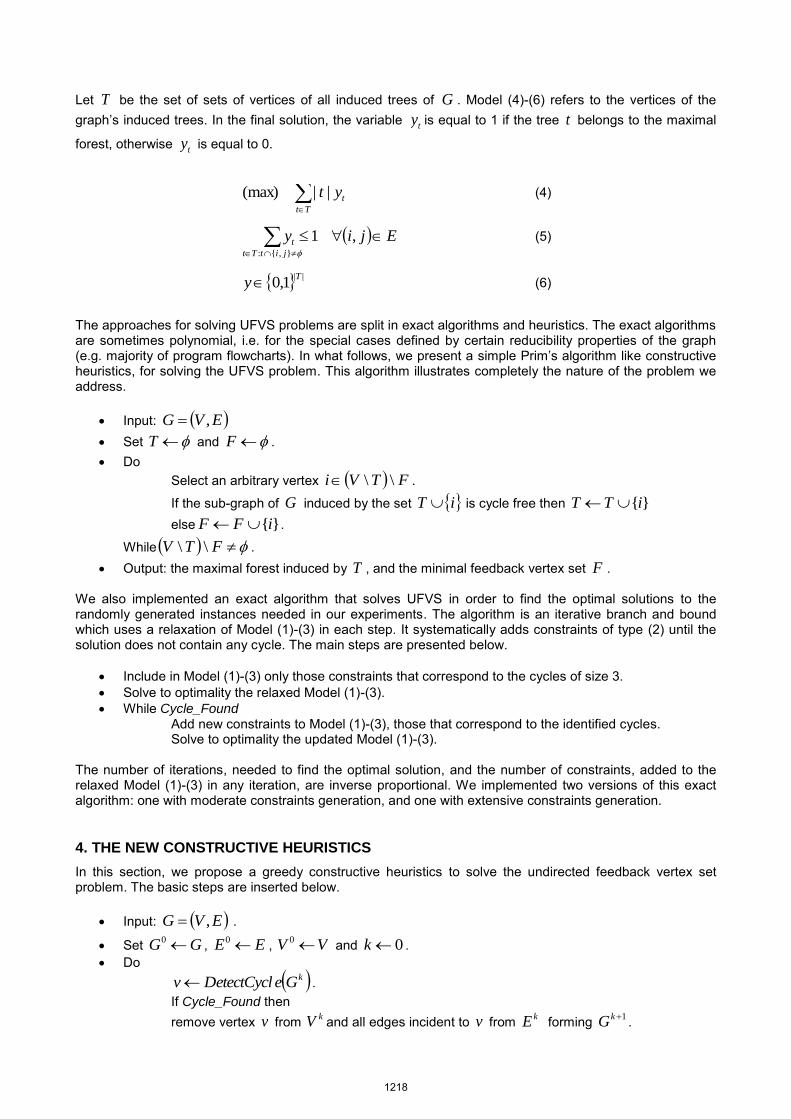
Let T be the set of sets of vertices of all induced trees of G . Model (4)-(6) refers to the vertices of the graph’s induced trees. In the final solution, the variable ty is equal to 1 if the tree t belongs to the maximal

forest, otherwise ty is equal to 0.

Tt

tyt ||(max) (4)

EjiyjitTt

t

,1},{:

(5)

||1,0

Ty (6)

The approaches for solving UFVS problems are split in exact algorithms and heuristics. The exact algorithms are sometimes polynomial, i.e. for the special cases defined by certain reducibility properties of the graph (e.g. majority of program flowcharts). In what follows, we present a simple Prim’s algorithm like constructive heuristics, for solving the UFVS problem. This algorithm illustrates completely the nature of the problem we address.

Input: EVG , Set T and F . Do

Select an arbitrary vertex FTVi \\ .

If the sub-graph of G induced by the set iT is cycle free then }{iTT else }{iFF .

While FTV \\ . Output: the maximal forest induced by T , and the minimal feedback vertex set F .

We also implemented an exact algorithm that solves UFVS in order to find the optimal solutions to the randomly generated instances needed in our experiments. The algorithm is an iterative branch and bound which uses a relaxation of Model (1)-(3) in each step. It systematically adds constraints of type (2) until the solution does not contain any cycle. The main steps are presented below.

Include in Model (1)-(3) only those constraints that correspond to the cycles of size 3. Solve to optimality the relaxed Model (1)-(3). While Cycle_Found

Add new constraints to Model (1)-(3), those that correspond to the identified cycles. Solve to optimality the updated Model (1)-(3).

The number of iterations, needed to find the optimal solution, and the number of constraints, added to the relaxed Model (1)-(3) in any iteration, are inverse proportional. We implemented two versions of this exact algorithm: one with moderate constraints generation, and one with extensive constraints generation.

4. THE NEW CONSTRUCTIVE HEURISTICS

In this section, we propose a greedy constructive heuristics to solve the undirected feedback vertex set problem. The basic steps are inserted below.

Input: EVG , .

Set GG 0 , EE 0 , VV 0 and 0k . Do

kGeDetectCyclv . If Cycle_Found then remove vertex v from kV and all edges incident to v from kE forming 1kG .

1218

1 kk . While Cycle_Found.

Output: the maximal forest kkk EVG , , and the minimal feedback vertex set kVVF \ . The function GeDetectCycl detects a cycle in G , and returns the vertex from the cycle with the largest degree. The same function sets the global variable Cycle-Found to ‘TRUE’ if the graph G contains at least one cycle, or otherwise, to ‘FALSE’. Removing the vertex with the largest degree favors breaking more cycles at once, but also makes the heuristics greedy.

Figure 1: The graph used to describe how the procedure DetectCycle() works

A simple example of a graph and its minimal feedback vertex set is shown in Figure 1. Starting from the graph 000 ,EVG where 5,4,3,2,10 V and 5,4,5,3,4,3,5,2,3,2,5,1,2,10 E , the first detected cycle is 1-2-5. Further, the vertex 5, the vertex with the largest degree in the cycle, is returned by the function DetectCycle(). Then, vertex 5 is removed from the set of vertices together with all edges adjacent to it, i.e. 5,4,5,3,5,2,5,1 . Thus, the graph 111 ,EVG is defined, where 4,3,2,11 V

and 4,3,3,2,2,11 E . This graph is cycle free, hence the maximal forest is 111 ,EVG , and the

minimum feedback vertex set is 5F . The computational complexity of the cycle detection step is 2VO .

Figure 2: The graph used to show a situation when the new heuristic misses to find the exact solution

Running our heuristics for finding the minimum FVS of the graph presented in Figure 2, the following unfortunate situation appears: the detected cycle is 1-2-3-4; the vertex with the largest degree in the cycle is 4; the graph remains with cycles after eliminating 4 and its edges; the new graph after this step is

5,3,5,2,3,2,2,1,7,6,5,3,2,11 G . The next detected cycle is 2-3-5; vertex 2 and its edges are

eliminated; and the final FVS is 4,2F and the final forest is 5,3,7,6,5,3,12 G . In fact, the minimum FVS contains one vertex and can be obtained in the first step, by removing the vertex 3 from the cycle 1-2-3-4.

5. COMPUTATIONAL RESULTS

For our experiments, we implemented the exact algorithm and the new heuristics that solve UFVS problems. We generated randomly 250 instances, and grouped them according to the number of vertices v (20, 30, 40, 50, and 60) and density d (10, 30, 50, 70, and 90).

1219

Table 1: The results obtained by running the exact algorithm

Density # vertices # instances solved exactly

Average time (for instances solved exactly)

% Dev of LB from UB (for instances not solved exactly)

10

20 10 0 N/A 30 10 0 N/A 40 10 0.32 N/A 50 10 75.07 N/A 60 6 1934.50 3.27%

30

20 10 0.09 N/A 30 10 22.89 N/A 40 10 1433.96 N/A 50 0 N/A 8.21% 60 0 N/A 20.78%

50

20 10 0.97 N/A 30 10 135.84 N/A 40 3 6862.80 9.64% 50 0 N/A 9.92% 60 0 N/A 20.00%

70

20 10 2.05 N/A 30 10 442.01 N/A 40 8 4184.96 12.50% 50 1 5888.30 13.58% 60 0 N/A 17.65%

90

20 10 3.44 N/A 30 10 173.19 N/A 40 10 1605.88 N/A 50 7 2934.14 16.67% 60 4 2602.50 16.67%

For each pair of values (v, d) we generated 10 instances as follows: we arranged the edges into an array of

size 2

2 vv ; following the uniform distribution, we randomly generated, d times, an index that refers to a

component of the array. The first index was generated between 1 and 2v , the second index was generated between the first index and 2v , and so on; when we reached the component 2v , we started from the beginning. Table 1 summarizes the computational results obtained by running the exact algorithm. For each group of instances, we reported how many instances out of 10 we solved exactly in less than 7200 seconds; the average time needed for exactly solved instances; and the average deviation of the lower bound from the upper bound in the case of instances that we did not solved exactly. The computational results showed that the exact algorithm best performs when the density of the graph is either very small ( 10d ) or very large ( 90d ). In addition, for middle values of the density ( 30d , 50d , and 70d ), the algorithm has a significant low performance when the number of vertices in the graph increases from 50 to 60. In order to describe the performance of the new heuristics, we summarized our computational results in Table 2. For each group of instances, we reported the average percentage of the deviations of the size of the obtained forest from the size of the optimal forest (or, from the upper bound found for the size of the optimal forest, when we were not able to solve the instance exactly in less than 7200 seconds). In Table 2, d represents the density of the graphs that, together with the number of vertices, characterizes the groups of instances.

1220

Table 2: The results obtained by running the heuristics (the percent of the deviation of the obtained forest size from the optimal solution or from the upper bound when the instance was not solved exactly in 7200s)

# vertices d = 10 d = 30 d = 50 d = 70 d = 90 20 1.62% 3.36% 3.41% 6.15% 9.09% 30 2.39% 6.00% 4.90% 5.63% 10.00% 40 1.64% 5.81% 10.17% 5.00% 3.92% 50 3.43% 12.31% 14.50% 20.00% 8.77% 60 4.38% 21.65% 20.67% 19.61% 10.00%

Similar to the case of the exact algorithm, the experimental results showed a good performance of the new heuristics when the density of the graph was either very small or very large. Also, relatively good performance was noticed for the graphs with middle values of the density and number of vertices up to 50.

6. CONCLUSION AND FUTURE WORK

In this paper, we addressed the feedback vertex set problem, and proposed a new constructive heuristics to solve it. We tested our heuristics on random generated instances of various densities and number of vertices. We described the performance of our exact algorithm by counting the number of instances solved to optimality in a certain time, and the average difference between the lower and upper bounds, when the exact solution was not reached. Further, we reported the computational results as percentage of deviations of the approximate solutions from the exact solutions of the instances or from the upper bound, when we were not able to find the exact solution in reasonable time by the exact algorithm. Our intention is to perform additional experiments in order to compare our heuristics to other constructive heuristics found in literature. Including some randomization steps, we can extend this heuristics to a GRASP procedure and/or a set-covering approach, thus improve its performance. Our intention is also to develop a meta-heuristics based on VNS to solve the FVS problems.

ACKNOWLEDGMENTS

This research was partially supported by the Ministry of Education and Science, Republic of Serbia, Project numbers TR32013 and TR36006.

REFERENCES

Bar-Yehuda, R., Geiger, D., Naor, J. & Roth, R. M. (1994). Approximation algorithms for vertex feedback set problem with applications to constraint satisfaction and Bayesian inference, Proceedings of the Fifth Annual ACM-SIAM Symposium on Discrete Algorithms, Arlington, Virginia, pp. 344-354.

Chen, J., Fomin, F. V., Liu, Y., Lu, S. & Villanger, Y. (2008). Improved algorithms for feedback vertex set problems. Journal of Computer and System Sciences, 74,1188-1198. doi:10.1016/j.jcss.2008.05.002

Chen, H. B., Fu, H. L. & Shih, C. H. (2012) Feedback vertex set on planar graphs. Taiwanese Journal of Mathematics, 16(6) 2077-2082.

Festa, P., Pardalos, P. M. & Resende, M. G. C. (2000). Feedback set problems. In Du, D.-Z. & Pardalos, P. M. (Eds.). Handbook of Combinatorial Optimization, Supplement vol. A, Kluwer Academic Publishers, pp. 209–259.

Fomin, F. V., Gaspers, S., Pyatkin, A. & Razgon, I. (2008) On the minimum feedback vertex set problem: exact and enumeration algorithms. Algorithmica, 52(2) 293–307. doi:10.1007/s00453-007-9152-0

Gaspers, S. & Mnich, M. (2013). Feedback Vertex Sets in Tournaments. Journal of Graph Theory. 72(1) 72-89. doi:10.1002/jgt.21631

Jiang, W., Liu, T. Wang, C. & Xu, K. (2013). Feedback vertex sets on restricted bipartite graphs. Theoretical Computer Science, 507, 41-51. doi:10.1016/j.tcs.2012.12.021

Karp, R. M. (1972). Reducibility among combinatorial problems. In: Complexity of computer computations, Plenum Press, New York, pp. 85-103.

Silberschatz, A., Galvin, P. B. & Gagne, G. (2008). Operating System Concepts (8th ed.), John Wiley & Sons. Inc.

Xiao , M. & Nagamochi , H. (2013). An Improved Exact Algorithm for Undirected Feedback Vertex Set. In: Combinatorial Optimization and Applications, Lecture Notes in Computer Science. 8287, Springer International Publishing, pp 153-164. doi: 10.1007/978-3-319-03780-6_14

1221