operational analysis methods - safety analysis methods signalized intersections: informational guide...

Chapter 7. Operational Analysis Methods

Signalized Intersections: Informational Guide 7-1

CHAPTER 7

OPERATIONAL ANALYSIS METHODS

TABLE OF CONTENTS

7.0 OPERATIONAL ANALYSIS METHODS............................................................................. 7-2 7.1 Operational Performance Measures ......................................................................... 7-5

7.1.1 Automobile Methodology ............................................................................. 7-6 7.1.2 Pedestrian Methodology .............................................................................. 7-9 7.1.3 Bicycle Methodology .................................................................................. 7-10 7.1.4 Multimodal Approach ................................................................................. 7-11

7.2 Traffic Operations Elements ................................................................................... 7-11 7.2.1 Traffic Volume Characteristics ................................................................... 7-11 7.2.2 Intersection Geometry ................................................................................ 7-12 7.2.3 Signal Timing and Hardware Capabilities .................................................. 7-12

7.3 General Considerations Sizing an Intersection ....................................................... 7-13 7.4 Critical Lane Analysis .............................................................................................. 7-14 7.5 HCM Operational Procedure for Signalized Intersections ...................................... 7-17 7.6 Arterial and Network Signal Timing Models ............................................................ 7-18

7.6.1 Introduction ................................................................................................ 7-18 7.6.2 Developing a Macroscopic Simulation Model ............................................ 7-18

7.7 Microscopic Simulation Models ............................................................................... 7-19 7.7.1 Introduction ................................................................................................ 7-19 7.7.2 Developing a Microsimulation Model ......................................................... 7-19

7.8 Operational Performance Model Selection ............................................................. 7-20

LIST OF EXHIBITS 7-1 Still reproduction of a graphic from an animated traffic operations model ......................... 7-3 7-2 Overview of intersection traffic analysis models ................................................................. 7-4 7-3 Typical lane groups for analysis ......................................................................................... 7-6 7-4 Automobile LOS thresholds at signalized intersections...................................................... 7-8 7-5 Effect of flow rate and detection design on max-out probability ......................................... 7-9 7-6 Evaluation of circulation area based on pedestrian space ................................................. 7-9 7-7 LOS criteria for pedestrian and bicycle modes ................................................................. 7-10 7-8 Planning-level guidelines for sizing an intersection .......................................................... 7-14 7-9 Graphical summary of the quick estimation method ......................................................... 7-15 7-10 V/C ratio threshold descriptions for the quick estimation method .................................... 7-16 7-11 Criteria for selecting a traffic analysis tool category ......................................................... 7-21



7.0 OPERATIONAL ANALYSIS METHODS

Chapter 6 described tools that can be used to assess safety performance at a signalized intersection. Evaluating a candidate treatment also usually requires assessing its performance from the perspective of traffic operations. This chapter will focus on measures for assessing operational performance and computational procedures used to determine specific values for those measures.

The relationships between safety performance and operational performance are difficult to define in general terms. Some intersection treatments that would improve safety might also improve operational performance, but others might diminish operational performance. Furthermore, the nature of safety and operational measures makes them difficult to combine in a way that would represent both perspectives.

Operational performance measures tend to be fewer in number and more easily related to site-specific conditions than are safety performance measures. The computations themselves are more amenable to deterministic models, and a wide variety of such models, mostly software-based, are available. Selection of a model for a specific purpose is generally based on the tradeoff between the difficulty of applying the model and the required degree of accuracy and confidence in the results. The degree of application difficulty is reflected in the required amount of site-specific data as well as the level of personnel time and training needed to apply the model and to interpret the results.

Recent user interface enhancements in the more advanced traffic model software products have made the products much easier to apply. Most can generate animated graphics displays depicting the movement of individual vehicles and pedestrians in an intersection (see Exhibit 7-1) and some allow for three-dimensional rendering. These enhancements have caused an increasing trend toward the use and acceptance of advanced traffic modeling techniques.

While the range of operational performance models is more or less continuous, it will be categorized into the following analysis levels for purposes of this discussion:

• Rules of thumb for intersection sizing.

• Critical lane analysis.

• The HCM 2010 operational analysis procedure.(2)

• Arterial signal timing design and evaluation models.

• Microscopic simulation models.

These levels are listed in order of complexity and application difficulty, from least to greatest. Each analysis level will be discussed separately.

The process for evaluating the operational performance of an intersection remains unchanged regardless of the analysis level and the issues at hand. The analysis should begin at the highest level and should continue to the next level of detail until the key operations-related issues and concerns have been addressed in sufficient detail. Additional guidance for each level above can be found in the FHWA Traffic Analysis Tools Program website at http://ops.fhwa.dot.gov/trafficanalysistools/.

http://ops.fhwa.dot.gov/trafficanalysistools/



Exhibit 7-1. Still reproduction of a graphic from an animated traffic operations model.



Exhibit 7-2. Overview of intersection traffic analysis models.

The ability to measure, evaluate, and forecast traffic operations is a fundamental element of effectively diagnosing problems and selecting appropriate treatments for signalized intersections. A traffic operations analysis should describe how well an intersection accommodates demand for all user groups. Traffic operations analysis can be used at a high level to size a facility and at a refined level to develop signal timing plans. This section describes key elements of signalized intersection operations and provides guidance for evaluating results.

In all analysis methods, especially those that involve modeling, it is important that any tools used are calibrated and validated for real-life field conditions to ensure credible analysis results. Data collected include entering traffic volume, turning movements, queue lengths, vehicle speed, and lane capacity. Modifications to the software tools may be necessary to accurately reflect field conditions. It is necessary to document all calibration adjustments to support credibility.



7.1 OPERATIONAL PERFORMANCE MEASURES A signalized intersection’s performance is described by the use of one or more quantitative

measures that characterize some aspects of the service provided to specific road user groups. The HCM 2010 introduces four road user groups: automobile, pedestrian, bicycle, and transit. In order to encourage users to consider all travelers on a facility when they perform analyses and make decisions, the HCM 2010 integrates material on automobile and non-automobile modes.

Generally, three methodologies are used to evaluate the performance measures of signalized intersection operations. They are referred to as the automobile methodology, the pedestrian methodology, and the bicycle methodology. Each methodology addresses one possible travel mode through the intersection. A complete evaluation of intersection operation includes the separate examination of performance for all relevant travel modes. The performance measures associated with each travel mode are as follows:

a) Automobile mode

• Capacity and volume-to-capacity ratio.

• Delay and Level of Service (LOS).

• The back-of-queue and queue storage ratio.

• Probability of phase termination by max out or force-off.

b) Pedestrian mode

• Corner and crosswalk circulation area.

• Pedestrian delay.

• Pedestrian LOS score.

c) Bicycle mode

• Bicycle delay.

• Bicycle LOS score.

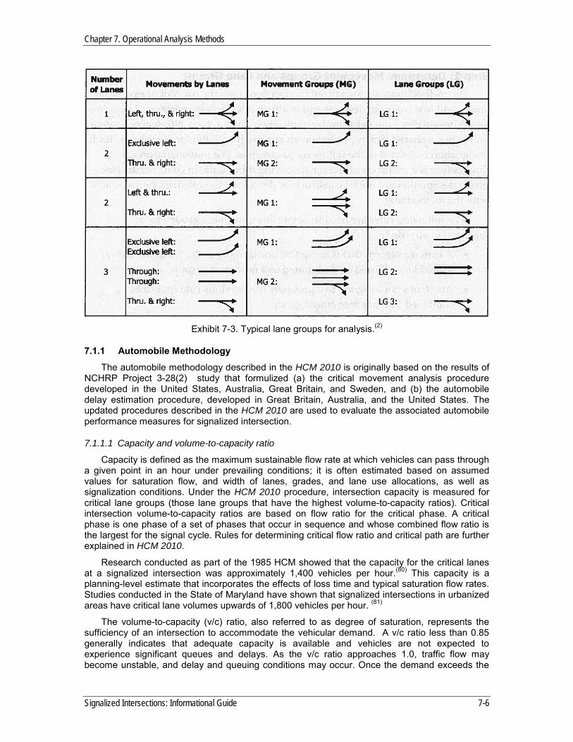
The HCM 2010 evaluates the intersection operation by the concept of movement groups and lane groups.(2) A separate movement group is established for (a) each turn movement with one or more exclusive turn lanes with no shared movements, and (b) the through movement inclusive of any turn movements that share a lane.

The movement group and lane group designations are very similar in meaning. In fact, their differences emerge only when a shared lane (such as a through lane that is also serving right turns) is present on an approach with two or more lanes. (2) Thus, any shared lane is considered as a separate lane group, while an exclusive turn lane or lanes should be designated as another separate lane group. Similar to movement group definition, any lanes that are not exclusive turn lanes or shared lanes are combined into one lane group. These rules for movement group and lane group result in designation of different group possibilities for an intersection approach. Exhibit 7-3 presents some common movement groups and lane groups.(2)



Exhibit 7-3. Typical lane groups for analysis.(2)

7.1.1 Automobile Methodology

The automobile methodology described in the HCM 2010 is originally based on the results of NCHRP Project 3-28(2) study that formulized (a) the critical movement analysis procedure developed in the United States, Australia, Great Britain, and Sweden, and (b) the automobile delay estimation procedure, developed in Great Britain, Australia, and the United States. The updated procedures described in the HCM 2010 are used to evaluate the associated automobile performance measures for signalized intersection.

7.1.1.1 Capacity and volume-to-capacity ratio

Capacity is defined as the maximum sustainable flow rate at which vehicles can pass through a given point in an hour under prevailing conditions; it is often estimated based on assumed values for saturation flow, and width of lanes, grades, and lane use allocations, as well as signalization conditions. Under the HCM 2010 procedure, intersection capacity is measured for critical lane groups (those lane groups that have the highest volume-to-capacity ratios). Critical intersection volume-to-capacity ratios are based on flow ratio for the critical phase. A critical phase is one phase of a set of phases that occur in sequence and whose combined flow ratio is the largest for the signal cycle. Rules for determining critical flow ratio and critical path are further explained in HCM 2010.

Research conducted as part of the 1985 HCM showed that the capacity for the critical lanes at a signalized intersection was approximately 1,400 vehicles per hour.(80) This capacity is a planning-level estimate that incorporates the effects of loss time and typical saturation flow rates. Studies conducted in the State of Maryland have shown that signalized intersections in urbanized areas have critical lane volumes upwards of 1,800 vehicles per hour. (81)

The volume-to-capacity (v/c) ratio, also referred to as degree of saturation, represents the sufficiency of an intersection to accommodate the vehicular demand. A v/c ratio less than 0.85 generally indicates that adequate capacity is available and vehicles are not expected to experience significant queues and delays. As the v/c ratio approaches 1.0, traffic flow may become unstable, and delay and queuing conditions may occur. Once the demand exceeds the



capacity (a v/c ratio greater than 1.0), traffic flow is unstable and excessive delay and queuing is expected. Aside from the excessive demand, there are other factors that may contribute to cycle failure as well (e.g., influence of pedestrians, poor signal timing, incidents, etc.). Under these conditions, vehicles may require more than one signal cycle to pass through the intersection (known as a cycle failure). For design purposes, a v/c ratio between 0.85 and 0.95 generally is used for the peak hour of the horizon year (generally 20 years out). Over-designing an intersection should be avoided due to negative impacts to all users associated with wider street crossings, the potential for speeding, land use impacts, and cost.

Delay Delay is defined in the HCM 2010 as “the additional travel time experienced by a driver,

passenger, bicyclist, or pedestrian beyond that is required to travel at the desired speed.”(2) The signalized intersection chapter (Chapter 18) of the HCM 2010 provides equations for calculating control delay, the delay a motorist experiences that is attributable to the presence of the traffic signal and conflicting traffic. This includes time spent decelerating, in the queue, and accelerating. Expectation of delay at a signalized intersection is different than at an unsignalized intersection.

The control delay equation comprises three elements: uniform delay, incremental delay, and initial queue delay. The primary factors that affect uniform delay are lane group volume, lane group capacity, cycle length, and effective green time. Two factors that account for incremental delay are (a) the effect of random and cycle-by-cycle fluctuations in demand that occasionally exceed capacity, and (b) a sustained oversaturation during the analysis period, when the aggregate demand exceeds the aggregate capacity. The third component of the control delay illustrates the delay due to an initial queue, as a result of unmet demand in the previous time period.

The Back-of-queue and Queue Storage Ratio Practitioners should evaluate vehicle queuing, an important performance measure, as part of

all signalized intersections analyses. Vehicle queue estimates help determine the amount of storage required for turn lanes and whether spillover occurs at upstream facilities (driveways, unsignalized intersections, signalized intersections, etc.). Queues that extend upstream from an intersection can spill back into and block upstream intersections, causing side streets to begin to queue back. The back-of-queue is the maximum backward extent of queued vehicles during a typical cycle. This back-of-queue length depends on the arrival pattern of vehicles and the number of vehicles that do not clear the intersection during the previous cycle.(2) Approaches that experience extensive queues also may experience an over-representation of rear-end collisions. Vehicle queues for design purposes are typically estimated based on the 95th percentile queue that is expected during the design period. This is the length at which 95 percent of lane queues are less than in a given study period.

The queue storage ratio represents the proportion of the available queue storage distance that is occupied at the point in the cycle when the back-of-queue position is reached.(2) If this ratio exceeds 1.0, then the storage space will overflow and queued vehicles may block other vehicles from moving forward.

Volume 3 of the HCM 2010 provides procedures for calculating back-of-queue length and the queue storage ratio. In addition, all known simulation models provide ways of obtaining queue estimates.

Level of Service (LOS) Level of Service (LOS) is a grading-scale based descriptor that attempts to relate relative

operational quality (based on certain measures of effectiveness) to that of driver perception in a simple fashion. Control delay is used as the basis for determining LOS for an intersection or a single approach. Delay thresholds for the various LOS are given in Exhibit 7-4.



Typically LOS is reported on an A through F scale, with Level A being the best LOS and Level F being the worst. While the A through F scale seems fairly straightforward, the quantifiable measures of effectiveness (MOEs) used to derive the “grading scale” are derived from empirical data.

For signalized intersections, control delay (in seconds) is the MOE for the LOS scale (note that the grade thresholds for signalized intersections are different than for stop-controlled intersections). However, there are other MOEs that are important in characterizing the operations of signalized intersections, including v/c ratio and intersection utilization. Furthermore, while it is common for weighted averages to be used in describing overall intersection operation, it is often the case where one or more specific movements, lane groups, or approaches may be operating poorly, but be masked by the overall average. Also, when intersections are operating at capacity (i.e., LOS F) and beyond, only close analysis of the various MOEs will allow for distinctions to be made among different alternatives. Finally, it should be noted that safety is not reflected or implied in LOS.

Exhibit 7-4. Automobile LOS thresholds at signalized intersections.(2)

Control Delay per Vehicle (seconds per vehicle)

LOS by V/C Ratio ≤1 >1

≤ 10 A F > 10-20 B F > 20-35 C F > 35-55 D F > 55-80 E F

> 80 F F

LOS has historically been given high emphasis by practitioners due to its relative ease of

explanation, but it is a crude measure at best. The language of LOS (A-F scale) is easily understood, regardless of the background MOEs used or their accuracy in actually determining the operation of the intersection.

Probability of Phase Termination by Max-out or Force-off For actuated and semi-actuated operation, the maximum green time is the maximum limit to

which the green time can be extended for a phase in the presence of a call from a conflicting phase. The maximum green time begins when a call is placed on a conflicting phase. The phase is allowed to "max-out" if the maximum green time is reached even if actuations have been received that would typically extend the phase. However, the safety benefit of green extension can be negated if the phase is extended to its maximum duration (i.e., maximum-green setting). The probability of termination by “max-out” is dependent on flow rate in the subject phase and the “maximum allowable headway.” Exhibit 7-5 illustrates the relationship between max-out probability, maximum allowable headway, maximum green, and flow rate for actuated and semi-actuated operation. For coordinated operation, the main street phase will receive its entire split time (effectively a force-off) regardless of calls on conflicting phases.



Exhibit 7-5. Effect of flow rate and detection design on max-out probability.

Source: Bonneson, J. et al, Intelligent Detection-Control System for Rural Signalized Intersections, FHWA/TX-03/4022-2, 2002.

7.1.2 Pedestrian Methodology

This section describes the methodology for evaluating the performance of a signalized intersection in terms of its service to pedestrians.

Corner and Crosswalk Circulation Area The corner and crosswalk circulation area are used to evaluate the circulation area provided

to pedestrians while they are waiting at the corner or crossing the crosswalk, respectively. Exhibit 7-6 can be used to evaluate intersection performance from a circulation-area prospective in terms of space available to the average pedestrian.(2)

Exhibit 7-6. Evaluation of circulation area based on pedestrian space.(2)

Pedestrian Space (ft2 per pedestrian)

Description

>60 Ability to move in desired path, no need to alter movements > 40-60 Occasional need to adjust path to avoid conflicts > 24-40 Frequent need to adjust path to avoid conflicts > 15-24 Speed and ability to pass slower pedestrian restricted > 8-15 Speed restricted, very limited ability to pass slower pedestrian

≤ 8 Speed severely restricted, frequent contact with other users

The critical parameter for the analysis of circulation area at the street corner and crosswalk is the product of available time and space with pedestrian demand, which combines the physical design constrains (i.e., available space) and signal operation (i.e., available time). This parameter is referred to as the “time-space” available for pedestrian circulation.(2) Circulation time-space and pedestrian circulation area are estimated based on intersection and pedestrian signal phasing settings, pedestrian flow rates in different directions, and physical characteristics of the sidewalks. Chapter 18 of the HCM 2010 provides the detailed procedure for calculating street corner and crosswalk circulation area.



Pedestrian Delay In the HCM 2010 (Chapter 18), pedestrian delay at a signalized intersection while crossing

the major street is determined based on effective walk time and cycle length. The delay computed in this step can be used to make judgments about pedestrian compliance. Research indicates that pedestrians become impatient when they experienced delay in excess of 30 seconds per pedestrian. In contrast, it is reported that pedestrians are very likely to comply with signal indicators if their expected delay is less than 10 seconds per pedestrian.(2)

Pedestrian LOS Score Historically, the HCM has used a single performance measure as the basis for defining LOS.

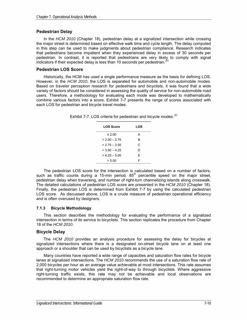
However, in the HCM 2010, the LOS is separated for automobile and non-automobile modes. Based on traveler perception research for pedestrians and bicyclists, it was found that a wide variety of factors should be considered in assessing the quality of service for non-automobile road users. Therefore, a methodology for evaluating each mode was developed to mathematically combine various factors into a score. Exhibit 7-7 presents the range of scores associated with each LOS for pedestrian and bicycle travel modes.

Exhibit 7-7. LOS criteria for pedestrian and bicycle modes.(2)

LOS Score LOS

≤ 2.00 A > 2.00 – 2.75 B > 2.75 – 3.50 C > 3.50 – 4.25 D > 4.25 – 5.00 E

> 5.00 F

The pedestrian LOS score for the intersection is calculated based on a number of factors, such as traffic counts during a 15-min period, 85th percentile speed on the major street, pedestrian delay when traversing, and number of right-turn channelizing islands along crosswalk. The detailed calculations of pedestrian LOS score are presented in the HCM 2010 (Chapter 18). Finally, the pedestrian LOS is determined from Exhibit 7-7 by using the calculated pedestrian LOS score. As discussed above, LOS is a crude measure of pedestrian operational efficiency and is often overused by designers.

7.1.3 Bicycle Methodology

This section describes the methodology for evaluating the performance of a signalized intersection in terms of its service to bicyclists. This section replicates the procedure from Chapter 18 of the HCM 2010.

Bicycle Delay The HCM 2010 provides an analysis procedure for assessing the delay for bicycles at

signalized intersections where there is a designated on-street bicycle lane on at least one approach or a shoulder that can be used by bicyclists as a bicycle lane.

Many countries have reported a wide range of capacities and saturation flow rates for bicycle lanes at signalized intersections. The HCM 2010 recommends the use of a saturation flow rate of 2,000 bicycles per hour as an average value achievable at most intersections. This rate assumes that right-turning motor vehicles yield the right-of-way to through bicyclists. Where aggressive right-turning traffic exists, this rate may not be achievable and local observations are recommended to determine an appropriate saturation flow rate.



Using the default saturation flow rate of 2,000 bicycles per hour, the capacity of the bicycle lane and control delay at a signalized intersection can be computed, based on effective green time for the bicycle lane, and cycle length.

At most signalized intersections, the only delay to bicycles is caused by the signal itself because bicycles have right-of-way over turning motor vehicles. Where bicycles are forced to weave with motor vehicle traffic or where bicycle right-of-way is disrupted due to turning traffic, additional delay may be incurred. Bicyclists tend to have about the same tolerance for delay as pedestrians.

Bicycle LOS Score Following the same methodology as pedestrian mode, bicycle LOS score is first calculated

based on physical characteristics of the intersection, traffic flow rate, and the proportion of on-street occupied parking. The detailed calculations of bicycle LOS score are presented in the HCM 2010 (Chapter 18). Finally, the bicycle LOS is determined from Exhibit 7-7 by using the calculated bicycle LOS score. As discussed above, LOS is a crude measure of pedestrian operational efficiency and is often overused by designers.

7.1.4 Multimodal Approach

In the HCM 2010, there are no stand-alone analyses for pedestrians, bicyclists, and transit users. Instead, the HCM encourages performing multimodal analysis of non-automobile modes on a specific facility of urban streets, such as a signalized intersection, in addition to automobile analysis. The Transit Capacity and Quality of Service Manual (TCQSM), recognized as the companion of HCM 2010, extensively covers the analysis of the transit mode. Therefore, the HCM 2010 now addresses the transit mode only with respect to multimodal analysis of urban streets.(2)

7.2 TRAFFIC OPERATIONS ELEMENTS The following sections will describe signalized intersection operations as a function of the following three elements and discuss their effects on operations.

1. Traffic volume characteristics.

2. Roadway geometry.

3. Signal timing and hardware capabilities.

7.2.1 Traffic Volume Characteristics

The traffic characteristics used in an analysis can play a critical role in determining intersection treatments. Over-conservative judgment may result in economic inefficiencies due to the construction of unnecessary treatments or an oversized intersection, while the failure to account for certain conditions (such as a peak recreational season) may result in facilities that are inadequate and experience failing conditions during certain periods of the year.

An important element of developing an appropriate traffic profile is distinguishing between traffic demand and traffic volume. For an intersection, traffic demand represents the arrival pattern of vehicles, while traffic volume is generally measured as the number of vehicles that pass through the intersection over a specific period of time. In the case of overcapacity or constrained situations, the traffic volume typically does not reflect the true demand on an intersection because vehicles are queued upstream. In these cases, the user should develop a demand profile by measuring vehicle arrivals upstream of the overcapacity or constrained approach. The difference between arrivals and departures represents the vehicle demand that does not get served by the traffic signal. This volume should be accounted for in the traffic operations analysis.

Traffic volume at an intersection may also be less than the traffic demand due to an overcapacity condition at an upstream or downstream signal. If the constraint is upstream, traffic



volumes would be metered at that location and “starve” the demand at the subject intersection; if the constraint is downstream, traffic could spill back to the subject intersection and impede traffic flow. These effects are often best accounted for using a microsimulation analysis tool.

7.2.2 Intersection Geometry

The geometric features of an intersection influence the service volume or amount of traffic an intersection can process. A key measure used to establish the supply of an intersection is saturation flow, which is similar to capacity in that it represents the number of vehicles that traverse a point per hour. However, saturation flow is reported assuming the traffic signal is green the entire hour. By knowing the saturation flow and signal timing for an intersection, one can calculate the capacity (capacity = saturation flow times the ratio of green time to cycle length). Saturation headway is determined by measuring the average time headway between vehicles that discharge from a standing queue at the start of green, beginning with the fourth vehicle.(2) Saturation headway is expressed in time (seconds) per vehicle.

Saturation flow rate is simply determined by dividing the average saturation headway into the number of seconds in an hour (3,600) to yield units of vehicles per hour. The HCM 2010 uses a default ideal saturation flow rate of 1,900 vehicles per hour. Ideal saturation flow assumes the following:

• 12-ft wide travel lanes.

• Through movements only.

• Even lane utilization,

• Level grades.

• No curbside impedances

• No pedestrians/bicyclists.

• No central business district influences.

The HCM 2010 provides adjustment factors for non-ideal conditions to estimate the prevailing saturation flow rate. Saturation flow rate can vary in time and location and has been observed to range between 1,500 and 2,000 passenger cars per hour per lane.(2) Given the variation that exists in saturation flow rates, local data should be collected where possible to improve the accuracy of the analysis.

Practitioners should evaluate existing or planned intersection geometry to determine features that may impact operations and that require special consideration.

7.2.3 Signal Timing and Hardware Capabilities

The signal timing of an intersection also plays an important role in its operational performance. Key factors include:

• Effective green time. Effective green time represents the amount of usable time available to serve vehicular movements during a phase of a cycle. It is equal to the displayed green time minus startup lost time. The effective green time for each phase is generally determined based on the proportion of volume in the critical lane for that phase relative to the total critical volume of the intersection. If not enough green time is provided, vehicle queues will not be able to clear the intersection, and cycle failures will occur. If too much green time is provided, portions of the cycle will be unused, resulting in inefficient operations and frustration for drivers on the adjacent approaches.



• Change and clearance interval. The change and clearance interval represents the amount of time needed for vehicles to safely clear the intersection. It includes the yellow change and red clearance intervals and is primarily set based on the speed of approaching vehicles and the width of the intersection. The effect of the change and clearance interval on capacity is dependent upon the lost time.

• Lost time. Lost time represents the unused portion of a vehicle phase. Lost time occurs twice during a phase: at the beginning when vehicles are accelerating from a stopped position, and at the end when vehicles decelerate in anticipation of the red indication. Longer lost times reduce the amount of effective green time available and thus reduce the capacity of the intersection. Wide intersections and intersections with skewed approaches or unusual geometrics typically experience greater lost times than conventional intersections.

• Cycle length. Cycle length determines how frequently during the hour each movement is served. It is a direct input, in the case of pre-timed or coordinated signal systems running on a common cycle length, or an output of vehicle actuations, minimum and maximum green settings, and clearance intervals. Cycle lengths that are too short do not provide adequate green time for all phases and result in cycle failures. Longer cycle lengths can result in increased delay and queues for all users, and may result in disobedience of the traffic signal and other aggressive driving behavior.

• Phasing. The phasing plan is based on the treatment of each left turn (protected, permitted, or protected-permitted). The number of phases at a signalized intersection, which is directly correlated with its treatment of left turns, impacts the operating capacity of the intersection as it affects effective green time for each movement.

• Signal Technology. Technology can play a significant role in the operating capacity of a signalized intersection. A pre-timed signal, which provides a fixed amount of green time to each intersection approach independent of actual traffic demand, is the simplest form of operation. Actuated signals rely on vehicle detection technology and generally operate more efficiently by extending signal phases when continuous demand is present and skipping phases that would not be servicing any vehicles. The most advanced signal technology, called adaptive signal control, uses sensors to read current traffic conditions and modify signal timings based on real-time information.

• Progression. Progression is the movement of vehicle platoons from one signalized intersection to the next. A well-progressed or well-coordinated system moves platoons of vehicles so that they arrive during the green phase of the downstream intersection. When this occurs, fewer vehicles arrive on red, and vehicle delays, queues, and stops are minimized. A poorly coordinated system moves platoons such that vehicles arrive on red, which increases the delay and queues for those movements beyond what would be experienced if random arrivals occurred.

• Detector Technology. Use of detector features and settings can impact operations positively or negatively. Employing features such as delay, lock, or switch can improve service to waiting or approaching vehicles and streamline intersection operations. Factors such as volumes, phasing, geometry, and driver characteristics (aggressive or passive) will help influence if and how detector settings are used, and how the controller receives those inputs.

7.3 GENERAL CONSIDERATIONS FOR SIZING AN INTERSECTION

This first level of analysis does not use formal models or procedures; instead, it relies on past experience and rules of thumb to offer a very coarse approximation. In spite of its obvious limitations, this approach can be used to size an intersection and determine appropriate lane configurations. Guidelines for determining intersection geometry at the planning level are shown in Exhibit 7-8.



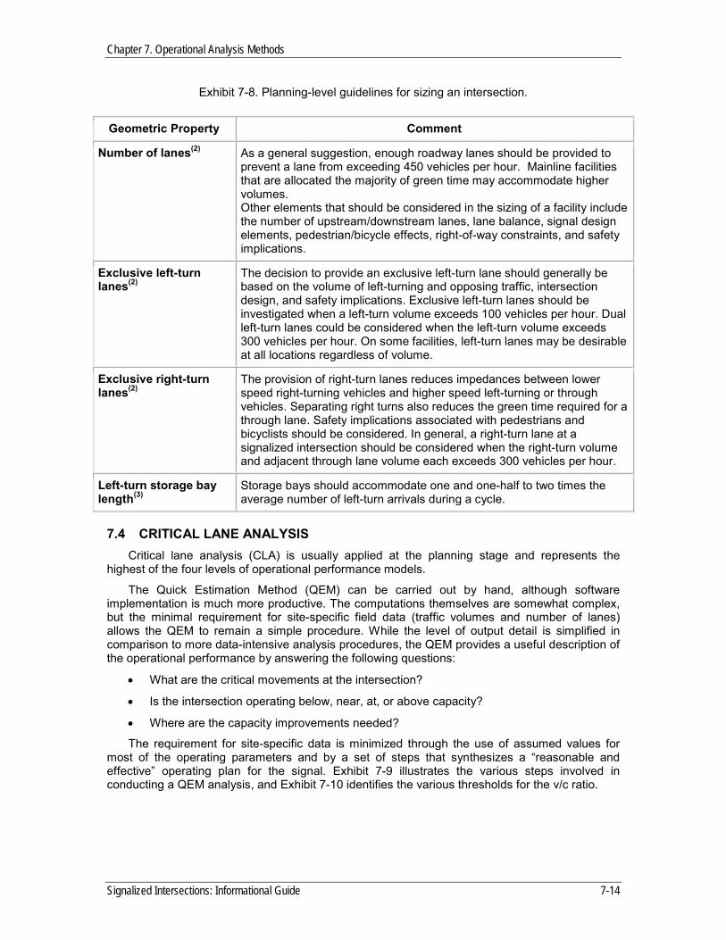
Exhibit 7-8. Planning-level guidelines for sizing an intersection.

Geometric Property Comment

Number of lanes(2) As a general suggestion, enough roadway lanes should be provided to prevent a lane from exceeding 450 vehicles per hour. Mainline facilities that are allocated the majority of green time may accommodate higher volumes. Other elements that should be considered in the sizing of a facility include the number of upstream/downstream lanes, lane balance, signal design elements, pedestrian/bicycle effects, right-of-way constraints, and safety implications.

Exclusive left-turn lanes(2)

The decision to provide an exclusive left-turn lane should generally be based on the volume of left-turning and opposing traffic, intersection design, and safety implications. Exclusive left-turn lanes should be investigated when a left-turn volume exceeds 100 vehicles per hour. Dual left-turn lanes could be considered when the left-turn volume exceeds 300 vehicles per hour. On some facilities, left-turn lanes may be desirable at all locations regardless of volume.

Exclusive right-turn lanes(2)

The provision of right-turn lanes reduces impedances between lower speed right-turning vehicles and higher speed left-turning or through vehicles. Separating right turns also reduces the green time required for a through lane. Safety implications associated with pedestrians and bicyclists should be considered. In general, a right-turn lane at a signalized intersection should be considered when the right-turn volume and adjacent through lane volume each exceeds 300 vehicles per hour.

Left-turn storage bay length(3)

Storage bays should accommodate one and one-half to two times the average number of left-turn arrivals during a cycle.

7.4 CRITICAL LANE ANALYSIS Critical lane analysis (CLA) is usually applied at the planning stage and represents the

highest of the four levels of operational performance models.

The Quick Estimation Method (QEM) can be carried out by hand, although software implementation is much more productive. The computations themselves are somewhat complex, but the minimal requirement for site-specific field data (traffic volumes and number of lanes) allows the QEM to remain a simple procedure. While the level of output detail is simplified in comparison to more data-intensive analysis procedures, the QEM provides a useful description of the operational performance by answering the following questions:

• What are the critical movements at the intersection?

• Is the intersection operating below, near, at, or above capacity?

• Where are the capacity improvements needed?

The requirement for site-specific data is minimized through the use of assumed values for most of the operating parameters and by a set of steps that synthesizes a “reasonable and effective” operating plan for the signal. Exhibit 7-9 illustrates the various steps involved in conducting a QEM analysis, and Exhibit 7-10 identifies the various thresholds for the v/c ratio.



Exhibit 7-9. Graphical summary of the quick estimation method.

Step 1 – Identify movements to be served and assign hourly traffic volumes per lane. This is the only site-specific data that must be provided. The hourly traffic volumes are usually adjusted to represent the peak 15-minute period. The number of lanes must be known to compute the hourly volumes per lane.

Step 2 – Arrange the movements into the desired signal phasing plan. The phasing plan is based on the treatment of each left turn (protected, permitted, etc.). The actual left-turn treatment may be used, if known. Otherwise, the likelihood of needing left-turn protection on each approach will be established from the left-turn volume and the opposing through traffic volume.

Step 3 – Determine the critical volume per lane that must be accommodated on each phase. Each phase typically accommodates two non-conflicting movements. This step determines which movements are critical. The critical lane volume determines the amount of time that must be assigned to the phase on each signal cycle.

Step 4 – Sum the critical phase volumes to determine the overall critical volume that must be accommodated by the intersection. This is a simple mathematical step that produces an estimate of how much traffic the intersection needs to accommodate.

Step 5 – Determine the maximum critical volume that the intersection can accommodate. This represents the overall intersection capacity.

Step 6 – Determine the critical v/c ratio, which is computed by dividing the overall critical volume by the overall intersection capacity, after adjusting the intersection capacity to account for time lost due to starting and stopping traffic on each cycle. The lost time will be a function of the cycle length and the number of protected left turns.

Step 7 – Determine the intersection status from the critical volume-to-capacity ratio. The status thresholds are given in Exhibit 7-10.



Exhibit 7-10. V/C ratio threshold descriptions for the quick estimation method.(2)

Critical Volume-to-Capacity Ratio Assessment

< 0.85 Intersection is operating under capacity. Excessive delays are not experienced.

0.85-0.95 Intersection is operating near its capacity. Higher delays may be expected, but continuously increasing queues should not occur.

0.95-1.0 Unstable flow results in a wide range of delay. Intersection improvements will be required soon to avoid excessive delays.

> 1.0 The demand exceeds the available capacity of the intersection. Excessive delays and queuing are anticipated.

Understanding the critical movements and critical volumes of a signalized intersection is a fundamental element of any capacity analysis. A CLA should be performed for all intersections considered for capacity improvement. The usefulness and effectiveness of this step should not be overlooked, even for cases where more detailed levels of analysis are required. The CLA procedure gives a quick assessment of the overall sufficiency of an intersection. For this reason, it is useful as a screening tool for quickly evaluating the feasibility of a capacity improvement and discarding those that are clearly not viable.

Some limitations of CLA procedures in general, and the QEM in particular:

• No provision exists for the situation in which the timing requirements for a concurrent pedestrian phase (such as for crossing a wide street) exceed the timing requirements for the parallel vehicular phase. As a result, the CLA procedure may underestimate the green time requirements for a particular phase.

• A fixed value is assumed for the overall intersection capacity per lane. Adjustment factors are not provided to account for differing conditions among various sites, and there is no provision for the use of field data to override the fixed assumption.

• Complex phasing schemes such as lagging left-turn phases, right-turn overlap with a left-turn movement, exclusive pedestrian phases, leading/lagging pedestrian intervals, etc., are not considered. Significant operational and/or safety benefits can sometimes be achieved by the use of complex phasing.

• Lost time is not directly accounted for in the CLA procedures. Therefore, the effect of longer change and clearance intervals cannot be directly accommodated with this procedure.

• The synthesized operating plan for the signal does not take minimum green times into account, and therefore may not be readily implemented as a part of an intersection design. The HCM specifically warns against the use of the QEM for signal timing design.

• Performance measures (e.g., control delay, LOS, and back of queue) are not provided.

For these reasons, it will be often necessary to examine the intersection using a more detailed level of operational performance modeling.



7.5 HCM OPERATIONAL PROCEDURE FOR SIGNALIZED INTERSECTIONS For many applications, performance measures such as vehicle delay, LOS, and queues are

desired. These measures are not reported by the CLA procedures, but are provided by macroscopic-level procedures such as the HCM operational analysis methodology for signalized intersections. This procedure is represented as the second analysis level in Exhibit 7-2 Macroscopic-level analyses provide results over multiple cycle lengths based on hourly vehicle demand and service rates. HCM analyses are commonly performed for 15-minute periods to accommodate the heaviest part of the peak hour.

The HCM analysis procedures provide estimates of saturation flow, capacity, delay, LOS, and back of queue by lane group for each approach. Exclusive turn lanes are considered as separate lane groups. Lanes with shared movements are considered a single lane group. Lane group results can be aggregated to estimate average control delay per vehicle at the intersection level.

The increased output detail compared to the CLA procedure is obtained at the expense of additional input data requirements. A complete description of intersection geometrics and operating parameters must be provided. Several factors that influence the saturation flow rates (e.g., lane width, grade, parking, pedestrians) must be specified. A complete signal operating plan, including phasing, cycle length, and green times, must be developed externally. As indicated in Exhibit 7-2, an initial signal operating plan may be obtained from the QEM, or a more detailed and implementable plan may be established using a signal timing model that represents the next level of analysis. Existing signal timing may also be obtained from the field.

In addition to the signalized intersection procedure, the HCM also includes procedures to estimate the LOS for bicyclists, pedestrians, and transit users at signalized intersections. These have been discussed previously in this chapter.

The HCM 2010 provides a more detailed analysis procedure than previous editions as it now has improved methods for calculating delays and queues as well as for analyzing intersections with actuated signals.

Known limitations of the HCM analysis procedures for signalized intersections exist under the following conditions:

• Available software products that perform HCM analyses generally do not accommodate intersections with more than four approaches.

• The analysis may not be appropriate for alternative intersection designs.

• The effect of queues that exceed the available storage bay length is not treated in sufficient detail, nor is the backup of queues that block a stop line during a portion of the green time.

• Driveways located within the influence area of signalized intersections are not recognized.

• The analysis does not explicitly account for travel lanes added just upstream or dropped just downstream of the intersection.

• The effect of arterial progression in coordinated systems is recognized, but only in terms of a coarse approximation.

• Heterogeneous effects on individual lanes within multilane lane groups (e.g., downstream taper, freeway on-ramp, driveways) are not recognized.

If any of these conditions exist, it may be necessary to proceed to the next level of analysis.



7.6 ARTERIAL AND NETWORK SIGNAL TIMING MODELS 7.6.1 Introduction

Arterial and network signal timing models are also macroscopic in nature. They do, however, deal with a higher level of detail and are more oriented to operational design than the HCM. Most of the macroscopic simulation models for signalized intersections are designed to develop optimum signal timing along an arterial. These models are usually used to improve progression between intersections. The effect of traffic progression between intersections is treated explicitly, either as a simple time-space diagram or a more complex platoon propagation phenomenon. In addition, these models can explicitly account for pedestrian actuations at intersections and their effect on green time for affected phases.

These models attempt to optimize some aspect of the system performance as a part of the design process. The two most common optimization criteria are quality of progression as perceived by the driver, and overall system performance, using measures such as stops, delay, and fuel consumption. As indicated in Exhibit 7-2, the optimized signal timing plan may be passed back to the HCM analysis or forward to the next level of analysis, which involves microscopic simulation.

While the signal timing models are more detailed than the HCM procedures in most respects, they are less detailed when it comes to determining the saturation flow rates. The HCM provides the computational structure for determining saturation flow rates as a function of geometric and operational parameters. On the other hand, saturation flow rates are generally treated as input data by signal timing models. The transfer of saturation flow rate data between the HCM and the signal timing models is therefore indicated in Exhibit 7-2 as a part of the data flow between the various analysis levels.

7.6.2 Developing a Macroscopic Simulation Model

Arterial and network models represent traffic flow by considering traffic stream characteristics like speed, flow and density and their relationship to each other. These macroscopic models do not track individual vehicles and their interactions, but rather employ equations of known traffic flow behavior on the roadway facility being analyzed. Versions of these models have been designed for specific types of facilities, but their application is usually limited to those unique applications (such as unconventional or alternate design configurations). Macroscopic analysis models are also limited by the inability of the embedded models to accurately model oversaturated conditions. Specifically, signalized intersection models have some limitations in estimating the delay experienced, number of stops, and queue length in oversaturated conditions. Some arterial and network model developers have attempted to overcome these issues by varying flow levels and performing input/output flow checks at intersections. However, the typical practice is to apply microscopic simulation models if the effects and extent of arterial or network congestion need to be analyzed.

Macroscopic models require the following four types of data to be collected.

• Traffic data comprising traffic volumes and turning movement counts are typically collected in 15-minute increments and usually the peak one hour count and the peak 15-minute count within that one hour will be identified as input data into the model. These counts are made for periods of interest within a day, which typically includes the AM peak, PM peak, and off-peak periods.

• Geometric data such as the number of lanes and lane assignment at the intersection, as well as turn bay presence and length.

• Phasing data that can be implemented will depend on existing geometry, signal head locations and configurations, and the signal controller’s capabilities.

• Requirements of pedestrians and other intersection users like rail and transit will have a significant impact on signal timing.



The additional detail present in the signal timing models overcomes many of the limitations of the HCM for purposes of operational analysis of signalized intersections. It will not generally be necessary to proceed to the final analysis level, which involves microscopic simulation, unless complex interactions take place between movements or additional outputs, such as animated graphics, are considered desirable.

7.7 MICROSCOPIC SIMULATION MODELS

7.7.1 Introduction

For cases where individual cycle operations and/or individual vehicle operations are desired, a microscopic-level analysis should be considered to supplement the aggregate results provided by the less detailed analysis levels. Microscopic analyses are performed using one or more of an increasing range of available microsimulation software products. Microsimulation analysis tools are based on a set of rules used to propagate the position of vehicles from one time step (usually each second) to the next. Rules such as car following, lane changing, yielding, response to signals, etc., are an intrinsic part of each simulation software package. The rules are generally stochastic in nature; in other words, there is a random variability associated with multiple aspects of driver decision-making in the simulated environment. Some simulation models can explicitly model pedestrians, enabling the analyst to study the impedance effects of vehicles on pedestrians and vice versa.

Microscopic models produce similar measures of effectiveness as their macroscopic counterparts, although minor differences exist in the definition of some measures. Microscopic model results typically include pollutant discharge measures. Interestingly, one of the most important measures, capacity, is notably absent from simulation results because the nature of simulation models does not lend itself to capacity computations. Rather than being a model input, capacity is an outcome produced by the driver behavior rules intrinsic to the model and the modeler’s calibration adjustments to realistically replicate field conditions.

Microscopic simulation models also can be used to identify a condition’s duration, and can account for the capacity and delay effects associated with known system-wide travel patterns. Because microscopic models track the behavior of individual vehicles within a given roadway environment, they are often more realistic in representing traffic flow and queuing propagation under congested conditions than macroscopic tools. As a result, output measures of effectiveness for congested networks from microsimulation models are often more representative than those produced by macroscopic methods or tools.

Microscopic simulation tools can be particularly effective for cases where intersections are located within the influence area of adjacent signalized intersections and are affected by upstream and/or downstream operations. In addition, graphical simulation output may be desired to verify field observations and/or provide a visual description of traffic operations for an audience. Several modern simulation tools allow analysts to render their roadway network simulation in two or three dimensions, allowing the model to serve not only its analytical purpose but also as a demonstration and public involvement tool.

7.7.2 Developing a Microsimulation Model

In the past, the level of effort involved with developing a microscopic simulation network was greater than that of a macroscopic analysis, and significantly greater than a CLA. However, recently there have been significant strides in modeling tool integration and user interface development. Some macroscopic intersection analysis tools currently feature conversion utilities to generate a draft input file for a microsimulation model, or even feature the developer’s own microsimulation model as part of an integrated traffic analysis and modeling suite. Like the HCM operational procedure, microscopic simulation tools require a fully specified signal-timing plan that must be generated externally; however, in the case of an integrated signal optimization and microsimulation modeling suite of tools, alternative timing plans can be developed and modeled at the microscopic level with the literal “press of a button.” Unlike the HCM, calibration effort



using field data is essential to the production of credible results. For this reason, the decision of whether to use a microscopic simulation tool should be made on a case-by-case basis, considering the resources available for acquisition of the software and for collecting the necessary data for calibrating the model to the intersection being studied. The typical steps in a successful microsimulation modeling effort include:

Step 1—Identify the scope of the model. For signalized intersections or arterials, this will include the subject intersection or roadway corridor and adequate length of roadway segments at the model boundaries to permit lane changing and full queue storage for signalized and unsignalized intersections (including driveways, etc.) in the model.

Step 2—Collect and organize field data. Data requirements include traffic volume data (either roadway directional counts and intersection turning movements counts, or roadway counts and origin-destination routing data, depending on model type), geometric data (road segment lengths and number of lanes, length and number of turn bays, etc.) and traffic control data (lane markings, signing, signals and their timing plans). Field performance measures such as arterial average speed or average queue lengths should also be collected, as these measures are commonly used for model calibration and validation.

Step 3—Develop the current condition, or base, model in the microsimulation tool. Note that almost all modern microsimulation models allow analysts to create their networks by “drawing” them over scaled background aerial photography, greatly reducing model development time.

Step 4—Verify that the model performs as observed in the field, correcting any logical or coding errors where present and re-running the model. Calibration adjustments to aspects of the driver behavior model(s) may be necessary to accurately reflect field conditions; all such adjustments must be documented.

Step 5—Validate the model. Microsimulation model validation is an essential step in producing credible results. Validation typically takes the form of statistical tests comparing average output from multiple runs of the microsimulation model and the same output measures collected in the field (see Step 2).

Step 6—Perform final current condition model runs and summarize output. The number of runs to perform in generating the final performance measures are affected by network size and performance variability, with larger networks and congested networks requiring more modeling runs to ensure statistically valid results. At least five (5) microsimulation modeling runs should be performed as a general rule, and the results averaged for presentation.

Step 7—Develop alternatives. Using the current/base model as a departure point, create a new version of the network for each set of alternative conditions requiring analysis. Ensure that the same calibration settings used in the validated, current condition model are used for all alternatives.

Step 8—Perform final runs of alternative model(s) and summarize output. As in Step 6, the number of final runs for each alternative is dependent on network size and performance variability. Typical practice is to perform the same number of runs of each alternative model as were conducted for the base model.

Step 9—Presentation and reporting. As with any analysis process, the final step in using microsimulation models is the presentation of output measures of performance and the assessment of alternatives based on those measures. The two- or three-dimensional renderings of the modeled network possible with modern microsimulation tools can be a valuable method for familiarizing professionals and the public with the modeling process and increasing audience confidence in both the tool and its results.



7.8 OPERATIONAL PERFORMANCE MODEL SELECTION Situations vary widely based on a multitude of factors. Practitioners should strive to choose

the right tool for their intersection needs. Often models can be combined in some way by practitioners to address their particular situation.

The first step is identification of the analytical context for the task: planning, design, or operations/construction. Seven additional criteria are necessary to help identify the analytical tools that are most appropriate for a particular project. Depending on the analytical context and the project's goals and objectives, the relevance of each criterion may differ. The criteria include:

1. Ability to analyze the appropriate geographic scope or study area for the analysis, including isolated intersection, single roadway, corridor, or network.

2. Capability of modeling various facility types, such as freeways, high-occupancy vehicle (HOV) lanes, ramps, arterials, toll plazas, etc.

3. Ability to analyze various travel modes, such as single-occupancy vehicle (SOV), HOV, bus, train, truck, bicycle, and pedestrian traffic.

4. Ability to analyze various traffic management strategies and applications, such as ramp metering, signal coordination, incident management, etc.

5. Capability of estimating traveler responses to traffic management strategies, including route diversion, departure time choice, mode shift, destination choice, and induced/foregone demand.

6. Ability to directly produce and output performance measures, such as safety measures (crashes, fatalities), efficiency (throughput, volumes, vehicle-miles of travel (VMT)), mobility (travel time, speed, vehicle-hours of travel (VHT)), productivity (cost savings), and environmental measures (emissions, fuel consumption, noise).

7. Tool/cost-effectiveness for the task, mainly from a management or operational perspective. Parameters that influence cost-effectiveness include tool capital cost, level of effort required, ease of use, hardware requirements, data requirements, animation, etc.

Exhibit 7-11 summarizes the criteria that may be considered for the selection of a tool category.



Exhibit 7-11. Criteria for selecting a traffic analysis tool category.

Source: FHWA Traffic Analysis Tools, Volume 2, 2004.

Situations vary widely based on a multitude of factors. Practitioners should strive to choose the right tool for their intersection needs. Additional guidance is available from the FHWA Traffic Analysis Tools website at http://ops.fhwa.dot.gov/trafficanalysistools/tat_vol2/index.htm.

http://ops.fhwa.dot.gov/trafficanalysistools/tat_vol2/index.htm


Part III Treatments

Part III includes a description of treatments that can be applied to signalized intersections to mitigate an operational and/or safety deficiency. The treatments are organized as follows: System-Wide Treatments (Chapter 8), Intersection-Wide Treatments (Chapter 9), Approach Treatments (Chapter 10), and Individual Movement Treatments (Chapter 11). It is assumed that before readers begin to examine treatments in Part III, they will already have familiarized themselves with the fundamental elements described in Part I and the project process and analysis methods described in Part II.

operational analysis methods - safety analysis methods signalized intersections: informational guide...

Documents