improved signalized intersection performance measurement … · improved signalized intersection...
TRANSCRIPT

IMPROVED SIGNALIZED INTERSECTION PERFORMANCE MEASUREMENT
Final Report
KLK133
N08-15
National Institute for Advanced Transportation Technology
University of Idaho
Michael Dixon
June 2008

DISCLAIMER
The contents of this report reflect the views of the authors,
who are responsible for the facts and the accuracy of the
information presented herein. This document is disseminated
under the sponsorship of the Department of Transportation,
University Transportation Centers Program, in the interest of
information exchange. The U.S. Government assumes no
liability for the contents or use thereof.

1. Report No. 2. Government Accession
No.
3. Recipient‟s Catalog No.
4. Title and Subtitle
Improved Signalized Intersection Performance Measurement
5. Report Date
June 2008
6. Performing Organization
Code
KLK133
7. Author(s)
Dixon, Dr. Michael
8. Performing Organization
Report No.
N08-15
9. Performing Organization Name and Address 10. Work Unit No. (TRAIS)
National Institute for Advanced Transportation Technology
University of Idaho
PO Box 440901; 115 Engineering Physics Building
Moscow, ID 83844-0901
11. Contract or Grant No.
DTRS98-G-0027
12. Sponsoring Agency Name and Address
US Department of Transportation
Research and Special Programs Administration
400 7th Street SW
Washington, DC 20509-0001
13. Type of Report and Period
Covered
Final Report: July 2005 -
May 2008
14. Sponsoring Agency Code
USDOT/RSPA/DIR-1
15. Supplementary Notes:
16. Abstract
This project tested and developed performance measurement methodologies intended to be used with standard detector
configurations and/or detection technologies. Researchers developed performance measurement methodologies for local
actuated signalized intersection operations using information derived from detector status and controller state. Supporting data
extraction/processing techniques were developed to support calculation of performance measures. These performance
measurement methodologies are intended to facilitate evaluating, diagnosing, and improving various aspects of intersection
operations. Simulation software and field video data were used to test and refine these performance measurement
methodologies.
The technical products of this project are as follows:
1. An algorithm for automatically detecting cycle failure
2. Two alternative measures for green time utilization.
3. Documented sensitivity of automated delay measurement procedure to detection errors.
17. Key Words
ITS; actuated signalized intersections;
performance tests; simulation
18. Distribution Statement
Unrestricted; Document is available to the public through the
National Technical Information Service; Springfield, VT.
19. Security Classif. (of
this report)
Unclassified
20. Security Classif. (of
this page)
Unclassified
21. No. of
Pages
110
22. Price
…
Form DOT F 1700.7 (8-72) Reproduction of completed page authorized

Improved Signalized Intersection Performance Measurement i
TABLE OF CONTENTS
Figures...................................................................................................................................... iii
Tables ....................................................................................................................................... iv
Developing and Testing Improved Methods for Detecting Cycle Failure ................................ 1
1. Introduction ....................................................................................................................... 1
1.1 Background ................................................................................................................. 1
1.2 Problem Statement ...................................................................................................... 2
1.3 Scope of Research ....................................................................................................... 2
2. Literature Review.............................................................................................................. 3
2.1 Volume-Occupancy Trends ........................................................................................ 5
2.2 Stop Bar Detection for Actuated Signalized Intersections ......................................... 7
3. Research Methodology ..................................................................................................... 8
3.1 Data Exploration ......................................................................................................... 8
3.2 Experiment Design.................................................................................................... 23
3.3 Field Geometry for Simulation ................................................................................. 26
3.4 Data Collection ......................................................................................................... 26
3.5 Data Extraction ......................................................................................................... 27
3.6 Data Processing ......................................................................................................... 27
3.7 Model Definitions ..................................................................................................... 29
3.8 Calibration Data and Modeling in SPSS-Classification Regression Tree ................ 32
3.9 Validation with VISSIM and NGSIM Data .............................................................. 36
4. Analysis and Results ....................................................................................................... 36
4.1 Model Calibration - Validation Results .................................................................... 36
4.2 Proposed Improvements............................................................................................ 39
4.3 Max Green Sensitivity Analysis ............................................................................... 45
4.4 Premature Gap Out (PGO) Sensitivity Analysis ....................................................... 49
4.5 Field Implementation ................................................................................................ 52
4.6 Validation of the Model with NGSIM Field Data .................................................... 52
5. Conclusions ..................................................................................................................... 54
5.1 Summary of Findings and Conclusions .................................................................... 54
5.2 Future Research ........................................................................................................ 55

Improved Signalized Intersection Performance Measurement ii
Establish Sensitivity of Method for Automatically Measuring Delay .................................... 57
6. Introduction ..................................................................................................................... 57
7. Problem Statement .......................................................................................................... 58
8. Scope of the Research ..................................................................................................... 58
9. Methodology ................................................................................................................... 59
9.1 Event Base Delay Measurement ............................................................................... 59
9.2 Automated Delay Data Collection-Video Based Event Data Collection.................. 62
10. Data Collection ............................................................................................................. 74
10.1 Field Data Collection .............................................................................................. 74
10.2 Manual Vehicle Tracking Data-Benchmark/Ground Truth Delay Data ................. 75
10.3 HCM Field Delay Measurement Procedures .......................................................... 76
10.4 Free Flow Travel Time Measurement ..................................................................... 77
11. Analysis of Results ....................................................................................................... 78
11.1 The Reliability of Automated Delay Measurement ................................................ 78
Devise a measure to communicate the plausibility of operational improvement ................... 82
12. Introduction ................................................................................................................... 82
13. Problem Statement ........................................................................................................ 83
14. Scope of Research ......................................................................................................... 83
15. Methodology ................................................................................................................. 84
15.1 Green Time Utilization Measures and v/c ratio calculation ................................... 84
15.2 Experiment/Testing Resources ............................................................................... 87
15.3 Field Circumstances ................................................................................................ 89
15.4 Experiment design for model development ............................................................ 91
15.5 Experiment design for testing ................................................................................. 93
16. Simulation Results ........................................................................................................ 94
17. Analysis of Data ............................................................................................................ 95
17.1 Simple GTU ............................................................................................................ 96
17.2 Call-Normalized GTU ............................................................................................ 97
17.3 Queue-Normalized GTU ......................................................................................... 99
Documentation and publication ............................................................................................ 102
18. Conclusions and Future Research ............................................................................... 102
Bibliography ......................................................................................................................... 103

Improved Signalized Intersection Performance Measurement iii
Appendix ............................................................................................................................... 105
FIGURES
Figure 1: Filtered occupancy percentage vs. congestion levels (Hallenbeck, et al). ................ 5
Figure 2: Flow rate and headway for each TFS during green display. ..................................... 6
Figure 3: Loop detector configuration by ITD standards (Traffic Manual 2008). ................... 7
Figure 4: Lane occupancy % along simulation time. ................................................................ 9
Figure 5: Field data percentage of occupancy per lane along simulation time. ...................... 10
Figure 6: Flow rate along simulation time. ............................................................................. 11
Figure 7: Flow rate along time extracted from the field data set. ........................................... 12
Figure 8: Location of the main TFS for cycle 3...................................................................... 13
Figure 9: Rolling 15 seconds interval concept ........................................................................ 14
Figure 10: Traffic flow states and occupancy for stop bar and advanced detectors. .............. 15
Figure 11: TFS location for a stop bar detector. ..................................................................... 17
Figure 12: Presence of a cycle failure (DQ-SQ) in heavy congestion scenario. ..................... 18
Figure 13: Relating the three datasets. .................................................................................... 20
Figure 14: Data aggregation using rolling 15 second interval and its segments. ................... 28
Figure 15: Calculation of TBG (time from the beginning of green). ...................................... 30
Figure 16: Data set with PGO and DQ-SQ location ............................................................... 32
Figure 17: CRT model nodes for TFS. ................................................................................... 36
Figure 18: Main TFS location. ................................................................................................ 37
Figure 19: Defining the boundaries of the Impending Region - Calibration data. ................. 40
Figure 20: Defining impending region boundaries - calibration dataset. ............................... 42
Figure 21: Presence of platoons in the field validation data. .................................................. 54
Figure 22: Event locations for automated delay measurement. .............................................. 59
Figure 23: Detector zone layout example (S.H 8 & Farm St). ............................................... 64
Figure 24: Detector zone layout example (6th St. & Deakin St). ........................................... 64
Figure 25: The sensitivity with random detection error.......................................................... 67
Figure 26: Cumulative vehicles versus time. .......................................................................... 68
Figure 27: Double detection filtering flow diagram. .............................................................. 70
Figure 28: Unneeded detection flow diagram ......................................................................... 72
Figure 29: Intersection geometry S.H. 8 & Farm St (left) and 6th
St & Deakin St (right). ..... 75

Improved Signalized Intersection Performance Measurement iv
Figure 30: The WB of S.H. 8 & Farm St afternoon peak hour (example). ............................. 80
Figure 31: The WB of S.H. 8 & Farm St afternoon non-peak hour (example). ..................... 81
Figure 32: Simple GTU vs. degree of saturation. ................................................................... 96
Figure 33: Simple GTU vs. delay. .......................................................................................... 97
Figure 34: Call normalized GTU vs. degree of saturation. ..................................................... 98
Figure 35: Call normalized GTU vs. delay. ............................................................................ 99
Figure 36: Queue-Normalized GTU vs. degree of saturation. .............................................. 100
Figure 37: Queue-Normalized GTU vs. delay. ..................................................................... 100
TABLES
Table 1: Relevant VISSIM Vehicle Record Data ................................................................... 22
Table 2: Relevant VISSIM Data Collection Point .................................................................. 22
Table 3: Relevant VISSIM Signal Control Detector Record .................................................. 22
Table 4: Experiment Design Variable Values ........................................................................ 25
Table 5: Sample of the Data Set Input in SPSS ...................................................................... 35
Table 6: TFS Models .............................................................................................................. 38
Table 7: Variable Importance for M2 ..................................................................................... 39
Table 8: TFS Improvements for Model 2 with Impending ..................................................... 43
Table 9: Calibration and Validation Results for Model 2 with IMPENDING Region ........... 45
Table 10: Overall Model 2 Accuracy for Different Max Green Values ................................. 46
Table 11: Pooled T-Test Results for Max Green Sensitivity for M2 ...................................... 47
Table 12: Max Green Sensitivity Analysis for M2+Impending Model .................................. 48
Table 13: Pooled T-Test Results for MAX Green Sensitivity for M2+Impending ................ 48
Table 14: Validation for M2 with and without the PGO Data ................................................ 49
Table 15: Pooled T-Test Results for PGO Sensitivity M2 ..................................................... 50
Table 16: Validation for M2+Impending with and without PGO Data .................................. 51
Table 17: Pooled test for PGO model M2-Impending ............................................................ 51
Table 18: NGSIM Data Validation ......................................................................................... 53
Table 19: Unfiltered and Filtered Data Comparison (Double Detection)............................... 69
Table 20: Unfiltered and Filtered Data Comparison (Unneeded Detection: Adjacent Lane
Shadow) .................................................................................................................................. 71

Improved Signalized Intersection Performance Measurement v
Table 21: Potential Sources of Errors in the Automated Data Collection .............................. 73
Table 22: Observed Free Flow Travel Time ........................................................................... 78
Table 23: Regression Analysis of GTU vs. Degree of Saturation .......................................... 95
Table 24: Regression Analysis of GTU vs. Delay .................................................................. 95

Improved Signalized Intersection Performance Measurement 1
DEVELOPING AND TESTING IMPROVED METHODS FOR DETECTING CYCLE FAILURE
1. Introduction
1.1 Background
Current knowledge shows that transportation engineers should improve operations of traffic
signal systems. Engineers need better data to inform their decisions regarding traffic signals
system operations. These data fall into several categories: control data, demand data, and
performance data. Control data is typically known or can be retrieved with little effort;
however, data in the remaining two categories is difficult and expensive to obtain.
Data acquisition difficulty stems from the preponderance of local and coordinated actuated
traffic signal systems whose primary function is to serve calls and to extend green times to
serve additional calls. These actuated systems comprise the large majority of traffic signals
and they are likely to remain for years to come. Detectors can be expensive to install and
maintain. As a result, these traffic signal systems typically employ the most economical and
safe detection configuration standard that satisfies their primary function. Unfortunately,
transportation engineers find it difficult to acquire informative data from detectors in these
typical basic configurations. It is expensive to add additional detectors to make such data
possible to obtain.
This paper focuses on extracting informative data from basic detection configurations (stop
bar detectors). Current practice extracts performance data from non-standard detector
configurations in order to obtain high quality performance measures or uses standard detector
configurations to acquire pragmatic performance data that has limited use.
One reason for the limited usefulness of pragmatic performance measures is that they are
inaccurate, due to false detections or too many important events/conditions of interest are
missing. As a result, engineers tend to ignore performance measures altogether, because they
have insufficient time to sort through performance data to determine which alarms are valid.
Finally, performance data may take too much time to support immediate action to resolve
operational problems.

Improved Signalized Intersection Performance Measurement 2
1.2 Problem Statement
A major factor of performance measure inadequacy is a limited understanding of the
relationship between raw detector data and traffic flow states (TFS) at signalized
intersections. For example, it is conceivable that by furthering this understanding that cycle
by cycle measures of queue dissipation could be obtained from a stop bar detector. With this
understanding, more accurate measures of queue service time, cycle failure and delay could
be determined using a frequently used detector configuration. The model proposed is an
approach to understanding and establishing these relationships between traffic flow states
and detector data patterns.
1.3 Scope of Research
This research focused on advancing the understanding of raw detector data relationships with
signalized intersection interrupted traffic flow states. Specifically, the research emphasized
relationships between traffic flow data, traffic flow states, and traffic state transitions, where
attention was given to three states and the transitions between them:
- Static queue (SQ)
- SQ-DQ (when the first vehicle in queue leaves the stop bar during the green
indication )
- Discharge Queue or queue discharge (DQ)
- DQ-FF (when the last vehicle in queue crosses the stop bar during the green
indication)
- Free Flow (FF)
- FF-SQ (when a phase terminates after sometime after completely serving the queue
and queuing begins again)
- DQ-SQ (phase terminates when there is still a queue discharging- cycle failure)
The data used to support this model was output by a traffic micro simulation model in
VISSIM, the model was then validated using a high quality, high fidelity dataset (NGSIM-
Atlanta dataset). Different scenarios and variables were tested, to ultimately develop a final
model that was calibrated in SPSS (statistical software).

Improved Signalized Intersection Performance Measurement 3
2. Literature Review
Research concerning the relationships between signalized intersection traffic flow states and
traffic data like occupancy and volume were the subject points of this review. A previous
attempt of assessing arterial traffic conditions by analyzing lane occupancy percentage from
stop bar detectors combined with signal state data was presented by Hallenbeck (2008).
Hallenbeck‟s work uses signal state to filter occupancy information cycle-by-cycle, filtering
the information to only include green and yellow signal indications. This research presents a
daily intersection‟s performance assessment, which is not an on-line (real-time) analysis of
the traffic conditions. The method reports traffic changes in an informative way, using
interrupted or partial traffic characteristics during green and yellow to assess performance.
However, the study of the transitions between traffic states is not considered because the
method was not developed to improve signal operations, but to inform travelers about the
existing hourly congestion levels. VISSIM was used to model an existing intersection, where
input information was taken from the field to calibrate the VISSIM model. However, the
procedure was not validated with an independent dataset. The congestion levels were divided
into three categories based on speed and occupancy percentages (light, moderate, and heavy).
Because Hallenbeck‟s method generally classifies traffic states based on congestion levels
and the hourly assessment of congestion, the method is unable to distinguish between
transitions such as FF-SQ (free flow to static queue) and DQ-SQ (queue discharge to static
queue: “cycle failure”).
There are previous studies on how to use cycle-by-cycle detector data as an effective method
of analyzing signalized intersections. Bullock (2007) presented a module to collect
performance data, so intersections will be able to assess their own performance. Volume-
capacity ratios, arrival type and vehicular delay were used to assess intersection performance.
In order to improve traffic operations, a daily performance analysis is presented as part of the
method, looking at the detector-controller peak hour information off-line. The advantage of
this method is the implementation of a data logger in the ASC3 improved controller, which
records signal, detectors, and phasing information. This information is used to study arterial
progression, which is a promising feature of this research.

Improved Signalized Intersection Performance Measurement 4
Sharma (2007) proved the efficiency of using vehicle sensors (stop bar detectors) and traffic
controller information to measure vehicle delay and queue length. It provided two real-time
methods, one using only advanced detector actuations and the second one with additional
stop bar detector information to measure the number of departures from the stop bar over
time. The relevant feature of this work is the Hybrid on-line method, which combines both
stop bar detector and advanced detector information to estimate queue length and delay. This
model also provides information to vehicles, so they can avoid congested intersections in a
more accurate way. By comparing the estimated maximum queue length with allowable
queue length (based on timing setting in the controller), the method can help predict the
existence of a cycle failure.
The TFS model study presents the methodology to evaluate field detector data and use it in
real time to improve intersection operations. The following are the shortcomings of the
previous studies and considered in the present research:
- Limited calibration scenarios and validation testing.
- Use of a single cutoff value is not sufficiently flexible to handle a variety of
signalized intersection traffic conditions that can occur.
- Volume counts made with advanced detectors can be affected by the presence of
frequent queue spillbacks. When long queues extend further upstream than the
detector placement, the Hybrid method only considers static vehicles downstream as a
part of the “static queue” and disregards the rest of the vehicles upstream. This may
or may not indicate a cycle failure. In this case, the maximum queue length might not
be identified accurately.
- Lane changing behavior due to heavy left turn traffic may alter the precision of
obtaining vehicle counts at advanced detectors, especially when left turn lanes are not
long enough to avoid missing counted input vehicles (volume counts at advanced
detectors). Spillback from RT or LT bays may block through traffic and change the
nature of arrivals.

Improved Signalized Intersection Performance Measurement 5
2.1 Volume-Occupancy Trends
It was shown by Hallenbeck [1] that there is a potential relationship between detector data
(occupancy-volume) with the different levels of congestion. As occupancy grows, so do the
volume rates arriving and departing at signalized intersections. This pattern can be observed
in Figure 1: , where each data point represents six runs of data aggregated during the 30
second green period plus the yellow period. Each color represents a simulation run: the green
points represent traffic with light flow rates and low occupancy and light congestion is
represented in varying degrees with yellow, orange, and red, respectively. The blue, black,
and gray points represent varying degrees of heavy congestion, starting around 30 percent
occupancy.
It is important to highlight that the test bed simulation was set for 35 mph only, which can
possibly limit this study representation for other speeds.
Figure 1: Filtered occupancy percentage vs. congestion levels (Hallenbeck, et al).

Improved Signalized Intersection Performance Measurement 6
Work presented in the MOST Project training materials (Michael Kyte, 2008) conceptualizes
the variations of flow vs. time at signalized intersections. Figure 2 shows the relationship
between volume-headway and traffic flow states during green time only. The figure also
shows the end of the FF state, which represents uncongested conditions where the transition
DQ-FF occurs rather than DQ-SQ. On the other hand, cycle failures (DQ-SQ) do occur under
congested conditions.
Figure 2: Flow rate and headway for each TFS during green display.

Improved Signalized Intersection Performance Measurement 7
2.2 Stop Bar Detection for Actuated Signalized Intersections
A stop bar detector is often used for a basic detection configuration at an actuated signalized
intersection approach. Detectors are present for all actuated approaches, but their location
and size depends on agency standards. It was found in the Traffic Design Manual (2008) by
the Idaho Transportation Department (ITD) that the basic detector configuration has the
presence of a 6 ft stop bar detector at the stop bar and a second one 10 feet upstream from it
(see Figure 3). Note that several other detectors at different locations are used. However, this
research focuses on using stop bar detection data because it provides sufficient and reliable
information to observe the traffic stream at the stop bar in order to evaluate the intersection
performance. It should be noted that the variations in traffic data (occupancy) relies on the
size of the detector and its location. The larger the detection zone, the shorter the un-
occupancy or gap between vehicles.
Figure 3: Loop detector configuration by ITD standards (Traffic Manual 2008).

Improved Signalized Intersection Performance Measurement 8
3. Research Methodology
Methodologies for this research are described in the following subsections, listed and
summarized below:
1. Data exploration: this describes the steps taken to ascertain what the data has to offer.
In particular, assessments of output data from VISSIM and the NGSIM-Atlanta
dataset are described. These are discussed to describe the relevant information
available. The establishment of linkages between detector and vehicle trajectory data
is also discussed.
2. Experiment design: describes the efforts taken to generate, organize, and process the
data to facilitate developing models, validating them, and applying them.
3. Field Geometry for simulation: describes the field conditions represented in the
simulated traffic networks and field test bed intersection, including traffic conditions,
detector configuration, intersection geometry, and controller settings.
4. Data Collection: this describes how simulation runs were executed and how the
output files were configured. In addition, the efforts taken to secure field data are also
given.
5. Data extraction: describes the methodologies by which simulation and field data were
taken from the VISSIM and NGSIM data files. These data represent the raw,
unorganized information used in the research that still needs to be re-arranged for use
in statistical modeling or validation.
6. Data processing: describes the efforts taken to prepare the VISSIM and NGSIM
datasets to be input into SPSS-Classification Regression Tree (statistical modeling
software).
7. Model definitions: describes the different scenarios and variables to be tested.
8. Modeling and calibration: describes the statistical procedures, software, and data plots
used to examine the detector vs. traffic states relationship.
3.1 Data Exploration
The goal is to determine the type of data that are available and the kind of
relationships that can be investigated to understand traffic stream characteristics

Improved Signalized Intersection Performance Measurement 9
better and how these characteristics are seen by sensors. The extent of this exploration
was to the point where it was determined that the information required was easily
available and/or processed and reliable.
3.1.1 Initial Explorations and Search for Patterns
Detector status was used to generate occupancy percentages and flow rates. Initial
exploration of the trends was performed in order to validate the assumptions made from
previous work presented in the literature review. Figure 4 shows the trends of occupancy
varying with simulation time including all signal phases. The highest occupancy is present
during red indication; it then decreases while the queue is discharging, the lowest values
belong to the free flow (FF) state at the end of the green indication.
In order to validate the trends of occupancy presented by Hallenbeck, field data from the
NGSIM dataset are presented in Figure 4. When comparing the simulation trends below with
Hallenbeck‟s research, both show that the occupancy has its peak for the first portion of
green indication and then lowers to its minimum. We can then conclude that it is possible to
use micro-simulation to produce realistic detector occupancy data.
Figure 4: Lane occupancy % along simulation time.

Improved Signalized Intersection Performance Measurement 10
Figure 5: Field data percentage of occupancy per lane along simulation time.
Figure 5 contains flow rates that vary with time, where the peaks occur during the
discharging queue state (DQ). The simulation information presented in these figures was
collected for an aggregation interval of 15 seconds. Different interval sizes were tested and it
was found that 15 seconds would be the most appropriate to show the changes between
traffic flow states. Fifteen second intervals were the smallest interval at which random
fluctuations in flow rates were smoothed out, thus preserving actual trends within a cycle as
much as possible. Smaller intervals were too short to provide stable volume counts, while
larger intervals were too large to observe the variations of traffic when state transitions
appear.
If we take only one cycle out of this 400 second simulation run shown in Figure 6, it is
possible to verify the variation of flow rates relative to the green, yellow, and red indications.
The different TFSs can be identified in both the occupancy and flow rate plots. For example,
the SQ TFS occurs during the red indication and this is indicated by the zero flow rate. The
DQ TFS has the highest flow rates during the green indication, and the FF TFS has medium
flow rates from the middle to the end of the green indication.
The details of the methodology used to aggregate the information in intervals of 15 seconds
(rolling intervals) is discussed below and illustrated in Figure 6.

Improved Signalized Intersection Performance Measurement 11
Figure 6: Flow rate along simulation time.
Figure 7 shows the flow rates varying with time for the field data set. The patterns are similar
to the ones simulated in VISSIM, relative to the signal indication. As expected, we can verify
that the flow rates are lower during the red signal indication and reach their peak during
green indication. It is also possible to observe that there is some flow rate during the red
indication, especially at the beginning; this occurs because of the rolling 15 second
aggregation interval, which can include the end of green and the beginning of the red in the
same aggregation period.

Improved Signalized Intersection Performance Measurement 12
Figure 7: Flow rate along time extracted from the field data set.
A portion of the simulation data (cycle 3) is shown in greater detail in Figure 8. Traffic states
are circled for the main TFSs. From the figure, it can be seen that the highest occupancy
corresponds to zero flow rates. DQ has the highest flow rates with medium-high occupancy.
Finally, FF has the lower occupancy and low flow rates.

Improved Signalized Intersection Performance Measurement 13
Figure 8: Location of the main TFS for cycle 3.
As mentioned previously, the traffic data needed to be aggregated into 15 second intervals,
with corresponding traffic flow states. The 15 second interval is divided into three sub
segments: a head, middle, and tail. Each sub segment is 5 seconds. They are displayed in
Figure 9, which shows how 5 second sub-segments overlap each other, while the 15 second
interval is rolling to include the next sub-segment.

Improved Signalized Intersection Performance Measurement 14
Figure 9: Rolling 15 seconds interval concept.
For a stop bar detector, traffic flow characteristics can be totally different from an advanced
upstream detector. For example, the stop bar detector can be occupied while a queue is
discharging, whereas an upstream detector can be totally unoccupied if the queue is not long
enough to reach this detector.
Figure 10 shows the different detector occupancies for a stop bar and an advanced detector
for two consecutive cycles. Only the trajectories of the FRONT (first vehicle “in queue”) and
BACK (last vehicle “in queue”) are shown. Notice that the stop bar detector is fully occupied
during red, while the upstream detector has lower occupancy.

Improved Signalized Intersection Performance Measurement 15
Figure 10: Traffic flow states and occupancy for stop bar and advanced detectors.
The stop bar detector can record traffic flow states like queue discharge for low volumes,
while an advanced detector will only detect it if the queue reaches upstream. In that case, the
advanced detector information will miss important information. The stop bar detector should
be used to detect the presence of all TFSs and compliment its information with the advanced
detector. We can observe in Figure 10 that for the advanced detector, in the second cycle
(simulation time 60 to 100); no static queue (SQ) state occurs. In this case, only one vehicle
arrived at the intersection, therefore the advanced detector was predominantly unoccupied.
The previous findings suggest that stop bar data provide more complete information of the
pattern of arrivals and departures compared with the upstream detector information, where
patterns tend to be more marked and easier to identify when using stop bar detectors. As a
result, this research scope only includes stop bar detection, however upstream detection

Improved Signalized Intersection Performance Measurement 16
likely would provide useful data for identifying traffic flow states but this can be addressed
in future studies.
3.1.1.1 Traffic Flow States (TFS)
The traffic states benchmarks were determined by accessing information in the vehicle record
output file. The vehicle record data was processed in such a way as to provide a queue
trajectory defining the upstream and downstream ends of the static and discharging queues.
There are five important definitions that help define the beginning and end of each TFS:
In-queue classification: All vehicles stopped at the intersections, and with a speed lower than
5 mph. This classification refers to vehicles that arrive and stop during a red signal indication
plus the vehicles arriving and stopping during the green indication.
Discharging queue: All vehicles that were classified as being in-queue at some time in the
past (red or green phases) and have not yet traversed the stop bar, are now discharging
towards the stop bar.
Front of queue trajectory: Farthest downstream vehicle in the queue. This logic applies to
both static and discharging queue flow states.
Back of the queue trajectory: Farthest upstream vehicle in the queue. This logic also applies
to both static and discharging queue flow states.
A macro was written to create the time-space diagrams (vehicle trajectory plots) of vehicles
arriving and departing at the simulated intersection (see Appendix 1.1.1).
The methodology used to determine the traffic flow states for the simulation and field data
sets is presented in Figure 11. The stop bar location in this time space diagram is placed at
link coordinate 400. The static queue state (SQ) is represented by the area in light red, the
discharge queue (DQ) in light green, and the free flow (FF) in light yellow. In terms of time,
these regions were defined based on the following criteria:
SQ: from the beginning of red display to the time the first vehicle in queue (FRONT)
crosses the stop bar.

Improved Signalized Intersection Performance Measurement 17
DQ: from the time the first vehicle in queue leaves the stop bar to the time the last
vehicle in queue (BACK) crosses the stop bar, including any vehicles arriving in
queue during green.
FF: from the time the BACK of queue leaves the top bar to the end of the yellow
indication.
Figure 11: TFS location for a stop bar detector.
There might be a case in which the DQ state remains until the end of the yellow indication.
This event is defined as a CYCLE FAILURE as shown in Figure 12. This is due to
insufficient capacity. This phenomenon might occur for a number of reasons, such as:
Presence of premature gap out (PGO), the presence of a gap long enough to cause
the termination of a phase while there are still „in queue” vehicles waiting to clear
the intersection.
Max out queue is long enough that the maximum green is reached; therefore the
phase terminates prior to the queue clearing.

Improved Signalized Intersection Performance Measurement 18
Figure 12: Presence of a cycle failure (DQ-SQ) in heavy congestion scenario.
3.1.1.2 Determining Detector Status
Traffic stream measurements (occupancy and flow rates) were determined by using the
detector status acquired from the detector actuations of data collection points in VISSIM. The
procedures for each dataset (VISSIM and NGSIM) are described in Appendix 1.1.4.
Detector status was determined by recording the time a vehicle enters the stop bar detection
zone (T-enter) and the time the rear of it leaves (T-exit). So, for detector status, T-enter is the
time the detector is ON, or occupied, and T-exit when it is OFF, unoccupied. If a second
vehicle enters the detection zone while it is still occupied, then the occupancy time for the
second vehicle overlaps the occupancy time of the preceding vehicle and appears as one on-
time.
In the case of VISSIM output, the signal control-detector status output file was not adequate,
because it does not provide the vehicle number of the vehicle occupying the detector. The

Improved Signalized Intersection Performance Measurement 19
*.ldp file only contains the detector ON and OFF times, which is insufficient to track
vehicles along the approach leg in the study.
Tracking vehicles with their IDs allowed an easy and accurate means by which detector
occupancy trends could be related to the benchmark TFS. The macro written used the vehicle
ID to track a vehicle (i.e. FRONT and BACK of the queue) along the entire intersection
approach. In this way, the macro compares the position of this vehicle versus the position of
the stop bar detector and determines the TFS at the stop bar detector for the duration of the
simulation.
3.1.1.3 Determine Signal Status
Signal status is an important input for detecting TFS. Therefore it is critical that it be easily
related to the detector status dataset. To accomplish this, signal status data were collected in
both the virtual (simulation) and real (field) signal controllers. The signal controller
information needed was: signal group (phase), indication (green, yellow, and red); beginning
time of indication and indication duration. Simulation time is the elapsed time from the
beginning of the run (zero), and ends at 900 seconds, while the indication duration is the
elapsed indication time (green, yellow, or red). The simulation time runs continuously along
time and never resets, while the indication duration resets every time there is a change in
signal indication. For field data, time is the time of day during data collection.
3.1.1.4 Relating the Data
Data that were used for this research are naturally related in several ways. Three data sets of
three types were used: traffic states benchmark data, detector status and signal status. These
three datasets hold one variable in common and it is time. In addition, the traffic states
benchmark data and the detector status datasets have a common variable in the vehicle ID.

Improved Signalized Intersection Performance Measurement 20
Figure 13: Relating the three datasets.
An illustration of how these three datasets may be related is shown in Figure 13. In this
figure, the static queue (SQ) traffic state is delineated by the light blue lines. The beginning
of this state was set to the beginning of red indication, for the purpose of avoiding the
ambiguity of having two FF states; one at the beginning of red (for low approach volumes)
and the second one, after queue discharge (DQ). In Figure 13, the dark blue represents the
back of queue trajectory; light blue is the front-of-queue trajectory. The grayish-brown box
represents the position of an 18 m (60 foot) stop bar detector in space and time, where the
detector status is illustrated by the red lined step function. The upper position of the red line

Improved Signalized Intersection Performance Measurement 21
represents the ON or occupied detector-status. Signal status is represented by the RED,
GREEN, and YELLOW boxes at the top of the figure.
The traffic state over the detector is static queue and then discharging queue, just as the light
turned green. The discharging queue state begins at 55 seconds and ends at the beginning of
red (90 seconds). A cycle failure occurs in this illustration, where the vehicle with the red
trajectory is the first vehicle in queue that is stopped in the following cycle. However, it is
interesting to note that during this discharge time, the detector status does turn off (see t = 68
sec to 73 sec), this is a long gap to not gap out. The reason it did not gap out is that there are
several other upstream detectors in the same lane mapped to the same phase. So, even though
this detector has a gap larger than a reasonable passage time, it did not gap out because other
detectors mapped to the phase on the same channel are occupied. The reason that this is
interesting is that the standard cycle failure performance measurement method would not
have detected a cycle failure because the detector was not on (or occupied) 100% of the time.
3.1.2 VISSIM Output Data
There are three VISSIM output files relevant to this research and they are as follows:
Vehicle record file (*.fzp)
Data collection point file (*.mer)
Signal control detector record file (*.ldp)
These files contain a variety of information, only some of which is pertinent to this research.
Only the pertinent data is included in the tables given for each of these files.

Improved Signalized Intersection Performance Measurement 22
Table 1: Relevant VISSIM Vehicle Record Data
Parameter Definition
Vehicle number Number of vehicle
Simulation time Start time [Simulation Second]
Queue flag Flag: is vehicle in queue? + = Yes; - = No
Speed Speed at the end of the simulation step
Link coordinate Link coordinate [m] at the end of the simulation step
Lane number Number of the active lane
Length Vehicle length
Table 2: Relevant VISSIM Data Collection Point
Column Header Description
t(enter) Time when the vehicle‟s front has passed the cross-
section
t(leave) Time when the vehicle‟s end has passed the cross-
section
VehNo Internal number of the vehicle (vehicle ID)
v Speed (in m/s)
VLength Vehicle length (in [m])
Table 3: Relevant VISSIM Signal Control Detector Record
Parameter Description
Simulation Time Simulation second (Sec)
Sig. Display SG Signal status (green, yellow, red)
State DET Detector status
3.1.3 NGSIM Atlanta Data Set (Peachtree Street)
NGSIM (Next Generation Simulation) is a project of the Federal Highway Administration
intended to provide open behavioral algorithms in support of traffic micro-simulation. The

Improved Signalized Intersection Performance Measurement 23
data available for this research consists of two 15 minute periods of data representing flows
at Peachtree Street in the Midtown neighborhood of Atlanta, Georgia. These data sets were
collected at the following times:
1) 12:45 p.m. to 1:00 p.m.
2) 4:00 p.m. to 4:15 p.m.
The NB direction of flow was used for the validation of the TFS model. The dataset presents
vehicle trajectory data for approximately 2,100 feet, which included a two-lane arterial
segment of Peachtree Street, including one stop-controlled intersection and four signal-
controlled intersections.
The TFS were collected from the space-time diagram plots, using the same method described
at the beginning of this chapter using the “in queue” classification (see section 3.1.1.1). The
occupancy, flow rates and signal information were calculated as described in sections 3.1.1.2
and 3.1.1.3.
3.2 Experiment Design
This research involves the testing of models and understanding of traffic phenomena. To
accomplish this, several experiments had to take place. The goal was to determine a set of
experiments that would rigorously test the chosen hypothesis using unbiased samples.
The discussion of the experiment design is separated into three sections: Hypotheses tested,
experiment variables and ranges, and sample size.
3.2.1 Hypotheses Tested
Information is the key to monitoring traffic signal operations. The typical data source for this
information is vehicle detectors, which usually are limited to occupancy data. As a result, the
three hypotheses tested in this research are directly related to detector occupancy data and are
as follows:
1. Detector data can be used to reliably predict traffic states.
2. Status of stop bar detector provides enough information to build a TFS model.

Improved Signalized Intersection Performance Measurement 24
3.2.2 Experiment Variables and Variable Ranges
The variables needed to test these hypotheses are discussed in this section, along with their
respective ranges. The first hypothesis involved the development of a statistical or
mathematical model relating detector occupancy and traffic states. This model contains
estimates whose correlation with traffic states is statistically significant. The two primary
variables here were detector occupancy and traffic states. It was important to select
experiment design variables that, when changed, would result in variations of traffic states.
More specifically, experiments needed to result in conditions where cycle failures never
occurred, occurred occasionally, or occurred frequently. Approach queuing needed to change
from short to long queues so that this gave the model a more comprehensive dataset for
calibration. Therefore, the model was more applicable to different demand volumes in the
field.
Experiments were primarily executed in the VISSIM environment, using the field conditions
described in a later section. However, field data were used when available, with the objective
of validating experiment results.
Variables used to generate experiments were as follows:
Approach speed: to capture the variation of detector occupancy with respect to
vehicle speed. This also required the changing of detector configuration to match
standards for different approach speeds.
Subject phase through-movement volumes: varying these volumes varied the
probability of different congestion scenarios, which resulted in a range of cycle
failure (SB approach).
Conflicting phase through-movement volumes: these remained the same and were
kept constant at a value of 400 vph (EB and WB approaches).
Subject phase turn-movement volumes: varying these volumes introduced noise in the
occupancy data because turning vehicles tend to leave a gap in the through lane traffic
stream.

Improved Signalized Intersection Performance Measurement 25
Passage time: with this experiment design variable a clear relationship between a
basic signal control parameter and traffic operations is included. This resulted in three
types of phase terminations (gap out, max out, and premature gap out).
The associated variable ranges are given in the table below:
Table 4: Experiment Design Variable Values
Variable Range or increments
Approach speed (mph) 25, 35, 45
Subject phase through volume (vph) 1000, 1300, 1600
Subject phase turning volume (LT and RT) (vph) 0, 100, 200
Passage time (sec) 2.0, 2.5, 3.0
There are many more variables affecting the relationship between traffic states and detector
status. For the sake of economy, only the variables shown in Table 4 were included in this
research. Some additional variables that could impact the relationship are the percentage of
heavy vehicles, shared through-left and through-right lanes, turn lane length, detector length,
more than one detector per channel, and traffic progression.
3.2.3 Determine Sample Size
Cycle failure frequency (DQ-SQ transition) was selected as the value being measured
for a given experiment run. It was chosen to establish adequate sample size because
we need a sufficiently large sample of each traffic state and the DQ-SQ transition is
the least likely to occur.
A set of 27 scenarios, runs of 15 minutes each, were generated in VISSIM for the
calibration of the TFS prediction model. These were the result of the combination of
varying approach speeds, flow rates, and passage times shown in Table 4. The initial
number of replicate runs for each combination of variables was 3. Runs were
generated until the minimum number of cycle failures was satisfied.

Improved Signalized Intersection Performance Measurement 26
The minimum number of occurrences for each TFS was set to 30. There is a total of
11920 rolling 15 second intervals; each interval has information specifying the
current TFS. These intervals were split approximately in half, with 6100 intervals
being used for calibration of the TFS prediction model and the remainder being used
for validation.
3.3 Field Geometry for Simulation
The simulation experiments were run using a typical intersection configuration so that the
TFS prediction model could be directly related to common field conditions.
The field geometry was kept simple and realistic to facilitate deriving a relationship between
detector status and traffic state. Intersection conditions used for the research experiments, in
addition to those stated in Table 4 are described in the list below:
1) Two through lanes on the NB and SB approaches
2) One through lane on EB and WB approaches
3) Left-turn lane on all approaches
4) Right-turn lane on NB and SB approaches
5) No interacting left-turn queues (i.e., no left turn queue spillback)
6) Through movement queue may block the left-turn bay
7) Realistic detector configuration of typical intersections
8) Isolated intersection
9) No pedestrians
10) Only passenger cars (no presence of heavy vehicles)
3.4 Data Collection
Micro-simulation and field data were used for this research. VISSIM produced output files
containing the simulation data and the FHWA provided field data through the NGSIM
project.
The intent of data collection activities was to gather valuable data from existing data sources
such as simulation output files and field dataset files. VISSIM simulation off-line data

Improved Signalized Intersection Performance Measurement 27
collection was accomplished by archiving the standard files output by VISSIM. Once data
were stored, macros were written to extract the necessary information in a timely manner and
they are discussed in more detail later. The types of files that were archived from each
simulation run are listed in section 3.1.2.
3.5 Data Extraction
After obtaining the large data sets necessary to accomplish the research objectives, the
relevant data were extracted. This section describes the data extraction process.
3.5.1 Data Extraction from VISSIM Output Files
1) Time-space diagrams (for some initial runs to verify the validity of traffic states).
2) Signal status by phase: Signal status data were extracted from the VISSIM *.ldp file for
each run via macro (see Appendix 1.1.2).
3) Detector status: Detector status data were extracted from the VISSIM *.mer file for each
run using a macro described in Appendix 1.1.3.
4) TFS: Queued vehicle information was extracted from the *.fzp files and compared to the
location of the stop bar detector to obtain traffic states on top of the detector. A macro
was written for this purpose and is documented in Appendix 1.1.1.
3.5.2 NGSIM Datasets
The same information specified in section 3.5.1 was extracted from the trajectory plots and
spreadsheets provided by the NIATT-NGSIM project. Macros were written to extract signal
and detector actuation data. The traffic flow states were collected manually using trajectory
plots in excel complemented with signal status provided by the NIATT-NGSIM project.
3.6 Data Processing
Up to this point the data were collected and extracted. The remaining step of working with
the data is to process the data. This section discusses the procedures of the macros and other
computer software for converting the extracted data into aggregate intervals of 15 seconds.
The purpose of data processing is to convert the extracted data into forms that are ready for
statistical analysis and empirical modeling.

Improved Signalized Intersection Performance Measurement 28
Occupancy and flow rates were obtained via a macro for which the input data were detector
actuation (ON-OFF times), signal status, and traffic states information for each tenth of the
second during each 15 minute run. The macro aggregated the data and plotted the location of
each TFS in percentage of occupancy-flow rates diagrams. In order to understand the
characteristics of each TFS, data were aggregated into 15 second rolling intervals. Figure 14
shows the rolling intervals with simulation time and also the vehicles trajectories and how
each interval was classified.
Figure 14: Data aggregation using rolling 15 second interval and its segments.

Improved Signalized Intersection Performance Measurement 29
The middle sub-segment of the 15 second interval was used to define the traffic flow state for
the 15 second interval. In the example above, the TFS occurring in the middle segment of
Interval 5 is the free flow traffic state (FF). As a result, the TFS for Interval 5 is defined as
FF. This assumes that the most representative information for the interval is in the middle
segment. Such an assumption is valid because traffic characteristics corresponding to the
middle segment traffic flow state will not only dominate in the middle segment but be shared
in the tail and head segments. This assumption is necessary because two or more TFS can be
present in the rolling interval and only the most prevalent state should represent the interval.
This constitutes a compromise between the aggregation of traffic data and the timeliness of
the TFS update.
3.7 Model Definitions
The first TFS model (M1) was composed of three variables or traffic characteristics that
correlate with TFS. Equation 1 below represents this model as TFS.
TFS= f (signal display, occupancy percentage, flow rate)…………….. Equation 1
The need for including a fourth variable, a variable that can help the model to filter the data
and can improve the classification of the TFS, was tested. This variable was the elapsed time
from the beginning of green display. (TBG) or “time from the beginning of green display” is
the elapsed green time taken at the MIDDLE of each rolling interval.
Improved Signalized Intersection Performance Measurement 30
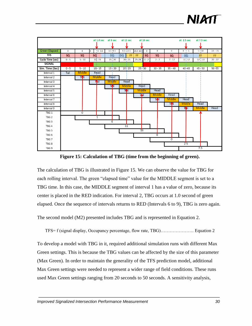
Figure 15: Calculation of TBG (time from the beginning of green).
The calculation of TBG is illustrated in Figure 15. We can observe the value for TBG for
each rolling interval. The green “elapsed time” value for the MIDDLE segment is set to a
TBG time. In this case, the MIDDLE segment of interval 1 has a value of zero, because its
center is placed in the RED indication. For interval 2, TBG occurs at 1.0 second of green
elapsed. Once the sequence of intervals returns to RED (Intervals 6 to 9), TBG is zero again.
The second model (M2) presented includes TBG and is represented in Equation 2.
TFS= f (signal display, Occupancy percentage, flow rate, TBG)…………………. Equation 2
To develop a model with TBG in it, required additional simulation runs with different Max
Green settings. This is because the TBG values can be affected by the size of this parameter
(Max Green). In order to maintain the generality of the TFS prediction model, additional
Max Green settings were needed to represent a wider range of field conditions. These runs
used Max Green settings ranging from 20 seconds to 50 seconds. A sensitivity analysis,

Improved Signalized Intersection Performance Measurement 31
investigating the effects of Max Green on the model accuracy, was developed and described
in the Analysis of Results chapter.
A second sensitivity test was run for the presence of premature gaps. As explained before, in
section 3.1.1.1, there are two classes of cycle failure; the first one when the maximum
discharge rate extends to the end of the max green and the phase terminates (max out), and
the second one due to a premature gap out. In the case of this research, the CRT identified the
first case as DQ-SQ easily, because the detectors recorded high occupancy and medium-high
flow rates when the phase terminated. Figure 16 shows the occupancy and volume
characteristics for PGO and the location of the DQ-SQ cases. In the lower graph, intervals in
the green region represent cycle failure due to a premature gap out event, while the intervals
in the red region belong to the ideal case in which the flow during the DQ state is not
interrupted. The figure clearly shows that DQ-SQ intervals that belong to the PGO case have
lower occupancy-flow rate values and are located in the medium-lower left side of the TFS
mix; this illustrates how the traffic characteristics change due to this PGO phenomenon.

Improved Signalized Intersection Performance Measurement 32
Figure 16: Data set with PGO and DQ-SQ location.
3.8 Calibration Data and Modeling in SPSS-Classification Regression Tree
The Classification and Regression Tree Model (CRT) is a binary decision tree algorithm that
splits data and produces accurate homogeneous subsets. This algorithm was popularized by
Brieman in 1984. This model can work for either categorical dependent variables
(Classification) or continuous dependent variables (Regression). In this research, the TFS are
the categorical dependent variables that are a function of dependent and continuous
predictors (signal indication, flow rate, occupancy percentage, and TBG).
No PGO
data points
PGO data
points

Improved Signalized Intersection Performance Measurement 33
The main purpose of performing these analyses via tree-building algorithms is to determine a
set of if-then logical (split) conditions that permit accurate prediction or classification of
cases given the independent variable data.
For each split (node), each independent variable (predictor) is evaluated to find the best cut
point (for continuous predictors) or the best groupings of categories (nominal and ordinal
predictors) based on an improvement score or reduction in impurity. This score or impurity is
a measure of the dependent variable variability. For each predictor, the split that produces the
best results is determined. Then the results of each of the predictors are compared, and the
predictor with the best improvement is selected for the split. The process is repeated
continuously until one of the stopping rules is triggered. These rules are:
A node reaches the maximum tree depth (CRT has 5 levels).
A node reaches the minimum impurity threshold set by the user, where a node is
“pure” if only one class is present (only one TFS in our case).
The number of cases in the terminal node is less than the minimum cases
specified for a parent or child node.
The impurity measure is given by a squared deviation (SD) for continuous variables. This
measure is defined as the within-node variance. For the nominal and ordinal variables, the
impurity measure is defined by the Gini measure. This value is based on squared
probabilities of membership for each class, where the various TFSs are the classes in this
research.
This procedure can be expressed in two steps:
- Segmentation: Identify data values for independent variables that belong to a specific
dependent variable value. For example, TFS tends to be SQ for the following
independent variable conditions:
Occupancy: 100%
Flow rate: 0 vph
Signal indication: Red

Improved Signalized Intersection Performance Measurement 34
TBG: 0
- Prediction: Create and formally establish the rules that create the tree based on the
split values found in the segmentation step for the predictors. The resulting tree would
be used to predict individual cases, given the predictor values.
As a conclusion, CRT splits the data into segments that are as homogeneous as possible with
respect to the dependent variable, in this case y=TFS. The classification tree will determine a
set of logical if-then conditions (instead of linear equations) for predicting or classifying
cases.
The advantages of using this model versus other statistical models were:
- Classification rules can be generated to test additional data sets.
- Other methods can test the accuracy of prediction but it is hard to define the cut
off values for future prediction.
- Misclassification cost can be defined to give more importance to more critical
classes, such as the DQ-SQ TFS.
- CRT can easily classify categorical and continuous variables combined.
- It is easy to visually explain categorical results. Highly visual trees enable you to
present results in an intuitive manner—so you can more clearly explain
categorical results to non-technical audiences.
For this research, the predictor variables that were researched were: Signal indication, Flow
rate, Occupancy, and TBG. A small sample of the input data is presented in Table 5.

Improved Signalized Intersection Performance Measurement 35
Table 5: Sample of the Data Set Input in SPSS
Figure 17 shows the first 2 parent nodes for the M2 model. The variable with less variability
and the one that provides the best improvement (30.5%) is TBG. This was selected among
the four available predictors. A cut off value of 0.4 seconds was estimated to split the data in
a binary form, and it is the value that provides the highest improvement or reduction in
impurity. Values below 0.4 seconds belong to the SQ TFS, with a classification accuracy of
98.9% (Node 1); values greater than 0.4 seconds belong to Node 2 where the rest of the TFS
are contained, since none of the stopping rules are triggered, the cases included in Node 2
will be split; and the process will continue until the 5th
level is reached.
TFS Occupancy Flow rate Signal TBG
SQ 100 0 R 0
SQ 100 0 R 0
SQ 100 0 R 0
SQ 100 0 R 0
SQ 100 240 R 0
SQ-DQ 92 720 G 1.1
DQ 85 1440 G 6.1
DQ 76 1920 G 11.1
DQ 75 2160 G 16.1
DQ-FF 49 1440 G 22.1
FF-SQ 47 960 Y 27.9

Improved Signalized Intersection Performance Measurement 36
Figure 17: CRT model nodes for TFS.
3.9 Validation with VISSIM and NGSIM Data
There are two validation date sets. The first one is based on VISSIM micro-simulation output
and the second one is field data obtained from processing the available NGSIM Atlanta raw
dataset. From these two sources, the same variables used in calibration were obtained to test
the validity and robustness of the model. To validate the model with field data, the NGSIM
Atlanta dataset was processed and aggregated to be tested with the rules generated by CRT
during calibration.
4. Analysis and Results
4.1 Model Calibration - Validation Results
Several models were tested in order to find the more reliable combination of variables to
predict TFS. The first section of this chapter is dedicated to the analysis of different models
considering additional variables. The second part tests the sensitivity of the most promising
model to max green values. It was the intention to test the relationship between the length of

Improved Signalized Intersection Performance Measurement 37
the max green parameter and the accuracy of the model. Since different max green values
vary in practice, significant sensitivity to max green settings may limit a method‟s
applicability to other scenarios with longer or shorter max green settings. The third section
presents the analysis of premature gap out events and the interpretation of the results in order
to better classify DQ-SQ TFSs (cycle failures).
4.1.1 Model Selection
It was found that the traffic information provided in terms of flow rate and occupancy
percentage can help to identify different TFS. The location of each TFS is presented in
Figure 18. It is possible to observe that the overlapping regions between the main TFSs are
the transitions between them. To help with the prediction of these states, additional variables
were required in the model. The next table presents the accuracy of the model considering 2
additional variables:
a) Signal indication: current indication displayed
b) TBG: time from the beginning of green indication
Figure 18: Main TFS location.
DQ
S
Q
FF
DQ-
FF SQ-
DQ
FF-
SQ
ALL
TFS

Improved Signalized Intersection Performance Measurement 38
Table 6: TFS Models
Model
TFS MODELS
M1 M2 Sample
size Flow, Occ, Sig Flow, Occ, Sig, TBG
CALIBRATION
DQ 91.1 92.3 784
DQ-FF 24.5 31.4 182
DQ-SQ 35.2 90.4 92
FF 78.9 77.1 266
FF-SQ 42.6 82.9 166
SQ 100.0 100.0 2372
SQ-DQ 65.2 99.4 304
Overall
Percentage 85.8 91.7 4166
VALIDATION
DQ 89.7 94.8 789
DQ-FF 29.7 35.2 175
DQ-SQ 38.1 77.8 90
FF 85.8 80.6 260
FF-SQ 41.8 79.2 182
SQ 100.0 100.0 2386
SQ-DQ 63.5 100.0 274
Overall
Percentage 85.6 92.3 4156
Out of the 3 proposed models, M2 shows an improvement of about 6.5% in accuracy, relative
to M1. Model 1 cannot identify the existence of the DQ-SQ state; therefore it was discarded
as a candidate for this selection.

Improved Signalized Intersection Performance Measurement 39
Table 7: Variable Importance for M2
Independe
nt
Variable
Importanc
e
Normalized
Importance
TBG .452 100.0%
Signal .315 69.7%
Occupancy .307 68.0%
Volume .281 62.1%
The correlation between the dependent variable and the predictors is shown in Table 7. As
expected, TBG has the highest significance when building the model. The model included
different cases where a phase terminates:
- Phase terminates after the queue is served (FF-SQ): The TBG value is greater than the
minimum green a smaller than the max green.
- Phase terminates long after the queue was served (FF-SQ): The TBG is equal or close
to the max green. Vehicle demand is sufficiently high to extend the phase until it
approaches or reaches the maximum green value.
- Phase terminates while serving the queue (DQ-SQ): The TBG value is equal to max
green. This is the case of a cycle failure due to a max out phase termination during
queue discharge.
These different tests calibrate the model more realistic, thus, comparable with existing
configuration in the field, especially for high speed approach with up-stream detectors.
4.2 Proposed Improvements
In order to improve the accuracy of the model, reduce false calls, and give a fair warning that
conditions are approaching critical, a new TFS named IMPENDING congestion was
introduced and was defined as the traffic state between a semi-congested condition (FF-SQ
with high occupancy and high flow rates) and severe congestion where the queue does not

Improved Signalized Intersection Performance Measurement 40
clear during green (DQ-SQ). It is important to note that the IMPENDING congestion state is
not a transition, because the state of the next interval is not known. Furthermore, it is
important to clarify that the FF-SQ state can vary from no-congestion to medium-high
congestion, presented in Figure 20. Free flow conditions vary in such a way because of
variations in the magnitude of the arrival flow rate. Data points within the blue diagonal lines
represent impending congestion, where both the FF-SQ and DQ-SQ regions largely overlap
each other. The definition of the boundaries for this new TFS is based on an observation of
the calibration dataset (no PGO data present) in Figure 19, where there is a region with
overlapping DQ-SQ and FF-SQ points. This overlap between states defines the boundaries
for the new IMPENDING state.
Figure 19: Defining the boundaries of the Impending Region - Calibration data.
In Figure 19, dots in green represent the FF-SQ intervals that were classified as FF-SQ
(correctly classified), dots in red are the ones that are FF-SQ intervals that were classified as

Improved Signalized Intersection Performance Measurement 41
DQ-SQ (Incorrectly classified). Diamonds in orange are DQ-SQ intervals that were classified
as DQ-SQ (correctly classified). Blue diamonds are DQ-SQ intervals that were classified as
FF-SQ state (incorrectly classified). There are two issues relevant to the definition of the
impending TFS:
- There is a substantial overlap of the DQ-SQ and FF-SQ TFSs.
- Many FF-SQ TFS intervals were misclassified and of these, all of them were
misclassified as DQ-SQ.
This suggests that the overlap in the conditions for the FF-SQ and DQ-SQ TFSs makes it
difficult for the CRT to distinguish between the two. The traffic operation conditions in
which it is difficult to differentiate between the two TFSs are when there is very little time in
which the FF-SQ TFS exists or when the flow rates during the FF TFS are so high that they
resemble conditions during the DQ TFS.
Once the region was defined Model 2 was recalibrated with the new TFS and the
classification results for the same data points shown in Figure 20 below.

Improved Signalized Intersection Performance Measurement 42
Figure 20: Defining impending region boundaries - calibration dataset.
The intervals between the two lines were reclassified as belonging to the IMPENDING TFS
and the equations for the two lines are as follows:
Upper limit: Occupancy % = -44.4 Flow-rate + 4200 ……………………… Equation 3
Lower limit: Occupancy % = -35.7 Flow-rate + 3500 ……………………… Equation 4
The results of the new model revealed that there is an improvement in distinguishing each
TFS. Defining a region between congested and semi-congested conditions gave the model
more flexibility, because the FF-SQ state can appear during a wide range of flow rates,
occupancy, and TBG values. There are two main reasons why the Impending TFS improved
the classification of TFS:

Improved Signalized Intersection Performance Measurement 43
- There are no longer overlapping regions between FF-SQ and DQ-SQ.
- There is a volatile range of conditions encompassed by the IMPENDING state where
it is difficult to distinguish between the two FF-SQ and DQ-SQ states.
Table 8: TFS Improvements for Model 2 with Impending
TFS Models M2 (without
PGO)
M2 +
Impending
(without PGO)
Sample
size
Calibration
DQ 94.4 74.3 784
DQ-FF 32.1 65.8 182
DQ-SQ 82.7 90.4 92
FF 77.9 61.7 266
FF-SQ 90 95.0 166
IMPENDING - 85.3 68
SQ 100 100.0 2372
SQ-DQ 99.4 99.7 304
Overall
Percentage 92.5 90.1 4166
Validation
DQ 93.2 74.1 789
DQ-FF 31.5 64.3 175
DQ-SQ 81.2 91.7 90
FF 79.3 57.7 260
IMPENDING - 73.1 78
FF-SQ 91.4 94.2 182
SQ 100 100.0 2386
SQ-DQ 100 99.7 274
Overall
Percentage 91.8 90.1 4156
The results in Table 8 show a similar overall performance for Model 2 relative to its
performance without the IMPENDING TFS. However, there are some marked

Improved Signalized Intersection Performance Measurement 44
improvements, primarily for the DQ-FF, DQ-SQ and FF-SQ TFSs. On the other hand, the FF
and DQ TFSs saw a reduction in accuracy.
Table 9 shows some promising trends and helps explain the implications for the TFSs
experiencing reduced accuracy. For example, when a wrong DQ-SQ prediction is present, it
is classified as IMPENDING which is more accurate than the previous incorrect
classification of FF-SQ. Similarly, when FF-SQ is misclassified, it is classified as
IMPENDING instead of DQ-SQ. A considerable improvement for the DQ-FF is observed in
Table 8. This occurred because in some cases DQ-FF occurs in the last 5 seconds, before
terminating the phase. The same is true of the DQ-SQ and FF-SQ TFSs. When traffic
conditions are heavy, but not yet congested, the flow rate and occupancy trends look similar
for these three TFSs. As a result, they were frequently misclassified. Including the
IMPENDING TFS, provided a classification to which cases representing the heavy-but-not-
yet-congested condition could be assigned with greater accuracy. This made the DQ-FF
classification more accurate, because the corresponding CRT criteria did not have to be so
broad as to include the borderline cases resulting from heavier traffic conditions. The same
reasoning applies for the corresponding DQ-SQ and FF-SQ improvements.
Results in Table 9 can also help describe the implications of the reduced FF and DQ
classification accuracy. For the DQ state, the misclassification error is not a significant issue
because the 200 out of the 224 misclassified cases were classified as DQ-FF. This is not a
serious departure from the true TFS and would not result in a decision to change traffic
control strategies. Implications for the FF classification error increase are similar, where the
large majority of the misclassified cases are classified as DQ-FF, as well. Again, this
misclassification error is still close to the true classification and is unlikely to result in an
inappropriate change in traffic control strategy, because there it does not represent a false
alarm that the system is failing.

Improved Signalized Intersection Performance Measurement 45
Table 9: Calibration and Validation Results for Model 2 with IMPENDING Region
Classification TFS with IMPENDING region
Sample Observed Predicted
DQ DQ-FF DQ-SQ FF FF-SQ IMPENDING SQ SQ-DQ
Percent
Correct
%
Calibration
(training)
DQ 649 200 5 7 2 2 8 0 74.3
DQ-FF 46 127 0 18 0 2 0 0 65.8
DQ-SQ 0 0 75 0 0 8 0 0 90.4
FF 13 104 0 219 10 2 7 0 61.7
FF-SQ 0 0 0 0 132 7 0 0 95.0
IMPENDING 0 0 6 0 4 58 0 0 85.3
SQ 0 0 0 0 0 0 2593 0 100.0
SQ-DQ 1 0 0 0 0 0 0 312 99.7
Overall
Percentage 15.4 9.3 1.9 5.3 3.3 1.6 56.5 6.8 90.1
Validation
(test)
DQ 648 190 6 22 1 1 6 1 74.1
DQ-FF 50 135 2 21 0 1 0 1 64.3
DQ-SQ 0 0 77 0 0 7 0 0 91.7
FF 15 90 2 172 6 4 9 0 57.7
FF-SQ 0 0 0 0 129 8 0 0 94.2
IMPENDING 0 0 9 0 12 57 0 0 73.1
SQ 0 0 0 0 0 0 2671 0 100.0
SQ-DQ 1 0 0 0 0 0 0 324 99.7
Overall
Percentage 15.3 8.9 2.1 4.6 3.2 1.7 57.4 7.0 90.1
Growing Method: CRT
Dependent Variable: TFS
4.3 Max Green Sensitivity Analysis
Table 10 shows the overall model accuracy for M2 model and the number of cases for each
treatment. For one test only one Max green setting was set for the simulation runs in VISSIM
(25 seconds). For the other test, five Max Green values were tested. Comparing the two test
results shows the sensitivity of the M2 model to variations in the Max Green setting.

Improved Signalized Intersection Performance Measurement 46
Table 10: Overall Model 2 Accuracy for Different Max Green Values
TFS MODELS
M2
Number of
Cases
M2
Number of
Cases
(only MaxG: 25sec) (MaxG: not 25
sec)
Flow, Occ, Sig,
TBG
Flow, Occ, Sig,
TBG
VALIDATION
DQ 93.7 789 85 175
DQ-FF 33.3 175 36.7 46
DQ-SQ 77.6 90 58.9 12
FF 80.6 260 74.5 127
FF-SQ 79.2 182 71.5 46
SQ 100 2386 98.6 506
SQ-DQ 100 274 96.7 64
Overall
Percentage 93.3 4156 88.4% 976
The results in Table 10 indicate that the M2 overall accuracy was reduced by 4.9%, meaning
that the model is sensitive to the different max green values which reduce its accuracy. The
prediction of DQ-SQ is quite sensitive to variation; on the other hand there is a small
variation for the estimation of other TFS such us DQ, DQ-FF, FF, and FF-SQ.
A Pooled t-statistic test was run to determine the significance of the accuracy differences for
each TFS (for the non-25 second set). Equations 5 and 6 were used to conduct the test.
Confidence interval:
21
21
11
nnstxx pc
………………………………………… Equation 5
Where: , : mean values
n1, n2: number of observations
tc: critical value for n1+n2-2 degrees of freedom

Improved Signalized Intersection Performance Measurement 47
Pooled standard deviation:
2
11
21
2
22
2
11
nn
snsns p
…………………………………………….. Equation 6
According to Table 11, only the DQ-FF and SQ TFS predictions are not significantly
different from those using the max green: 25 sec dataset. These results suggest that the
accuracy deteriorates significantly. This is especially problematic for the DQ-SQ, because it
makes it more difficult to identify cycle failure conditions for different max green settings.
Table 11: Pooled T-Test Results for Max Green Sensitivity for M2
Max Green:
25 sec
Max Green:
not 25 sec
TFS %
(x1)
Sample
Size
%
(x2)
Sample
Size Sp
x1-x2 TEST RESULTS
DQ 93.7 789 85 175 34.4 8.7 Significant
DQ-FF 33.3 175 36.7 46 16.3 3.4 NOT significant
DQ-SQ 77.6 90 58.9 12 9.3 18.7 Significant
FF 80.6 260 74.5 127 12.8 6.1 Significant
FF-SQ 79.2 182 71.5 46 16.5 7.7 Significant
SQ 100 2386 98.6 506 58.3 1.4 NOT significant
SQ-DQ 100 274 96.7 64 8.6 3.3 Significant
Ho: x1-x1 at 0.05 confidence level
The same analysis was performed for the M2 that includes the Impending TFS
(M2+Impending). Results in Table 11 show evidence that there is an impact in the accuracy
of predicting DQ-SQ state (-6%), and small increase in FF-SQ accuracy (+3.2%). The
statistical significance of these variations are shown in the polled t-test analysis in Table 13.

Improved Signalized Intersection Performance Measurement 48
Table 12: Max Green Sensitivity Analysis for M2+Impending Model
TFS Models
M2+Impending Number
of
Cases
M2+Impending Number
of
Cases
(only MaxG:
25sec)
(MaxG: not 25
sec)
Flow, Occ, Sig,
TBG
Flow, Occ, Sig,
TBG
Validation
DQ 74.1 789 83.4 175
DQ-FF 64.3 175 54.3 46
DQ-SQ 91.7 90 85.7 28
FF 57.7 260 55.9 127
FF-SQ 94.2 78 97.4 38
Impending 73.1 182 75.0 68
SQ 100.0 2386 100.0 2417
SQ-DQ 99.7 274 99.3 298
Overall
Percentage 90.1 4156 95.9 3197
Table 13: Pooled T-Test Results for MAX Green Sensitivity for M2+Impending
Max Green: Max Green:
25 sec not 25 sec
TFS
%
Sample Size
%
Sample Size Spa x1-x2 TEST RESULTS (x1) (x2)
DQ 74.1 789 83.4 175 13.5 9.3 Significant
DQ-FF 64.3 175 54.3 46 9.2 10 Significant
DQ-SQ 91.7 90 85.7 28 12.2 5.99 NOT significant
FF 57.7 260 55.9 127 12.0 1.8 NOT significant
FF-SQ 94.2 78 97.4 38 14.3 3.2 NOT significant
Impending 73.1 182 75.0 68 10.4 1.9 NOT significant
SQ 100 2386 100.0 2417 49.2 0 NOT significant
SQ-DQ 99.7 274 99.7 298 19.3 0 NOT significant
Ho: x1-x1 at 0.05 confidence level

Improved Signalized Intersection Performance Measurement 49
Only the DQ and DQ-FF states are statistically significant to the model M2+Impending. As a
conclusion we can state that there is a reduction in accuracy when predicting DQ-FF, on the
other hand there is an improvement in the DQ prediction. The DQ-SQ and FF-SQ states have
no significant impact when using the M2 + Impending model, meaning that the model can be
applied reliably for the tested range of Max green settings.
4.4 Premature Gap Out (PGO) Sensitivity Analysis
The inclusion of premature gap outs (PGO) in the model was previously mentioned in section
3.16. While comparing the validation results for Model 2 versus the ones for PGO-Only data,
a large change was observed. Table 14 shows the validation results from applying the CRT
rules generated to both validation data sets. Validation shows that there is 7.6% less accuracy
predicting FF-SQ and a decrease of 34.1% for DQ-SQ. Validating PGO data means testing
the model with data points that are not as easily identified as DQ-SQ. This is because, the
new PGO data points are instances where the DQ and DQ-SQ states are erroneously seen as
FF-SQ. They are categorized as FF-SQ, because during a premature gap out event, detectors
sense low flow rates and low occupancy, even though the traffic state is still DQ or DQ-SQ.
As a result, the CRT model tends to place the PGO data points in the FF and FF-SQ region as
shown in Table 14.
Table 14: Validation for M2 with and without the PGO Data
TFS Models
M2 (No PGO) Sample PGO Only Sample
Flow, Occ, Sig,
TBG size
Flow, Occ,
Sig, TBG size
Validation
DQ 93.2 789 72.2 194
DQ-FF 31.5 175 28.9 45
DQ-SQ 81.2 90 47.1 34
FF 79.3 260 84.9 73
FF-SQ 91.4 182 83.8 31
SQ 100 2386 99.1 428
SQ-DQ 100 274 96 50
Overall
Percentage 91.8 4156 85.3 855

Improved Signalized Intersection Performance Measurement 50
As for the Max green sensitivity analysis, an additional Pooled t-test was performed to see
whether the difference in accuracy for PGO data is statistically significant from cases without
PGOs present.
Table 15: Pooled T-Test Results for PGO Sensitivity M2
M2 model PGO only
(no PGO)
TFS
%
Sample Size
%
Sample Size Spa x1-x2 Test Results (x1) (x2)
DQ 93.7 789 72.2 194 14.4 21.5 Significant
DQ-FF 33.3 175 28.9 45 10.3 4.4 Significant
DQ-SQ 77.6 90 47.1 34 11.2 30.5 Significant
FF 80.6 260 84.9 73 10.2 4.3 Significant
FF-SQ 79.2 182 83.9 31 7.7 4.7 Significant
SQ 100 2386 99.1 428 21.6 0.9 NOT significant
SQ-DQ 100 274 96.0 50 7.3 4 Significant
Ho: x1-x1 at 0.05 confidence level
Table 15 shows that the reduction in the accuracy of prediction DQ-SQ is statistically
significant, also that the prediction of FF-SQ cases is positive for the model. This test proved
that the model is sensitive to the presence of premature gaps and tend to predict more FF-SQ
correctly.
The same analysis was performed for the M2+IMPENDING model. Table 15 shows the
accuracy of the tested model. There is a significant reduction of accuracy when predicting
DQ-SQ and FF-SQ states, the significance test for these results is presented in Table 16.
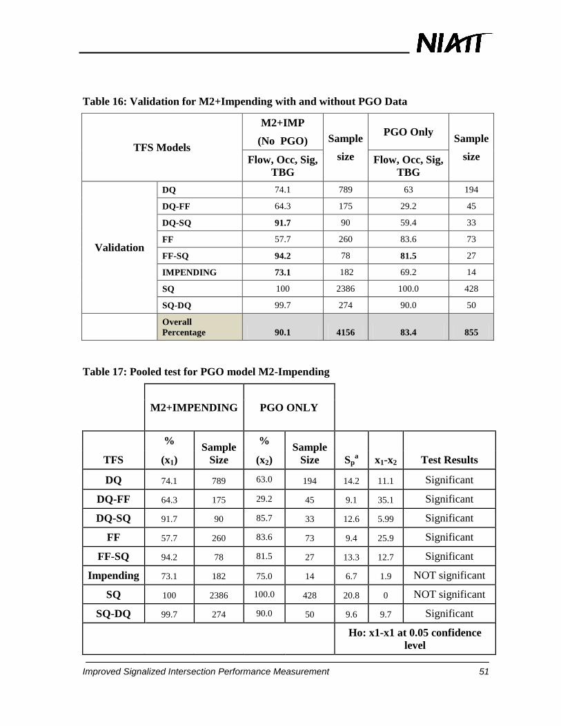
Improved Signalized Intersection Performance Measurement 51
Table 16: Validation for M2+Impending with and without PGO Data
TFS Models
M2+IMP
(No PGO) Sample
size
PGO Only Sample
size Flow, Occ, Sig,
TBG
Flow, Occ, Sig,
TBG
Validation
DQ 74.1 789 63 194
DQ-FF 64.3 175 29.2 45
DQ-SQ 91.7 90 59.4 33
FF 57.7 260 83.6 73
FF-SQ 94.2 78 81.5 27
IMPENDING 73.1 182 69.2 14
SQ 100 2386 100.0 428
SQ-DQ 99.7 274 90.0 50
Overall
Percentage 90.1 4156 83.4 855
Table 17: Pooled test for PGO model M2-Impending
M2+IMPENDING PGO ONLY
TFS
% Sample
Size
% Sample
Size Spa x1-x2 Test Results (x1) (x2)
DQ 74.1 789 63.0 194 14.2 11.1 Significant
DQ-FF 64.3 175 29.2 45 9.1 35.1 Significant
DQ-SQ 91.7 90 85.7 33 12.6 5.99 Significant
FF 57.7 260 83.6 73 9.4 25.9 Significant
FF-SQ 94.2 78 81.5 27 13.3 12.7 Significant
Impending 73.1 182 75.0 14 6.7 1.9 NOT significant
SQ 100 2386 100.0 428 20.8 0 NOT significant
SQ-DQ 99.7 274 90.0 50 9.6 9.7 Significant
Ho: x1-x1 at 0.05 confidence
level

Improved Signalized Intersection Performance Measurement 52
All TFS are significant, with exception of FF-SQ and Impending states. As a conclusion,
there is a limitation in the CRT procedure, for both models. When heavy vehicles and
inattentive drivers are prevalent at intersections, detector recordings do not accurately
represent field conditions. To address this weakness, advanced detector data are necessary.
Future analysis does not include PGO data, however the limitations of a stop bar based model
in the presence of premature gap out is a clear concern.
4.5 Field Implementation
There are previous steps that should be achieved and described in detail, for the model to be
implemented in the field:
The data logger should collect information from the controller and detector every tenth of a
second regarding:
- Signal information (from the controller); collect the present signal status and the
elapsed green time for the estimation of TBG.
- Detector actuations (from the loop detector); ON/OFF time stamps. Flag 1 if occupied
or 0 if not. Register the number of OFF times for estimation of volume counts for
short detectors.
Aggregate the above information in intervals of 15 seconds, according to the methodology
presented for the “15 second rolling interval.”
As the information is provided in terms of aggregated intervals run the classification rules
developed and produce output for each passing time interval. This logic could be
implemented in a feedback processor, which can process the output and determine the
necessary changes to implement in the real traffic controller.
4.6 Validation of the Model with NGSIM Field Data
Data available from the NGISM project were used to test Model 2 + Impending. Data
belonging to the through non-shared movements were considered. Data collected for this

Improved Signalized Intersection Performance Measurement 53
corridor of intersections does not include congested conditions for the recorded times. As a
result, there is no cycle failure (DQ-SQ) present in the results presented in Table 18.
Table 18: NGSIM Data Validation
Observed Validation NGSIM
DQ DQ-
FF
DQ-
SQ
FF IMP FF-
SQ
SQ SQ-
DQ
Total Correct Accuracy
DQ 42 16 58 42 72.4%
DQ-FF 12 22 34 68 22 32.4%
DQ-SQ 0 0 0 NA
FF 18 497 2 517 497 96.1%
IMPENDING 1 10 2 14 11 78
FF-SQ 6 62 68 62 91.2%
SQ 599 599 599 100.0%
SQ-DQ 5 60 65 60 92.3%
Dependent
Total
Intervals 1375 1282 93.2%
Variable: TFS
Overall
Accuracy 93.2%
The results above show a 93.2% accuracy of the overall model, showing that the model is
applicable to some field conditions. It is important to remark the accuracy for FF-SQ
prediction is 91.2%. This can be explained by the arrival of platoons from time frame 1600 to
1900 (end of yellow indication), as shown in Figure 21. This is not typical of the isolated
intersection operations simulated by VISSIM and used for calibration of Model 2. As seen in
the figure, the maximum flow rate is present during FF conditions, which can result in false
classification as DQ-SQ TFS. In the table above, six out of 68 FF-SQ cases where classified
as DQ-SQ, some of them belong to this platoon characteristic of flow.
The accuracy of DQ, DQ-FF, FF, SQ, and SQ-DQ is as expected from the previous
validation presented in Table 9. There is a considerable variation in terms of improvement
for the FF state, especially because the NGSIM flow rates have medium-low flow rates for

Improved Signalized Intersection Performance Measurement 54
most of the intervals belonging to this state. If we compare the field validation result with the
simulation data, the simulated contains more congested scenarios therefore there are more FF
intervals mixed with FF-SQ and DQ in the same region which makes it more difficult to
predict.
This suggests that even though the model accuracy for FF-SQ is good, situations like
coordination and platoon arrival should be studied in the future.
Figure 21: Presence of platoons in the field validation data.
5. Conclusions
5.1 Summary of Findings and Conclusions
Previous research tried to identify the different traffic conditions at actuated signalized
intersections. Most of this research focused on freeway operations. However, Hallenbeck
used detector information to obtain occupancy and volume counts to determine congestion
levels at signalized intersections. Hallenbeck‟s analysis is based in an hourly or daily
evaluation of performance, and so does not support a real time evaluation which can provide
feedback to the controller and/or operator to adjust timing settings for the current traffic
conditions.

Improved Signalized Intersection Performance Measurement 55
The primary purpose of this research was to present a real time method able to predict the
different TFS present during a cycle. This model was based on detector information and
improved with signal and timing characteristics. The summary of findings for this research is
as follows:
- Flow rate and occupancy information is not sufficient to define and predict the TFS.
DQ, DQ-FF, and FF can occur with the same traffic conditions. Therefore, there is a
need to include other variables in the model such us signal indication and TBG.
Model 2 was selected as preferred because it had the highest accuracy for predicting
DQ-SQ events.
- Two implementation of Model 2 were proposed that achieved over 90% accuracy in
validation tests. The Model 2 with no IMPENDING state does not perform as well,
but is less difficult to calibrate than Model 2 with the IMPENDING state.
- The model is sensitive to max green settings and should be further developed by
including different max green settings in simulation dataset.
- The method has a useful accuracy level for real-time traffic conditions. Therefore it
has potential to be implemented in the field to provide feedback to improve traffic
operations online.
- The model performance deteriorates when gaps inconsistent with that of a
discharging queue occur. As a result, the model will flag more false cycle failure
calls.
- The model is able to be recalibrated based on local conditions by using simulation of
the prevailing conditions.
- Including the IMPENDING state, improved the model performance for classifying
the most important states and provides a practical warning condition for traffic
operations that are approaching congested conditions.
5.2 Future Research
- Determine the accuracy of the model for intersections with different environments,
such as:

Improved Signalized Intersection Performance Measurement 56
o Detector placement and size; some intersections can provide upstream
information only or both stop bar and upstream
o Timing settings (max green and passage time)
o Presence of shared turning movements
o Intersection geometry, no presence of turning pockets (dedicated lanes)
- Effects of platoons from upstream intersections in the case of network based
intersections or corridors with intersections close to each other. An example of this is
the NGSIM validation data where it is possible to observe the arrival of platoon from
upstream intersections.
- Test the TFS logic using data collected from the field that includes congested
conditions.
- Test the proposed model‟s ability to provide feedback to operators and controller
algorithms.
- Address the presence of heavy vehicles and their impacts on the TFS model.
- Include data from advanced detectors to compliment the accuracy of the model, and
address the issue of PGOs.

Improved Signalized Intersection Performance Measurement 57
ESTABLISH SENSITIVITY OF METHOD FOR AUTOMATICALLY MEASURING DELAY
6. Introduction
The research in delay of this project was the continuation of the research started in the project
named “Development of New Actuated Signalized Intersection Performance Measurement
Methodologies Using Traffic Controller Input and Output Data.” In that project the delay was
measured by an automated method and the data were taken from both field and video
detection and those data were processed. In this project, from the collected data (the raw
data), erroneous data were filtered and then processed. In this report, all the procedures and
techniques that were used for the previous project (KLK120) are mentioned for the benefit of
the readers.
Delay is considered to be one of the important measures of effectiveness (MOE) to evaluate
the performance of signalized intersections. It is the sole basis that is used in the Highway
Capacity Manual (HCM) to determine the service quality (level of service) of different
movements at signalized intersections. Delay is difficult to directly measure from the field. In
many circumstances, the delay could be directly measured from the field, but it can be costly
due to the requirement of intensive data collection efforts and extensive human resources. It
is also most cost effective to employ an appropriate model and calibrate/validate the
performance of the model only relying on limited field data as input. However, field delay
measurements could prove valuable to traffic systems analysts, attempting to locate and
resolve problem areas in traffic systems. In addition, field delay measurements could help
inform travelers of more desirable routes. In this research, an automated delay measurement
procedure was accomplished based on the methodology presented by Kebab et.al. The
method is based on the point detection of vehicle events at different locations throughout the
intersection approach. The new vehicle data collection method and delay measurements were
expected to generate more convenient and detailed delay for different turning movements as
well as the through movement. However, when automating the procedure, it was found that
turning movement delays were not possible for shared lanes. So, the delay measures were
taken for exclusive turn lanes.

Improved Signalized Intersection Performance Measurement 58
This chapter discusses delay and it is organized into five sections including the introduction
section and they are as follows:
Problem statement,
Scope of research,
Description of automated delay methodology, and
Description of the data collection method.
7. Problem Statement
The problem addressed with this research is to increase the accuracy of the automated delay
measurement procedure and understand its sensitivity to detection error. Furthermore, the
automation should reduce the labor intensity typical to measuring delay.
8. Scope of the Research
The focus of this research was to measure approach delay (which includes stopped time
including the time lost when a vehicle decelerates from its original speed to a stop as well as
accelerating from the stop back to original speed) using an automated method that extracts
the delay from field recorded video data. This research describes an automated approach
delay measurement method with the intent to accomplish three major objectives:
1) Automated field data collection,
2) Increasing delay measurement resolution by measuring turning movement delays, and
3) Increasing the accuracy of field delay measurement.
To achieve these objectives, three delay measurement techniques were used for the research:
1) Automated delay measurement technique;
2) Vehicle tracking delay measurement technique (providing the benchmark approach
delay measurements and deceleration delay); and
3) HCM queue delay measurement technique, which were adjusted to approach delay by
adding deceleration delay.

Improved Signalized Intersection Performance Measurement 59
The automated delay measurement is based on point detection of vehicle events at different
locations on the intersection approach. The automated delay measurement results were
finally compared to vehicle tracking delay results, which represent the benchmark delay
values, and HCM delay measurement results. Then two statistical analyses Mean percent
error (MPE) and Mean absolute percent error (MAPE) were used to compare the correlation
between automated and benchmark delay measurements. Filtering techniques and sensitivity
analysis based on this automated delay measurement procedure are the primary focus for this
research. The development of the procedure was the focus of a previous research project, as
indicated earlier.
9. Methodology
9.1 Event Base Delay Measurement
To measure delay for this research, the automated delay measurement was applied by using a
video detection system to record the vehicle data and then followed the approach delay
measurement methodology that was proposed by Kebab [10]. The automated delay
measurement followed Kebab‟s methodology, which collected individual vehicle timestamps
at specific points for each approach. Three data collection points, Event X, Event 1, and
Event 3, were placed on each experiment approach to collect vehicle timestamps, from the
time vehicles entered the system until vehicles completely left the system (see Figure 22).
The locations and assumptions of the three proposed events are presented as follows.
Figure 22: Event locations for automated delay measurement.

Improved Signalized Intersection Performance Measurement 60
1) Event X is located at a point beyond the maximum queue length. The locations of
Event X remain the same for each approach regardless of the different time-of-day.
They can be varied by different approaches depending on the observed maximum
queue length at each approach.
2) Event 1 is located at a point where the turning movements have fully developed. It is
assumed that no lane change occurred after vehicles passed Event 1 until completely
through the intersection (Event 3). Assuming no lane change between these two
points allows the adoption of a first-in-first-out (FIFO) queue discipline for each
given lane. Because of the FIFO discipline, the nth vehicle to reach Event 1 will cross
Event 3 as the nth vehicle as well.
3) Event 3 is located at the stop line. The recorded timestamps for Event 3 are the times
that vehicles completely leave the stop line.
At the locations for the three events, the travel time for individual vehicles can be calculated
by comparing the timestamps of each event. The average travel time between Event X and
Event 1 was measured by using deterministic queuing principles. The average travel time
between Event 1 and Event 3 was measured by using FIFO queuing principles. Based on the
previous description, the travel time for turning movements also can be calculated by
comparing the timestamps at Event 1 and Event 3.
These travel time measurements were converted to delays by subtracting the corresponding
average free flow travel times, which were observed from the field (see Equation 7 from
Event X to Event 1 and Equation 8 from Event 1 to Event 3). The average approach delay
measurement can be determined by adding the average delay between Event X and Event 1
to the average delay between Event 1 and Event 3 (see Equation 9).
Delay calculation from Event X to 1
T
X
V
i
T
x
T
T
T
X FFTTititV
D
T
1
1
11
'
)'()'(1
'
Equation 7

Improved Signalized Intersection Performance Measurement 61
Where
T
XD 1' Average delay for automated delay measurement from Event X to Event 1
during time interval T
)'( 1 itT Video detection recorded time stamp of the thi vehicle for Event 1 during
time interval T
)'( itT
x Video detection recorded time stamp of the thi vehicle for Event X during
time interval T
'TV Video detection recorded total traffic volume in time interval T
T
XFFTT 1 Free flow travel time between Event X and Event 1 for time interval T
Delay calculation from Event 1 to 3
),,(,
31
1
13
,,
),,(,
31
,,
))'(())'((1
' RTTHLTT
V
i
TT
T
RTTHLT
RTTHLTT FFTTititV
D
TRTTHLT
Equation 8
Where
Average delay for automated delay measurement from Event 1 to Event 3
for different movements (LT, TH, and RT) (automated delay measurement)
Video detection recorded time stamp of the thi vehicle for Event 3 during
time interval T
Video detection recorded time stamp of the thi vehicle for Event 1 during
time interval T
Video detection recorded total traffic volume for different movements
during time interval T
Free flow travel time between Event 1 and Event 3 for different movement
time interval T
Average Approach Delay
3' X
approachD = T
XD 1' +
),,(,
31'RTTHLTTD Equation 9
))'(( 3 itT
))'(( 1 itT
),,(,
31
RTTHLTTFFTT
),,(,
31'RTTHLTTD
'
,,
T
RTTHLTV

Improved Signalized Intersection Performance Measurement 62
Where
3' X
approachD The average approach delay for automated delay measurement
T
XD 1' Average delay for automated delay measurement form Event X to Event 1
during time interval T
),,(,
31'RTTHLTTD
Average delay for automated delay measurement form Event 1 to Event 3 for
different movements (LT, TH, and RT)
9.2 Automated Delay Data Collection-Video Based Event Data Collection
The video detection device, AUTOSCOPE Rack Vision 8.3, produced by Econolite, Inc. was
used for applying the automated traffic data collection method. In the following sections, the
video detector placement guidelines and other related issues, which potentially influence the
accuracy of recorded data, are addressed.
Detector Placement Guidelines
Camera Height: According to the Intersection Video Detection Handbook, a minimum
height of 20ft is recommended in order to reduce adjacent lane occlusion and other factors
that could affect field-of-view. Hence, in order to record an appropriate field-of-view, taking
speed limit and the advance detector location into consideration, the camera height for this
research was 33ft; and it was placed on a stable telescoping mast to avoid above-average
errors that could be caused by unstable poles or masts.
Detector Zone Location: Detector zone locations followed the proposed event locations
except Event 3, which was located on the stop line. However, based on the field observation,
several drivers stopped on or beyond the stop line when they waited for the green signal
indication. This caused the video-detection device to record inaccurate timestamps. In order
to avoid such errors, two detector zones were placed at Event 3. One was on the stop bar and
the other was downstream of the stop bar and combined with a Boolean detector function to
control these two detector zones. The distance between two detector zones was chosen to be
equal to the average passenger vehicle length (15ft) in order to guarantee that time reported
by the detector is the time when the vehicle is completely leaving the stop bar.
Improved Signalized Intersection Performance Measurement 63
Detector Type: In any video data collection system, environmental factors and/or adjacent
lane occlusion easily affect the accuracy of collected data. Appropriate detector type
selection is important to mitigate the effect of these factors and increase the data collection
accuracy. Three types of detectors were used: speed detector, directional presence detector,
and cross lane presence detector. Different detector types were used at different event
locations to ensure the most accurate event timestamps.
For Event X and Event 1, the advance detector locations, a speed detector and a cross lane
presence detector combined with a Boolean detector function were used. After a series of
video detection exercises, the speed detector showed the best result for blocking the shadow
of adjacent lanes. The cross lane presence detector showed better performance and dealt with
different volume levels and generated more accurate results. Directional presence detectors
showed several detection errors, especially when the approach has successive slow moving
vehicles. Due to detector setting restrictions, the directional presence detector could not
detect every single vehicle and several miscounting errors occurred when two vehicles
occupied the same directional presence detector and were detected as a single vehicle with
one timestamp. Therefore, the directional presence detector seems not to be appropriate for
Event X and Event 1 detector placements.
For Event 3, stop bar detector location, a count detector and a directional presence detector
combined with a Boolean detector function were used. The detector function avoids
miscounted vehicles caused by shadows of opposite turning vehicles or calls that could be
caused by a tall vehicle. After adding the “AND” detector function for these two detectors, if
only one detector turns “ON” the vehicle is not detected for that lane of traffic. Hence, if the
count detector has been turned “ON” by a pedestrian and the directional presence detector
status is still “Off”, the call will not be recorded. Using a directional presence detector
instead of a cross lane presence detector avoids inaccurate detections such as pedestrians or
the shadows of other conflict approach‟s moving vehicles. On the other hand, when the green
period begins, the saturation headway and the vehicle move-up time between queued
vehicles could exceed two seconds which is greater than the detector detection time (from

Improved Signalized Intersection Performance Measurement 64
status turns “on” to “off”); therefore, the cross lane presence detector seems not to be
appropriate for Event 3 detector placement.
Another important detector placement issue for the Event 3 detector was the setting of the
left turn bay detector. This detector is easily affected by the shadows of opposite through lane
movement vehicles or conflict turning heavy vehicles. In order to improve the selectivity and
sensitivity of video detection, two parallel directional presence detectors combined with a
function “AND” were used. Figure 23 and Figure 24 show examples of the detection zone
layouts for two different intersection approaches.
Figure 23: Detector zone layout example (S.H 8 & Farm St).
Figure 24: Detector zone layout example (6th St. & Deakin St).

Improved Signalized Intersection Performance Measurement 65
Detector Mode In the AUTOSCOPE video detection device there is a useful function for
limitless large number of calls from different detection zones. These calls can be combined
and configured to control the intersection. Both pulse and presence mode detectors can be
used for user desired detector schemes. Different types of detectors which are in the same
detector channel can be combined by using different Boolean functions such as “OR” or
“AND”. This function benefits the video detection by allowing detection to occur only if
certain conditions are met, resulting in more accurate timestamps. For an example, refer to
the detector function “AND” in Figure 23. The Event 3 detection used a count detector
combined with a directional presence detector. After adding the “AND” detector function for
these two detectors, if only one detector turns “ON”, the vehicle is not detected for that lane
of traffic. For instance, if the count detector has been turned “ON” by a pedestrian, the call
will not be recorded. On the other hand, the detector function “OR” has a different
functionality. In this research, the “OR” detector function combined with the “AND”
function was placed in the two through lanes at the Event 1 location, as shown in Figure 24.
When the detectors of either lane were turned “ON” by way of the “AND” function, the
“OR” function will record one vehicle for the approach. This reduced the likelihood of an
approaching vehicle being counted multiple times because of triggering detection in both
lanes.
Figure 24 demonstrates the detection zone layouts. The setting and placement for each
detection zone or detector function are based on the video detection guidelines as described
before. All of the intersections for this research used a consistent detector zone placement
concept to record reliable traffic timestamps.
Sensitivity with Randomly Detection Error: Effect on Recorded Travel Time Estimation
Before applying the recorded vehicle data to calculate the travel time and approach delay, it
is essential to understand the relationship between detection errors and the final mean travel
time estimates. In this section, the investigation of the effect on recorded travel time when
detection errors are happening at random is presented. Throughout all detection error
sensitivity tests in this section, the recorded travel time represents the mean of the available
data. The percentages of detection errors were from 2% to 20% with a 2% increment. The

Improved Signalized Intersection Performance Measurement 66
recorded travel time results with different levels of detection errors were compared with the
recorded travel time with 0% detection error to test the sensitivity and accuracy of recorded
travel time. In addition, two different traffic volume levels, high and low, were used to
experiment the sensitivity of volume level and recorded mean travel time under different
detection error percentages. For both high and low volume conditions, the 15 minutes of
recorded data were used for sensitivity tests. An average of 120 vehicles was recorded in 15
minutes for high volume condition and an average of 20 vehicles for low volume condition.
The Figure 25 represents the results of sensitivity tests. From the trend of high volume
condition at the beginning, under different error percentages, the mean recorded travel time
points kept the close values to the travel time with 0% detection error. The range of
variations was between +3 to -1 seconds for mean recorded travel time comparisons under
high volume condition. When the percentage reached 18%, the mean recorded travel time
represented more variation in the results. As the detection error rate increases, the variation
significantly increases.
In comparison with high volume condition, the mean recorded travel times under low volume
condition experienced relatively high variations as compared with the recorded travel time
with 0% error rate. This phenomenon can be verified by comparing the trends of two linear
lines of low and high volume conditions. For each corresponding detection error percentage,
the low volume line kept a longer distance with X-axis than high volume line. It represents if
the low volume condition has the same detection error rate as high volume condition. The
low volume condition yielded a worse bias and an unreliable mean recorded travel time, and
influenced the final delay estimate. In the following section, a detection error filtering
method will be introduced. The error filtering method filters out these detection errors, and
adjusts the biases of recorded mean travel time and approach delay.

Improved Signalized Intersection Performance Measurement 67
Figure 25: The sensitivity with random detection error.
Automated Data Processing Principles
Raw data were collected, either through video detection or manual vehicle tracking. The raw
data were processed to obtain approach delay values by turning movements. Data processing
involved the following three steps:
1) Error checking and data filtering
2) Measuring delay from Event X to Event 1
3) Measuring delay from Event 1 to Event 3
4) Calculating individual vehicle approach delay
Step 1: Error Checking and Data Filtering
Error checking was accomplished by plotting the cumulative vehicles at upstream and
downstream detector locations (Event X to Event 3) versus time as shown in Figure 26. This
procedure identified vehicle event errors that may have occurred during data processing. In

Improved Signalized Intersection Performance Measurement 68
practice, errors were identified at one or more points where the two curves intersected. If data
from a certain time period showed errors, a data filtering process was applied to filter out
those erroneous detections. For data collected by video, each approach was analyzed an
average of 10 times.
0
5
10
15
20
25
30
35
40
45
50
55
60
65
0:00:00.00 0:02:52.80 0:05:45.60 0:08:38.40 0:11:31.20 0:14:24.00
Time
Cu
mu
lativ
e V
olu
me
Arrival_EventX
Event3
Figure 26: Cumulative vehicles versus time.
Erroneous Data Filtering Principles and Procedures
During the procedure of recording vehicle detection data, some environmental or
unpredictable factors affected the accuracy of the recorded data and erroneous data
potentially influenced the final delay results, so filtering of the data were required to
eliminate several detection errors. Three different types of errors were considered in the
analysis: 1) double detection, 2) unneeded detection, and 3) missed detection.
1. Double detection: With this error, the video detection equipment recorded two or more
detections when only one vehicle passed a detector. This type of error was the most
common detection error encountered in the analysis. Approximately 70% of detection
errors were related to double or multi-detection errors. Errors usually happened to long,
slow moving vehicles or vehicles that have vast differences in their light intensity.
Comparing the timestamps of both leading and following vehicles at each event, the
erroneous data were filtered out. The concept and procedures for filtering out these

Improved Signalized Intersection Performance Measurement 69
erroneous data are described in the following paragraphs.
From the microscopic car following perspective, the minimum safety headway of two
successive vehicles varies depending on the vehicles‟ speed. As the speed increases, the
minimum safe following distance increases. The speed limits for the intersections included
in this analysis are 25 mph for 6th
Street and Deakin Street and 35 mph for State Highway
8 and Farm Street. Several studies have examined minimum time headway based on field
data. For example, Louis (11) observed a minimum headway ranging from 1.5 to 2
seconds. For this analysis, the critical time headway between two consecutive vehicles
was assumed to be 1 second (5th
percentile). If the difference between two consecutive
timestamps was less than 1 second, one of the timestamps was treated as double detection
and, accordingly, deleted from the dataset. It can be seen from Table 19, the headway
between the first and the second vehicle in the unfiltered data is less than 1 second.
Therefore, one of the timestamps is identified as double detection and needs to be deleted.
After filtering out erroneous data, the actual headway between vehicle one and two is
32.91 seconds. The double detection filtering process is illustrated in Figure 27.
Table 19: Unfiltered and Filtered Data Comparison (Double Detection)

Improved Signalized Intersection Performance Measurement 70
Figure 27: Double detection filtering flow diagram.
2. Unneeded Detection: This error usually occurred when the detector was turned on (and
remained on) with no vehicle on the detector. A similar error occurred when the detector
recorded the adjacent lane‟s shadow as a vehicle causing an unneeded call.
The unneeded detection errors were hard to filter out as it was difficult to identify the source
of the error. The adjacent lane wrong detection was the only unneeded error that could be
filtered out by comparing the timestamps at the same event of different lanes. In this
research, based on the approach configuration presented in Figure 22, it is not possible for
the Event 1 detectors for the through right lane and the right turning pocket to be activated
simultaneously or with a time difference less than the minimum headway. Similarly, it was

Improved Signalized Intersection Performance Measurement 71
not possible for the Event 1 detectors for the through left lane and the left turning pocket to
be activated simultaneously. Depending on the sun‟s angle, one of these detections could be
identified as a detection error which can be eliminated from the recorded vehicle detection
data set.
In the example shown in Table 20, the 7th
timestamp of the TH movement is close to the
timestamp of the LT movement. Based on the previous first-in-first-out queuing discipline
and minimum time headway assumption, one of the timestamps is an unneeded detection and
checking with the sun‟s angle from the video, it could be eliminated. The unneeded detection
filtering process is illustrated in Figure 28.
The adjacent lane shadow unneeded detection error identification and filtering process
described here is limited to the lane channelization at the two intersections. If the approach
geometry is different from the one used in this analysis, the same data filtering method
cannot be applied.
Table 20: Unfiltered and Filtered Data Comparison (Unneeded Detection: Adjacent
Lane Shadow)
Movement Timestamp Movement Timestamp Movement Timestamp Movement Timestamp
TH 0:19:00.53 LT 0:20:01.17 TH 0:19:00.53 LT 0:20:01.17
TH 0:19:16.58 LT 0:20:36.44 TH 0:19:16.58 LT 0:20:36.44
TH 0:19:19.00 LT 0:20:41.65 TH 0:19:19.00 LT 0:20:41.65
TH 0:21:02.98 LT 0:21:02.23 TH 0:21:02.98 LT 0:21:02.23
TH 0:21:10.43 LT 0:22:38.57 TH 0:21:10.43 LT 0:22:38.57
Un-filtered Filtered

Improved Signalized Intersection Performance Measurement 72
Event 1(or 3) of RT (or LT) movement
vehicle timestamps
Event 1(or 3) of TH movement vehicle
timestamps
Comparing the timestamps
between RT&TH (or TH and LT) of diff.
Events
If have same timestamps
Check shadow
direction
Delete the detection caused by
adjacent lane‟s shadow No wrong detections occurred
No sa
me
Tim
esta
mps
Read event data of Event 1 RT movement & Event 1TH movement
(Or Read event data of Event 1 LT movement & Event 1TH movement)
(Or Read event data of Event 3 RT movement & Event 3 TH movement)
(Or Read event data of Event 3 LT movement & Event 3 TH movement)
Wrong detections
occurred
Figure 28: Unneeded detection flow diagram.
Missed Detection: Missed detection occurred when a vehicle passed a detector and the
detector zone was not activated. This error occurred randomly and could be attributed to
detection malfunction and/or environmental factors such as light and weather conditions.
Good detector zone placement and configuration can significantly reduce this error. No
filtering mechanism was developed for this error. Table 21 summarizes different detection
errors, and their potential problems for travel time/delay estimates.

Improved Signalized Intersection Performance Measurement 73
Table 21: Potential Sources of Errors in the Automated Data Collection
No. Possible error Filtering
/Mechanical Impact on average estimations
1
Vehicles in
analysis system at
the beginning of
interval
Un-filterable
This error will bias the travel time and approach delay
estimates. Based on the purpose, if data collection begins with
the same vehicle for Event 1 through Event 3 locations, then
the nth
timestamp at Event 1 & Event 3 locations will be the
same vehicle. If the residual queue already exists in the
analysis system, it will potentially affect the delay/travel time
estimates. The estimated results will be higher than the actual
ones. However, in this paper, comparing the first recorded
timestamps between downstream and upstream events can
determine the residual queues.
2 Double detection at
Event X Filterable
The accuracy of travel time/delay estimates between Event X
and Event 1.
3 Double detection at
Event 1 Filterable
The accuracy of travel time/delay estimates between Event X
& Event 1 and Event 1& Event 3.
4 Double detection at
Event 3 Filterable
The accuracy of travel time/delay estimates between Event 1
and Event 3.
5
Unneeded
detection at Event
X (caused by
shadow)
Filterable The accuracy of travel time/delay estimates between Event X
and Event 1.
6
Unneeded
detection at Event
1(caused by
shadow)
Filterable The accuracy of travel time/delay estimates between Event X
& Event 1 and Event 1& Event 3.
7
Unneeded
detection at Event
3 (caused by
shadow)
Filterable The accuracy of travel time/delay estimates between Event 1
and Event 3.
8
Unneeded
detection (caused
by equipment
failures)
Mechanical
Problem
It could have happened as different events and influenced
different parts of delay/travel time calculations.
9 Missed detection Unavoidable
Problem
It could have happened as different events and influenced
different parts of delay/travel time calculations. Creating a
good detector algorithm to decrease the probability of it
occurring is one of the options to avoid this error.

Improved Signalized Intersection Performance Measurement 74
Step 2: Calculating Event X to Event 1 Delay
Delays between Event X and Event 1 were calculated by using Equation 7 which is presented
in section 9.1. The concept for the delay calculation from Event X to Event 1 is the time
difference between two events for individual vehicle, adjusting by FFTT.
Step 3: Calculating Event 1 to Event 3 Delay
This delay measurement varies from previous Event X to Event 1 delay measurements which
is associated with all vehicles regardless of the movements. The delay process for Event 1 to
Event 3 needs to be considered for each turning movement. The validity of this association is
dependent upon the validity of the lane change assumption mentioned earlier. Because of the
timestamps of turning movements are recorded, delay can be associated with turning
movements. The delay measurement for Event 1 to Event 3 is using the same concept as
delay estimate for Event X to Event 1. Both of them are using recorded travel time subtracted
the FFTT. The Equation 8 represents the delay measurement from Event 1 to Event 3.
Step 4: Calculating Approach Delay
The approach delay (see Equation 9), including the delays form Event X to Event 1 and from
Event 1 to Event 3, is calculated by summing up the results of Equation 7 and Equation 8.
Both benchmark and automated delay measurements can apply Equation 9 to calculate the
approach delay.
10. Data Collection
10.1 Field Data Collection
The field data were collected by using a video-based data collection system. Data were
collected at two actuated signalized intersections which are located within the city of
Moscow, ID: one is a four-leg intersection, S.H. 8 & Farm St. (see Figure 29 - left) and the
other one is a three-leg intersection, 6th
St. & Deakin St. (see Figure 29 - right). The speed
limit for the three-leg intersection is 25 MPH and 35 MPH for the four-leg intersection. The
four-leg intersection, S.H. 8 & Farm St., operates in an actuated-coordinated mode and the

Improved Signalized Intersection Performance Measurement 75
coordinated phase is S.H. 8. The field data were recorded simultaneously for each approach
at the same intersection during the same time-of-day. Volume data were aggregated into a
15-minute time interval including non-peak and peak hours. Due to the limitations of
recorded field-of-views, data from only five approaches‟ were selected for measuring delay.
Twenty 15-minute time intervals were used in this analysis, which covers peak and non-peak
hour time intervals.
Figure 29: Intersection geometry S.H. 8 & Farm St (left) and 6th
St & Deakin St (right).
10.2 Manual Vehicle Tracking Data-Benchmark/Ground Truth Delay Data
For this research, vehicle data that were tracked and recorded using the manual vehicle
tracking method were treated as a benchmark, “true delay” data because these vehicle data
represented more accurate results as real field data. The manual vehicle tracking method
involved manual tracking and recording of vehicles‟ timestamps at different points
throughout the approach to the intersection. Vehicles were tracked through the intersection
approach progressing from the point they enter the intersection (Event X), to Event 1, then to
Event 3, where they depart the approach stop bar. The time stamps of each vehicle at these
three data collection points were then used to determine the travel time. The delay of each
vehicle was calculated by subtracting the FFTT from the corresponding approach travel time.
The average approach delay for each movement was calculated as the sum of the combined
approach delays from Event X to Event 1 and from Event 1 to Event 3 using Equation 10.

Improved Signalized Intersection Performance Measurement 76
),,(,
311
3 RTTHLTTT
X
X
approach DDD
Equation 10
Where:
3' X
approachD : Average approach delay
T
XD 1 : Average delay for from Event X to Event 1 during time interval T,
and
),,(,
31
RTTHLTTD : Average delay for manual delay measurement from Event 1 to Event
3 for different movements (LT, TH, and RT)
10.3 HCM Field Delay Measurement Procedures
Average queue delay for each approach was determined according to the procedures
described in HCM 2000 [11]. This method was based on direct observation of vehicle-in-
queue counts in a pre-defined time interval. The delays were manually calculated by
following a series of procedures recommended in HCM [11]. In HCM, the recommended
procedures used to collect and calculate the field delay is described in the following
paragraph.
Two observers are needed for applying the HCM delay measurement unless the volume is
light. One observer keeps track of the number of vehicles in queue for each cycle in the
survey period as well as the last vehicle in each lane that stops because of the traffic signal.
The second observer records the counts of total vehicles arriving during the survey period
and total vehicles arriving during the survey period that stop one or more times. Then, the
second observer adjusts the error that may have occurred by applying the sampling technique
as well as acceleration-deceleration correction factor. The HCM delay is computed by adding
the delay for vehicle-in-queue and the acceleration/deceleration correction delay.
However, in order to compare the queue delay measured using HCM procedures, the
approach delay estimated using the proposed method and the benchmark true approach delay
values obtained through manual vehicle tracking, the queue delay was adjusted to approach
delay. Reilly (4) defined the approach delay as the delay upstream of the intersection. It

Improved Signalized Intersection Performance Measurement 77
consists of three delay components: 1) stopped (queue) delay, 2) acceleration delay, and 3)
deceleration delay. The acceleration delay has two components: before and after the
approach‟s stop bar. In comparison to the delay components of the approach delay, the queue
delay in the HCM only consists of stop delay and acceleration delay. The queue delay can be
adjusted to approach delay by adding the average deceleration delay to the corresponding
queue delay. The equation for adjusting the queue delay to approach delay can be found in
Equation 11.
k
mnd
k
mnq
k
mnap ddd ),(),(),(
Equation 11
Where:
k
mnapd ),( : Approach delay at time interval k, at intersection n and for m movement,
k
mnqd ),( : Queue delay at time interval k, obtained from the HCM method, at
intersection n and for m movement, and
k
mndd ),( : Deceleration delay at time interval k (obtained using the vehicle tracking
method) at intersection n and for m movement
10.4 Free Flow Travel Time Measurement
As mentioned before, the proposed (automated) delay and vehicle tracking delay
measurement are calculated by subtracting the free flow travel time (FFTT) from recorded
total travel time for each vehicle. Free flow vehicles were identified as vehicles that drive
through the approach under unimpeded traffic conditions. For each time interval, the FFTT
from Event X to Event 1 and from Event 1 to Event 3 were recorded. For free flow travel
time from Event 1 to Event 3, the measurements were categorized by turning movement.
Thirty vehicles, which drove through the approach under free flow condition, were sampled
for each time interval. However, in some particular movements, the total volume did not
reach the desired sample size. In these cases, all free flow vehicles were observed and
recorded. Table 22 lists the observed FFTT for each intersection and approach.

Improved Signalized Intersection Performance Measurement 78
Table 22: Observed Free Flow Travel Time
LT TH RT
EB -- 7.5 8.5
WB 9 8.8 --
NB 13.3 11.3 12.1
WB 6.8 6 8.1
EB 9.1 7.9 9.8
FFTT (sec)
Lane group FFTT
25
35
Posted
speed
(MPH)
Approach
(--) Movement does not exist
11. Analysis of Results
In this section, collected and calculated data for this research are analyzed. This section is
divided into two sub-sections. Section 11.1 presents the reliability of automated delay
measurement. In section 11.1, automated delay measurement is compared with vehicle
tracking delay by using an Analysis of variance (ANOV) test. In section 11.1, three delay
measurements are compared. The three delay measurements that were used for this research
(Vehicle Tracking delay, HCM delay and Automated delay) are compared using two
statistical error measurements - Mean Percent Error (MPE) and Mean Absolute Percent
Error (MAPE).
11.1 The Reliability of Automated Delay Measurement
Comparing the vehicle tracking and automated delay measurements, the automated delay
measurement is easily affected its accuracy by erroneous detections. This result can be
proved in pervious sensitivity test, which was as the detection error rate increased, the final
mean recorded travel time/delay results were experiencing large biases. These errors could
occur in different circumstances and runs. Hence, it is essential to observe whether these
errors produced an unsettled mean recorded travel time for each run, and then influenced the
final delay estimate. After comparing the variation of two mean delays, automated mean
delay and actual mean delay, if the variation of two mean delays represented significantly
high, the automated delay measurement could not be able to replace the existing intersection
delay measurements, which are manual or other non-automated delay measurements.
However, if the mean automated delays represented as similar results as actual ones and only
few runs have relatively high variations, then, these detection errors were treated as randomly

Improved Signalized Intersection Performance Measurement 79
influencing the delay estimates only on some specific runs, and were not causing negative
effect to the final mean delay estimates. After that, the automated delay measurement can be
used as a reliable and capable method for measuring the delay in a more efficient way.
These detection errors could occur in all of the runs. However, based on the research
purpose, which was automated delay measurement, the numbers of detection errors were not
manually counted to observe the relationship between the number of detection errors and the
final delay results. The method that implies here is to test the relationship between number of
detection errors and the final delay results by using the run-delay diagram. The run-delay
diagram can be used to determine whether the errors are randomly influencing on some runs,
but still can yield similar final mean delays with actual ones. The run-delay diagram can also
be used to determine whether the errors are regularly influencing most of the runs and cause
negative effects to the mean delay results. This method will apply to all of the assigned
approaches with different time periods.
The run-delay diagram for westbound S.H. 8 and Farm St., for example, is presented in
Figure 30 and Figure 31. These two figures include two different time periods, non-peak hour
and peak hour. In these two diagrams, from the variations between two delay results, can
determine whether the variations are varied by different time-of-day/movements, and caused
high variations between two delay measurements. In Figure 30 and Figure 31, the lines of
automated delay measurement represented inconstant value for each run and movement. In
some runs, the automated delays represented statistically significant difference with actual
delays. The delays for run 5 and run 8 of left turn during non-peak hour, for example, have
approximately 5 seconds higher than the actual values. However, from the operational point-
of-view, the 5 second variation is not significantly affecting the intersection operation, and
furthermore, the difference between two mean delays of this particular phase is small.
Therefore, it can be concluded that the detection errors only randomly influenced some runs
and did not significantly bias the final mean delays. On the other hand, in terms of service
quality for this specific approach during non-peak periods, the level of service for these two
delay measurements were located at the same level, LOS=D. The LOS for the other two
movements represents the automated delay results have as same level of service as actual

Improved Signalized Intersection Performance Measurement 80
delay results. Similarly, the LOSs of automated delay measurement for three movements
during peak hour period have as same LOSs as actual delays. The LOSs for LT, TH, and RT
movements are B, A, and A respectively.
Average Delay LT TH RT
Actual Delay 43 15 4
Automated Delay 45 18 6
Diff. 2 3 2
LOS D B A
Figure 30: The WB of S.H. 8 & Farm St afternoon peak hour (example).

Improved Signalized Intersection Performance Measurement 81
Average Delay LT TH RT
Actual Delay 13 3 1
Automated Delay 16 5 3
Diff. 3 2 2
LOS B A A
Figure 31: The WB of S.H. 8 & Farm St afternoon non-peak hour (example).
In comparison with the average automated delays and actual delays, the mean automated
delays were slightly higher than actual ones for all of movements. However, the maximum
difference between two mean delays was around 3 seconds, and the 3 second delay
difference did not affect the intersection operation from an operational perspective. On the
other hand, from the trend of automated delay lines, the automated delays kept close to and
consistently different for most runs. Only few runs have relatively high variations. Therefore,
the detector errors are randomly influencing the delay estimates on some specific runs, and
still yield similar delays with actual ones. The automated delay measurement can be used as a
reliable and capable method for measuring the delay in a more efficient way.

Improved Signalized Intersection Performance Measurement 82
DEVISE A MEASURE TO COMMUNICATE THE PLAUSIBILITY OF OPERATIONAL IMPROVEMENT
This chapter discusses the green time utilization measure for this research. This chapter is
categorized into six sections. The first section (section 12) introduces green time utilization.
Problems addressed by this research are addressed in section 13. Section 14 explains the
scope of the research. Section 15 describes five steps that were used for the research. In this
section, the following issues are also presented:
Green time utilization performance measures and calculation of simple green time
utilization, call-normalized green time utilization and queue-normalized green time
utilization;
Resource availability and uses VISSIM and EXCEL/VBA for experiment;
Field consideration such as traffic conditions, intersection geometry, detector settings,
and passage time setting for the testing condition;
Experiment design (relationship between green time utilization and degree of
saturation(v/c); relationship between green time utilization and delay; green time
utilization as an index of unused capacity) for model development; and
Experiment design for testing.
Section 16 discusses the test results of green time utilization and section 17 presents the
corresponding analysis of the test results.
12. Introduction
Green time utilization (GTU) is one of the most important measures of performance for
signalized intersections. By definition, the percentage of the phase green time that serves
traffic is the green time utilization. However, this definition is applicable only for simple
green time utilization and simple green time utilization was used to evaluate the performance
of signalized intersection for a previous project entitled “Development of New Actuated
Signalized Intersection Performance Measurement Methodologies Using Traffic Controller
Input and Output Data.” In this project, intersection performance was evaluated using call-
normalization green time (CNG) utilization and queue normalized green (QNG) utilization.

Improved Signalized Intersection Performance Measurement 83
But simple green time utilization is also described in this report for reference and comparison
with the other two green time utilization.
The reasoning behind introducing two additional ways to calculate green time utilization is to
determine if more statistically sound relationships between GTU and degree of saturation can
be found.
13. Problem Statement
Problems related to green time utilization are listed below:
1. *Very little guidance is given on how this performance measure should be calculated
in real-time. It appears that its current forms available in controllers are not very
informative.
2. Forms available in centralized control software rely on specialized detector
configurations that are not practical for local actuated intersection control.
3. A systematic means for relating this measure to controller settings has not been
established.
4. Relationship between green time utilization and degree of saturation (v/c) is assumed
in the SCATs methodology, but is not well documented. In addition, it has not been
verified that it can be used as a surrogate for delay or to estimate delay.
5. *Appropriate green time utilization target values have not yet been determined. As a
result it is difficult to say whether or not a specific value is too high or too low.
6. *Methods for using green time utilization as an index to ascertain the unused capacity
available for improving intersection operations have not been investigated or
developed.
Not all problems relating to green time utilization are addressed here. However, problems
that are addressed in this report are indicated by an asterisk.
14. Scope of Research
The purpose for employing green time utilization measures is to make better judgments
regarding green time that is effectively and ineffectively used at signalized intersections. The
scope of this research is to establish how this performance measure should be calculated
using standard detector configurations. Methods for using the green time utilization

Improved Signalized Intersection Performance Measurement 84
performance measure for evaluating intersection traffic operations were developed. The foci
of these methods are listed below:
1. Relationship with v/c, and
2. Relationship with delay.
Finally, these methods were tested by applying them in a simulation environment in an
attempt to replicate field circumstances that might exist when endeavoring to evaluate and
improve intersection traffic operations. The primary focus of this research addresses the
problems stated in section 13.
15. Methodology
The methodology for this research is organized into five sub sections as listed below and
each of them is explained in detail is the subsection:
1. Green time utilization measures: this is a definition of the measure that was
investigated, assuming standard detector configurations.
2. Experiment/testing resources: this describes the relevant aspects of equipment and
software used to test methods for calculating the measure and methods for using the
measure.
3. Field circumstances: this describes (see 15.3) the assumed characteristics of test bed
intersections, including traffic conditions, detector configuration, intersection
geometry, and controller settings.
4. Experiment design for development: this describes the approximate experiment
design details such as the variables considered, their associated ranges, and the
assumptions needed. In addition, initial models relating dependent variables with
independent variables are also discussed. Resources used for obtaining data for
developing the models are also described section 15.4.
5. Experiment design for testing: this describes the approximate experiment design
details such as the variables considered, their respective ranges, and the error
measurements used. A description of how resources were used to execute the testing
is also provided in section 15.5.
15.1 Green Time Utilization Measures and v/c ratio calculation
There are two green time utilization performance measures considered in this research: call-
normalized green time utilization and queue normalized green time utilization. The definition

Improved Signalized Intersection Performance Measurement 85
of simple GTU is included in this section and represents previous research in an earlier
project (KLK120). However, this research represents the continuation of the project
KLK120. All the green time utilization measures (including the simple green time) and their
respective mathematical formulations are given in the following sub-sections.
Simple green time utilization
This is the percentage of a phase green time that serves the traffic. Simple green time
utilization is the proportion of a phase‟s active time that it serves traffic for the corresponding
protected movement.
Equation 12 describes how this representation of green time utilization should be calculated
using detector data for . The numerator of this equation is the sum of times that the active
phase detector is occupied, which is assumed to be the time that the phase is serving vehicles.
The variable id is „1‟ if the active phase detector is occupied and zero otherwise. In this
way, only the occupied detector times are included in the summation. The denominator is the
sum of detector intervals, whether the detector is occupied (on) or unoccupied (off) and
should be equivalent to the phase green time.
Ti
i
Ti
ii
t
td
GTU
Equation 12
Where
Active phase,
GTU Green time utilization for ,
i interval of time during which the detector status does not change for .
T contiguous set of detector status time intervals for the G interval of ,
id Detector status for the during detector interval i ( id = 1 if detector is on, zero
otherwise), and
it Time length of detector interval i during (seconds).

Improved Signalized Intersection Performance Measurement 86
Call-normalized green time utilization measure
Another way to look at green time utilization is to only consider green time during which
there is a call for service. In this case, the green time during which the active phase has a call,
or there is a serviceable conflicting call should be considered for determining whether or not
the green time is used effectively. So, normalized green time utilization can be defined as the
phase green time used to serve traffic relative to the time during which there is a call on the
active phase or a serviceable conflicting phase call.
A mathematical representation of how this form of green time utilization would be calculated
using detector data is shown in Equation 13. Similar to Equation 12, the numerator can be
assumed to be the time that the active phase is serving vehicles. However, the denominator is
different in that the only it that contribute to the summation are those during which either
the active phase detectors are occupied or detectors for a serviceable conflicting phase are
occupied.
Intervals where there is active phase detection are included in the first summation of the
denominator. Those intervals where there is a serviceable conflicting call, but no active phase
detection, are included in the second summation, because the value ii dd
sc is one.
Ti
ii
Ti
ii
Ti
ii
tdtd
td
GTU
sc
Equation 13
Where
i
scd Detector status for serviceable conflicting phases of during interval i (
i
scd = 1 if a
serviceable conflicting phase detector is on and there is no active phase detection,
zero otherwise).

Improved Signalized Intersection Performance Measurement 87
Queue-normalized green time utilization measure
Queue normalized green time utilization is the phase green time used to serve a queue
relative to the time during which there is a queue or a serviceable conflicting phase call.
A more discerning method for calculating green time utilization is to differentiate between
portions of the green serving a queue and those that are not, in addition to the presence of
serviceable conflicting calls. In other words, the green time is only effectively „used‟ while
serving a queue. Queue departure is measured by individual lane. Therefore, the queue is
being served as long as at least one lane is still serving the queue.
Ti
ii
Ti
ii
Ti
ii
tQtQ
tQ
GTU
sc
Equation 14
Where
iQ Queue discharge status for the during detector interval i (iQ = 1 if a queue is being
served, zero otherwise) and
i
scQ Detector status for serviceable conflicting phases of during interval i (
i
scQ = 1 if a
serviceable conflicting phase detector is on and no queue is being served by the active
phase, zero otherwise).
15.2 Experiment/Testing Resources
Resources that were brought to bear on this research were VISSIM simulation software and
Excel/VBA. These resources and the way that they were used are described in this
subsection. In this section, the use of VISSIM software to generate the experiment has been
narrated, and the data processing application by COM is described.
VISSIM simulation software
VISSIM was used to generate experiment and test data based on data output from
microscopic simulation. VAP was used to create the basic actuated intersection control logic,
where the following standard controller features were included: passage timer, min green

Improved Signalized Intersection Performance Measurement 88
timer, max green timer, yellow and all-red timers, gap-out, max-out, rest in green, eight
phase operation, simultaneous gap-out, dual entry, max recall, memory lock, and delay.
Application of green time utilization calculation methods were enacted on-line using VAP.
This enabled these methods to generate feedback to the VAP controller for application
testing.
VAP was developed so that the variables it and id were determined and thus available to
calculate green time utilization on-line. In addition, the *.ldp file settings were configured to
output green time utilization (GTU) as well as the variables. The variables iQ and
i
scQ are
not directly observed by detectors. As a result, they are only available in an approximate
form in VAP, similar to field circumstances.
The approximation to iQ and
i
scQ was made by calibrating an occupancy time based
indicator to represent the occupancy time pattern that best indicates the end of a queue. When
the indicator was comparable to current occupancy time patterns, the variable iQ was set to
zero for the following intervals and the variable i
scQ was set to 1 when appropriate.
GTU is an on-line calculation of green time utilization, calculated by VAP. The
variablesit ,
id , i
scd ,
iQ and i
scQ were on hand to calculate the green time utilization
measures off-line for purposes of verification.
The variables iQ and
i
scQ were not able to be calculated directly in the VAP. Therefore it
was necessary to create a variable 0t that would be used to determine if the queue had
cleared. If the stop bar detector experienced a gap time equal to or greater than the value of
0t then the queue would be deemed to have cleared the approach. The value for the variable
0t varies by approach speed of the intersection and is determined by measuring the detector
gap times following the end of queue and before the subsequent vehicle arrival or end of

Improved Signalized Intersection Performance Measurement 89
green. A sample of values for 0t is to be collected for each intersection. The value of 0t is
equal to the 85th
percentile of the collected sample values for use in the simulation.
The queue-normalized measure calculated on-line used approximate values for iQ and
i
scQ .
Therefore, it needed to be verified by comparing it to an off-line calculation that has access
to the vehicle file, which includes a field stating whether or not a vehicle has joined a queue,
based on a speed threshold. Given the vehicle queuing field in the vehicle file, the vehicle
data was processed in such a way as to determine the last vehicle discharging in queue and
the variables iQ and
i
scQ were determined more accurately and used as benchmarks.
Excel/VBA/COM
The bulk of data processing was executed within the Excel/VBA environment. The activities
completed in this manner are listed as follows:
1. Off-line calculation of v/c, using a macro written by Uriah Jones.
2. Off-line calculation of green time utilization performance measures.
3. Completing datasets off-line by creatingiQ , and
i
scQ , using the *.ldp and vehicle
files.
4. Execute multiple runs by varying the random number seeds and volumes.
5. It may be possible to determine iQ and
i
scQ on-line using COM, depending on the
objects that are available. However, this was not done in this experiment.
15.3 Field Circumstances
Field circumstances that were used for this research are commonly encountered. These
circumstances can be discussed in categories of traffic conditions, detector configuration,
intersection geometry, and controller settings. The following discussion describes these
conditions, with the intention of putting forth the default conditions. Based on the experiment
designs, these conditions were changed.

Improved Signalized Intersection Performance Measurement 90
Traffic conditions
The range of through traffic volumes for the phase in question was determined based on a
desired range for degree of saturation. This range was such that traffic conditions varied from
nearing congestion (v/c = 0.80) to capacity (v/c = 1.0). The respective volumes for these
conditions were determined by assuming fixed time control with green times set to the max
green values. Only passenger cars were present. Left turn volumes were set to 100 vph and
right turn volumes were set to 0 vph. Approach speeds ranges were set to 25, 35, and 45 mph.
No pedestrians were included in the simulation.
Detector configuration
The ITD standard for detector configurations was adopted and the VISSIM detector
configuration was updated to satisfy these conditions for each of the speeds stated in the
description of traffic conditions. Each detector had a dedicated channel to the controller, with
the exception of the detectors used for zone detection at the stop bar. Detectors did not cover
more than one lane.
Intersection geometry
Each approach has a one lane left turn pocket, a one lane right turn pocket, and two through-
only lanes.
Controller settings
The controller was set for phasing which included eight phases. The remaining settings were
set as listed below:
Min greens: 5 seconds
Max recall: off
Simultaneous gap-out: on
Dual entry: on
Memory lock: off
Delay: off
Max green: 30 seconds (through phase); 20 second (left turn phase)

Improved Signalized Intersection Performance Measurement 91
Yellow: (25 mph), (35 mph), and (45 mph)
Red: (25 mph), (35 mph), and (45 mph)
Passage Time settings
Three separate passage time settings were employed. The determination of the passage time
settings was based upon data collected for the end of queue gap time. For each intersection,
simulations were run and the stop-bar detector gap experienced between departure of the
queue and subsequent vehicle arrival or end of green was measured. The end of queue gap
times was then arranged into a cumulative distribution. From the cumulative distribution, the
50%, 85%, and 95% values were selected as the passage times to be used in the intersection
from which the end of queue gap times were collected.
The purpose of selecting three separate passage times was to provide passage time settings
that would create scenarios ranging across different phase termination conditions.
1. Green terminated too quickly to fully service the queue,
2. Green terminated just in time to service the queue, and
3. Green extends past the end of the queue.
15.4 Experiment design for model development
In this research three items were developed. Two are relationships between green time
utilization and degree of saturation (v/c) and delay. The third is a method for using green
time utilization as an index of unused capacity. Experiment design for each of these is
discussed below.
GTU (Green Time Utilization) vs. v/c and delay
The volumes needed to change in order to vary the delays for the turning movements (5 sec
to >60 sec). In addition, the v/c ratio needed to range from 0.80 to 1.0. There was no need to
exceed v/c=1 because at that point and beyond GTU would essentially be 1.0.

Improved Signalized Intersection Performance Measurement 92
To create these conditions in a simulation environment, the volumes were varied from 775 to
1100 vph; and the output data were processed using an Excel/VBA macro to determine the
v/c ratio and verify that the desired v/c ranges were satisfied. The VISSIM node output file
was used to verify that the desired delay ranges were satisfied. The resulting v/c and delay
values were included in the dataset used for analysis.
Each of the measures needed to be compared on the same time scale, which was the end of
green for a given phase. Green time utilization, v/c, and delay were all calculated and/or
aggregated for these times and a database was created with the following fields:
Run ID (sequence number)
Phase number (1 through 8)
Phase ID (sequence number)
Green end time (simulation seconds)
Approach (NB, SB, EB, WB)
GTU1
GTU2
GTU3
v/c
delay
GTU as an Index of Unused Capacity
PHASE GTU: The phase GTU describes the level of GTU for each phase of a given
intersection. Phase GTU represents the proportion of used green time for the phase.
INTERSECTION GTU: The intersection GTU describes the level of GTU for an entire
intersection, and is the total used time/unused time for all of the phases within the
intersection.

Improved Signalized Intersection Performance Measurement 93
It is believed that GTU is closely related to v/c ratio, and it may be used as an index of the
unused capacity of the intersection. In order to determine if GTU may be used as an index of
the unused capacity in this research, the GTU and v/c ratio was collected for each of the
scenario‟s described in section 15.3. Using the collected data, a linear relationship was
created between GTU and v/c ratio. If the relationship between GTU and v/c ratio is
determined to be statistically significant, then it may be concluded that GTU may be used as
a measure of unused capacity.
The higher the measured value of GTU the less unused capacity exists. Therefore, a target
value range of GTU could be determined based on the desired range of v/c ratio for the
intersection. And the controller could be modified to allow input based on the value of GTU.
If the GTU is below the desired target range, the controller settings could be modified to
increase the GTU until it falls within the desired range. Conversely, if the measured GTU
was too high, then controller settings could again be modified to lower the GTU.
15.5 Experiment design for testing
A number of scenarios were created to conduct the experiment. This section outlines the
inputs for the scenarios and the method for determination of relationships from the
experiment data.
Simulation Input
For each scenario given in the section 15.3, five separate simulations were run. Each
simulation consisted of 5 minutes of run time before recording occurred, 15 minutes of
recorded simulation, and ended with 5 minutes of run time in which no data were collected.
Signal control data and values for Delay, Simple GTU, Call-Normalized GTU, and Queue-
Normalized GTU were recorded for each simulation in the *.ldp output files from VISSIM.
Following the simulations, data were collected out of the *.ldp files by Excel macros. Values
for GTU were calculated on-line for each cycle.
Values of GTU were recorded at the end of each cycle; a typical simulation would have
approximately 10 cycles for the 15 minutes of recorded simulation time. To determine the

Improved Signalized Intersection Performance Measurement 94
GTU value for a simulation run, all recorded GTU values for the simulation were averaged.
This was calculated separately for each measure of GTU.
Simple GTU
The values collected in the *.ldp files were used to establish a relationship between GTU, as
determined by the simple measure, and v/c ratio as well as delay. The collection and
evaluation of the data was accomplished as outlined above. Based on the collected data, a
linear relationship was established for each GTU measure against both v/c ratio and delay.
The quality of the relationships was assessed using the Data Analysis package in Excel to
determine the level of significance for each relationship.
GTU – Call-Normalized, Queue Normalized
The values collected in the *.ldp files was used to establish a relationship between GTU, as
determined by the simple measure, and v/c ratio as well as delay. The collection and
evaluation of data will take place for all three measures of GTU as outlined above. Based on
collected data, a linear relationship will be established for each GTU measure against both
v/c ratio and delay. The quality of the relationships will be assessed using the Data Analysis
package in Excel to determine the level of significance for each relationship.
GTU as surrogate for v/c ratio and/or delay
Based upon the quality of the relationship between GTU and v/c ratio and GTU and delay,
GTU was used as a surrogate for v/c ratio and/or delay. If the data collected shows that there
were a highly significant relationship between GTU and either v/c ratio or delay, then it may
be allowable to use GTU to determine an approximate measure of either v/c ratio or delay.
The GTU measure was evaluated in order to determine its appropriateness for use as a
surrogate of v/c ratio or delay.
16. Simulation Results
The resulting data from the simulations was analyzed with the Excel Data Analysis package,
and linear relationships between Delay and GTU, and v/c ratio and GTU were established.

Improved Signalized Intersection Performance Measurement 95
Table 23 and Table 24 show the results of the data analysis. Relationships follow the form of
the following equations;
GUcv 10/ Equation 15
GUDelay 10 Equation 16
Table 23 and Table 24 also include the adjusted R-square values, significance, and t-test for
both the intercept and independent variable (X variable); which are included to show the
quality of the relationship.
Table 23: Regression Analysis of GTU vs. Degree of Saturation
v/c ratio vs. GTU t-test
Performance Measure β0 β1 Adj. R2 Significance Intercept X Variable
Simple GTU 59.282 26.647 0.144 3.46*10-6
12.399 4.845
Call-Norm GTU 59.926 33.55 0.237 1.235*10-9
11.86 6.536
Queue-Norm GTU 29.196 43.252 0.1897 7.75*10-8
4.418 5.69
Table 24: Regression Analysis of GTU vs. Delay
Delay vs. GTU t-test
Performance Measure
β0 β1 Adj. R2 Significance Intercept X Variable
Simple GTU 73.289 0.403 0.0583 0.00278 24.37 3.048
Call-Norm GTU 72.303 0.43 0.0691 0.00121 24.45 3.308
Queue-Norm GTU 59.699 0.309 0.0117 0.110143 13.637 1.608
To be significant a model must have a significance value of <0.05. The relationship between
Queue-Normalized GTU and Delay was determined to be insignificant (see Table 24) due to
high significance value and low t-stat values.
17. Analysis of Data
Throughout this section, figures are used to represent the results of the simulation runs
comparing degree of saturation and delay to GTU. Each data point on the graphs represents

Improved Signalized Intersection Performance Measurement 96
the averaged GTU values for all cycles during a simulation, there were approximately 10
cycles per simulation run. Data from all scenarios were used in the creation of the plots and
the subsequent data analysis. Thus relationships were established independent of speed of
approach or passage time.
17.1 Simple GTU
The simple GTU is the basic measurement of green time utilization that was employed in the
experiment. A linear relationship between v/c ratio and GTU was found. Although a high
level of variablity was measured as the v/c ratio decrease below 0.8. All data points were
determined from one approach whose volume was varied to obtain a range of v/c ratios,
while the remaining approaches were subjected to a constant high volume. At a low volume,
the measured approach may have had the green extened due to the higher traffic flow on the
opposite approach. Thus creating artificially low values for GTU. Alternatively, if low
passage times were used then the green may be artificially shortened, thus yielding the high
GTU values seen in the low v/c ratio range.
It would appear that the simple GTU measure approaches a maximum value as it nears 95%.
Since GTU is measured over a period of approximately 10 cycles, and the more cycles that
are included increase the liklihood that a cycle will occur without fully utilizing the green
time, a max attainable value of less than 100% was expected.
Figure 32: Simple GTU vs. degree of saturation.

Improved Signalized Intersection Performance Measurement 97
The horizontal lines seen in Figure 32 represent the GTU range corresponding to a v/c ratio
of 0.9 to 0.95. A range of 83% to 85% GTU corresponds to a v/c ratio of 0.9 to 0.95. This
range is representative of traffic conditions nearing capacity.
Figure 33: Simple GTU vs. delay.
As seen in Figure 32 and Figure 33, GTU increases both with an increase in v/c ratio and also
an increase in Delay. An increase in GTU as v/c increases was expected, for with higher
demand volumes there tends to be longer queues, and resultantly higher number of vehicles
using the intersection. Similarly, an increase in Delay represents an increase in demand on
the intersection.
The variability of the GTU measurement was significantly higher in the Delay model.
Overall, the higher variability of the Delay model is attributed to the inherent variability in
delay calculations. Despite the increase in variability, the Delay model still proves to be
statistically significant. Unlike the v/c ratio model, the Delay model exhibits no increase in
variability as the Delay decreases.
17.2 Call-Normalized GTU
Although similar to the Simple GTU measure, the Call-Normalized GTU measure also takes
into account the demand on the other approaches. As can be seen by comparison with the
Simple GTU measure, in Table 23 and Table 24, the results are very similar. This is due to

Improved Signalized Intersection Performance Measurement 98
the similarity with which the GTU was measured. Call-Normalized GTU also includes
demand on the adjacent approaches, so that green time is defined as “not being used” only if
there is a call on a conflicting phase and no vehicle being served on the active phase. When
an intersection is operating under high demand, a call on a conflicting phase is almost
continuous. So, variations between the Simple GTU and Call-Normalized GTU are only
expected at low v/c ratios. Since all of the simulations were run at high v/c ratios, there was
not much difference measure between Simple GTU and Call-Normalized GTU, which was
expected.
Figure 34: Call normalized GTU vs. degree of saturation.

Improved Signalized Intersection Performance Measurement 99
Figure 35: Call normalized GTU vs. delay.
The Call-Normalized GTU range corresponding to a v/c ratio range of 0.9 to 0.95 is 82% to
85%. As the Call-Normalized GTU nears 85%, the intersection is nearing capacity with v/c
ratio approaching 0.95. This range of CNG (82% to 85%) could be used as an indicator of
when traffic conditions are approaching saturated conditions
Figure 34 and Figure 35 represent GTU vs. v/c ratio and GTU vs. Delay respectively. As is
consistent within the previous experiment, the delay model experiences a higher variability
than that of the v/c ratio model. Additionally, GTU increases with the increase of both v/c
and Delay.
The Call-Normalized GTU measure contains the least variability of the measures used in this
experiment. As a result of the elimination of the variability at lower v/c ratios the Call-
Normalized GTU provides a more accurate measurement of GTU than the Simple GTU
measure.
17.3 Queue-Normalized GTU
The Queue-Normalized GTU measure (QNG) results in the lowest calculated values for
GTU. Also, it has the largest variability of the GTU measures employed in the experiment.
Despite the higher level of variability, the Queue-Normalized measure provides a statistically

Improved Signalized Intersection Performance Measurement 100
significant measure of GTU based upon v/c ratio. The Delay model created using the Queue-
Normalized measure was found to not be statistically significant, and does not justify further
consideration.
Figure 36: Queue-Normalized GTU vs. degree of saturation.
Figure 37: Queue-Normalized GTU vs. delay.
The Queue-Normalized GTU range corresponding to the v/c ratio of 0.9 to 0.95 is much
lower than the Call-Normalized GTU measure. A GTU range of 68% to 71% corresponds to

Improved Signalized Intersection Performance Measurement 101
the v/c ratio range of 0.9 to 0.95. The lower range found here is expected due to the overall
lower values for GTU measured.
The results of the simulation runs can be seen in Figure 36 for the v/c ratio model with
respect to the Queue-Normalized GTU. The increase in variability of the QNG results from
the way in which it is measured. By using the variable 0t to define the end of queue, the
varying nature of queue departure will result in errors in GTU measurement. A queue which
is measured to have been serviced earlier, in reality will result in a biased low GTU value,
while a queue which was measured to have extended past the real queue departure time will
result in biased high GTU values that were measured.
The QNG GTU is significantly lower than either the Call-Normalized or Simple GTU
measures because once the queue is determined to have departed, all remaining green time is
classified as not-used. In contrast, the other two GTU measures continue to record green time
as used as long vehicles continue to cross the stop bar.

Improved Signalized Intersection Performance Measurement 102
DOCUMENTATION AND PUBLICATION
TRB PAPER (submitted): Automated delay measurement w/ study of error effects.
ASCE PAPER (in progress): Detecting traffic flow states using basic actuation
detection and signal status.
18. Conclusions and Future Research
This research has provided insight into the various characteristics associated with the Green
Time Utilization performance measure and its relationship to degree of saturation. It was
found that a simple regression model can be used to provide a statistically significant
relationship between GTU and v/c. In addition, it was found that for the call-normalized
GTU of between 82% and 85% corresponds to a v/c value in the range of 0.90 to 0.95.
The call-normalized and queue-normalized GTU measures do offer additional information
relative to the simple GTU measure. However, the simple GTU measure works similarly, or
better, as a surrogate for v/c or delay.
Future research should evaluate using the SCATS degree of saturation measurement method
to determine GTU in a fashion that is more consistent with the definition of v/c. The
continuously-updated saturation gap could be used to better inform when queues have been
served and for setting passage times. Finally, research should also define how GTU be used
as a feedback measure to inform off-line traffic control strategy modifications.

Improved Signalized Intersection Performance Measurement 103
BIBLIOGRAPHY
[1] Mark Hallenbeck, J. I. (2008). Arterial Performance monitoring using sensor data.
Washington DC: Transportation Research Board.
[2] Akcelik, R., & Besley, M. (2002). Queue discharge flow and speed models for signalized
intersections.
[3] Andrew Nichols, D. B. (2001). Design Guidelines for deploying Closed Loop Systems.
Purdue University, West Lafayette.
[4] Darcy M. Bullock, J. V. (2007). Performance of Modern Stop Bar Loop Count Detectors
over Various Traffic Regimes. TRB paper 07-1090.
[5] Department, I. T. (2008). Traffic Manual. ITD.
[6] Edward J. Smaglik, A. S. (2006). Event Based Data Collection for Generating Actuated
Controller Performance Measure . TRB paper 07-1094.
[7] Michael Kyte, H. W. (2008). Effect of Detector and Timming Parameters on Operation of
Cross Street of Isaolated Intersections, MOST Project. Moscow, ID: NIATT.
[8] Sharma, B. a. (2007). Input-Output and Hybrid Techniques for the Real Time Prediction
of Delay and Maximum Queue Lenght at a Signalized Intersection. TRB paper.
[9] SPSS. (2007). SPSS Classification Trees™ 13.0 Manual. . SPSS.
[10] Kebab, M, M.P. Dixon, A.Abdel-Rahim. Field Measurement of Approach Delay at
Signalized Intersections Using Point Data. Journal of the Transportation Research Board. No.
2027, Transportation Research Board of the National Academies.
[11] Highway Capacity Manual (200) Washington, D.C., Transportation Research Board.
[12] Kell, J., Fullerton, I., and Mills, M., Traffic Detector Handbook, Second Edition, Federal
Highway Administration, Washington, DC, 1990.
[13] Chen, L., and May, A., “Traffic Detector Errors and Diagnostics” Transportation
Research Record 1132, TRB, Washington, DC, 1987, pp 82-93.
[14] Coifman, B., “Using Dual Loop Speed Traps to Identify Detector Errors” 990550, TRB,
Washington, DC, 1999.
[15] Jacobson, L, Nihan, N., and Bender, J., "Detecting Erroneous Loop Detector Data in a
Freeway Traffic Management System," Transportation Research Record 1287, TRB,
Washington, DC, 1990, pp 151-166.

Improved Signalized Intersection Performance Measurement 104
[16] Prevedouros et al. , video incident detection tests in freeway tunnels, TRB, national
academics, Washington D.C, 2006.
[17] Hidalgo, Dario et al. Effect of traffic detection errors on the accuracy of volume reports,
National Traffic Data Acquisition Conference, Albuquerque, New Mexico 1996.
[18] US DOT-FHWA, “Traffic Monitoring Guide”, Publication No. FHWA-PL-92-0 17,
1992.
[19] Wright, T et al. Variability in continuous traffic monitoring data, National Traffic Data
Acquisition Conference, Albuquerque, New Mexico 1996.
[20] Bonneson, J and Abbas, M, Video Detection for Intersection and Interchange Control,
FHWA/TX-03/4285-1, 2002.
[21] Bonneson, J and Abbas, M, Video Detection Handbook, FHWA/TX-03/4285-3, 2003.

Improved Signalized Intersection Performance Measurement 105
APPENDIX
1.1 Algorithms
1.1.1 TFS macro
Extract data from Vehicle record file (*.fzp)
Filter vehicle information per lane
Identify vehicles joining the queue “in queue” Speed < 5mph
Import signal information from SIGNAL macro: # cycles, signal lengths
Track all vehicles cycle by cycle
Identify the HEAD and TAIL of queue
Track HEAD and TAIL along each cycle
over the entire simulation run
Verify that HEAD and TAIL cross the
stop bar
Compare HEAD/TAIL location versus stop bar location
Determine TFS for each simulation second
NO
YES

Improved Signalized Intersection Performance Measurement 106
1.1.2 SIGNAL macro
Extract data from signal control file
(*.ldp)
Collect number of cycles and cycle lengths
Determine the length of each signal
indication
Determine the elapsed time for each
signal indication
Collect the beginning and end time
stamps for each signal indication for
each cycle

Improved Signalized Intersection Performance Measurement 107
1.1.3 DETECTOR macro
Extract data from Data collection files (*.mer)
Read time step for each vehicle
along time
Filter vehicle information by lane
Filter vehicle information by data
collection point (detector)
Import signal information from macro
SIGNAL
Generate ON/OFF times for each tenth
of the second along simulation time.
Obtain vehicles #, ON/OFF time, vehicle
occupancy

Improved Signalized Intersection Performance Measurement 108
1.1.4 OCCUPANCY AND FLOW RATE macro
Import signal information and cycle #
from SIGNAL macro
Import ON/OFF times and occupancy
from Detector macro
Import TFS states from TFS macro
Generate TFS elapsed time
Generate Occupancy flag for each tenth of
the second
Determine Green Elapsed time
Plot simulation time for each tenth of
second
Aggregate data based on the 15 rolling
interval
Determine TBG, Signal and TFS for each
15 second
Generate Flow-Occupancy plots showing
the location of each TFS

Improved Signalized Intersection Performance Measurement 109
1.2 CRT trees for chosen models.
Classification Tree for Model 2

Improved Signalized Intersection Performance Measurement 110
Classification Regression Tree for Model 2 with IMPENDING region