open source natural language processing - worcester
TRANSCRIPT

0
PROJECT NUMER: CS-GXS-1001
Open Source Natural Language Processing
A Major Qualifying Project Report submitted to the Faculty of the
Worcester Polytechnic Institute
in partial fulfillment of the requirements for the Degree of Bachelor of Science by
Kara Greenfield
Sarah Judd
4/29/2010
Professor Gábor N. Sarkozy, Major Advisor
Professor Stanley M. Selkow, Co-Advisor

1
Abstract
Our MQP aimed to introduce finite state machine based techniques for natural language processing
into Hunspell, the world’s premiere Open Source spell checker used in several prominent projects
such as Firefox and Open Office. We created compact machine-readable finite state transducer
representations of 26 of the most commonly used languages on Wikipedia. We then created an
automata based spell checker. In addition, we implemented an transducer based stemmer, which
will be used in the future of transducer based morphological analysis.

2
Acknowledgements
We would like to thank the following people for helping us in varying ways throughout the project:
Professor Sárkózy Gábor - main Advisor
Professor Stanley Selkow - co-Advisor
Kornai András - SZTAKI liaison
Varga Dániel - MOKK liaison
Zsibrita János - original code developer
Richard Farkas - original code developer
Recski Gábor - SZTAKI Colleague
Zseder Attila - SZTAKI Colleague
Erdélyi Miklós – SZTAKI Colleague
Szabó Adrienne - SZTAKI Colleague
Daniel Bjorge - C debugging
Worcester Polytechnic Institute

3
Table of Contents
Abstract ................................................................................................................................................... 1
Acknowledgements ................................................................................................................................. 2
Introduction .......................................................................................................................................... 10
Chapter 1: Background ......................................................................................................................... 12
Affix and Dictionary Files .................................................................................................................. 12
Dictionary File ............................................................................................................................... 12
Affix File ......................................................................................................................................... 13
Finite State Automata ....................................................................................................................... 14
Deterministic Finite State Automata ............................................................................................ 14
Nondeterministic Finite State Automata ...................................................................................... 16
Finite State Transducers ................................................................................................................... 17
Advantages of Lexical Transducers Over Affix and Dictionary Files ............................................. 18
Residual Finite State Automata ........................................................................................................ 19
Advantages of RFSAs for this Project ............................................................................................ 20
Chapter 2: Spell Checking ..................................................................................................................... 22
History of Hunspell ............................................................................................................................ 22
TYPO .............................................................................................................................................. 22

4
Spell ............................................................................................................................................... 22
Ispell .............................................................................................................................................. 25
International Ispell ........................................................................................................................ 25
MySpell.......................................................................................................................................... 25
Hunspell ........................................................................................................................................ 25
History of Finite State Transducers in Spell Checking ....................................................................... 27
Rewrite Rules ................................................................................................................................ 27
Two Level Morphology.................................................................................................................. 29
Ordered Rules ............................................................................................................................... 30
Our Contribution to Open Source Spell Checking ............................................................................. 30
Overall Spell Checking Process.......................................................................................................... 30
Java System Architecture .................................................................................................................. 32
Creation of a Finite State Automata: ............................................................................................ 32
The following sections describe the main projects we use in this process .................................. 35
factor ............................................................................................................................................. 35
jmorph ........................................................................................................................................... 36
transducer ..................................................................................................................................... 36
RFSAs ................................................................................................................................................. 36
Constructing RFSAs ....................................................................................................................... 36

5
RFSA Format .................................................................................................................................. 37
RFSA Format without Suffixes ....................................................................................................... 38
RFSA Format with Suffixes ............................................................................................................ 38
RFSA File Format ........................................................................................................................... 41
RFSA Results .................................................................................................................................. 42
Compiler ............................................................................................................................................ 43
Compression Scheme .................................................................................................................... 43
Development of the Compiler ...................................................................................................... 50
Compression Results ..................................................................................................................... 52
C Spell Checker .................................................................................................................................. 55
Spell Checking Process .................................................................................................................. 56
Example of Spell Checking ............................................................................................................ 58
Spell Checking Results ................................................................................................................... 59
Chapter 3: Stemming ............................................................................................................................ 66
History of Stemming ......................................................................................................................... 67
The Porter Stemmer...................................................................................................................... 67
Lexicon – Based Stemmers ........................................................................................................... 68
Finite State Transducers in Stemming .......................................................................................... 69
Our Contribution to Open Source Stemming ................................................................................... 69

6
Overall Stemming Process ................................................................................................................ 70
Extension of the Compiler to Support Stemming ............................................................................. 70
In-Memory Data Structures .......................................................................................................... 70
Compression of Stem List.............................................................................................................. 75
Additions to the FST Compression Format ................................................................................... 77
C Stemmer Program .......................................................................................................................... 78
Determining the Output String ..................................................................................................... 78
Chapter 4: Future Research .................................................................................................................. 81
References ............................................................................................................................................ 82
Appendices ............................................................................................................................................ 84
Appendix A. Hunfst_1_0 File Format ................................................................................................ 84
Appendix B. Hunfst_1_1 File Format ................................................................................................ 86
Appendix C. Compiler Finite State Automata ................................................................................... 89
Appendix D. Language Encoding Schemes........................................................................................ 97
Appendix E. Affix File Format ............................................................................................................ 98
Standard: ....................................................................................................................................... 98

7
Table of Figures
Figure 1 FSA Example – Single Accept State ......................................................................................... 14
Figure 2 FSA Example - Multiple Accept States .................................................................................... 15
Figure 3 NFSA Example ......................................................................................................................... 16
Figure 4 FST Example ............................................................................................................................ 18
Figure 5 FST Graphical Example ............................................................................................................ 18
Figure 6 RFSA Example .......................................................................................................................... 20
Figure 7 RFSA Graphical Example ......................................................................................................... 20
Figure 8 Spell Checking Process ............................................................................................................ 31
Figure 9 RFSA Generation ..................................................................................................................... 34
Figure 10 RFSA - No Suffixes ................................................................................................................. 38
Figure 11 Single Suffix Group ................................................................................................................ 39
Figure 12 Multiple Suffix Groups .......................................................................................................... 40
Figure 13 RFSA Format .......................................................................................................................... 41
Figure 14 Example RFSA ........................................................................................................................ 41
Figure 15 Example Language ................................................................................................................ 41
Figure 16 Average Total Number of Arcs .............................................................................................. 43
Figure 17 Average Number of States .................................................................................................... 43
8
Figure 18 Mean Number of Arcs per State ........................................................................................... 43
Figure 19 Compressed FSA Example ..................................................................................................... 47
Figure 20 Compiler Rules ...................................................................................................................... 52
Figure 21 Compressed FSA File Sizes .................................................................................................... 54
Figure 22 RFSA Compression Times ...................................................................................................... 55
Figure 23 Spell Checking ....................................................................................................................... 56
Figure 24 Spell Checking Pseudocode ................................................................................................... 57
Figure 25 In-Memory FSA Example ....................................................................................................... 58
Figure 26 Overall Stemming Process .................................................................................................... 70
Figure 27 Output Strings - Naive Solution............................................................................................. 71
Figure 28 Output Strings - Trie Based Solution ..................................................................................... 73
Figure 29 Output Strings - Hybrid Solution ........................................................................................... 74
Figure 30 Compressed Stems ................................................................................................................ 76
Figure 31 Compressed Stems with Single Letter Stems ........................................................................ 77
Figure 32 Stemming .............................................................................................................................. 78
Figure 33 FST with Pointers to Meaningful Output Strings .................................................................. 79
Figure 34 FST with Output String Pointers for All Arcs ......................................................................... 80
Figure 35 Indexed Stem List .................................................................................................................. 80

9
Table of Tables
Table 1 Hunfst Format Variations ......................................................................................................... 46
Table 2 Hunfst Format Variation Constraints ....................................................................................... 46
Table 3 Most Common Rejected Words in the Google Corpus ............................................................ 62
Table 4 Most Common Rejected Words in the English Wikipedia Corpus ........................................... 66

10
Introduction
Spelling is an integral component of the understanding of written text by speakers of the language it
is written in. Unfortunately, human beings are prone to spelling errors, resulting from both typing
incorrectly and a lack of knowledge of the proper spelling. Several helpful computer programs have
been developed in order to help mitigate this issue, with varying degrees of success.
Hunspell is the most popular Open Source spelling aid. It spell checks by referencing one file which
contains properly spelled root words and another file which contains affixes (word elements which
can be appended to a root word in order to alternate it’s syntactic meaning, i.e. adding “ed” to the
end of a verb in English in order to make the verb past tense). This method has a long history and is
well developed. As such, it adequately meets the needs of morphologically simple languages such as
English. However, for more morphologically complex languages, such as Hungarian, this method is
insufficient. A morphologically complex language is one in which internal word structure can be very
complicated. In Hungarian, this morphological complexity arises due to the agglutinative nature of
the language.
There exist proprietary spell checkers which can deal with morphologically complex languages better
than Hunspell can. Researchers at Xerox leveraged finite state transducers to build tools that were
capable of analyzing and spell checking. The use of finite state transducers made many natural
language processing tasks much more efficient and compact. Unfortunately the Xerox software is
proprietary, which has resulted in a stagnation in the continued integration of finite state
transducers into the natural language processing arena.
Our MQP aims to give Hunspell, and thus the Open Source community, the same functionality the
Xerox codebase had. In doing so, we will be improving the spell checker used in several prominent
Open Source projects, such as Firefox and Open Office.

11
In order to do this, we first had to update a Java codebase which created finite state automata from
files of a specific format, known as morphDB. At the time of this writing, Hungarian and English have
been encoded in that format, but very few other languages have. We needed the code to
additionally support the more common format used by Hunspell. Supporting this additional file
format drastically increased the number of languages which we were able to support.
The finite state automata files output by our java code adequately conveyed the information about
the languages, but they were too large to be portable over the internet. As portability was one of
our main requirements, we developed a condensed file format, hunfst_1_0, and a compiler which
was able to convert the large finite state automata files into much smaller files.
Our last task in spell-checking was to implement a spell checker that was capable of taking in finite
state automata as input and traversing said automata in order to determine whether a given set of
words belongs to a particular language. We accomplished this by writing a C program, which we
then tested on several large corpora in order to assert the speed and accuracy of our methodology.

12
Chapter 1: Background
Affix and Dictionary Files
The most naive spell checker would be a simple dictionary. Words would be checked against this
dictionary. If the user had typed a word that did not match a dictionary word, it was assumed to be
spelled incorrectly. This can get very inefficient. Long, long-er and long-est would all have to be in
this dictionary, despite the fact that English has rules that give all adjectives like long the ability to
add -er and -est to their ends. With a large enough dictionary, a naive spell checker can, in fact, find
misspelled words. Upkeep, however, would take a long time. For each new word that has been
created, the editor would have to add not only the word, but all the other forms. In addition, simply
looking through the file would take a long time for the spell checking program. Clearly, in order to
spell check efficiently in any language, we need a system that is more intelligent.
Using Aff/Dic files rather than a dictionary alone helps to alleviate problem. The dictionary file still
contains a long list of words, but it only needs to contain root words and words that cannot be
formed by these root words. Another file, the affix file, contains all the additions and relationships
between words. Further description of these files can be found below.
Dictionary File
As with the naive spell checker described above, the dictionary contains a list of words. Unlike the
naive dictionary described above, however, it only needs to contain root words, and words that
could not be obtained by adding to these root words using affix rules. It also notes what type of
word each word in the list is, so that we do not add -ed for past tense to verbs, not nouns.
Dictionary File Format
Hunspell dictionary files start with a number indicating the size of the dictionary file.

13
This is followed by a list of dictionary words. Each written on their own, single line.
Dictionary words are entered into the .dic files with the following general format:
<Word> is the if no affix/compounding rules apply to this word
<Word>/<Flags for rules that apply to this word>
*<forbidden word>
Affix File
The affix file contains rules for adding to the words in the dictionary file. It can easily take care of
simple affixes like adding -er to a dictionary file adjective. It has a list of these. Over time, the affix
files are getting better and better. They also have the ability to deal with changing stems (for
example stripping the “y” from “happy” in order to make it become “happier”). For English, this
would be sufficient. Hungarian, German, and other more agglutinative languages, however, require
more complex affix files.
Standard Format
The standard format is the format used by Open Office. Several more dictionaries have been written
for the standard format than the morphDB format. It includes keywords for compounding words,
letters that are commonly mistaken for each other, and the languages being used. For more
information on the keywords, see Appendix E. Affix File Format.
MorphDB Format
The morphDB format is a newer, more refined format than the standard format. It has only 10
keywords, compared to the standard format's approximately 50. This is because the morphDB
format treats compounding words as prefixes and suffixes, rather than as an entirely separate
process. As of the writing of this paper, only a few languages have been encoded in the morphDB

14
format, which will be described in the section below. For more information on the morphDB
keywords, see Appendix E. Affix File Format
Finite State Automata
In the introduction to their book Finite State Language Processing Emmanuel Roche and Yves
Schabes define a finite state automata as
“a 5-tuple ( )
is a finite alphabet
is a finite set of states
is the initial state
is the set of final states
( ) is the set of edges” [1 p. 4]
Deterministic Finite State Automata
Example:
* +
* +
* +
*( ) ( ) ( ) ( )+
The double circle is used to denote an accept state. The letters are the input values and the arrows
indicate the state transitions that occur when reading that input.
This Finite State Automata accepts any languages that end in an a.
Figure 1 FSA Example – Single Accept State

15
For example, the string "abba" would be accepted by this automata. The traversal would pass
through the edges (0, a 0) (0, b, 1) (1, b, 1) (1, a, 0). At this point, the automata will have run
out of input, and be in the accept state. This means the automata has accepted the input.
The string "abb" will be rejected by this finite state automata. It would pass through the edges (0, a
0) (0, b, 1) (1, b, 1). At that point, the automata will have run out of input to read, and not be in
an accept state. This means the automata has rejected the input.
Finite state automata can have more than one accept state. In such cases, if the end of the input
takes the automata to any of the accept states.
Example:
* +
* +
* +
*( ) ( ) ( )+
This Finite State automata accepts the string "ab" and the string "abc." It does not accept any other
strings.
The string "aa" does not have a valid path in the automata. The automata will run through (0,a,1).
From state 1, it will read an "a" which does not bring it to a state in the automata. At this point it
will reject the string.
The string "a" does not end in an accept state. The automata will run through (0,a,1). At this point,
it is not in an accept state, and does not have any further information to read. It will reject this
string.
Figure 2 FSA Example - Multiple Accept States

16
The string "ab" will pass through (0, a, 1) (1, b, 2). At this point, the automata has no further
input to read, and it is in an accept state. It will accept the string.
The string "abc" will pass through (0, a, 1) (1, b, 2) (2, c, 3). At this point, the automata has no
further input to read, and it is in state 3, which is also an accept state. It will accept the string.
Finite State Automata are closed under Kleene Star, Union, Concatenation, Intersection, and
Complementation [1].
Nondeterministic Finite State Automata
All automata described above are deterministic. In all states, for any input there is only one state
that input can transition to. In a nondeterministic finite state automata, this is not the case. Unlike
a deterministic Finite State Automata, which has a single start state , a nondeterministic finite
state automata can have a set of start states [2].
Example:
* +
* +
* +
* +
*( ) ( ) ( ) ( ) ( )+
Like Figure 1 FSA Example – Single Accept State, the above FSA accepts the language consisting of all
words that end in “a.” If any It has an option from state 0 given the input a to move to state 1.
It accepts the string "aa" if it takes the path (0, a, 0) (0, a, 0). This path ends in an accept state.
While there exists a path for "aa" that does not end in an accept state, (0, a, 0) (0, a, 1), because a
path to an accept state exists in the automata, the automata accepts the input.
Figure 3 NFSA Example

17
Every non-deterministic finite state automata can be written as a deterministic finite state automata
(DFA). The proof of this can be sketched intuitively. Any transitions in the nondeterministic
automata where a single element, , transitions to a single state can be kept in the
deterministic finite state automata. Where one input character can cause traversal from a state to
several possible destination states , these states can be described as a single state
representing . The same can be done for the states reachable by that state. A more detailed
proof can be found in [2].
Finite State Transducers
A finite state transducer is a finite state automata with two tapes. Finite state transducers can be
deterministic or nondeterministic. Frequently, these tapes are described as being an input and
output tape. These names are somewhat inaccurate, however, as either tape can be used as input
to create the other tape. The "input" tape can just as easily be used as an "output" tape, and vice
versa. The tapes represent a relationship between the symbols, and it is arbitrary which tape
represents which part of the relationship.
In the introduction to their book Finite State Language Processing Emmanuel Roche and Yves
Schabes define a finite state transducer as:
“A 6-tuple ( ) such that
is a finite alphabet, namely the input alphabet
is a finite alphabet, namely the output alphabet
is a finite set of states
is the initial state
is the set of final states
is the set of edges” [1].

18
Σ 𝑎𝑏
Σ 𝑎𝑏
𝑄 * +
𝑖
𝐹
𝐸 *( 𝑎 𝑏 ) ( 𝑏 𝑎 ) 𝑏 𝑏 ) ( 𝑎 𝑏 )+
Example:
Figure 5 FST Graphical Example uses the
same notational conventions as were used
in the previous FSA examples, with the
adaptation of labeling each arc with both
an input character and an output
character, with the input and output
delimited by a colon. This finite state
transducer accepts the same language as
the finite state automata in Figure 1 FSA
Example – Single Accept State. In
addition, however, it produces an output
string. For the input "abba" the transducer runs through the edges (0, a, b, 0) (0, b, a, 1) (1, b,
b, 1) (1, a, b, 0), and outputs the string "babb."
Advantages of Lexical Transducers Over Affix and Dictionary Files
Morphologically complex languages are notoriously difficult to perform even the simplest of natural
language processing tasks on. For example, the complexity derived from the highly agglutinative
language of Turkish has prevented the writing of even preliminary Turkish affix and dictionary files.
The aff / dic file format has been found to be particularly prohibitive to agglutinative languages
because of the need to have not only flags that can be applied to root words, but also, many layers
of flags that can be applied to flags that have already been applied to words. The many levels of this
that are required for agglutinative languages is too high and complex to be effectively represented in
the aff/dic format. Alternatively, such agglutination can be easily represented in finite state
transducers by having the last node of the portion of the FST which encodes a given suffix contain
Figure 5 FST Graphical Example
Figure 4 FST Example

19
outgoing arcs to the first states of portions of the FST which encode other suffixes. Doing this for
many or all of the affixes allows for easy agglutination.
Residual Finite State Automata
A finite state transducer is a finite state automata with two tapes. Finite state transducers can be
deterministic or nondeterministic. Frequently, these tapes are described as being an input and
output tape. These names are somewhat inaccurate, however, as either tape can be used as input
to create the other tape. The "input" tape can just as easily be used as an "output" tape, and vice
versa. The tapes represent a relationship between the symbols, and it is arbitrary which tape
represents which part of the relationship [3].
An understanding of residual languages is necessary in order to gain an understanding of Residual
Finite State Automata. We define residual languages below before defining Residual Finite State
Automata.
The 2001 paper "Residual Finite State Automata" written by François Denis, Aurélien Lemay, and
Alain Terlutte includes the following definition for a residual language:
"Let L be a language over and let . The residual language
of L with regard to u is defined by * | +. If L is
recognized by a NFA , then ( )
.” [3]
Paraphrased, this means a residual language of a given language, , over the alphabet , for a given
string contains the set of all strings which when appended to form words in . Under the
notation of the definition, u is the prefix of v in .
In their 2001 paper Residual Finite State Automata, Denis et. al. describe a residual finite state
automata as

20
Σ * +
𝑄 * +
𝑄
𝐹
𝛿 *( ) ( ) ( ) ( ) ) ( ) ( )+
"an NFA ( ) such that, for each state is a
residual language of . More formally, there exists a
such that " [3].
Example:
The RFSA in Figure 6 RFSA
Example and Figure 7
RFSA Graphical Example
accepts the language
. This is an RFSA, as
opposed to just being an
NFA, because the
language associated with
each state is a residual
language of the language
associated with the start
state. The language associated with state 0 is . This is , the residual language of with
respect to . The language associate with state 1 is . This is . The language
associated with state 2 is , which is . Since every state’s associated language is a
residual language, it can clearly be seen that this is an RFSA.
Advantages of RFSAs for this Project
The RFSA files that we generate for each language were designed to be distributed over the internet.
In order to facilitate this, we needed them to be as small as possible. We were able to achieve most
of the necessary space savings by minimizing the number of nodes in the finite state machine by
deciding to use either RFSAs or more generally NFAs. In order to increase the speed with which we
could perform natural language processing tasks, we additionally wanted our finite state machines
Figure 7 RFSA Graphical Example
Figure 6 RFSA Example

21
to be easily traversable. We chose to use RFSAs as our language representation scheme because it
met both of these needs better than any of the alternate forms of finite state machines which we
considered.

22
Chapter 2: Spell Checking
The first task that we chose to use finite state transducers for was simple spell checking. In this, a
language and one or more words were to be provided by the user and those words would either be
confirmed or rejected as being valid in that language. At its most basic level, this required us to
generate finite state automata for all languages that we were going to support and then to develop a
methodology for traversing such automata.
Spell checking has a fairly long history branching from the Hunspell and Xerox lineages. Our spell
checker aimed to combine the best aspects of both of these prior efforts.
History of Hunspell
Hunspell, the spell checker currently used by most major open source programs, developed from a
long line of increasingly more complex spell checkers. That history is traced below.
TYPO
In 1980, there were two main spell checkers for UNIX systems, TYPO and SPELL [1]. TYPO was
developed for the IBM/360 and IBM/370 systems by researchers at the Thomas J Watson Research
center in Yorktown Heights. It took a different approach to spell checking than SPELL. It looked
through the document for digrams - pairs of letters - and trigrams - groups of three letters - that
were common in the document. It then matched these tokens against a list of digrams and trigrams
derived from a list of over 2.500 common words. It could then order the words in the paper it was
spell checking from words with infrequently used digrams and trigrams to frequently used digrams
and trigrams. Usually, the infrequently used digrams and trigrams would occur in words that were
improperly spelled, so the user would find their misspelled words at the top of the list [1].
Spell

23
Spell, written by R. Gorin in Assembly for the DEC-10 in 1971, was the first spell checker written as
an application, rather than for research purposes [1]. At the time, it was not considered to be a
major project, but it has been steadily developed since [2].
SPELL made use of a dictionary search - checking each word in a document against a list of words
that were known to be spelled correctly. The predecessors to SPELL would create and print a list of
words that were misspelled, but the user would have to find where in his/her document the words
had occurred on their own. SPELL spell checked interactively, allowing the user to see where in
his/her document the misspelled word had occurred. In addition, it allowed the user to fix the
mistake.
Upon discovering a misspelled word, SPELL would allow the user to choose one of 5 options, which
will seem familiar to users of current spell checkers.
A user could choose:
a) Replace - the word would be deleted, and the user would be able to type in a correctly spelled
word.
b) Replace and Remember - if the misspelled word was anywhere else in the text, all occurrences
would be replaced with the fixed version of the word.
c) Accept - the word should be considered correct.
d) Accept and remember - everywhere in this document that the word is found, mark it correct.
e) Edit - go back and edit the word in the context of the document.
To address usability concerns, SPELL needed to consider efficiency, both in time and space. SPELL
did this by separating word lists. First, it would check the most commonly used English words. Then,

24
it would check against the most commonly used words in the document. Last, it would check a
much larger dictionary of known words, which would be stored elsewhere.
In addition to discovering which words are misspelled, SPELL offered the user options of correctly
spelled words similar to the misspelled one. Similar, in this case, was defined as:
" (1) transposition of two letters
(2) one letter extra
(3) one letter missing
(4) one letter wrong"
(1)
To address (1) and (2) the spell checker would simply have to try the word against the dictionary
with the possible reversals of the error. The problems of (3) and (4) are more complicated, and
require a clever algorithm. To discover if the word was off by one letter, SPELL utilized their already
existent hash program. If the wrong letter had occurred in the third character or later, the
misspelled word would hash to the same thing as its properly spelled version. This limits the number
of words the misspelled word has to be checked against to find the correct alternative. The program
then changes the first two letters to each of the 25 other letters those letters could have been, one
at a time. A missing letter is found similarly. The program generates a number of words equal to the
length of the misspelled words plus two, each with a null character placed at a different point in the
misspelled word. SPELL then runs the same algorithm it ran for a word with an incorrect letter on
these words. The null character acts as the incorrect character.
SPELL also contained rules for affix adding, including stripping letters from the ends of words before
adding the suffix.

25
SPELL was the first application-driven spell checker.
Ispell
Work continued on Spell, switching the language to C, and improving the affix files, adding support
for other languages.
SPELL allowed for suffix removal, but it was based on heuristics. Bill Ackerman changed the code to
work with affix flags directly from the dictionaries themselves, in order to make the affix stripping
(removal of affixes from a word in order to determine the root of that word) more accurate. The
idea has continued through Hunspell. Bill Ackerman was also the first contributor to call the
program Ispell, which later became the official name [2] [3].
Pace Willison rewrote the code from scratch in C [2].
International Ispell
Geoff Kuenning created a table-driven version of Ispell to allow Ispell to work for languages other
than English. At the same time, Pace Willison had improved the efficiency of his version of Ispell.
Having parallel versions of similar but different spell checkers with the same name led to the
renaming of Kuenning's version to International Ispell [3].
MySpell
Myspell brought thread safety to Ispell. [4]
Hunspell
Hunspell is the current popular incarnation of spell. While MySpell took steps towards working with
compound words, it still could not handle the complex morphology (internal word structure) of
languages such as Hungarian. It has the following improvements over MySpell:

26
HunLex
HunLex is a language-independent tool with configurable parameters for maintaining
morphologies. Before HunLex, maintenance relied on resources such as Magyar Ispell, a
"mix of shell scripts, M4 macros, and hand-written pieces of MySpell resources" [5]. From a
maintainability perspective, HunLex is greatly preferable.
Hunmorph
Hunmorph allows for an optional morphological description field to aid in part of speech
analysis and language translation. Myspell requires the languages to be writable in some
ASCII format. Hunspell allows for UTF-8 encoding, opening it to languages for which an ASCII
alphabet is not available. Hunmorph added twofold suffix stripping to Myspell's single suffix
stripping, easing morphological analysis for heavily agglutinative languages like Hungarian.
Twofold suffix stripping also means that Hunspell dictionaries can theoretically represent all
of the affixes Myspell dictionaries can, with a square root of the number of rules. Myspell
allowed for single-character flags. Hunspell allows 2-character flags for affixes, which allows
for a larger number of affix classes (categories of related affixes such as the English
pluralizing suffixes “s” and “ies”). Hunspell also allows repeated elements for homonyms
(e.g. : an element for “work” as a verb and “work” as a noun). Hunmorph understands
circumfixes (affixes which consist of two word elements to be appended to the root word,
one at the beginning and the other at the end), seeing them as single affixes. Hunmorph
also has support for direction-sensitive compounding (the agglutination of multiple root
words in order to form a new word, i.e. “play” and “ground” can combine to form the
compound word, “playground”). Sometimes words can combine in one direction but not the
other (“play” and “ground” cannot combine to form the word, “groundplay” in English).
Myspell allowed compounding, but not in a direction-specific manner. Hunmorph has
separate flags for words that can be compounded at the beginning vs. at the end, making it
more accurate than Myspell [5].

27
History of Finite State Transducers in Spell Checking
The spell checkers described above rely on lists of words and rules for how those words can be
modified. While they were being developed, researchers at Xerox were developing a more efficient
and extensible way in which to store words and their modifications, which we describe in the rest of
this section.
Rewrite Rules
Human languages consist of infinitely many possibilities; there is no limit to the number of
grammatically correct sentences a human can make. The grammars that these sentences are
created with, however, are finite in nature. This is known because the entire grammars are held
within a human brain, which contains a finite amount of space. In order for a finite grammar to
describe an infinite language, the grammar must allow for recursion. This recursive grammar forms
the syntactic component, the "deep structure" of a sentence. The "deep structure" partially
determines the "surface structures," including the phonological (sound) interpretation of the
sentence. It is the latter that we discuss here –it is the surface structure of words that a spell
checker checks, and that a stemmer is interested in.
In their 1968 book The Sound Pattern of English Noam Chomsky and Morris Halle formalized
phonological interpretation.
It had to represent the rules in a manner that was clear and precise.
It had to be able to distinguish rules which represented how a competent native speaker of a
language produced and understood sentences in that language.
The rules that it described had to be "linguistically-significant." Chomsky and Halle defined
linguistic significance in terms of psychology, as well as word analysis. The rules should
represent the mental description a child has of the language. It also needs to describe the
actual phonological patterns of speech [5].
28
It is possible to use the Chomksy-Halle generative grammars to create grammars that are not valid
ways of describing actual speech patterns.
The rules took the following form:
This means to rewrite as if is between and , where and are "usually allowed to be
regular expressions" [6]. Regular expressions are useful in languages with vowel harmony, such as
Hungarian. In Hungarian, the suffixes which can be appended to words depend on which class of
vowels were in the word. Any number of consonants can follow this vowel without it changing the
way the rule should be applied.
Context Sensitivity of Rewrite Rules
Until the early 1980s, linguists used language-specific cut-and-paste techniques based on the rule
system described above to analyze words. These were very similar to the aff/dic format used by
modern open source spell checkers. In 1972, Douglas Johnson noticed that these rewrite rules were
context-sensitive [7]. This means that each rule in the grammar can only be applied to input once.
The new string can later be used as the context for the next rule, but it cannot have the rule applied
on itself.
Consider the rule .
The first application of this rule creates the string “aabb” from the string ”ab” (which can be read as
“ ”
If the rewrite rules allowed us to arbitrarily place between any two characters and consequently
read "aabb" as " ", and reapply the rule, we would obtain the context free language
* | +. We do not allow this to occur, however. Now that we have applied the rule to the
string, the current string can only be used as the context for the next rule, meaning the entire string

29
"aabb" would have to be the or for it to create further productions. This difference motivates the
notation difference between the rewrite rules described above, and the form [6].
Context Sensitive Rules are Regular Relations
In 1980, Kaplan and Kay added to Johnson's realization, noting that the fact that these rewrite rules
were context sensitive meant that they were regular relations.
In their 1994 paper Regular Models of Phonological Rule Systems, Ronald Kaplan and Martin Kay
describe a regular relation by the recursive definition
“The empty set and * + , * +- , * +- are regular relations” [6]. This is to
say that a string of any length is a regular relation.
If and are regular languages, then so are their concatenation, union and Kleene
closure.
"There are no other regular languages" [6].
Regular relations are accepted by finite state automata. An n-way regular relation is the union of n
strings of characters. The automata that accepts n-way regular relations is an n-type finite state
transducer [6].
In 1961 Schutzenberger had proven that transducers were closed under composition [7], i.e. if A and
B are both transducers, then adding one or more arcs from the accept state(s) of A to the start state
of B will result in a transducer. This meant that you could describe all the rewrite rules for a
language in a single transducer.
Two Level Morphology
Koskeniemmi did not believe that transducers alone would be efficient enough for language analysis.
To deal with the problem more efficiently, he invented a system of two-level morphology. Like
cascaded transducers, two level morphology broke the language down into rules. Unlike cascaded

30
transducers, two-level morphology did not consider rules in order, but all at the same time. This
means that the grammar is not only closed under union and composition, but also intersection [7].
From these two level rules, compilers were built. The first compiler was written in Pascal by
Koskenniemi. Later versions were written in InterLisp. The current version, called TWOLC, was
written in C at PARC between 1991 and 1992. Other compiler implementations of two level
morphology include University of Texas' KIMMO, SRI's CLE, the ALEP Natural Language Engineering
Platform and the MULTEXT Project [7].
Ordered Rules
Computational linguists found keeping track of cascading rules easier than figuring out when rules
would conflict in the two level system. For that reason, computational linguists stopped using the
two level rules in favor of simple cascading finite state transducers. They found it easier to deal with
ordering the rules properly. Finite State Transducer building for lexical analysis has gone back to
writing rewrite rules in a logical order.
Our Contribution to Open Source Spell Checking
While the open source movement has spent the past twenty years developing a spell checker that
works well, the spell checker based on Finite State Transducers developed by Xerox still works
better, especially for languages with complex morphologies like Hungarian. We worked on bringing
Finite State Transducers into the Hunspell library, bringing the functionality of Xerox's proprietary
software into the Open Source world.
Overall Spell Checking Process

31
Traditionally, spell checking
has been done by directly
referencing affix and
dictionary files. In order to
use finite state transducers,
our first objective was to
create them from the given
affix and dictionary files. Two
versions of the FSTs were
deemed to be necessary: a compact binary file for distribution purposes and an in-memory version
for actual computation.
The progression from affix and dictionary files to FSTs
followed the following sequence of steps. The affix and
dictionary files were fed into the java code that we had
modified to accept dictionaries in either the standard aff /
dic format or the morphDB format. This code then
generated a human readable residual finite state
automata for the given language. This was then fed as
input to Flex, a “tool for generating scanners” [7], and Bison, a “general purpose parser generator”
[8]. The Flex code parsed the file into appropriate tokens which were then given to the Bison code
to assemble into an in-memory finite state transducer. However, having an in-memory finite state
transducer at this phase did not meet one key requirement for our in-memory finite state
transducer, namely that it exist in a place where it could be traversed to validate or invalidate input
words. We wrote a printRFSA() function in the Bison code that was able to take the in-memory finite
state transducer and convert it into the compressed finite state transducer. This was the FST that
Figure 8 Spell Checking Process
PrintRFSA()
{
print header information
print state section header
print 3 byte state representations
print arc section header
print 4 byte arc representations
}

32
buildRFSA()
{
initialize state array
initialize arc array
for each state
copy 3 byte state representation to state array
for each arc
copy 4 byte arc representation to arc array
}
was to be distributed to any machine
which was going to use our spell-checker.
The compressed FST was then taken as
input to the C program, “spell” which used
its buildRFSA() function to regenerate an
in-memory FST. From here, the C program
could traverse the FST to use it for spell-
checking.
Java System Architecture
Our project built on a pre-existing codebase that existed to create and use finite state transducers.
Finite state transducers are useful for a wide variety of natural language processes, ranging from the
spell checking processes to the speech recognition. The codebase we started with contained 22
Eclipse projects, 1883 java files, and took up 215M of memory. This was difficult to manage, and in
large part, unnecessary for our purposes. We wanted to build RFSAs and Transducers from aff/dic
files. We did not want to understand what someone was speaking. We streamlined the workspace
by first discovering what code was necessary for our purposes, then looking for what these projects
depended on. Daniel Varga, our liaison to MOKK then streamlined this code even further. Our
current workspace is 139M (packaged without affix and dictionary files) and consists of 769 java
files. This codebase is more manageable to upkeep, run, and understand.
Creation of a Finite State Automata:
There are two main components to creating a finite state transducer from aff/dic files: creating an
automata of words, then turning this into one that uses letters.
At first, automata are created where the transitions are words and affixes. The automata composed
of words and affixes is created, determinized, minimized, and compressed. At this point, the
33
automata can be "letterized," changed into a finite state automata where the transitions are letters
rather than full words. This letterized transducer is then minimized, compressed, and turned into an
RFSA.
Figure 9 RFSA GenerationError! Reference source not found. describes how the Java code
implements this process.
Larger Arrows are classes, smaller arrows denote inputs. Boxes denote outputs. Outputs that are
later inputs to other classes are marked with the same number as an output as they are as an input.
Where an input arrow feeds into another arrow of the same size, the first arrow is renamed to the
name in the second input before it enters the class. When two input arrows feed directly into a
class, it means that both files are used as input to the class.

34
Figure 9 RFSA Generation
35
The following sections describe the main projects we use in this process
factor
The factor package takes on aff/dic files and turns them into Finite State Automata. It contains the
classes necessary to convert affix and dictionary files into a finite state automata.
Changes to the factor Package
When we received the code, the factor package worked only for the MorphDB format. We extended
the code to allow it to work for the format that the vast majority of other languages were in. This
process included creating the following classes:
Package szte
o Convert
Java interface for classes that run the conversion process from affix and dictionary
files to a residual finite state automata.
o ConverterStandard
Implementation of the Convert interface for the standard format.
Input: a language name in all capital letters. The possible language choices can be
found in Appendix D. Language Encoding Schemes
o Output: a residual finite state automata
o ConverterMorphDB
Implementation of the Converter class for the MorphDB file format.
o Language
Enum used for matching the input language.
Package com.all.factor.morphdb
o Factorize
An abstract class containing the basic methods for reading affix and dictionary files
and understanding the interactions between them.

36
o FactorizerMorphdbTest
the implementation of factorize for the morphDB format.
o FactorizerStandard
The implementation of factorize for the MorphDB format. It understands more
keywords than the MorphDB version. See the section on affix file formats for more
information.
jmorph
The jmorph project analyzes and generates words. It is used extensively by the factor project to
combine affixes with lemmas (word roots, canonical forms). These later become accept states of the
spell checking finite state automata.
transducer
The transducer package deals with the running and creation of transducers. It also converts
transducers to regular finite state automata.
RFSAs
The generation of RFSAs, or residual finite state automata, was the first step in the process of
completing tasks in linguistic analysis by utilizing the power of finite state automata over simple
dictionary and affix files. Having the automata in a human readable format at this point in the
process proved to be invaluable for testing and debugging the generation process. The undesirable,
yet inherent side-effect of creating human readable output is the large amount of space that such
files consume. However, this was an acceptable trade-off at this phase and would be dealt with at a
later point in the process.
Constructing RFSAs

37
The initial code base that we had been given was capable of constructing RFSAs, but only in very
limited circumstances. First, this code originally required the input aff / dic files in the morphDB
format. Unfortunately, there are only a few languages for which morphDB formatted dictionaries
exist. Second, the code assumed many properties of the input language that are valid for Hungarian,
but not for a variety of other languages that we had hoped to support. As one of the primary goals
of this research project was to support a large variety of languages, it was necessary for us to make
several extensions to the initial code base that we had been given. These extensions were mainly
concerned with adding support for affix and dictionary files in standard format and removing hard-
coded language properties specific to Hungarian.
RFSA Format
There is a start state from which all words originate and multiple accept states. The accept states
are indexed sequentially beginning with 0. The accept state with the highest index is notable for the
fact that it is the only state in the RFSA which does not have any outgoing arcs. The arc
corresponding to the last letter of any word which cannot have additional suffixes appended to it
will have the highest indexed accept state as its destination state. If at any point in the process of
traversing the FST, a valid word is formed, there will be an arc from that state to one of the accept
states. During the traversal of a valid word, at most one accept state will be traversed which
corresponds to a root word.
There were two distinct options to be considered when determining whether to use this model or to
construct a more typical FSA, where multiple accept states corresponding to root words can be
encountered during the course of the traversal of the FSA with a given word as input. This option
would have had the benefit of requiring fewer arcs, but would have made stemming more difficult.
A more comprehensive explanation of the benefits that stemming derives from this format can be
seen in the Stemming Chapter. The FSA format chosen also differed from more conventional
automata in that it doesn’t reserve state 0 as the start state. A major benefit of having all accept

38
states indexed sequentially, starting with 0 is that no space in the in-memory version of the FST
needs to be devoted to describing whether or not a state is an accept state.
RFSA Format without Suffixes
Figure 10 RFSA - No Suffixes displays a simple example
of an RFSA which corresponds to a language without
any suffixes. This language consists of the words “a”
and “ab”. As there are no suffixes, there is only a
single accept state, namely state 0.
RFSA Format with Suffixes
The addition of suffixes to languages in RFSAs, slightly complicates the structure of the graph. There
will be one accept state for each set of suffixes, such that there is some word which can have every
element of that set appended to it. The number of accept states in an RFSA is bounded by the
number of suffixes in the language.
Proof of the Boundedness of the Number of Accept States in an RFSA
( )
( )
We define a suffix group, G, as an element of ( ) such that there exists some word,
( )
The RFSA for a given language wil have | | accept states.
Figure 10 RFSA - No Suffixes

39
( )
| | | ( )| ( )| | | | | | |
Examples of RFSAs with Suffixes
Figure 11 Single Suffix Group displays the RFSA for the language which accepts the words: {bike,
bikes, biked, care, cares, cared}. The root words in this language are “bike” and “care”. There are
two suffixes in this language, “s” and “d”. Every root word can have every suffix applied to it. Thus,
there is one suffix group derived from the root words. Additionally there are words, such as “bikes”
which cannot have any suffixes appended to them; a second suffix group corresponding to the
empty set is derived from this. The RFSA contains two accept states, corresponding to the two suffix
groups.
Let be the language containing the following words: {jump, jumping, jumped, jumps, walk,
walking, walked, walks, run, runs}. contains 3 suffixes: “ed”, “ing”, and “s”. Additionally, there are
Figure 11 Single Suffix Group

40
words in which cannot have any suffixes appended to them. The equations below show the suffix
groups of and calculate the size of the group of suffix groups.
* +
| |
( ) { * + * + * + * + * + * + * +}
| ( )| | |
{* + * + }
| | | ( )|
Figure 12 Multiple Suffix Groups

41
starting state number of states total number of edges
for each state:
state number boolean indicating whether or not the state is an accept state
number of transitions originating from this state
for each transition from the state:
input char $ word matched(optional) destination state number
RFSA File Format
RFSAs which are generated by our system have been designed to adhere to the following formatting
convention.
Example RFSA
We have generated an example RFSA that models a toy language in order to assist the reader in
Figure 15 Example Language
Figure 14 Example RFSA
Figure 13 RFSA Format

42
following the steps taken in creating and using finite state transducers in the context of spell-
checking. The language which this machine models has been designed to consist of the following
words: “aa” and “bc”.
RFSA Results
The overall statistics for the RFSAs generated can be seen below. Interesting things to note in the
graphs are that there were on average 517,888 arcs per RFSA, with an average of 1.6489 arcs
originating from each state.

43
Compiler
We developed a compiler to convert the RFSA into the more compact hunfst_1_0 format described
below. We chose to go through the formalities of developing a compiler to complete this task, as
opposed to hand-writing a small program to do the same task for a variety of reasons. Because we
utilized Flex and Bison, we were more confident in the speed and accuracy of the file conversion
process. Additionally, a formal compiler afforded us the opportunity to see exactly where any syntax
errors had occurred in the RFSAs. A third reason for deciding to create a formal compiler was that
this is a much more widely accepted and utilized method of translating between varying file formats.
As such, other developers who may need to edit our compiler at some point in the future, for
example during the development of the hunfst_2_0 file format, will have an easier time doing so.
Compression Scheme
Figure 16 Average Total Number of Arcs
Figure 17 Average Number of States
Figure 18 Mean Number of Arcs per State

44
We needed a highly compact compression scheme for the RFSAs. As the automata files will be
replacing the currently used affix and dictionary files as the standard dictionary format and will
consequently be transferred over internet connections in massive quantities, the size of the files
must be kept to a minimum. Achieving this feat consisted of a combination of identifying the key
elements of a finite state transducer and taking the smallest subset which still maintains a bijection
with the set of finite state transducers. We found this set, and from it generated the hunfst_1_0
standard, which is described below.
Hunfst_1_0
We have developed Hunfst_1_0 as the first iteration of the hunfst file format. This was designed to
be a highly compressed, highly portable file format. It consists of 3 main sections. The first is a small
header section which contains basic information on the name of the language being described, the
character set(s) used for encoding, and other basic information pertaining to the specifics of the
language and the options selected for the particular type of finite state transducer. This is also
where any miscellaneous comments should be written. The second and third sections of the
hunfst_1_0 file format vary slightly, as described below. The following describes them in the
standard format, which is generally applicable to all other supported formats as well.
The second section of the file is a list of all of the states. For each state, a 3 byte pointer to the first
arc is written as the only information for that state. The last arc is the arc with index immediately
preceding that of the arc pointed to by the next state. The intermediate outgoing arcs can be
uniquely determined because the arcs are sequentially numbered. All of the states are written on
the same line in order to avoid wasting space with new lines, which don’t convey any information.
The boundaries between states are apparent because they are all occupying the same number of
bytes.

45
The final section is a list of arcs. Four bytes are devoted to each arc. The first denotes the input
character and the next three bytes are a pointer to the destination state of that arc. As with the list
of states, all arcs are written on the same line in order to conserve space
Format Variants
There a variety of different options that can be selected and encoded within the hunfst_1_0 file
format. These options exist because, FSTs which are being used for different purposes will require
different amounts of information. For example, an FST which is being used only for spell checking
will require much less information than one which is also being used for morphological analysis(the
study of word structure), as the latter will have to store the various morphological
annotations(identifying tags for various word elements such as part of speech and tense) that
pertain to each accepted word. We decided to avoid forcing all FSTs written in the hunfst file format
to have space for sections which they may not use. Instead, there are a variety of different common
formats supported. The format names are stored in a text file and their meanings are interpreted by
the compiler. Future versions of the hunfst file format will be able to add additional format variants
as finite state transducers and analysis on them are improved to be able to support more complex
natural language processing tasks.
There are three basic areas in which hunfst variations can occur. The first is that while most
languages only use characters which can be uniquely identified by 8 bits, ideographic languages,
such as Chinese, Japanese, and Korean require 16 bits to store each character. FSTS that are in fact
transducers and not generalized automata, will require a pointer to an output string, while simple
automata will not. The last way in which variation can occur is in the presence or absence of a
probability value for each arc and the precision of the probability when it is present. The following
table has been designed to display the format variants that have already been designed and are a
part of the hunfst_1_0 format specifications.

46
Format Variant Name Bytes Devoted to the
Input Character
Bytes Devoted to the
Output String
Bytes Devoted to the
Probability
standard 1 0 0
standardFST 1 3 0
Ideogram 2 0 0
ideogramFST 2 3 0
standard_smProbFST 1 3 2
standard_lgProbFST 1 3 4
ideogram_smProbFST 2 3 2
ideogram_lgProbFST 2 3 4
Table 1 Hunfst Format Variations
Future versions of the hunfst file format should use values within the following ranges in any new
format variations. The values have been designed to ensure the continued portability of the
resulting transducers.
Input Character Output String Probability
Minimum Number of
Bytes
1 0 0
Maximum Number of
Bytes
2 3 4
Table 2 Hunfst Format Variation Constraints
In-Memory Format
The in-memory hunfst format is the same both when it is generated as a step towards creating the
portable compressed format and when it is regenerated in order to be used in spell checking. It

47
40 73 63 68 65 6d 65 20 34 20 73 74 61 6e 64 61 72 64 0a
40 6c 61 6e 67 20 65 6e 5f 55 53 0a
40 63 68 61 72 73 65 74 20 49 53 4f 38 38 35 39 2d 31 0a
40 69 6e 74 65 72 6e 61 6c 2d 63 68 61 72 73 65 74 20 49
53 4f 38 38 35 39 2d 31 0a
40 73 74 61 74 65 73 20 34 0a
00 00 00 00 00 00 00 00 01 00 00 02 0a
40 61 72 63 73 20 34 0a
61 00 00 00 63 00 00 00 62 00 00 02 61 00 00 01
consists of 2 arrays: one of which enumerates the states and the other, the transitions. Both of the
arrays consist of pointers to each other. This data structure was designed to have the mutual
benefits of its small size and to be easy to traverse.
Example Compressed Finite State Automata
The following example has been
designed to help the reader
better understand the details of
the aforementioned compressed
format. The compressed version
of the finite state automata can
be seen in Figure 19 Compressed
FSA Example.
Single Line in hunfst_1_0 File Interpretation and Explanation
40 73 63 68 65 6d 65 20 34 20 73 74 61 6e 64 61 72 64 0a @scheme 4 standard
This is the first line of header
information. The “@scheme”
keyword has been used to denote
that the scheme is being defined.
The 4 states that 4 bytes are devoted
to every transition and “standard” is
the name of the variant being used.
The 4 is redundant information, but is
included to assist in file processing.
40 6c 61 6e 67 20 65 6e 5f 55 53 0a @lang en_US
Figure 19 Compressed FSA Example

48
The “@lang” keyword has been used
to indicate that the name of the
language being encoded for is to
follow. In this example, the language
was United States English.
40 63 68 61 72 73 65 74 20 49 53 4f 38 38 35 39 2d 31 0a @charset ISO8859-1
The “@charset” keyword has been
used to indicate that the name of the
character set used by the language
being encoded is to follow. In this
case, the character set is basic Latin
1.
40 69 6e 74 65 72 6e 61 6c 2d 63 68 61 72 73 65 74 20 49
53 4f 38 38 35 39 2d 31 0a
@internal-charset ISO8859-1
The “@internal-charset” keyword has
been used to show that the name of
the internal encoding scheme used
within the file is to follow. This will
have been a superset of the
aforementioned language specific
character set, as it is necessary to
encode all possible letters of the
language as input characters in
transition descriptions. The name,
internal-charset, is somewhat
misleading, in that the file is actually
a binary file, so the only valid
characters are the digits and letters
a-f. However, it has been
determined that the internal
character set is still a useful file

49
property to indicate because of input
characters.
40 73 74 61 74 65 73 20 34 0a @states 4
The “@states” keyword has been
used to indicate the beginning of the
states section. In this example, the
number 4 has been written after the
@states keyword. This has been
done to indicate that the next line
will contain information on 4 states.
00 00 00 00 00 00 00 00 01 00 00 02 0a 0 0 1 2
This is the states section. Every 3
bytes, define a state, which as
previously mentioned is a pointer to
the first outgoing arc. Big-endian
encoding has been used for the
pointers.
The first state will have always been
written as “00 00 00”, but this is not
to say that the first output arc of this
state is the 0th arc in the arc array.
Rather, as the sink accept state, there
are no outgoing arcs from this state.
The 0 has been used only as a place
holder.
40 61 72 63 73 20 34 0a @arcs 4
The “@arcs” keyword has been used
to indicate the beginning of the arcs
sections. In this example, the

50
number 4 has been written after the
keyword. This has been done to
denote that the next line will contain
information on 4 arcs.
61 00 00 00 63 00 00 00 62 00 00 02 61 00 00 01 a 0 c 0 b 2 a 1
This is the arcs section. Every 4 bytes
defines an arc, the first of which is for
the input character and the last three
of which denote the pointer to the
destination state. For example, “61
00 00 00” defines the first arc, which
has an input character, “a”, and a
destination state 0. Big-endian
encoding has been used for the
pointers to destination states.
Development of the Compiler
We used Flex and Bison to develop a compiler which is capable of generating files in hunfst_1_0
format. Our compiler has been designed to parse the human-readable RFSA file and convert it into a
version with a substantially smaller file size without losing any of the information required to rebuild
the finite state automata. The primary concerns that we took into consideration during the
development of our compiler were the importance of achieving a good compression ratio and
allowing for the compiler to be easily extensible to support future iterations of the hunfst file
format.
Flex
We designed our Flex code to accept integers, boolean values, characters from any language, and
output expressions as valid input. An output expression is a word (correctly spelled or otherwise)
preceded by a dollar sign; for this purpose, a word is defined as a continuous sequence of

51
characters. All white space is ignored, and any miscellaneous characters, such as punctuation,
return a warning message. The possible tokens which can be returned by our Flex program are:
NUMBER, TRUE, FALSE, CHAR, and OUTPUT.
A Note on Punctuation
Punctuation can be very problematic in natural language processing tasks. Most punctuation can be
viewed as something off to the side that does not actually affect the spelling of the words which
they are adjacent to. However, the period is a notable exception to this rule. Many languages have
incorporated common abbreviations, treating them in the same way as all other words, and many of
these abbreviations end in periods in their correct spelling. This double use of the period as a
character in the language itself and as a delimiter between distinct sentences can be a source of
confusion to spell checkers. This confusion has been compounded by the fact that it is common
practice amongst many languages, including English, to only write one period when two would
otherwise occur adjacent to each other, for example when a sentence ends with an abbreviation.
There were three basic options that we had to consider when deciding how to deal with
punctuation. The first was to ignore it completely, much in the same way as white space is ignored.
However, this would result in valid words, such as “Mr.” in English being read in as “Mr”, which is
not a valid English word. The second option was to accept it as input and deal with its validity when
traversing the FSA. This had the nice property of allowing us to handle punctuation in the Bison
code, with more powerful tools than were available to us in Flex. However, most punctuation is
never a valid part of a word. Accepting it as valid input by the Flex code, would have required
additional tokenization and token handling for every piece of punctuation. The third option was to
have the Flex code print out a warning message whenever punctuation was encountered, but not to
tokenize any of the punctuation.

52
program header statesList
header NUMBER NUMBER NUMBER
statesList statesList state | state
state state_start arcsList
state_start NUMBER TRUE NUMBER | NUMBER FALSE NUMBER
arcsList arcsList arc | arc
arc CHAR NUMBER | CHAR OUTPUT NUMBER
We chose to apply the third option and have our code report warning messages on input consisting
at least partially of punctuation characters. We viewed this as a compromise between the first two
options in that it avoided putting an unnecessary workload on the compiler or increasing the size of
the resulting FSA, but alerted the user when this was happening.
Bison
We designed our Bison code to analyze a token stream according to the rules shown in Figure 20
Compiler Rules. The two notable occurrences in this set of rules are the recursive progression
through the lists of states
and arcs. This is where most
of the actual processing of
tokens takes place.
The above rule set was
sufficient to parse an RFSA,
but not to actually generate
the corresponding hunfst_1_0 file format. For this purpose, we wrote three functions in the Bison
code to accompany the rules. Two of these functions, copyToStates() and copyToArcs(), are used in
the generation of the in-memory representation of the FSA. They take as input an index in the
appropriate array and a value to be placed at that index and copy the value in byte-wise. It was
necessary for us to take this approach instead of simply assigning values to various locations in the
arrays in order to keep the size of the resulting data structure as small as possible. The final function
that we wrote in the Bison code, printInMem(), was designed to handle “printing” out the completed
in memory data structure to a hunfst_1_0 file.
Details of the resulting compiler can be seen in Appendix 2. Its FSA representation has 22 states.
Compression Results
Figure 20 Compiler Rules

53
As can be seen in Figure 21 Compressed FSA File Sizes, the compiler was able to convert the finite
state automata into files approximately one quarter of the original size of the RFSAs. These much
smaller files are far better suited than their human-readable predecessors. An added benefit of the
compression, in addition to portability, was that the spell checking program would need to devote
less time to reading in the hunfst_1_0 file and less time parsing it once read in, as all unnecessary
superfluous information had been removed.

54
6.01
13.55
3.35
4.16
16.43
1.50
6.68
30.29
8.30
26.20
22.73
10.26
13.81
7.02
5.95
10.42
0.13
1.80
3.93
1.03
1.26
4.30
0.49
1.98
6.49
2.54
7.37
6.53
3.00
3.45
2.13
1.78
2.65
0.05
0 5 10 15 20 25 30 35
Catalan
Czech
English
French
Hebrew
Indonesian
Italian
Korean
Lithuanian
Norwegian
polish
Romanian
Russian
Serbian
Swedish
Ukrainian
Vietnamese
File Size (MB) La
ngu
age
RFSA size (MB) compressed size(MB)
Figure 21 Compressed FSA File Sizes

55
As shown in Figure 22 RFSA Compression TimesError! Reference source not found., compression
time grows linearly with the size of the initial RFSA file. While expected based on the compression
techniques used, this result was still viewed favorably, as it confirmed that there was no exponential
increase in time due to the generation of the in-memory FSA.
C Spell Checker
Once we had successfully created hunfst_1_0 files for all of the languages which we were to support,
we developed a spell checking program which was able to regenerate the in memory representation
of the FSA and then to traverse that FSA. We chose to implement our spell checking program in C
because of the ease with which C would allow us to read and manipulate data at the bit level, as was
needed to handle the hunfst_1_0 formatted files and because of the low overhead incurred when
0
0.2
0.4
0.6
0.8
1
1.2
1.4
1.6
0 5 10 15 20 25 30 35
Co
mp
ress
ion
Tim
e (
seco
nd
s)
RFSA File Size (MB)
Figure 22 RFSA Compression Times

56
running a program written in C. Our spell checker takes as input a hunfst_1_0 file and list of words;
it outputs the subset of that list which were not accepted by the FSA.
Spell Checking Process
Once the in-memory finite state automata has been
generated within the spell program, it must be traversed in
order to determine whether or not it accepts a given word.
Figure 23 Spell Checking displays the conceptual process
that accomplishes this task. At any point, the FSA must
know its current state. It then checks the outgoing arcs
from that state and traverses the one which matches the current letter in the word being checked.
If at any point, no such arc exists, the word will be said to
not be accepted by that transducer and consequently to not belong to the corresponding language.
Additionally, the word will also be rejected if after the FSA has been traversed for all letters in the
word, the current state is not the accept state.
Due to the compressed format in which the FSA is stored, the actual traversal process that we
implemented is slightly more complicated than the above conceptual process. Figure 24 Spell
Checking Pseudocode shows the actual algorithm that we implemented in order to check the
membership of a potential word in the set of correctly spelled words in a language. The main
component that we added to the actual implementation that was not apparent in the conceptual
algorithm was the process of determining which arcs originate from the current state in the
automata. The sequential indexing of all arcs made it possible for us to accomplish this. The first
outgoing arc was easily known, because the state representation is a 3 byte pointer to that arc. The
last arc was determined by looking at the arc pointed to by the next sequentially indexed state; the
arc which immediately preceded that would be the last outgoing arc from the current state.
Figure 23 Spell Checking

57
Current state = start state
FOR EACH letter in the word:
Find the first outgoing arc from the current state
Find the last outgoing arc from the current state
FOR EACH arc between the first and last, inclusive
IF the arc’s input character equals the current letter and the last letter condition is met
Traverse arc
Set the current state to be that arc’s destination state
BREAK
IF no arcs were traversed
FAIL = The word is not accepted by the FSA
Output the misspelled word
BREAK
IF the current state is the accept state
ACCEPT = The word is accepted by the FSA
ELSE
FAIL = The word is not accepted by the FSA
Output the misspelled word
Figure 24 Spell Checking Pseudocode
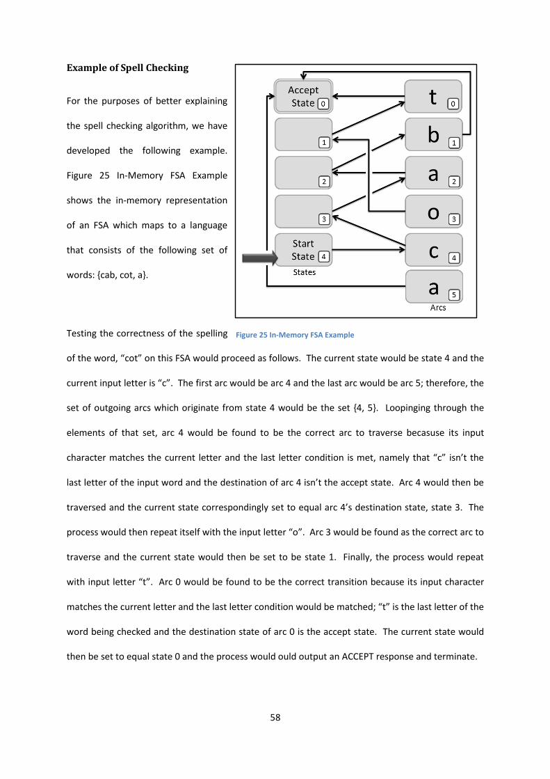
58
Example of Spell Checking
For the purposes of better explaining
the spell checking algorithm, we have
developed the following example.
Figure 25 In-Memory FSA Example
shows the in-memory representation
of an FSA which maps to a language
that consists of the following set of
words: {cab, cot, a}.
Testing the correctness of the spelling
of the word, “cot” on this FSA would proceed as follows. The current state would be state 4 and the
current input letter is “c”. The first arc would be arc 4 and the last arc would be arc 5; therefore, the
set of outgoing arcs which originate from state 4 would be the set {4, 5}. Loopinging through the
elements of that set, arc 4 would be found to be the correct arc to traverse becasuse its input
character matches the current letter and the last letter condition is met, namely that “c” isn’t the
last letter of the input word and the destination of arc 4 isn’t the accept state. Arc 4 would then be
traversed and the current state correspondingly set to equal arc 4’s destination state, state 3. The
process would then repeat itself with the input letter “o”. Arc 3 would be found as the correct arc to
traverse and the current state would then be set to be state 1. Finally, the process would repeat
with input letter “t”. Arc 0 would be found to be the correct transition because its input character
matches the current letter and the last letter condition would be matched; “t” is the last letter of the
word being checked and the destination state of arc 0 is the accept state. The current state would
then be set to equal state 0 and the process would ould output an ACCEPT response and terminate.
Figure 25 In-Memory FSA Example
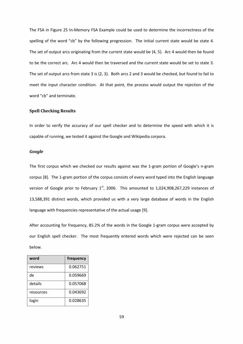
59
The FSA in Figure 25 In-Memory FSA Example could be used to determine the incorrectness of the
spelling of the word “cb” by the following progression. The initial current state would be state 4.
The set of output arcs originating from the current state would be {4, 5}. Arc 4 would then be found
to be the correct arc. Arc 4 would then be traversed and the current state would be set to state 3.
The set of output arcs from state 3 is {2, 3}. Both arcs 2 and 3 would be checked, but found to fail to
meet the input character condition. At that point, the process would output the rejection of the
word “cb” and terminate.
Spell Checking Results
In order to verify the accuracy of our spell checker and to determine the speed with which it is
capable of running, we tested it against the Google and Wikipedia corpora.
The first corpus which we checked our results against was the 1-gram portion of Google’s n-gram
corpus [8]. The 1-gram portion of the corpus consists of every word typed into the English language
version of Google prior to February 1st, 2006. This amounted to 1,024,908,267,229 instances of
13,588,391 distinct words, which provided us with a very large database of words in the English
language with frequencies representative of the actual usage [9].
After accounting for frequency, 85.2% of the words in the Google 1-gram corpus were accepted by
our English spell checker. The most frequently entered words which were rejected can be seen
below.
word frequency
reviews 0.062751
de 0.059669
details 0.057068
resources 0.043692
login 0.028635

60
reports 0.023037
rss 0.022574
sep 0.021198
ange 0.020102
records 0.019647
centre 0.019604
et 0.01759
al 0.015133
eur 0.015121
usr 0.014901
pre 0.014099
returns 0.014052
cnet 0.01349
mp3 0.012594
eg 0.012494
cities 0.012141
pdf 0.011785
programme 0.011648
ip 0.011542
los 0.010519
ie 0.009933
prev 0.009782
1st 0.00974
usb 0.009702
increased 0.00944
msn 0.009386
phentermine 0.009305
proposed 0.009213
described 0.009163
requires 0.008805
angeles 0.00866
releases 0.008461
units 0.00844

61
php 0.008322
zealand 0.008228
llc 0.008157
dvds 0.008116
texas 0.007714
las 0.007293
th 0.006988
detailed 0.006889
el 0.00683
dev 0.00681
returned 0.006691
shopping.com 0.006506
www 0.006501
tripadvisor 0.0065
pubmed 0.006394
xp 0.006376
xbox 0.006321
hong 0.00631
amazon.co.uk 0.006298
hentai 0.006294
asian 0.006292
milf 0.006272
devices 0.006231
au 0.006117
cds 0.006096
range 0.006029
usd 0.006018
multi 0.005889
di 0.005761
devel 0.005654
provisions 0.005636
sitemap 0.005622
username 0.005577
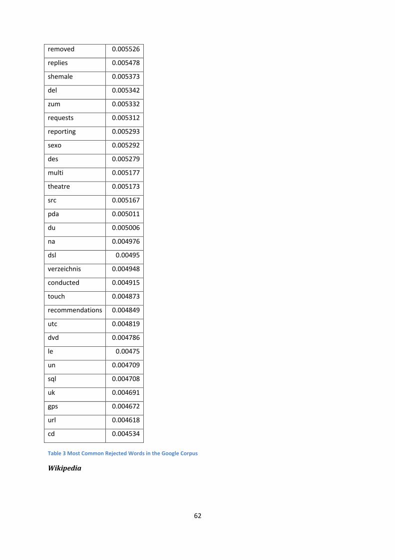
62
removed 0.005526
replies 0.005478
shemale 0.005373
del 0.005342
zum 0.005332
requests 0.005312
reporting 0.005293
sexo 0.005292
des 0.005279
multi 0.005177
theatre 0.005173
src 0.005167
pda 0.005011
du 0.005006
na 0.004976
dsl 0.00495
verzeichnis 0.004948
conducted 0.004915
touch 0.004873
recommendations 0.004849
utc 0.004819
dvd 0.004786
le 0.00475
un 0.004709
sql 0.004708
uk 0.004691
gps 0.004672
url 0.004618
cd 0.004534
Table 3 Most Common Rejected Words in the Google Corpus
Wikipedia
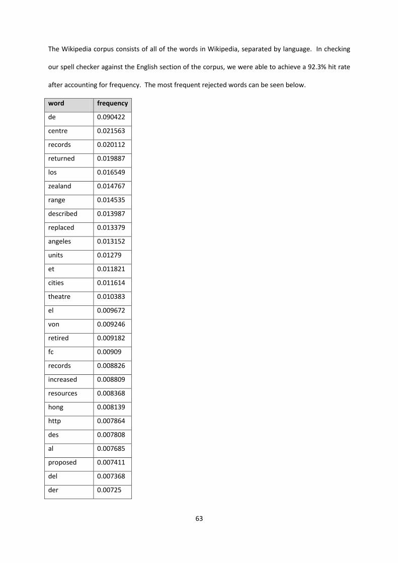
63
The Wikipedia corpus consists of all of the words in Wikipedia, separated by language. In checking
our spell checker against the English section of the corpus, we were able to achieve a 92.3% hit rate
after accounting for frequency. The most frequent rejected words can be seen below.
word frequency
de 0.090422
centre 0.021563
records 0.020112
returned 0.019887
los 0.016549
zealand 0.014767
range 0.014535
described 0.013987
replaced 0.013379
angeles 0.013152
units 0.01279
et 0.011821
cities 0.011614
theatre 0.010383
el 0.009672
von 0.009246
retired 0.009182
fc 0.00909
records 0.008826
increased 0.008809
resources 0.008368
hong 0.008139
http 0.007864
des 0.007808
al 0.007685
proposed 0.007411
del 0.007368
der 0.00725

64
voivodeship 0.00725
renamed 0.007126
removed 0.006997
labour 0.006775
du 0.006717
ret 0.00624
conducted 0.005981
defence 0.005945
gmina 0.005926
bgcolor 0.005889
details 0.005733
reports 0.005706
metres 0.005686
theatre 0.005566
sri 0.005552
refused 0.00537
di 0.005246
derived 0.005161
puerto 0.005117
ep 0.004685
returning 0.004669
programme 0.004658
didn 0.00465
prix 0.004594
und 0.004563
describes 0.004353
da 0.004145
las 0.004105
requires 0.003834
designs 0.003799
residing 0.003796
reviews 0.003778
returns 0.003684

65
capita 0.00368
devices 0.003641
rowspan 0.003624
releases 0.003562
restored 0.003448
cdp 0.003378
depending 0.003354
pts 0.003348
doesn 0.003325
organisation 0.003112
lanka 0.003077
detailed 0.003
iucn 0.002953
uefa 0.00292
br 0.002893
afterwards 0.00289
dnp 0.002885
range 0.00281
fifa 0.002809
anime 0.002729
costa 0.002699
sox 0.002662
replacing 0.002641
le 0.002568
colour 0.002565
scotia 0.00256
manga 0.002523
injuries 0.002521
colspan 0.002512
honours 0.002478
honour 0.002459
pos 0.002385
pdf 0.002375

66
friedrich 0.002372
recovered 0.002363
petersburg 0.002353
tons 0.002351
sr 0.002331
increases 0.00233
Table 4 Most Common Rejected Words in the English Wikipedia Corpus
Reasons for Rejects by the Spell Checker
While 85.2% and 92.3% hit rates may seem rather unimpressive, there were a variety of
circumstances under which it was desirable of our spell checker to reject a given word. Some of
these reasons are actual spelling errors, non-English words, highly technical terms that don’t belong
in a standard dictionary, and nonstandard abbreviations. The only problematic reason for rejecting
words is that our current finite state machine representations of languages were generated directly
from the aff / dic files and consequently only contain the word from those files. A future research
goal for the continuation of this project is to have linguists amend the RFSAs to include a broader
range of terms by using our spell checker to identify commonly used words that are being missed.
Chapter 3: Stemming
Stemming is an important task in natural language processing for a number of reasons. The most
common use of stemming is as a pre-processing step in information retrieval systems. For example,
a query containing a singular noun should return results containing the pluralized form of that noun
even if the singular version is absent [10]. This has historically been accomplished by comparing the
stems of the words in the query to the stems of the words in the document [11]. The more
accurately the stemming program can identify the roots, the higher the probability of matching
useful answers with the queries. This is especially true in smaller documents, which are less likely to
contain the same form of the word that was present in the query [10].

67
There are two types of suffixes which can be appended to stems, inflectional and derivational.
Inflectional suffixes are those which pluralize a word or change its tense. The inclusion or exclusion
of an inflectional suffix very rarely affects the meaning of the word. As such, it is always desirable
for a stemmer to remove such suffixes. Derivational suffixes are those which change the syntactic
category of the root word, i.e. changing a verb to a noun. Derivational suffixes are much more likely
to change the meaning of a word than inflectional suffixes and thus more care must be taken in
deciding when it is appropriate for them to be stripped [12].
History of Stemming
The Porter Stemmer
The Porter Stemmer has been one of the most prevalent stemmers since its conception. It was
designed as a rule-based stemmer. As such, it does not require an accompanying lexicon from which
to identify stems. The Porter Stemmer algorithm consists of a list of rules describing when suffixes
can be stripped from the input word. The longest suffix which can be stripped is stripped and this
process is iteratively repeated until there are no longer any suffixes which can be stripped [11]. The
Porter Stemmer was largely a success for its speed, ease of implementation in a variety of languages,
and relatively good performance when used in information retrieval [10].
Shortcomings of the Porter Stemmer
As the Porter Stemmer was created to be completely independent from a lexicon, it was forced to
suffer from several errors of both commission and omission.
Errors of Commission Errors of Omission
organization / organ european / europe
doing / doe analysis / analyzes
generalization / generic cylinder / cylindrical

68
numerical / numerous matrices / matrix
policy / police urgency / urgent
university / universe create / creation
easy / easily decompose / decomposition
addition / additive machine / machinery
negligible / negligent useful / usefully
execute / executive noise / noisy
define / definite route / routed
past / paste search / searcher
ignore / ignorant explain / explanation
arm / army resolve / resolution
head / heading triangle / triangular
[12]
For specific tasks, the Porter Stemmer suffered from an additional shortcoming other than over
conflation and narrow coverage. The stems returned by the Porter Stemmer would often not be
words in and of themselves [12]. While this was an acceptable occurrence for information retrieval,
it is unacceptable in linguistics based tasks which aim to actually identify root words.
Lexicon – Based Stemmers
Krovetz attempted to improve on the Porter Stemmer by using it in conjunction with a lexicon. His
method consisted of following the Porter algorithm with the additional step of checking if the word
is in the dictionary at each iteration. If it was in the dictionary, stripping ended. While this idea
initially looked promising, it ultimately failed. There are many words which strip off their last letter
before adding some suffixes and don’t for other suffixes. For such words there will be two disjoint

69
classes of suffixed forms and they will not be matched to each other. In English, the most common
occurrence of this is in words which end in the letter “e” [12].
After an early failure, Krovetz managed to surpass the Porter Stemmer by re-writing the rules to
output actual root words instead of just stems and hand-checking for the exceptions that had caused
errors for his modified version of the Porter algorithm. Most notably, he was very careful when
dealing with the suffixes “ed” and “es” about whether to strip one or two letters [12].
It is also possible to have a fully lexicon based stemmer. Since many dictionaries list root words and
the various suffixes which can be appended to them, the input words can just be matched against
this list and the appropriate stem returned. Unfortunately, this method, while accurate, is inefficient
to the point of being unusable.
Finite State Transducers in Stemming
The inefficiency problem of lexicon base transducers can be ameliorated by storing the lexicon in a
data structure which is more easily traversable. A finite state transducer is perfectly situated for this
task. Kokenniemi developed a small scale version of such an FST in hopes of it being later used to aid
in morphological analysis. However, he was never able to implement his architecture on a full
language and consequently wasn’t able to use the theories he developed in a meaningful way.
Additionally, his work was proprietary, belonging to Xerox, and thus unavailable to other researchers
to further develop [13].
Our Contribution to Open Source Stemming
We created a transducer based FST and an accompanying program in C which actually stems the
input words. This consisted of revising the compiler that we had created previously for spelling and
revising the spell checking program to appropriately handle output strings. As we can automatically
generate our FSTs from affix and dictionary files, we are able to support not only one real language,
but any real language for which aff / dic files have already been created.

70
Overall Stemming Process
We designed the
stemming process to be
very similar to the spell
checking process,
building on what we
created in the spell
checking compiler and
spell checking program
and adding the necessary
components to allow for
determining the root of a
word in addition to determining if the word had been spelled correctly. The main adjustment that
this required was for us to transform the C spell program into a stem program, i.e. handle output.
The minor components that we added were a printRoots() method in the Bison code and a
buildRoots() method in the C stemming program.
Extension of the Compiler to Support Stemming
In order to extend the compiler which we had previously created to support stemming, we merely
had to include pointers to an output string for each arc and store the output strings in an efficient
manner.
In-Memory Data Structures
We had to make one minor change to the RFSA data structure in order to transform it to an RFST
(Residual Finite State Transducer), namely to associate an output string with each arc in addition to
the input character that was already associated with each arc. This allowed us to generate output
Figure 26 Overall Stemming Process

71
from the input words. Additionally, we needed to design a data structure which could hold all of the
possible stems.
Stem List
We initially considered many options when deciding how
best to store the list of stems (output strings). The first
solution which we looked at can be viewed as the naïve
solution. It consisted of simply storing a list of words. The
arcs would then have pointers to the first character of the
corresponding word. This option had the obvious benefits
of ease of implementation and speed of determining the
output string associated with a given arc. However, it
suffered tremendously from the large amount of storage
required to contain such a list. We saw much of this
storage as wasted space and wanted to improve upon it.
As can be seen in Figure 27 Output Strings - Naive
SolutionError! Reference source not found., the letters at
the beginning of a word will be listed many times in such
an encoding scheme, even though it is clearly visible that
in such an alphabetical listing, all of the words between
the first word beginning with an “a” and the first word
beginning with a “b” will begin with an “a.” Likewise, all
of the words between the first words beginning with the
characters: and the first word beginning with the
characters will begin with the characters
. The naïve solution allots space for every character of every output string, and thus
Figure 27 Output Strings - Naive Solution

72
consumes as much space as could ever reasonably be allotted. However, as was shown above, much
of this space is clearly unnecessary.
That finding motivated us to investigate the use of a trie based solution to the stem storage
problem. Figure 28 Output Strings - Trie Based Solution shows the tree based solution for the same
set of root words that was used in the naïve solution above. At first glance, this solution seems to be
much better, as the fewest possible number of characters is used. However, the most significant
benefit of the naïve solution, the ease of output string determination, has been completely reversed.
In this case, determining the output string requires a very messy traversal of pointers. The arc will
have to point to the last letter of the word in order for there to exist a deterministic way of
identifying the input string. However, it is very difficult to determine the state which came before a
given state; being able to do so would have required us to store pointers between all of the nodes in
the trie in addition to storing the nodes themselves. By that point, we would have lost all of the
benefits gained from storing as few characters as possible.

73
We eventually decided to implement a hybrid of the previous two solutions. Most of the repetition
in characters can be found in the first few characters of a word. For a given 2 letter sequence, there
Figure 28 Output Strings - Trie Based Solution

74
are generally going to
be many words which
begin with that
sequence. However,
for a 5 letter
sequence, there are
going to be very few
words which begin
with that sequence.
We chose to set the
cutoff tolerance for
the number of letters
at the beginning of a word to group by at 2. This decision was based primarily on intuition derived
from experience with language and was validated by the guidance of Kornai András.
Our hybrid approach consists of subdividing the output strings into classes corresponding to two-
letter strings. A word, w, is placed in the set if the first two letters of w are . The data
storage consists of a series of linked lists, one for each set. The first element of each linked list is the
two letter string associated with that set. The subsequent elements of the linked list are the strings
that can be appended to the two letter string to form valid output strings.
Overall, this data structure seemed to meet all of our needs. The only things which it was ill-
equipped to handle were one and two letter output strings. The problem of two letter output
strings was easily circumvented by allowing arcs to point to the first element of the linked list. Single
letter output strings were more complicated, because they weren’t encoded for anywhere in the
current data structure. In order to handle this, we allow there to be a separate linked list consisting
of single character elements.
Figure 29 Output Strings - Hybrid Solution
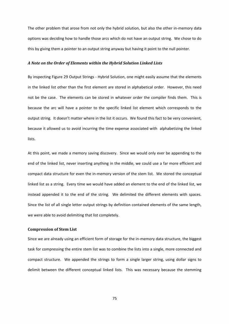
75
The other problem that arose from not only the hybrid solution, but also the other in-memory data
options was deciding how to handle those arcs which do not have an output string. We chose to do
this by giving them a pointer to an output string anyway but having it point to the null pointer.
A Note on the Order of Elements within the Hybrid Solution Linked Lists
By inspecting Figure 29 Output Strings - Hybrid Solution, one might easily assume that the elements
in the linked list other than the first element are stored in alphabetical order. However, this need
not be the case. The elements can be stored in whatever order the compiler finds them. This is
because the arc will have a pointer to the specific linked list element which corresponds to the
output string. It doesn’t matter where in the list it occurs. We found this fact to be very convenient,
because it allowed us to avoid incurring the time expense associated with alphabetizing the linked
lists.
At this point, we made a memory saving discovery. Since we would only ever be appending to the
end of the linked list, never inserting anything in the middle, we could use a far more efficient and
compact data structure for even the in-memory version of the stem list. We stored the conceptual
linked list as a string. Every time we would have added an element to the end of the linked list, we
instead appended it to the end of the string. We delimited the different elements with spaces.
Since the list of all single letter output strings by definition contained elements of the same length,
we were able to avoid delimiting that list completely.
Compression of Stem List
Since we are already using an efficient form of storage for the in-memory data structure, the biggest
task for compressing the entire stem list was to combine the lists into a single, more connected and
compact structure. We appended the strings to form a single larger string, using dollar signs to
delimit between the different conceptual linked lists. This was necessary because the stemming

76
program must be able to determine the two letter word beginning of the output string in addition to
the rest of the string.
We then had to handle adding the linked list of single character elements into our agglutenated
string. We did this by inserting dollar signs before every character in the string representation of
that list and then appending the string corresponding to the rest of the linked lists to the end of the
string for the single characters. An example end product of this process can be seen in Figure 31
Compressed Stems with Single Letter Stems.
Figure 30 Compressed Stems
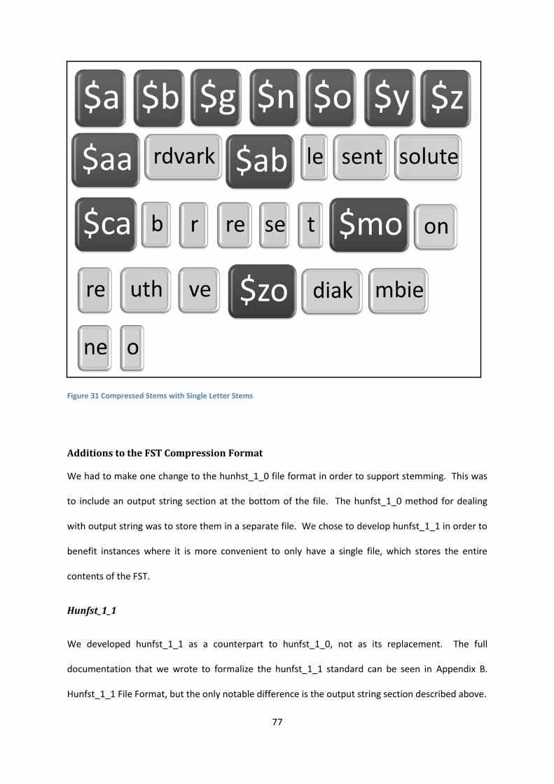
77
Additions to the FST Compression Format
We had to make one change to the hunhst_1_0 file format in order to support stemming. This was
to include an output string section at the bottom of the file. The hunfst_1_0 method for dealing
with output string was to store them in a separate file. We chose to develop hunfst_1_1 in order to
benefit instances where it is more convenient to only have a single file, which stores the entire
contents of the FST.
Hunfst_1_1
We developed hunfst_1_1 as a counterpart to hunfst_1_0, not as its replacement. The full
documentation that we wrote to formalize the hunfst_1_1 standard can be seen in Appendix B.
Hunfst_1_1 File Format, but the only notable difference is the output string section described above.
Figure 31 Compressed Stems with Single Letter Stems
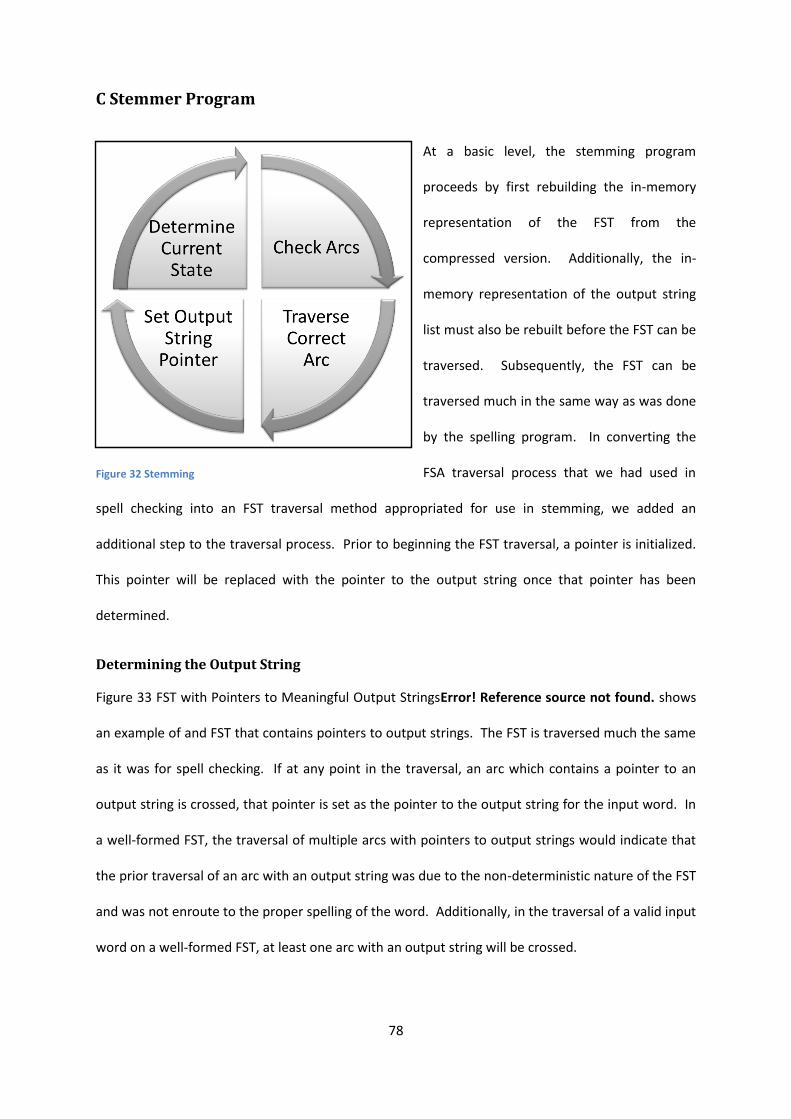
78
C Stemmer Program
At a basic level, the stemming program
proceeds by first rebuilding the in-memory
representation of the FST from the
compressed version. Additionally, the in-
memory representation of the output string
list must also be rebuilt before the FST can be
traversed. Subsequently, the FST can be
traversed much in the same way as was done
by the spelling program. In converting the
FSA traversal process that we had used in
spell checking into an FST traversal method appropriated for use in stemming, we added an
additional step to the traversal process. Prior to beginning the FST traversal, a pointer is initialized.
This pointer will be replaced with the pointer to the output string once that pointer has been
determined.
Determining the Output String
Figure 33 FST with Pointers to Meaningful Output StringsError! Reference source not found. shows
an example of and FST that contains pointers to output strings. The FST is traversed much the same
as it was for spell checking. If at any point in the traversal, an arc which contains a pointer to an
output string is crossed, that pointer is set as the pointer to the output string for the input word. In
a well-formed FST, the traversal of multiple arcs with pointers to output strings would indicate that
the prior traversal of an arc with an output string was due to the non-deterministic nature of the FST
and was not enroute to the proper spelling of the word. Additionally, in the traversal of a valid input
word on a well-formed FST, at least one arc with an output string will be crossed.
Figure 32 Stemming

79
This process has been made slightly more complex because arcs which we would not normally want
to have output strings at all have been designed to instead have pointers to NULL as their output
string. In this situation, every arc has an output string and thus the pointer to the output string of
the input word would have been changed at every arc traversal under the aforementioned traversal
algorithm. As such, any suffixed words would be set to have NULL as their stem, even though this is
not accurate. What this means is that during traversal, a previous pointer to an output string is only
replaced if the replacement doesn’t point to NULL.
Figure 33 FST with Pointers to Meaningful Output Strings

80
Figure 35 Indexed Stem List shows the pointers to the list of input words. Once the pointer for an
output string has been found the actual output string is determined as follows. The output string is
initially set to equal the word pointed to. If this word begins with a dollar sign, the dollar sign is
stripped and the algorithm terminates. Otherwise, the list is traversed backwards until a dollar sign
Figure 34 FST with Output String Pointers for All Arcs
Figure 35 Indexed Stem List

81
is encountered. The two letters following the dollar sign are then appended to the beginning of the
output word and the algorithm then terminates.
Chapter 4: Future Research
For future research, we would love to see the finite state transducer model that we have given to
the open source community extended to support morphological analysis. This would be relatively
simple, as the morphDB versions of the aff / dic files contain morphological annotations. The
shortcoming of this would be that morphDB is available for very few languages. However, morphDB
formats are being developed for more languages and the development of an advanced tool such as a
morphological analyzer which supports morphDB might help to increase motivation to speed up the
process.
Additionally, we would like to see linguistic research efforts put forth towards improving the
available aff / dic files. We found most of our shortcomings to stem from missing entries in the aff /
dic files. It would be very interesting for us to see how much better coverage we could obtain if
given better input files.

82
References
1. Computer Programs for Detecting and Correcting Spelling Errors. Peterson, James, L. s.l. :
Association for Computing Machinery, December 1980, Communications of the ACM, Vol. 23, pp.
676-687.
2. Kuenning, Geoff. Where it came from. XEmacs. [Online] October 2007. [Cited: April 13, 2010.]
http://www.xemacs.neoscientists.org/Documentation/packages/html/ispell_6.html.
3. —. International Ispell. Laboratory for Advanced Systems Research. [Online] 3.3.02,07, June 7,
2001. [Cited: April 6, 2010.] http://www.lasr.cs.ucla.edu/geoff/ispell.html.
4. —. International Ispell. Laboratory for Advanced Systems Research. [Online] April 1996. [Cited:
April 13, 2010.] http://www.lasr.cs.ucla.edu/geoff/ispell.html.
5. Németh, László, et al., et al. Open Source Morphological Analyzer. [CD-ROM] 1.0, Philadelphia,
Pennsylvania, United States of Ameriaca : Linguistic Data Consortium, 2008. Hungarian-English
Parallel Text.
6. Karttunen, Lauri and Beesley, Kenneth R. Twenty-Five Years of Finite-State Morphology. Inquiries
Into Words, a Festschrift for Kimmo Koskenniemi on his 60th Birthday. Stanford : CSLI Studies in
Computational Linguistics, 2005, pp. 72-83.
7. The Flex Project. Flex: The Fast Lexical Analyzer. [Online] 2008. [Cited: April 15, 2010.]
http://flex.sourceforge.net/.
8. Free Software Foundation. Bison - GNU parser generator. GNU Operating System. [Online] May 1,
2009. [Cited: April 15, 2010.] http://www.gnu.org/software/bison/.

83
9. Németh, László. Hunspell. sourceforge. [Online] 1.2.9. [Cited: April 12, 2010.]
http://hunspell.sourceforge.net/.

84
Appendices
Appendix A. Hunfst_1_0 File Format
File Format for hunfst_1_0
Sections of the File==============================================================
# may be used at the beginning of a line anywhere within the file to denote that that line should be
ignored by the compiler
@scheme <digit> <string>
It is necessary that all arcs include 1 or 2 bytes devoted to the input character; most languages will
only require 1 byte for this, but languages with many distinct characters such as Chinese and
Japanese will require 2. Each arc also requires a 3 byte pointer to the output state. The exact
number of bytes devoted to this is dependent on the total number of states. An optional 3 bytes can
be used as a pointer to an output string if a transducer, not and automata, is being described. If this
is being done, a table of output strings must be stored somewhere. This output string can, in
addition to simply listing the output value of the transducer, also include elements such as part of
speech tags. An optional 1-4 bytes may be used to give a probability value to each arc. It is not
necessary to devote any space in this structure to define whether or not a given state is a final state,
because the first state(s) listed will always be the only final state(s) in the transducer.
The digit is the number of bytes per arc. Valid values are integers between 4 and 12, inclusive.
The string is the name of the scheme being implemented by this transducer's arcs. An external file
will contain the list of all scheme names and their corresponding descriptions.
@lang <aa_bb>
aa is the 2 letter language code. bb is the 2 letter country code.

85
@charset <string>
The string is the name of the encoding used by the language being described.
@internal-charset <string>
The string is the name of the encoding used within the hunfst file itself. In general, this will be the
same as the charset used by the language or some superset thereof. This is because it is necessary
to be able to write all of the possible input characters.
@states <number>
This number is the total number of states.
This is the beginning of the states sections. At this point, there will be a line containing a list of
unique states. Each state will consist of a pointer to the first arc which originates from that state.
Since the number of bytes in each pointer is known ahead of time, it is not necessary to waste any
memory with delimiters between states. The contents of each state are written byte by byte in
hexadecimal notation.
@arcs <number>
The number is equal to the number of arcs.
This is the beginning of the arcs section. One line is devoted to each arc. The contents of each arc
are written bitwise in hexadecimal notation and the meaning of the byte is as was described above.
@cksum <number>
The check sum value is used to ensure that there were no errors incurred while copying or moving
the file.

86
Appendix B. Hunfst_1_1 File Format
hunfst_1_1 is a variant on hunfst_1_0 that has been specially designed to handle finite state
transducer models of languages for stemming. In this version of hunfst, output pointers are a
necessary component of all arcs. In the case where there shouldn’t be an output pointer associated
with a given arc, the pointer consisting of all nines (in decimal notation) is used as a place holder.
hunfst_1_1 introduces an additional section which lists the output strigs.
File Format for hunfst_1_0
Sections of the File==============================================================
# may be used at the beginning of a line anywhere within the file to denote that that line should be
ignored by the compiler
@scheme <digit> <string>
It is necessary that all arcs include 1 or 2 bytes devoted to the input character; most languages will
only require 1 byte for this, but languages with many distinct characters such as Chinese and
Japanese will require 2. Each arc also requires a 3 byte pointer to the output state. The exact
number of bytes devoted to this is dependent on the total number of states. An optional 3 bytes can
be used as a pointer to an output string if a transducer, not and automata, is being described. If this
is being done, a table of output strings must be stored somewhere. This output string can, in
addition to simply listing the output value of the transducer, also include elements such as part of
speech tags. An optional 1-4 bytes may be used to give a probability value to each arc. It is not
necessary to devote any space in this structure to define whether or not a given state is a final state,
because the first state(s) listed will always be the only final state(s) in the transducer.
The digit is the number of bytes per arc. Valid values are integers between 4 and 12, inclusive.
The string is the name of the scheme being implemented by this transducer's arcs. An external file
will contain the list of all scheme names and their corresponding descriptions.

87
@lang <aa_bb>
aa is the 2 letter language code. bb is the 2 letter country code.
@charset <string>
The string is the name of the encoding used by the language being described.
@internal-charset <string>
The string is the name of the encoding used within the hunfst file itself. In general, this will be the
same as the charset used by the language or some superset thereof. This is because it is necessary
to be able to write all of the possible input characters.
@states <number>
This number is the total number of states.
This is the beginning of the states sections. At this point, there will be a line containing a list of
unique states. Each state will consist of a pointer to the first arc which originates from that state.
Since the number of bytes in each pointer is known ahead of time, it is not necessary to waste any
memory with delimiters between states. The contents of each state are written byte by byte in
hexadecimal notation.
@arcs <number>
The number is equal to the number of arcs.
This is the beginning of the arcs section. One line is devoted to each arc. The contents of each arc
are written bitwise in hexadecimal notation and the meaning of the byte is as was described above.
@output
The output section consists exclusively of a compressed list of root words. The compression has
been designed to adhere to the following standard. Root words are divided into two sections, the
first being their first two letters, and the second being the rest of the word. The encoding scheme

88
for a single two letter word beginning consists of “$” followed by a two letter word beginning,
followed by all possible word endings that can match that word beginning. The different word parts
are delimited by spaces. Such an encoding is written for each two letter word beginning.
@cksum <number>
The check sum value is used to ensure that there were no errors incurred while copying or moving
the file.
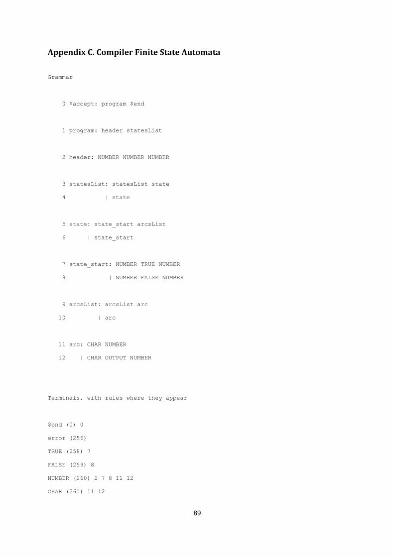
89
Appendix C. Compiler Finite State Automata
Grammar
0 $accept: program $end
1 program: header statesList
2 header: NUMBER NUMBER NUMBER
3 statesList: statesList state
4 | state
5 state: state_start arcsList
6 | state_start
7 state_start: NUMBER TRUE NUMBER
8 | NUMBER FALSE NUMBER
9 arcsList: arcsList arc
10 | arc
11 arc: CHAR NUMBER
12 | CHAR OUTPUT NUMBER
Terminals, with rules where they appear
$end (0) 0
error (256)
TRUE (258) 7
FALSE (259) 8
NUMBER (260) 2 7 8 11 12
CHAR (261) 11 12

90
OUTPUT (262) 12
Nonterminals, with rules where they appear
$accept (8)
on left: 0
program (9)
on left: 1, on right: 0
header (10)
on left: 2, on right: 1
statesList (11)
on left: 3 4, on right: 1 3
state (12)
on left: 5 6, on right: 3 4
state_start (13)
on left: 7 8, on right: 5 6
arcsList (14)
on left: 9 10, on right: 5 9
arc (15)
on left: 11 12, on right: 9 10
state 0
0 $accept: . program $end
NUMBER shift, and go to state 1
program go to state 2
header go to state 3
state 1

91
2 header: NUMBER . NUMBER NUMBER
NUMBER shift, and go to state 4
state 2
0 $accept: program . $end
$end shift, and go to state 5
state 3
1 program: header . statesList
NUMBER shift, and go to state 6
statesList go to state 7
state go to state 8
state_start go to state 9
state 4
2 header: NUMBER NUMBER . NUMBER
NUMBER shift, and go to state 10
state 5
0 $accept: program $end .

92
$default accept
state 6
7 state_start: NUMBER . TRUE NUMBER
8 | NUMBER . FALSE NUMBER
TRUE shift, and go to state 11
FALSE shift, and go to state 12
state 7
1 program: header statesList .
3 statesList: statesList . state
NUMBER shift, and go to state 6
$default reduce using rule 1 (program)
state go to state 13
state_start go to state 9
state 8
4 statesList: state .
$default reduce using rule 4 (statesList)
state 9

93
5 state: state_start . arcsList
6 | state_start .
CHAR shift, and go to state 14
$default reduce using rule 6 (state)
arcsList go to state 15
arc go to state 16
state 10
2 header: NUMBER NUMBER NUMBER .
$default reduce using rule 2 (header)
state 11
7 state_start: NUMBER TRUE . NUMBER
NUMBER shift, and go to state 17
state 12
8 state_start: NUMBER FALSE . NUMBER
NUMBER shift, and go to state 18
state 13
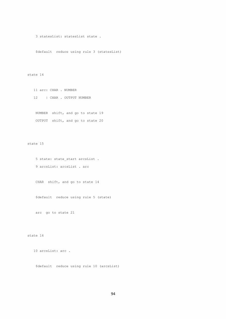
94
3 statesList: statesList state .
$default reduce using rule 3 (statesList)
state 14
11 arc: CHAR . NUMBER
12 | CHAR . OUTPUT NUMBER
NUMBER shift, and go to state 19
OUTPUT shift, and go to state 20
state 15
5 state: state_start arcsList .
9 arcsList: arcsList . arc
CHAR shift, and go to state 14
$default reduce using rule 5 (state)
arc go to state 21
state 16
10 arcsList: arc .
$default reduce using rule 10 (arcsList)

95
state 17
7 state_start: NUMBER TRUE NUMBER .
$default reduce using rule 7 (state_start)
state 18
8 state_start: NUMBER FALSE NUMBER .
$default reduce using rule 8 (state_start)
state 19
11 arc: CHAR NUMBER .
$default reduce using rule 11 (arc)
state 20
12 arc: CHAR OUTPUT . NUMBER
NUMBER shift, and go to state 22
state 21
9 arcsList: arcsList arc .
$default reduce using rule 9 (arcsList)

96
state 22
12 arc: CHAR OUTPUT NUMBER .
$default reduce using rule 12 (arc)
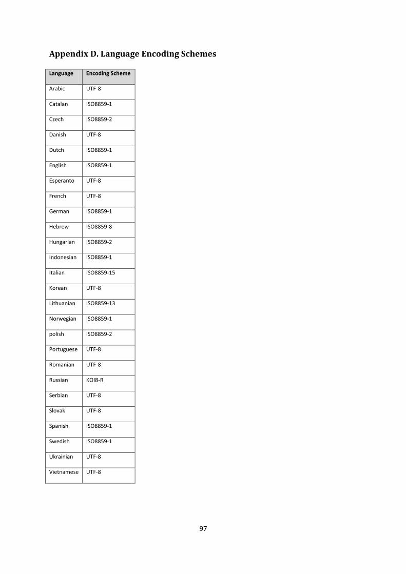
97
Appendix D. Language Encoding Schemes
Language Encoding Scheme
Arabic UTF-8
Catalan ISO8859-1
Czech ISO8859-2
Danish UTF-8
Dutch ISO8859-1
English ISO8859-1
Esperanto UTF-8
French UTF-8
German ISO8859-1
Hebrew ISO8859-8
Hungarian ISO8859-2
Indonesian ISO8859-1
Italian ISO8859-15
Korean UTF-8
Lithuanian ISO8859-13
Norwegian ISO8859-1
polish ISO8859-2
Portuguese UTF-8
Romanian UTF-8
Russian KOI8-R
Serbian UTF-8
Slovak UTF-8
Spanish ISO8859-1
Swedish ISO8859-1
Ukrainian UTF-8
Vietnamese UTF-8

98
Appendix E. Affix File Format
Standard:
Many keywords have overloaded meaning. In such cases the first time the keyword shows up for a
particular flag, it is to mark the number of rules following it containing that flag, or keyword. These
cases are have the Form: KEYWORD <number> line in the following documentation denoting that
the flag can take that form. Keywords that do not have a “Form:” descriptor are keywords that turn
on or off an option by existing in the file or not.
LANG is the keyword setting the language associated with this affix file
Form: LANG <language>
SET is the he character encoding set used with this language
TRY is the set of characters in order from most to least frequently used.
Example (from English) TRY esianrtolcdugmphbyfvkwzESIANRTOLCDUGMPHBYFVKWZ'
FLAG is the Affix flag type.
The following options will follow this keyword:
default is the ascii
UTF is the flags will be using UTFis the8 characters

99
long is the flags will be 2 ASCII characters long
num is the flags are marked
Form: FLAG <option>
COMPLEXPREFIXES is the keyword that allows for twofold suffix stripping (see linguistics basics)
NOSUGGEST marks a word that may be a word in the dictionary, but should not be suggested as a
possible correct spelling for a misspelled word. This is used to mark vulgar words.
MAXNGRAMSUGS sets the maximum Lowenstein distance between the suggested word’s spelling
and the mispelled word’s spelling.
NOSPLITSUGS is a keyword disabling suggestions that are actually two separate words.
SUGSWITHDOTS is the If this keyword is present in the affix file, add a dot to the end of the word in
suggestions if there was a dot at the end of the original word. For example, if the word read Mf., the
keyword SUGSWITHDOTS would offer Mr. as a suggestion. This keyword does not work in Open
Office, because Open Office already has this functionality.
MAP maps a letter that is commonly mistaken for another letter to that letter for use in suggestions.

100
COMPOUNDMIN sets the length of the shortest possible word to consider compounding. Without
this keyword, the default is 3.
Form: COMPOUNDMIN <number>.
COMPOUNDFLAG sets the flag that marks a word available to be compounded
Form: COMPOUNDFLAG <flag>
COMPOUNDBEGIN sets the flag that allows a word first part of a compound word
Form: COMPOUNDBEGIN <flag>
COMPOUNDMIDDLE sets the flag that allows a word to be in the middle of a compound word
Form: COMPOUNDBEGIN <flag>
ONLYINCOMPOUND is the marks a suffix that can only be found inside a compound word
Form: ONLYINCOMPOUND <flag>
COMPOUNDPERMITFLAG is the by default, prefixes are allowed in the beginning of compound
words, and suffixes go at the end. COMPOUNDPERMITFLAG allows prefixes and suffixes to also be
part of the words that are being compounded.

101
Form: COMPOUNDPERMITFLAG <flag>
COMPOUNDFORBIDFLAG sets the flag that assures that a version of a word that has had affixes
added will not be compounded
Form: COMPOUNDFORBIDFLAG <flag>
COMPOUNDROOT sets the flag that marks compounds that are in the dictionary
Form: COMPOUNDROOT <flag>
COMPOUNDWORDMAX is the By default, words can be compounded on each other infinitely. This
flag sets a maximum amount of words that can be in a compound word
Form: COMPOUNDWORDMAX <number>
CHECKCOMPOUNDDUP is the assures that words will not be duplicated in compound words. For
example, if foo is a word that can be compounded, this keyword would not allow the word foofoo
CHECKCOMPOUNDREP assures that if a compounded word could also be a misspelled word with
letter from REP in it, it doesn’t get marked spelled properly.
CHECKCOMPOUNDCASE assures that words within compound words are not allowed to have capital

102
letters
CHECKCOMPOUNDTRIPLE assures that words will not compound if it will create a word with a triple
letter run, such as bar|rro or foo|ox.
CHECKCOMPOUNDPATTERN forbids letters that end a word and letters that begin the next word of a
compound word from appearing together.
Form: CHECKCOMPOUNDPATTERN number_of_definition
Form: CHECKCOMPOUNDPATTERN end_chars begin_chars
COMPOUNDSYLLABLE makes sure that a word that has more words than COMPOUNDWORDMAX
have less syllables than the first parameter of this keyword. Syllables are calculated from the list of
vowels that make up the second parameter.
Form: COMPOUNDSYLLABLE <max_syllables> <list_of_vowels>
SYLLABLENUM “Needed for special rules in Hungarian [14]”
Form: Syllablenum <flags>
FORBIDDENWORD defines a flag denoting a word that cannot exist.
Form: FORBIDDENWORD <flag>

103
WORDCHARS defines characters that are acceptable as parts of single words. “For example, dot,
dash, n-dash, numbers, percent sign are word character in Hungarian.”
REP creates suggestions of characters to replace the characters they are commonly mistaken for. In
English an example may be REP ph f. It can also be used the same way for words.
Form: REP <number_of_definitions>
Form: REP original replacement
CIRCUMFIX defines the flag denoting that a word exists as long as it also has a prefix. In some
languages, such as German, the
KEEPCASE defines the flag denoting a word that is acceptable in lowercase form, but not uppercase
form.
From: KEEPCASE flag
LEMMA_PRESENT flag separating dictionary words that are real lemmas from dictionary words that
are actually affixed forms.
Form: LEMMA_PRESENT <flag>

104
NEEDAFFIX sets the flag denoting a word that cannot exist in a non-affixed form.
PSEUDOROOT is the former name of NEEDAFFIX. It has been deprecated.
COMPOUNDRULE defines a custom compound pattern using a regular expression-like syntax.
This keyword is not compatible with any other compound keywords, and as such should not be used
with any of them.
Form: COMPOUNDRULE <number_of_definitions>
Form: COMPOUNDRULE <pattern>
CHECKSHARPS is a keyword letting Hunspell know it should look for special cases of capitalized
letters. In German, for example when the letter-pair SS exists in a place that should be capitalized,
they are capitalized together as a “sharp S.”
COMPOUNDEND sets the flag that allows a word last part of a compound word
Form: COMPOUNDEND <flag>
BREAK denotes characters that can be the break points between compounded words. Break works
recursively.
Form: BREAK <number_of_break_definitions>

105
Form: BREAK <character_or_character_sequence_that_can_break_words>
KEY - a keyword marking letters that are close to each other on the keyboard. Here is a basic
example for a QWERTY keyboard: KEY qwertyuiop|asdfghjkl|zxcvbnm. It is also possible to mark
letters that are near each other by adding additional conditions. For example, the above example
could have included |kjm
ICONV - marks an input conversion table. This keyword assures that if a character can be written
two separate ways, both will be seen as correct.
Form: ICONV <number_of_conversions>
Form: ICONV <char> <char>
OCONV -does the same thing as ICONV for an output conversion table.
Form: ICONV <number_of_conversions>
Form: ICONV <char> <char>
AF substitutes cardinal numbers for affix flags
Form: AF number_of_flag_vector_aliases
Form: AF flag_vector

106
IGNORE lists the characters that can be ignored in a word. This is useful for languages such as Arabic
and Hebrew where diacritical marks are optional in a word
Form: IGNORE <characters>
SIMPLIFIEDTRIPLE is a keyword allowing compound words that would cause a triple letter to occur,
to strip one of those letters. This phenomena is found in correctly spelled Norwegian and Swedish
words.
SFX A keyword denoting a flag for a suffix that can be added to a word
SFX has the following options:
Cross-product - Y or N (yes or no) flag permitting prefix/suffix combinations
Stripping - defines letter or letters to be stripped from the end of the non-affixed form. If no
stripping will be necessary, the value of this flag is ‘0’
Suffix - character or characters to add to the end of a word
Condition - regular expression type character, string, or set of characters stating under what
conditions the suffix can be added
Condition Form: [chars...]denotes a set of single characters that must be present in order to apply
the SFX rule
^ denotes a character (or string) that cannot be present in order to apply the SFX rule
[^chars] denotes a set of characters that cannot be present in order to apply this rule

107
Morphological fields - ease morphological analysis of words. This tag is optional.
Form: SFX <flag> <cross_product> <number_of_rules_with_this_flag>
Form: SFX <flag> <stripping> <suffix> <condition> [morphological_fields...]
PFX A keyword denoting a flag for a prefix that can be added to a word
SFX has the following options:
Cross-product - Y or N (yes or no) flag permitting prefix/suffix combinations
Stripping - defines letter or letters to be stripped from the beginning of the non-affixed form. If no
stripping will be necessary, the value of this flag is ‘0’
Suffix - character or characters to add to the beginning of a word
Condition - regular expression type character, string, or set of characters stating under what
conditions the suffix can be added
Condition Form: [chars...]denotes a set of single characters that must be present in order to apply
the SFX rule
^ denotes a character (or string) that cannot be present in order to apply the SFX rule
[^chars] denotes a set of characters that cannot be present in order to apply this rule
Morphological fields - ease morphological analysis of words. This tag is optional.
Form: PFX <flag> <cross_product> <number_of_rules_with_this_flag>
Form: SFX <flag> <stripping> <suffix> <condition> [morphological_fields...]

108
(9)

109