WORKING PAPER SERIES

Open Market Operations and the Federal Funds Rate

Daniel L. Thornton

Working Paper 2005-063A http://research.stlouisfed.org/wp/2005/2005-063.pdf

September 2005

FEDERAL RESERVE BANK OF ST. LOUIS Research Division 411 Locust Street

St. Louis, MO 63102 ______________________________________________________________________________________

The views expressed are those of the individual authors and do not necessarily reflect official positions of the Federal Reserve Bank of St. Louis, the Federal Reserve System, or the Board of Governors.

Federal Reserve Bank of St. Louis Working Papers are preliminary materials circulated to stimulate discussion and critical comment. References in publications to Federal Reserve Bank of St. Louis Working Papers (other than an acknowledgment that the writer has had access to unpublished material) should be cleared with the author or authors.

Photo courtesy of The Gateway Arch, St. Louis, MO. www.gatewayarch.com

Open Market Operations and the Federal Funds Rate

Daniel L. Thornton Federal Reserve Bank of St. Louis

Phone (314) 444-8582 FAX (314) 444-8731

email Address: thornton@stls.frb.org

Abstract

It is commonly believed that the Fed’s ability to control the federal funds rate stems from its ability to alter the supply of liquidity in the overnight market through open market operations. This paper uses daily data compiled by the author from the records of the Trading Desk of the Federal Reserve Bank of New York over the period March 1, 1984, through December 31, 1996, to analyze the Desk’s use of its operating procedure in implementing monetary policy, and the extent to which open market operations affect the federal funds rate—the liquidity effect. I find that operating procedure was used to guide daily open market operations; however, there is little evidence of a liquidity effect at the daily frequency and even less evidence at lower frequencies. Consistent with the absence of a liquidity effect, open market operations appear to be a relatively unimportant source of liquidity to the federal funds market.

JEL Classification: E43, E52 Key Words: open market operations, federal funds rate, federal funds market, operating procedure, monetary policy The views expressed here are the author’s and do not necessarily reflect the views of the Board of Governors of the Federal Reserve System or the Federal Reserve Bank of St. Louis. I would like to thank John Partlan, and Sherry Edwards for many valuable comments and John McAdams for valuable research assistance.

1

1.0 Introduction

The conventional view is that the Fed controls the federal funds rate by altering

the supply of liquidity in the overnight market by changing the supply of reserves relative

to demand through open market operations (e.g., Taylor, 2001, Friedman, 1999). Open

market operations are conducted by the Trading Desk of the Federal Reserve Bank of

New York (the Desk). While the procedure that the Desk follows has evolved and

continues to do so, the fundamental procedure has remained largely the same since at

least the mid-to-late 1970s. Specifically, the Desk estimates (a) the demand for reserves

that are required to achieve the FOMC’s operating objective and (b) the quantity of

reserves that would be available if the Desk did nothing. If (a) exceeds (b), the procedure

indicates that reserves be added through an open market purchase of government

securities. If (a) is less than (b), the procedure suggests that the Desk drain reserves

through an open market sale.

It is important to note that the operating procedure is intended only to provide the

Desk with guidance in conducting daily open market operations. It was never intended to

be strictly adhered to. Specifically, frequent, yet informal, adjustments to the estimate of

excess reserves were made.1 Moreover, the Desk behavior is also guided by other

factors, such as its estimate of free reserves, in determining the day’s open market

operations.

This paper uses daily data compiled by the author from the records of the Trading

Desk of the Federal Reserve Bank of New York to analyze the effect of open market

1 These informal adjustments were stated in the morning call and depended upon estimates of the distribution of cumulative excess reserves holding to date. These informal adjustments were particularly important on the last two days of the maintenance period.

2

operations.2 The paper addresses two issues: the use of the operating procedure in

implementing monetary policy and the extent to which open market operations affect the

federal funds rate—the liquidity effect. In so doing, it provides some evidence on the

relative importance of Fed operations in supplying liquidity to the federal funds market.

Section 2 presents the Desk’s operating procedure in detail and analyzes the

Desk’s use of the procedure. Section 3 investigates the relationship between open market

operations and the federal funds rate. An analysis of these findings, as well as the

conclusions, is presented in Section 4.

2.0 The Desk’s Operating Procedure

The equilibrium federal funds rate is determined by the demand for and supply of

total reserves. Hence, the Desk’s operating procedure under a federal funds targeting

procedure is simply to equate the supply of reserves with the expected demand,

conditional on the target for the federal funds rate. To illustrate the procedure, assume

that the demand for total reserves ( ) is given by dTR

(1) ( , )dt t tTR f ff x tη= + ,

where tff is the federal funds rate, xt is a vector of other variables that determine reserve

demand, and tη is a random i.i.d. demand shock. Implicitly, the demand for reserves

includes the demand for excess reserves—reserves in excess of those needed to satisfy

Federal Reserve-imposed reserve requirements.

The quantity of total reserves supplied if the Desk conducts no open market

operations is determined by the Fed’s holding of government securities, Bt , borrowing by

2 The Federal Reserve Bank of New York and the Board of Governors of the Federal Reserve jointly control the access to and the use of these data. I would like to thank Jonathan Albrecht and Joanna Barnish for their valuable assistance in gathering these data and John Partlan for helping me understand the nuances of the Desk’s operating procedure.

3

depository institutions, BRt , and what the Desk refers to as autonomous factors that affect

reserve supply, Ft , e.g., currency in circulation, the Treasury’s balance at the Fed, the

float, etc.3 That is,

(2) . st t tTR B BR F= + + t

In practice, the Desk knows the magnitude of none of the variables on the right-hand-side

of (2) at the time that it conducts open market operations; however, because the errors are

very small for tB , for the sake of this analysis Bt is assumed to be known exactly.4 The

Desk makes an estimate of the autonomous factors that affect reserve supply, i.e.,

1t t tE F F tν− = + , where Et−1 denotes the expectation operator conditional on information

available before that day’s open market operation, and tν the forecast miss. The Desk

does not estimate borrowing, but rather applies the FOMC-determined borrowing

assumption, called the initial borrowing assumption ( tIBA ).5 6 Given these assumptions

and definitions, the estimate of reserve supply if the Desk conducts no open market

operations is given by

3 Borrowing (and later, the initial borrowing assumption, IBA) refers to seasonal plus adjustment borrowing. Extended credit borrowing was treated separately, as one of the autonomous factors affecting reserve supply. 4 The reason is that the Desk assumes that there would be no purchases or sales on foreign accounts that day. The foreign desk, however, has permission to make sales during the day up to some specified amount. The foreign desk is not permitted to make purchases on the System account, however. Purchases are executed in the secondary market to neutralize their impact on reserves. 5 Thornton (2006) shows that the borrow reserve targeting was a euphemism for federal funds rate targeting. He also notes that the IBA was last mentioned in discussing monetary policy during a conference call on January 9, 1991. Despite this fact, the FOMC never formally announced it was no longer targeting borrowed reserves and a borrowing assumption remained part of the Desk’s formal operating procedure until at least the end of our sample period, but is no longer used today. Also, compare the discussion of “operating procedures” in Sternlight (1991) with Sternlight (1992). 6 The IBA is changed relatively infrequently and often when the funds rate target is changed (see Thornton, 2001b, for an analysis of the connection between the IBA and changes in the funds rate target). Separate estimates of the demand for required and excess reserves are made. Like the IBA, the estimate of the demand for excess reserves is changed infrequently. In contrast, the estimate of the demand for required reserves is typically changed six times during each maintenance period.

4

(3) . 1 1s

t t t t tE TR B E F IBA− −= + + t

)

The amount of the open market operations suggested by the Desk’s operating procedure,

which I call the operating-procedure-determined open market operation ( ), is

given by

tOPDOMO

(4) , *1 1( , ) (

tt t t t t tOPDOMO E f ff x E NBR IBA− −= − +

where *tff denotes the Fed’s target for the federal funds rate and is

the expected level of nonborrowed reserves.

1 1t t t tE NBR B E F− −= + t

7 If is positive, the procedure

directs the Desk to purchase government securities to keep the funds rate at the targeted

level. If it is negative, the procedure indicates government securities should be sold.

tOPDOMO

2.1 An Evaluation of the Desk’s Operating Procedure

The Desk’s use of its operating procedure is analyzed using daily estimates of

during the period March 1, 1984, through December 31, 1996. In practice,

the staffs of the New York Fed (NY) and the Board of Governors (BOG) made separate

estimates of the maintenance-period demand for reserves and the supply of nonborrowed

reserves. Hence, there are two separate estimates of procedure-determined open market

operations for the day. Because there are more observations available for the BOG

estimates, only the BOG’s estimates are used here.

tOPDOMO

8 However, the qualitative

conclusions are essentially unchanged when the NY estimates are used. This not

7 This terminology stems from the fact that, before June 1995, the borrowed reserves assumption was presented in each of the policy alternatives voted on by the FOMC. The borrowing assumption was frequently stated in terms of a range for borrowed reserves, rather than a specific level. The level used by the Desk was often (but not always) the mid-point of the range voted on by the FOMC. Moreover, the borrowing assumption was often changed during the intermeeting period without a specific vote of the FOMC. Beginning with the June 30, 1995, meeting, the FOMC dropped the explicit reference to the level of seasonal plus adjustment borrowing that it believed was consistent with the policy alternatives being considered. 8 There are 19 missing observations for the BOG and 586 missing observations for NY. Also, there are seven days when daily open market operations are missing.

5

surprising because the correlations between these alternative estimates of reserve supply

and demand are 0.9986 and 0.9996, respectively.

2.1.1 Reserve Requirement Changes

There were two major changes in reserve requirements during the sample period.

The first occurred on December 13, 1990, when reserve requirements on non-personal

time and saving deposits and net Eurocurrency liabilities were reduced from 3 percent to

zero over two maintenance periods. The second occurred on April 2, 1992, when the

reserve requirement on transactions deposits was reduced from 12 to 10 percent. The

first of these was a surprise move. It took time for banks to adjust to the lower level of

operating balances, and the funds rate became more volatile for a period of time.

Consistent with the New York Fed’s assessment of the impact of these changes,

preliminary analysis indicated that the Desk did not follow the operating procedure

closely during maintenance periods affected by these reserve requirement changes.9

Consequently, these maintenance periods were deleted in order to avoid biasing the

results. Finally, there are days when some of the observations are missing because of

incomplete records. These observations also have been deleted. The final number of

daily observations is 3176.

Table 1 summarizes, by day of the maintenance period, whether the procedure

suggested the Desk add or drain reserves and what the Desk actually did. The reserve

maintenance period ends on every other Wednesday. This is called settlement

Wednesday, and denoted by . There were four instances in the sample period when

the maintenance period effectively ended on Tuesday because the normal reserve

settlement day was a holiday. In these instances, the preceding Tuesday was designated

sw

9 See Sternlight (1991).

6

sw because banks settled their reserve accounts on that day.10 Hence, all but four

settlement Wednesdays are Wednesdays. All other days in the maintenance period are

recorded on their corresponding calendar day.

Table 1 shows that for all days, the procedure indicated that reserves be added

more often than drained. This is due in large part to the fact that the primary government

security dealers, with whom the Desk conducts daily open market operations, prefer to

sell rather than purchase securities from the Desk. Hence, the operating procedure is

designed so that, more often than not, there is a need to add rather than drain reserves. It

is also due to the fact that the currency grew at a fairly constant rate over most of this

period. Hence, reserves needed to be added more often than drained to accommodate

currency growth.

The need to add reserves is particularly acute on the first day of the maintenance

period. This is a consequence of the fact that estimates of reserve demand and reserve

supply are maintenance-period-average estimates—they are daily estimates of the

demand for or supply of reserves on average over the maintenance period. Consequently,

the procedure automatically accounts for repurchase agreements (RPs) that were executed

during previous maintenance periods, but are scheduled to mature sometime during the

current maintenance period.

Table 1 compares with two measures of actual daily open market

operations, and . is the net of open market purchases and

sales of government securities on the day. This is likely what most people think of when

discussing open market operations. In contrast, reflects the effect of the net

tOPDOMO

tOMOD tOMOMPA tOMOD

tOMOMPA

10 Reserve balances held on that day counted for two days.

7

operation on the supply of reserves over the maintenance period. For example, assume

that the Desk purchases exactly as much as it sold on the day, but sold overnight and

purchased with a multiple-day term. In this instance, would be zero but

would be positive. reflects the net effect of the day’s open

market operation on reserves over the maintenance period, while indicates the

net amount of purchases and sales on the day. Consequently, one measure may indicate a

purchase and the other a sale. Indeed, there are 102 days when this occurred. There are

another 102 days when is zero, but is not. There are only three

instances when the reverse is true, however. Despite these differences, these measures

are highly correlated (0.75).

tOMOD

tOMOMPA tOMOMPA

tOMOD

tOMOD tOMOMPA

Both measures indicate that Desk actions frequently had no impact on the supply

of reserves. On nearly 22 percent of the days was zero, while on nearly 19

percent of the days was zero. The decision not to affect the supply of

reserves either on the day or over the maintenance period appears to be influenced, in

part, by the magnitude of . and are more likely to be

zero when is relatively small and are almost never zero when is

relatively large.

tOMOD

tOMOMPA

tOPDOMO tOMOD tOMOMPA

tOPDOMO tOPDOMO

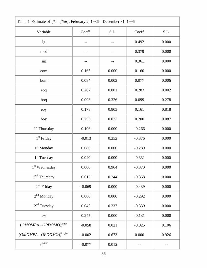
While the data in Table 1 suggest that the Desk follows the operating procedure

relatively closely, it did not follow the procedure mechanically. The correlation between

and is 0.61.tOPDOMO tOMOMPA 11 Figure 1 presents a scatter plot of these variables

11 Because the operating procedure is directed at the quantity of reserves over the maintenance period, it is not surprising that the correlation between and is considerably lower, 0.46. tOPDOMO tOMOD

8

with on the horizontal axis and on the vertical axis. These data

indicate that the Desk generally added less than the procedure indicated when the

procedure indicated that reserves be added and drained less than the procedure suggested

when it suggested reserves be drained. This behavior is due in part to the fact that the

Desk often does nothing when the procedure suggests a relatively small need to add or

drain reserves.

tOPDOMO tOMOMPA

It is also due, in part, to the fact that the Desk underestimated reserve demand on

average. The average forecast error is $0.07 billion, with a standard deviation of $0.37

billion. The forecast errors are slightly skewed upward, as the median is $0.06 billion,

and are highly serially correlated (0.83).12 While the mean and median forecast errors

are both significantly different from zero at the 5 percent significance level, they are

small relative to the mean ($54.6 billion) and median ($56.8 billion) levels of total

reserves. Hence, the Desk did a good job of forecasting reserve demand.

2.2 How Well Did the Desk Follow Its Operating Procedure?

The extent to which the Desk followed its operating procedure and the extent to

which the Desk responded to other factors in conducting daily open market operations are

formally investigated by estimating the equation

(5) t tOMOMPA OPDOMO zt tα β ε− = + + ,

where denotes a vector of factors that might cause the Desk to deviate from its

operating procedure and

tz

tε denotes the effect of all factors not reflected in . If the

Desk followed the operating procedure perfectly, then

tz

0tα β ε= = = .

12 Daily total reserves are available only for the period January 2, 1986-December 31, 1996. These statistics are based on the official measures of required and excess reserves for the period.

9

2.2.1 Factors that may have caused the Desk to respond differently

There are a number of factors that might cause the Desk to deviate from its

operating procedure. For example, demand for reserves is determined by banks’ reserve

requirements over a two-week period ending on the Monday, two days before settlement

Wednesday. Hence, on the last two days of the maintenance period, the demand for

reserves is perfectly interest inelastic. Because the demand for reserves is fixed on these

days, the Desk might behave somewhat differently on these days. The Desk may also

behave differently on various days of the year, such as the first and last days of the

month, quarter, or year, or the day of the maintenance period. Indeed, Hamilton (1997),

Thornton (2001a), Carpenter and Demiralp (2005), and Demiralp and Farley (2005)

report statistically significant day-of-the-maintenance-period and day-of-the-year effects

for various aspects of open market operations. These possibilities are investigated by

including dummy variables for each day of the maintenance period and for the first and

last days of the month, quarter, or year, and by partitioning by the day of the

maintenance period.

tOPDOMO

Table 1 suggests that the Desk may follow the operating procedure more closely

when it indicates that reserves should be added than when it indicates that reserves should

be drained. To investigate this formally, the day-of-the-maintenance-period dummy

variables are partitioned according to whether is positive or negative. tOPDOMO

Because of the difficulty in estimating reserve demand, the Desk might look to the

recent behavior of the funds rate or other signals of current market conditions in

conducting daily open market operations. The Desk takes a reading on the funds rate just

prior to the morning call. The morning call is a telephone conference among the staffs of

10

the Board of Governors, the Desk, and one of Federal Reserve Bank presidents. All

parties have access to the reserve projections, and the Desk outlines its intentions for that

day’s open market operation. One element of the call is where the funds rate is trading

“at the time of the call.” There are no transcripts of these calls; however, Thornton

(2006) documents that the rate at the time of the call was used as a check on the Desk’s

estimates of reserve demand. Hence, it is reasonable to conjecture that the Desk might

respond differently depending on the difference between the funds rate at the time of the

call and the funds rate target, call fftar− .

It seems likely that the Desk does not follow its procedure on days when the funds

rate target is adjusted. Conceptually, the Desk’s operating procedure is conditional on

the funds rate target. Consequently, a change in the target should have an effect on the

estimate of the quantity of reserves demanded; however, it may be difficult to estimate

the effect of a target change on the quantity of reserves demanded. Moreover, because

the demand for reserves is fixed on the last two days of the maintenance period, exactly

how the Desk would behave relative to the operating procedure on those days is

uncertain.

Finally, Hamilton (1997) has argued that the Fed responds to forecast misses in

one of the components of tν —the Treasury’s balance with the Fed. Specifically,

Hamilton suggests that if the Treasury’s balance were $400 million lower than expected,

the Desk would add x for each of the n remaining days in the maintenance period to make

up for that day’s error in forecasting the Treasury’s balance. If the forecast errors are

serially correlated, this information could be used in making today’s estimate of . To

my knowledge the forecast errors were never saved and analyzed. Consequently, it

tF

11

seems unlikely that the Desk engaged in the explicit error-correction behavior that

Hamilton describes. In any event, if it did, it should have also responded to the previous

day’s difference between actual bank borrowing and the IBA because borrowing is

highly serially correlated and the IBA was changed relatively infrequently.

2.2.2 Empirical Results

Equation 5 was estimated accounting for the factors noted above. Estimates of tν

are those used by Carpenter and Demiralp (2005) and were provided by the authors.

These data are available only beginning in January 1986; consequently, the estimation

period is January 2, 1986, through December 31, 1996. There is only an estimate of the

net forecast error for all components. There is a separate estimate for the Treasury’s

balance at the Fed. Hence, the Board of Governors’ forecast error for Treasury balances

on the previous day ( ) is also included. With this addition, the coefficient on 1( )tFE Tbal −

1tν − should reflect the explicit error correction behavior of the Desk for the remaining

factors, while the coefficient on 1( )tFE Tbal − reflects the explicit error-correction

behavior with respect to Treasury balance forecast errors.

Finally, at its first meeting in 1994, the FOMC began announcing policy actions

upon taking them. Because of this, and because banks began implementing deposit sweep

programs that reduced the demand for reserves about the same time, estimates of (5) are

presented for periods both before and after 1994. Also, the announcement came later in

the day after the Desk had conducted that day’s open market operations. Consequently,

for analyses of the effect of changes in the funds rate target on Desk operations, the

change in the funds rate target are aligned to the first day that the Desk could have

responded to the FOMC’s action.

12

The estimates are presented in Table 2. The equation was estimated using a

Newey-West estimator of the covariance matrix. The coefficient estimates are reported

in one column and the significance level associated with the null hypothesis that the

coefficient is zero is reported in the adjacent column. While a formal test of the null

hypothesis of temporal stability is easily rejected, the results for the two periods are

remarkably similar. Consistent with Table 1, during both periods the Desk adds less than

the procedure indicates when the procedure indicates that reserves should be added and

drains less when the procedure indicates reserves be drained. Moreover, during both

periods, the absolute value of the coefficients on the day-of-the-maintenance-period

dummy variables decline nearly monotonically from the first to the last day of the

maintenance period. Moreover, the Desk does not systematically deviate from its

operating procedure at the beginning or end of the quarter, or year, during either period.

The Desk’s response on the on the first and last days of the month are similar during both

periods; however, the response at the end of the month is clearly not statistically

significant for the post-1994 period.

There are some differences in the Desk’s response to other information.

Specifically, during the pre-1994 period the Desk deviated from the operating procedure

on days when the funds rate was changed—except on the last two days of the

maintenance period when reserve demand was fixed. In contrast, after 1994, there is no

statistically significant deviation from the operating procedure when the funds rate target

is changed. This finding is consistent with Taylor (2001) and Thornton (2001a). There

13

was no attempt to alter the supply of reserves immediately after the FOMC began the

practice of announcing policy actions.13

The estimates also suggest that the Desk relied more on the behavior of the funds

rate at the time of the call after 1994 than it did before 1994. The point estimate indicates

that on average the Desk added about $0.5 billion more than the operating procedure

suggested for every percentage point deviation of the funds rate from the target at the

time of the call. While the estimate is small given the size of the daily market for federal

funds, it nevertheless indicates that the Desk behaved in a manner consistent with

keeping the funds rate close to the target after 1994.

Finally, there is no evidence of explicit error correction by the Desk during either

period. The coefficient on 1tν − is negative but not statistically significant at the 5 percent

level for either period. The coefficient on 1( )tFE Tbal − is negative for the pre-1994

period, but again not statistically significant. Likewise, the coefficients on 1 1t tBR IBA− −−

are negative but not significantly different from zero in either period.

3. The Liquidity Effect

The liquidity effect—the decline in nominal interest rates associated with an

exogenous, central-bank-engineered increase in the monetary base—has received

relatively little empirical support historically (e.g., Pagan and Robertson, 1995; and

Thornton, 1988, 2001ab, 2006). The Desk’s open market data provide a unique

opportunity to investigate the extent to which Fed actions influence the federal funds rate.

If the Fed acts to change the equilibrium funds rate through open market operations, there

13 I do not say “announcing changes in the funds rate target” because the FOMC had not formally acknowledged that it was targeting the funds rate at this time. See Thornton (2005) for details.

14

should be a marked change in open market operations on days when the funds rate target

is changed.

The estimates reported in Table 2 suggest that the Desk behaved in a manner

consistent with the liquidity effect prior to 1994, but not after. Specifically, the Desk

added about $0.3 billion fewer reserves than the procedure suggested when the funds rate

target was increased by 25 basis points before 1994.14 This estimate suggests that the

demand for federal funds is very interest inelastic—a very small exogenous change in

reserves generates a relatively large change in the funds rate. If the demand for reserves

is this inelastic, however, one has to wonder why the liquidity effect has been so elusive.

Hence, the remainder of this section investigates the liquidity effect in a variety of ways.

3.1 Changes in Estimates of Reserve Demand

Consistent with the conventional view, the results in Table 2 suggest that, before

1994 but not after, the Desk drained more reserves than the operating procedure

suggested when the funds rate target was increased and added more when the target was

reduced. The size of the estimated coefficient for the pre-1994 period is relatively small,

however. A potential explanation for the small coefficient is that, because the Desk’s

estimates of reserve demand are conditional on the funds rate target, the Desk reduces its

estimate of the quantity of reserves demanded on days when the target is increased and

increases its estimate on days when the target is reduced. There were 88 changes in the

funds rate target during the sample period (43 increases and 45 decreases). Of these, 78 14 Demiralp and Jorda (2002) investigate the liquidity effect using a similar methodology. Specifically, they estimate the response of open market transactions of various types to surprise changes in the funds rate target for a sub-period of the period April 25, 1984 through August 14, 2000. They find evidence that they interpret as being “broadly consistent with the traditional liquidity effect” prior to 1994 but not after. Recently, however, de Jong and Herrera (2004) have re-evaluated Demiralp and Jorda’s work. Consistent with the findings presented here, they find no evidence consistent with a liquidity effect over the entire sample period, but find evidence consistent with a liquidity effect for a sub-period after August 18, 1998, when lagged reserve accounting was reintroduced.

15

occurred prior to 1994 and 10 after. Figures 2 and 3 present the revisions to reserve

demand when the funds rate target was increased or decreased, respectively. These data

are not consistent with the idea that the Desk revises its estimate of reserve demand

systematically in response to a change in the target. Figure 2 shows that there were only

six occasions when reserve demand was revised down by $0.5 billion or more when the

target was increased, while there were four days when it was revised up by a

corresponding amount. Likewise, Figure 3 shows that estimates of reserve demand were

not systematically revised up in response to a decrease in the target. Indeed, most often

the estimates were essentially unrevised, despite the change in the target. Hence, the

relatively small estimated coefficient in Table 2 is not the consequence of systematic

revisions of reserve demand.

3.2 The Desk’s Behavior when the Funds Rate Target Is Changed

The results in the previous section indicate that the Desk deviated significantly

from its operating procedure when the target was changed, at least prior to 1994. This

result is investigated more fully in Figures 4 and 5, which show scatter plots of

vs. on days when the funds rate target was decreased and

increased, respectively. If the Desk causes the funds rate to fall, there should be many

more observations above the 45-degree line than below in Figure 4. This is not the case,

however. Likewise, if the Desk causes the funds rate to rise, there should be many more

observations below the 45-degree line than above in Figure 5. While this is the case, as

we have already noted, the procedure was skewed toward adding rather than draining

reserves. Moreover, Figure 1 shows that the Desk generally added significantly less than

the procedure suggested on all days when the procedure indicated reserves should be

OPDOMO OMOMPA

16

added. Consequently, it is not clear whether Figure 5 represent a significant change in

the Desk’s behavior on days when the target was increased.

To investigate whether the Desk behaved significantly differently when the funds

rate target was changed, 10,000 samples (sizes 43 and 45) were obtained by

bootstrapping the 3088 observations of OMOMPA OPDOMO− on days when the target

was not changed. Table 3 reports the 90 percent coverage intervals for the mean, median,

and standard deviation of these samples along with the same sample statistics for days

when the funds rate target was changed. The results suggest that the Desk did not change

its behavior significantly when the funds rate target was increased. Five of the six sample

statistics are well within the corresponding 90 percent coverage intervals. The sample

mean of the 45 days when the target was decreased lies outside of the 90 percent

coverage interval, suggesting that the Desk added significantly more reserves on average

than the operating procedure indicated when the target was decreased. Because the

distributions of are skewed, the median is a better measure of

central tendency. The sample statistic for the median is well within the coverage interval,

suggesting that the Desk did not behave differently when the target was decreased.

Hence, there is weak evidence that suggests the Desk attempted to engineer decreases in

the funds rate.

OMOMPA OPDOMO−

3.3 Implementing a Target Change over Time

It might be the case that the Desk does not take all the operations necessary to

change the funds rate on the day the target is changed. Instead, the Desk may add or

drain reserves over several days to bring about the change in reserves necessary to sustain

the funds rate at the new target level (e.g., Taylor, 2001).

17

This possibility is investigated by comparing the five-day averages of

for five days before each target change and for the day of the

target change and four days after the change. The five-day averages are plotted in

Figures 6 and 7 for increases and decreases in the funds rate target, respectively.

OMOMPA OPDOMO−

15 If the

Desk pursued the increase in the funds rate, there should be more observations below the

45-degree line than above in Figure 6. Similarly, if the Desk pursued the decrease in the

funds rate, there should be more observations above the 45-degree line than below in

Figure 7. This is not the case. In both instances, the number of observations above and

below the 45-degree line is nearly equal. Moreover, simple tests of the equality of the

means, medians, and variances of the distributions before and after target changes cannot

reject the null hypothesis of equality at even the 10 percent significance level for either

positive or negative target changes. Consequently, there is no evidence that the Desk

implemented target changes over a period of five days. It is important to note that the

conclusion is the same for both increases and decreases in the target. Hence, if the Desk

engineered increases in the funds rate target, it completed the operations necessary to

effect these changes quickly.

3.4 Estimating the Liquidity Effect Directly

The conventional way to estimate the liquidity effect is to regress changes in the

interest rate on a variable that represents an exogenous change in reserves or monetary

policy. Hamilton (1997) used this approach and found evidence of a statistically

significant liquidity effect of exogenous changes in reserves on the federal funds rate.

His measure of a supply shock was his estimate of the forecast error the Desk makes in

15 There were 14 occasions (eight for positive and six for negative changes in the target) when there were fewer than 5 days between successive target changes. These changes were deleted so as not to bias the results.

18

forecasting the Treasury’s balance with the Fed. Hamilton found the liquidity effect to be

statistically significant, but only on settlement Wednesdays. Thornton (2001a) notes

three problems with this analysis. First, the slope of the reserve demand function (and,

therefore, the liquidity effect) cannot be estimated on settlement Wednesdays because of

the two-day lag in the Fed’s reserve accounting system. Second, what matters on the last

day of the maintenance period is the imbalance of reserve supply and demand on average

over the maintenance period. Because a 1-day error in forecasting the Treasury’s balance

contributes only one-fourteenth of the average error, it would take a very large shock to

the Treasury’s balance on the last day of the maintenance period to generate a large

maintenance-period-average reserve imbalance. Finally, Thornton notes that Hamilton

used an estimate of the Desk’s forecast error, not the actual forecast error.16 Thornton

(2001a) goes on to show that Hamilton’s settlement-Wednesday liquidity effect was

idiosyncratic to his sample period and, even during Hamilton’s sample period, it is

attributable to just six observations when the funds rate changed by a large amount on

settlement Wednesdays.

Carpenter and Demiralp (2005) attempt to overcome some of the data

shortcomings of Hamilton’s analysis by using a more comprehensive measure of a

reserve supply shock. Specifically, they use an estimate of tν based on the Board of

Governors’ estimate of .tF 17 They find a statistically significant liquidity effect on six of

the ten days during the maintenance period over the period May 18, 1989-January 30,

2004. As with Hamilton’s findings, the estimated liquidity effect is largest on settlement 16 See Thornton (2004b) for analysis of the Desk’s forecast error and comparison of those errors with Hamilton’s estimates. 17 They kindly provided me with these forecast errors, which cover the period January 2, 1986, to June 30, 2000, for the Board of Governors’ estimates and December 23, 1993, through June 30, 2000, for the New York Fed’s estimates.

19

Wednesday when, contrary to Carpenter and Demiralp’s assertion, the slope of the

demand for reserves cannot be estimated.18

The effects of shocks to reserves on the funds rate is investigated here using

Carpenter and Demiralp’s data. Figure 8 presents a scatter plot of the ( )tff fftar− and

the Board of Governors’ estimate of over the period January 2, 1986, through

December 31, 1996. Days when

tv

tν was not available and the last two days of 1986,

when ( )tff fftar− was more than 8 percentage points, are deleted, leaving 2676 daily

observations. While not obvious from Figure 8, there is a weak negative relationship

between tν and ( )tff fftar− . The correlation is -0.124. Carpenter and Demiralp (2005)

suggest that the relationship between supply shocks and the funds rate is non-linear,

finding that their statistically significant liquidity effect is due to large supply shocks (≥

$1 billion). Hence, the relatively low correlation could be due to the fact that most often

supply shocks are relatively small. There is some evidence of this. When only days for

which the absolute value of the supply shock is greater than $2 billion (180 observations)

are considered, the correlation doubles to -0.215. Nevertheless, even for large reserve

supply shocks the relationship between reserve supply shocks and the funds rate appears

weak.

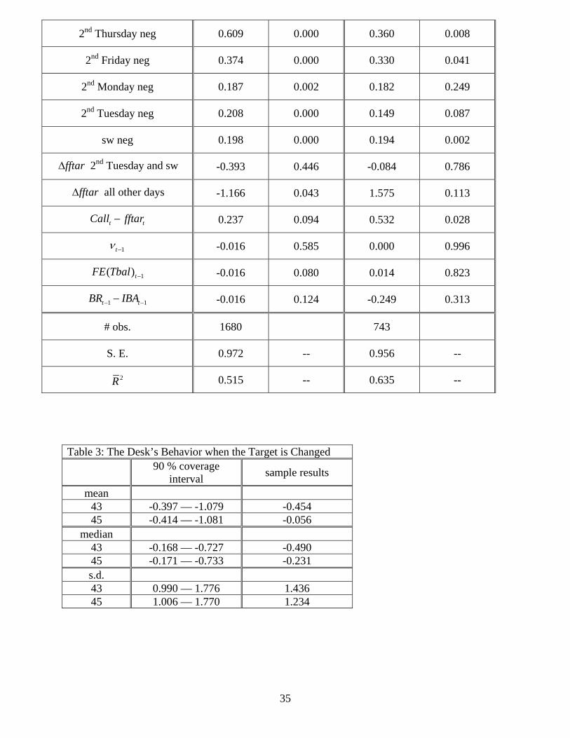
To investigate this possibility further, Table 4 presents the results for a regression

of ( )tff fftar− on day-of-the-year and day-of-the-maintenance-period dummy variables,

, and ( tOMOMPA OPDOMO− ) tν , over the period January 2, 1986 – December 31,

1996. Like shocks to reserve supply, one might expect that if the Desk adds more

18 The slope of the demand curve cannot be estimated during any of the days of the maintenance period after August 1998, when the Fed returned to lagged reserve accounting.

20

reserves than the operating procedure indicates, the funds rate might fall, and vice versa.

Given the previous results, ( )tOMOMPA OPDOMO− and tν are partitioned into days

when the funds rate target was and was not changed. Consistent with Carpenter and

Demiralp’s finding, there is a negative and statistically significant relationship between

( t)ff fftar− and tν . Surprisingly, the absolute value of the estimate is nearly twice as

large on days when the funds rate target was changed than when it was not.19

The results also suggest that the funds rate will decline if the Desk adds or drains

more reserves than the operating procedure indicates is necessary. The coefficients are

not statistically significant, however.

Following up on Carpenter and Demiralp’s finding of non-linearity in the effect of

supply shocks on the funds rate, tν is partitioned into days when the corresponding

shocks are large ( l , ≥ $2 billion), medium ( , > $1 billion but < $2 billion), and small

( , ≤ $1 billion). In order to guarantee that the effect is due to non-linearity and not to

an intercept shift, dummy variables are included for each of these partitions. The

estimates, also presented in Table 4, confirm Carpenter and Demiralp’s finding.

m

s

20

Specifically, while the effect of tν on the funds rate is nearly always negative, it is

statistically significant only for large supply shocks. Moreover, it is only on days when

the target is not changed. The coefficient is larger for days when the target was changed,

but not statistically significant at the 5 percent level. It is important to note that it takes a

relatively large supply shock to have a statistically significant impact on the funds rate.

19 The results are very similar if the sample ends on December 31, 1993; hence, the results for the shorter sample are not presented here. 20 The equation was also estimated allowing for corresponding shifts in the intercept. The qualitative results were unchanged, so only the results that do not include corresponding shifts in the intercept are presented here.

21

Consequently, in contrast with the implications of the estimates from Table 2, these

estimates suggest that the demand for reserves is relatively interest elastic. As noted

above, shocks this large are relatively rare events. However, it is worth noting, that when

tν is partitioned by size, with the exception of settlement Wednesday, day-of-the-

maintenance-period differences in the behavior of the funds rate are significantly reduced

and become statistically significant. Hence, there appears to be some relationship

between large supply shocks and days of the maintenance period.

There are two reasons these findings do not support Carpenter and Demiralp’s

assertion that the response of the funds rate to supply shocks provides “strong evidence of

a liquidity effect at the daily frequency.” First, consistent with Figure 8, reserve supply

shocks account for very little of the daily variability of the funds rate from the target.

Indeed, if tν is omitted from the equation, 2R declines by less than one one-hundredth of

a percentage point. Second, and most important, while the estimates suggest that large

shocks to reserves are associated with changes in the equilibrium funds rate, such

estimates provide no evidence for the more interesting and policy-relevant question of

whether the Fed brings about permanent changes in the funds rate through open market

operations. Indeed, the estimates suggest that it is unlikely that the Fed does this. There

were only 554 days in the entire sample of 3176 daily observations when the Desk

deviated from its operating procedure by $2.0 billion or more. Moreover, the estimates

suggest that the largest deviation (-$9.19 billion) would have generated about a 42-basis-

point rise in the funds rate. Hence, these estimates suggest that it would take a series of

relatively large open market operations in one direction to bring about the kind of

changes in the equilibrium funds rate that the Fed is often credited with engineering. As

22

we have already noted, there is no evidence that the Desk engaged in such open market

operations upon changing the funds rate target.

3.5 The Liquidity Effect and the Federal Funds Market

As a general rule, the larger a single market participant’s activities are in the

market, the larger should be the effect of such activities on equilibrium price. Indeed, the

hypothesis of atomistic market participants is a cornerstone of the competitive market

model. As a general rule, one would expect the Fed’s ability to influence the federal

funds rate to be positively related to the relative importance of its activities in the federal

funds market—the more liquidity the Fed provides to the market, the larger should be its

ability to affect the equilibrium federal funds rate. Hence, some additional evidence on

the potential for a liquidity effect can be obtained by investigating the relative importance

of open market operations in the federal funds market.

Despite the importance of the federal funds rate in the conduct of monetary

policy, surprisingly little is known about it. Federal funds transactions involve the

purchase or sale of deposit balances at the Fed. Hence, direct market participation is

limited to entities that hold deposits at the Fed. For the federal funds market, this means

banks, Fannie Mae, Freddie Mac, and Federal Home Loan Bank.21 There are both

brokered and non-brokered transactions in the market.22 Until recently relatively little

was known about the overall size of the market. Using estimated data from Fedwire

funds transfers during the first quarter of 1998, Furfine (1999) estimates the average daily

volume of federal funds transactions to be $144 billion. Recently, Demiralp, Preslopsky,

21 Fannie Mae, Freddie Mac, and Federal Home Loan Bank were major players in the federal funds market and often had zero or near zero balances with the Fed at the end of the day. 22 See Stigum (1990), Furfine (1999), and Demiralp, Preslopsky, and Whitesell (2004) for discussions of various aspects of the federal funds market.

23

and Whitesell (2004) have used a modification of Furfine’s methodology to estimate the

size of the funds market over the period 1998 – 2003. They find that the average daily

volume of transactions in the funds market in the first quarter of 1998 was $145 billion,

and that the daily volume of federal funds transactions increased until 2001 and then

declined slightly.

Knowledge of the division of the market between brokered and non-brokered

trading is less well known. Stigum (1990) suggested that the brokered funds market was

about $70 billion per day in the late 1980s; however, Furfine (1999) found that about 83

percent of the identified federal funds transactions were brokered.

The published federal funds rate is a quantity-weighted average of transactions of

a group of brokers that report their transactions daily to the Federal Reserve Bank of New

York. The 30-day moving average of the total volume of federal funds transactions

reported by these brokers for the period January 1, 1987, through December 31, 1993, is

presented in Figure 9. The trading volume hovered around $53 billion from the

beginning of 1987 to mid-1990 and then increased dramatically by about $10 billion.

Trading volume peaked in October 1990 and then began to decline. The initial decline in

trading volume coincides with the elimination of reserve requirements on non-personal

time and savings deposits, which reduced reserve demand by about $13.5 billion. The

sharp decline in 1992 also coincides reasonably well with the reduction in percentage

reserve requirements from 12 to 10 percent.23 Why trading volume trends down

beginning in 1991 is unclear, however.

23 It is also the case that the number of brokers has changed over time. Unfortunately, there is no precise dating of changes in the number of participating brokers.

24

In any event, these volume figures suggest that the brokers who report daily to the

Federal Reserve Bank of New York account for a relatively small share of the brokered

market, and an even smaller share of the total market. Indeed, based on Furfine’s and

Demiralp, Preslopsky, and Whitesell’s estimates, the brokers that report daily to the Fed

account for roughly about a third of the federal funds market.

Despite the possibility that the brokered transactions appear to represent a

relatively small share of the federal funds market, these are the correct data for analyzing

the relative importance of open market operations because these data are used to calculate

the effective federal funds rate—the rate used in virtually all analyses of monetary policy.

The day-to-day variation in the volume of trading among these brokers is

relatively large. There are only four days in this sample when the daily change in the

trading volume is $5 billion or less. In contrast, there were only 267 of the 3176 days

where the absolute value of was larger than $5.0 billion. It is hardly surprising,

therefore, that OMOD accounts for almost none of the daily variation in the volume of

federal funds transactions.

OMOD

The relatively small size of open market operations alone may account for the

results presented above. But there are other reasons for suspecting that the impact of

open market operations on the funds rate is small. While seldom discussed in analyses of

open market operations and the federal funds rate, in reality the link between open market

operations and the funds rate is second-order. Open market operations do not directly

affect the supply of federal funds. Rather, they directly affect the supply of reserves

available to banks. Banks need not automatically increase or decrease federal funds

trading when open market operations alter the availability of reserves. Nevertheless,

25

because the initial effect of open market operations is on the reserves of large banks,

some of whom may act as brokers in the federal funds market, simultaneously buying and

selling funds (e.g., Furfine, 1999), it is reasonable to assume that open market operations

will likely impact the availability of funds in the market.

Nevertheless, it is important to remember that the volume of federal funds trading

is determined by a variety of factors that are independent of daily open market

operations. For example, Meulendyke (1998) notes that beginning in the 1960s, when

short-term rates rose above Regulation Q interest rate ceilings, large banks began

financing their longer-term lending in the overnight market. It is now recognized that

many banks finance a significant part of their loan portfolio in the overnight markets. It

is also well known that large banks tend to be net demanders of funds, while small banks

tend to be net suppliers. Hence, daily changes in the volume of federal funds transactions

are likely to be affected by changes in the distribution of deposit and reserve flows

unrelated to daily open market operations.

Not only is the daily volume of federal funds transactions large relative to daily

open market operations, it is many times larger than the overnight reserve balance at the

Fed—the commodity being traded (e.g., Taylor, 2001). While the exact source of the

disparity between the flow of federal funds transactions and the stock of the commodity

being traded is unclear, there can be little doubt that the flow of federal funds transactions

is only weakly linked to the stock of the commodity being traded.24

24 The large flow of federal funds relative to the daily volume of balances at the Federal Reserve would appear to be inconsistent with Demiralp and Farley’s (2005, p. 1132) characterization of open market operations and the equilibrium federal funds rate. They suggest that open market operations “are used to bring the supply of balances at the Federal Reserve in line with the demand for them at an interest rate (the federal funds rate) near the level specified by the Federal Open Market Committee (FOMC).”

26

Finally, since the early 1980s the Desk has followed the practice of entering the

market once per day—before January 1987 this occurred about 11:30 EST. Federal funds

transactions occur continuously throughout the day. Indeed, spikes in the funds rate that

are often associated with settlement Wednesdays are thought to be due to trading that

occurs later in the day. In any event, if open market operations were to have a significant

effect on the funds rate, one might expect the effect to occur around the time that the

Desk is in the market. Hence, the extent to which these activities would affect the

transactions-weighted-average of transactions rates over the day is difficult to say.

While the effect of open market operations on the funds market and,

consequently, the funds rate, is indirect and uncertain, their effect on total reserves is not.

Moreover, conceptually, open market operations affect the funds rate by causing banks to

buy or sell funds when the supply of reserves is decreased or increased, respectively,

through open market operations. Hence, the relative importance of open market

operations can be gauged by seeing how much of the variation in daily changes in total

reserves they account for. To this end, changes in total reserves are regressed on changes

in the Desk’s estimate of reserve demand and reserve supply, changes in borrowing,

errors in forecasting autonomous factors that affect reserves, and daily open market

operations. The results, reported in Table 5, show that changes in total reserves are

positively and significantly related to daily open market operations. Indeed, when

is deleted from the equation, tOMOD 2R decreases from 0.2602 to 0.1736, suggesting

that accounts for nearly 10 percent of the daily changes in total reserves. This

simple analysis suggests that, while important, ’s contribution to changes in total

tOMOD

tOMOD

27

reserves is quantitatively small. Given their relatively small effect on total reserves, it is

not surprising that open market operations have an even smaller effect on federal funds.

4.0 Analysis and Conclusions

Our analysis of the Desk’s use of its operating procedure over the period March 1,

1984, through December 31, 1996, indicates that the Desk relied on the operating

procedure in conducting daily open market operations. Indeed, the operating procedure

alone accounts for nearly 40 percent of open market operations conducted during this

period. The operating procedure and other factors—such as day-of-the-maintenance-

period and day-of-the-year effects, differences between the funds rate and the funds rate

target just prior to open market operations, and changes in the funds rate target—account

for more than 50 percent of the variation in daily open market operations. Although

large, these estimates indicate that there are other important factors that cause the Desk to

deviate from its operating procedure.

Contrary to conventional wisdom—that the Fed controls the federal funds rate

through open market operations—we have found little support of an important liquidity

effect at the daily frequency. While there is some evidence of a statistically significant

negative relationship between reserve supply shocks and the funds rate, the relationship is

weak. Consequently, to move the funds rate by 25 basis points or more, it appears that

the Desk would have conduct considerably larger open market operations than it has in

fact conducted.

One possible reason for this finding is that changes in the funds rate target were

anticipated. However, after conducting an extensive analysis of press reports, Poole,

Rasche, and Thornton (2002, p. 73) found “little indication that the market was aware

28

that the Fed was setting an explicit objective for the federal funds rate before 1989.” This

is not surprising in that Thornton (2006) shows that the FOMC was reluctant to

acknowledge that it was targeting the funds rate. Moreover, Poole, Rasche, and Thornton

(2002) show that the market frequently did not know that policy had changed when the

Fed changed the target during 1989 and 1990 and that the target changes prior to 1994

were generally not predicted. Furthermore, prior to 1994, most funds rate target changes

occurred during the intermeeting period (the period between consecutive FOMC

meetings) and, hence, would have been difficult to predict exactly even if the market

knew the Fed was targeting the funds rate and was expecting a target change.

Consequently, it is extremely unlikely that rational expectations accounts for the lack of

evidence of a liquidity effect.

Another possible explanation for the lack of evidence of a liquidity effect is that

target changes are implemented over a period of several days, not immediately (e.g.,

Taylor, 2001). The analysis presented here finds no support for this explanation,

however.

Yet another explanation for this finding is that open market operations account for

a very small proportion of the variation in the equilibrium quantities in the reserves and

federal funds markets. This explanation is supported by the fact that open market

operations explain relatively little of the maintenance-period variation in total reserves

and an extremely small amount of the daily variation in daily volume of federal funds

transactions.

One explanation not investigated here is that some, and perhaps many, changes in

the funds rate target are endogenous. Economic theory suggests that the Fed cannot

29

control the natural rate of interest. Hence, when market forces bring about changes in

inflation expectations or the real rate, the Fed can either change its target or permit policy

to become inadvertently tighter or easier, depending on whether market forces are driving

interest rates down or up. In any event, if target changes represent a response of the Fed

to changing conditions that affect nominal interest rates rather than an exogenous change

engineered to achieve some policy objective, the Desk would not necessarily have an

incentive to add or drain reserves aggressively when the target is changed. Elsewhere

(Thornton, 2004b), I have presented evidence that many of the target changes identified

in an influential paper by Cook and Hahn (1989) were endogenous. A proper

investigation of this possibility during this period is left for future research.

Finally, I would note that evidence that the liquidity effect is small and

statistically unimportant does not mean that the Fed could not move interest rates if it

desired. It merely suggests that the Fed has not done so. Given their direct effect on

reserves and the corresponding effect of changes in reserves on banks, one can

understand why the Fed might be reluctant to engage in large open market operations.

This reluctance would be particularly strong if the Fed is a small enough player in the

credit market that it would take very large open market operations to generate significant

changes in the equilibrium short-term rates.

30

References:

Carpenter, S. and Demiralp, S. (2005). “The Liquidity Effect in the Federal Funds Market: Evidence from Daily Open Market Operations,” Journal of Money, Credit, and Banking (2006).

Cook, T. and Hahn, T. (1989). “The Effect of Changes in the Federal Funds Rate Target

on Market Interest Rates in the 1970s,” Journal of Monetary Economics, November, 24(3), pp. 331-51.

de Jong, R., and Herrera, A. M. (2004). “Dynamic Censored Regression and the Open

Market Desk Reaction Function,” unpublished working paper. Demiralp, S., and Farley, D. (2005). “Declining Required Reserves, Funds Rate

Volatility, and Open Market Operations,” Journal of Banking and Finance, May, 29(5), pp. 1131-52.

Demiralp, S. Preslopsky, B. and Whitesell, W. (2004). “Overnight Interbank Loan

Markets,” Board of Governors of the Federal Reserve System working paper. Demiralp, S., and Jorda, O. (2002). “The Announcement Effect: Evidence from Open

Market Desk Data,” Economic Policy Review, May, 8(1), pp. 29-48. Sternlight, P. D. (1991). “Monetary Policy and Open Market Operations during 1990,”

Federal Reserve Bank of New York, Quarterly Review, Spring, 16(1), pp. 52-78. Sternlight, P. D. (1992). “Monetary Policy and Open Market Operations during 1991,”

Federal Reserve Bank of New York, Quarterly Review, Spring, 17(1), pp. 72-95. Friedman, B. M. (1999). “The Future of Monetary Policy: The Central Bank as an Army

with Only a Signal Corps?” International Finance, November, 2(3), pp. 321-38. Furfine, C. H. (1999). “The Microstructure of the Federal Funds Market,” Financial

Markets, Institutions & Instruments, December, 8(5), pp. 24-44. Hamilton, J. D. (1997). “Measuring the Liquidity Effect,” American Economic Review,

March 1997, 87(1), pp. 80-97. Meulendyke, A-M. (1998). U.S. Monetary Policy & Financial Markets, Federal Reserve

Bank of New York. Pagan, A. R., and Robertson, J. C. (1995). “Resolving the Liquidity Effect,” Federal

Reserve Bank of St. Louis Review, May/June, 77(3), pp. 33-54.

31

Poole, W., Rasche, R. H. and Thornton, D. L. (2002). “Market Anticipations of Monetary Policy Actions,” Federal Reserve Bank of St. Louis Review, July/August, 84(4), pp. 65-93.

Stigum, M. (1990). The Money Market, 3rd. ed. Homewood, Illinois: Dow Jones-Irwin. Taylor, J. B. (2001). “Expectations, Open Market Operations, and Changes in the Federal

Funds Rate, Federal Reserve Bank of St. Louis Review, July/August, 83(4), pp. 33-47.

Thornton, D. L. (2006). “When Did the FOMC Begin Targeting the Federal Funds Rate?

What the Verbatim Transcripts Tell Us,” Journal of Money, Credit, and Banking, 38(8), 2039-71.

Thornton, D. L. (2005). “A New Federal Funds Rate Target Series: September 27, 1982 –

December 31, 1993,” Federal Reserve Bank of St. Louis Working Paper 2005-032A.

Thornton, D. L. (2004b). “The Fed and Short-Term Rates: Is It Open Market Operations,

Open Mouth Operations or Interest Rate Smoothing?” Journal of Banking and Finance, March, 28(3), pp. 475-98.

Thornton, D. L. (2001a). “Identifying the Liquidity Effect at the Daily Frequency,”

Federal Reserve Bank of St. Louis Review, July/August, 83(4), pp. 59-78.

Thornton, D. L. (2001b). “The Federal Reserve’s Operating Procedure, Nonborrowed Reserves, Borrowed Reserves and the Liquidity Effect,” Journal of Banking and Finance, September, 25(9), pp. 1717-39.

Thornton, D. L. (1988). “The Effect of Monetary Policy on Short-Term Interest Rates,”

Federal Reserve Bank of St. Louis Review, May/June, 70(3), pp. 53-72.

32

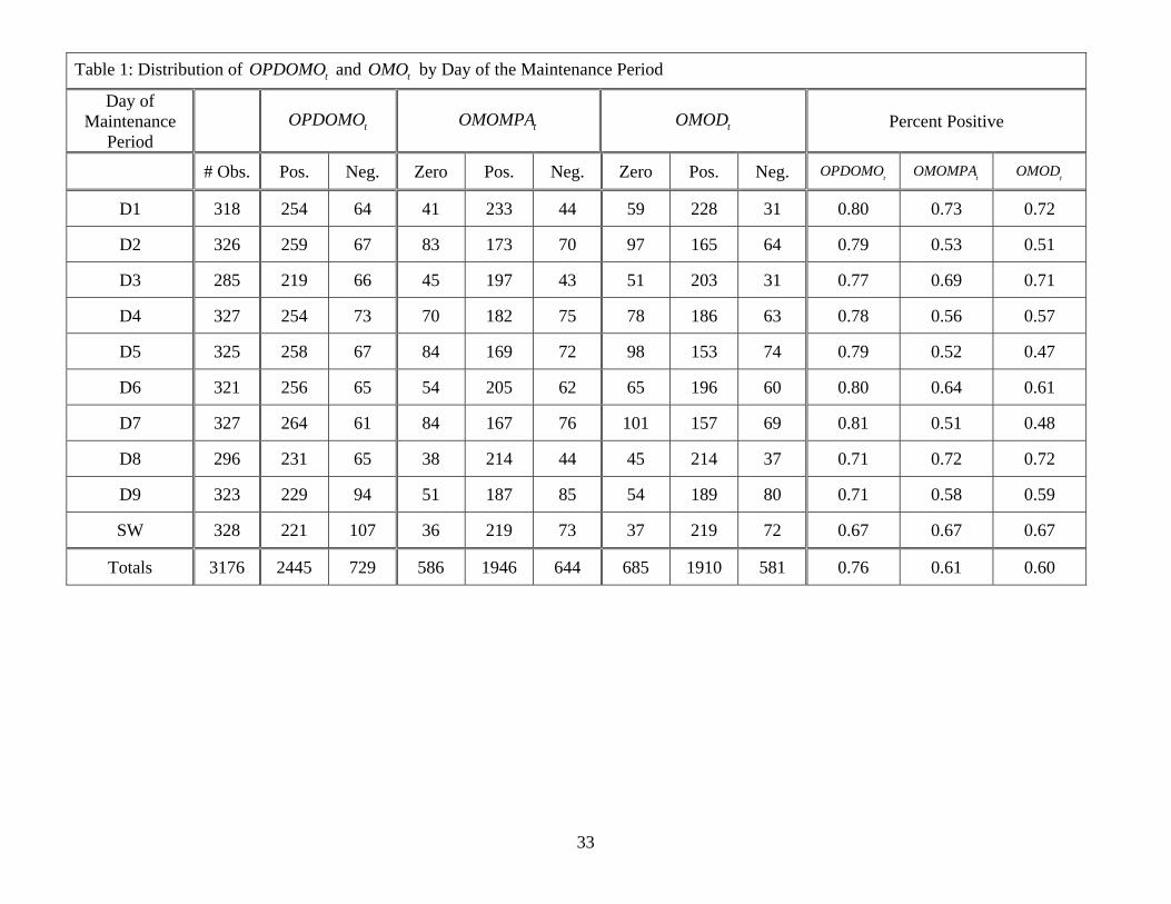
Table 1: Distribution of and by Day of the Maintenance Period tOPDOMO tOMO

Day of Maintenance

Period tOPDOMO tOMOMPA tOMOD Percent Positive

# Obs. Pos. Neg. Zero Pos. Neg. Zero Pos. Neg. tOPDOMO tOMOMPA tOMOD

D1 318 254 64 41 233 44 59 228 31 0.80 0.73 0.72

D2 326 259 67 83 173 70 97 165 64 0.79 0.53 0.51

D3 285 219 66 45 197 43 51 203 31 0.77 0.69 0.71

D4 327 254 73 70 182 75 78 186 63 0.78 0.56 0.57

D5 325 258 67 84 169 72 98 153 74 0.79 0.52 0.47

D6 321 256 65 54 205 62 65 196 60 0.80 0.64 0.61

D7 327 264 61 84 167 76 101 157 69 0.81 0.51 0.48

D8 296 231 65 38 214 44 45 214 37 0.71 0.72 0.72

D9 323 229 94 51 187 85 54 189 80 0.71 0.58 0.59

SW 328 221 107 36 219 73 37 219 72 0.67 0.67 0.67

Totals 3176 2445 729 586 1946 644 685 1910 581 0.76 0.61 0.60

33

Table 2: The Desk’s Use of the Operating Procedure: February 2, 1986 – December 31, 1996

Pre-1994 Post-1994

Variable Coeff. S.L. Coeff. S.L.

bom 0.272 0.014 0.313 0.051

eom 0.277 0.050 0.182 0.242

boq -0.198 0.365 -0.308 0.446

eoq -0.150 0.533 -0.504 0.188

boy -0.401 0.229 0.314 0.447

eoy -0.244 0.559 0.538 0.214

1st Thursday pos -2.135 0.000 -3.087 0.000

1st Friday pos -1.943 0.000 -2.905 0.000

1st Monday pos -1.590 0.000 -2.477 0.000

1st Tuesday pos -1.503 0.000 -2.212 0.000

1st Wednesday pos -1.434 0.000 -1.941 0.000

2nd Thursday pos -0.923 0.000 -1.188 0.000

2nd Friday pos -0.837 0.000 -0.943 0.000

2nd Monday pos -0.345 0.000 -0.365 0.000

2nd Tuesday pos -0.297 0.000 -0.329 0.000

sw pos -0.223 0.000 -0.148 0.002

1st Thursday neg 1.532 0.000 1.576 0.000

1st Friday neg 1.501 0.000 1.118 0.000

1st Monday neg 1.081 0.000 1.007 0.000

1st Tuesday neg 0.904 0.000 1.096 0.001

1st Wednesday neg 0.757 0.000 1.103 0.001

34

2nd Thursday neg 0.609 0.000 0.360 0.008

2nd Friday neg 0.374 0.000 0.330 0.041

2nd Monday neg 0.187 0.002 0.182 0.249

2nd Tuesday neg 0.208 0.000 0.149 0.087

sw neg 0.198 0.000 0.194 0.002

fftarΔ 2nd Tuesday and sw -0.393 0.446 -0.084 0.786

fftarΔ all other days -1.166 0.043 1.575 0.113

t tCall fftar− 0.237 0.094 0.532 0.028

1tν − -0.016 0.585 0.000 0.996

1( )tFE Tbal − -0.016 0.080 0.014 0.823

1 1t tBR IBA− −− -0.016 0.124 -0.249 0.313

# obs. 1680 743

S. E. 0.972 -- 0.956 --

2R 0.515 -- 0.635 --

Table 3: The Desk’s Behavior when the Target is Changed

90 % coverage interval sample results

mean 43 -0.397 — -1.079 -0.454 45 -0.414 — -1.081 -0.056

median 43 -0.168 — -0.727 -0.490 45 -0.171 — -0.733 -0.231 s.d. 43 0.990 — 1.776 1.436 45 1.006 — 1.770 1.234

35

36

tTable 4: Estimate of tff fftar− , February 2, 1986 – December 31, 1996

Variable Coeff. S.L. Coeff. S.L.

lg -- -- 0.492 0.000

med -- -- 0.379 0.000

sm -- -- 0.361 0.000

eom 0.165 0.000 0.160 0.000

bom 0.084 0.003 0.077 0.006

eoq 0.287 0.001 0.283 0.002

boq 0.093 0.326 0.099 0.278

eoy 0.178 0.803 0.161 0.818

boy 0.253 0.027 0.200 0.087

1st Thursday 0.106 0.000 -0.266 0.000

1st Friday -0.013 0.252 -0.376 0.000

1st Monday 0.080 0.000 -0.289 0.000

1st Tuesday 0.040 0.000 -0.331 0.000

1st Wednesday 0.000 0.964 -0.370 0.000

2nd Thursday 0.013 0.244 -0.358 0.000

2nd Friday -0.069 0.000 -0.439 0.000

2nd Monday 0.080 0.000 -0.292 0.000

2nd Tuesday 0.045 0.237 -0.330 0.000

sw 0.245 0.000 -0.131 0.000

( ) fftartOMOMPA OPDOMO Δ− -0.058 0.021 -0.025 0.106

( )No fftartOMOMPA OPDOMO Δ− -0.002 0.673 0.000 0.926

fftartνΔ -0.077 0.012 -- --

No fftartν

Δ -0.032 0.005 -- --

,l fftartνΔ -- -- -0.102 0.020

,l No fftartν

Δ -- -- -0.045 0.031 ,m fftar

tνΔ -- -- -0.083 0.055

,m No fftartν

Δ -- -- -0.010 0.255 ,s fftar

tνΔ -- -- 0.008 0.847

,s No fftartν

Δ -- -- -0.034 0.076

# obs. 2678 -- 2678 --

S. E. 0.344 -- 0.342 --

2R 0.102 -- 0.111 --

Table 5: The Daily Change in Total Reserves: January 2, 1986 – December 31, 1996

Variable Coeff. S.L.

Const. -0.461 0.000

*1 ( ,t tE f ff x−Δ )t 0.688 0.000

1t tE NBR−Δ 0.558 0.000

tν 0.672 0.000

tBRΔ 0.846 0.000

tOMOD 0.373 0.000

# obs. 2677 --

S. E. 2.7542 --

2R 0.2602 --

37

Figure 1: Comparison of OPDOMO and OMOMPA March 1, 1984 - December 31, 1996

-4

-2

0

2

4

6

8

10

-6 -4 -2 0 2 4 6 8 10 12 14

OPDOMO (billions of $)

OM

OM

PA (b

illio

ns o

f $)

38

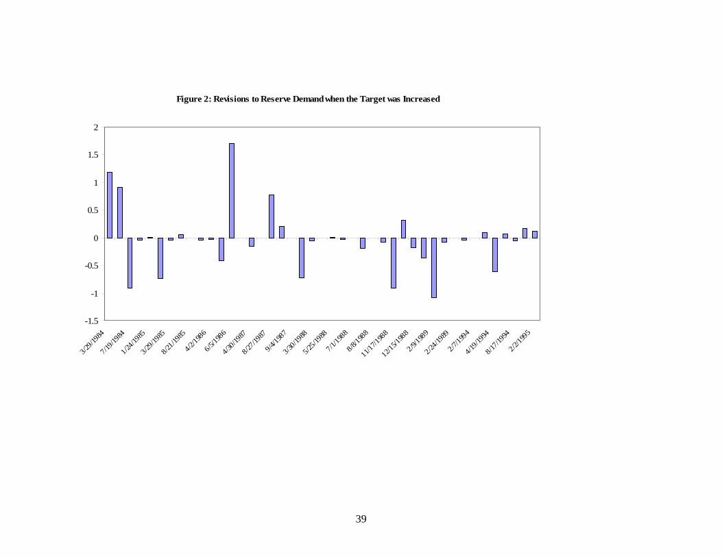
Figure 2: Revisions to Reserve Demand when the Target was Increased

-1.5

-1

-0.5

0

0.5

1

1.5

2

3/29/1

984

7/19/1

984

1/24/1

985

3/29/1

985

8/21/1

985

4/2/19

866/5

/1986

4/30/1

987

8/27/1

987

9/4/19

873/3

0/198

85/2

5/198

87/1

/1988

8/8/19

8811

/17/19

8812

/15/19

882/9

/1989

2/24/1

989

2/7/19

944/1

9/199

48/1

7/199

42/2

/1995

39

Figure 3: Revisions to Reserve Demand when the Target was Decreased

-2

-1.5

-1

-0.5

0

0.5

1

1.5

2

9/20/1

984

10/11

/1984

11/8/

1984

12/6/

1984

12/24

/1984

5/20/1

985

12/18

/1985

4/21/1

986

8/21/1

986

11/4/

1987

2/11/1

988

7/7/19

8910

/19/19

8912

/20/19

8910

/29/19

9012

/7/19

903/8

/1991

8/6/19

9110

/31/19

9112

/6/19

917/2

/1992

7/7/19

952/1

/1996

40

Figure 4: OPDOMO and OMOMPA on Days when the Target was Decreased

-5

-4

-3

-2

-1

0

1

2

3

4

5

-5 -4 -3 -2 -1 0 1 2 3 4 5

OPDOMO (billions of $)

OM

OM

PA (b

illio

ns o

f $

41

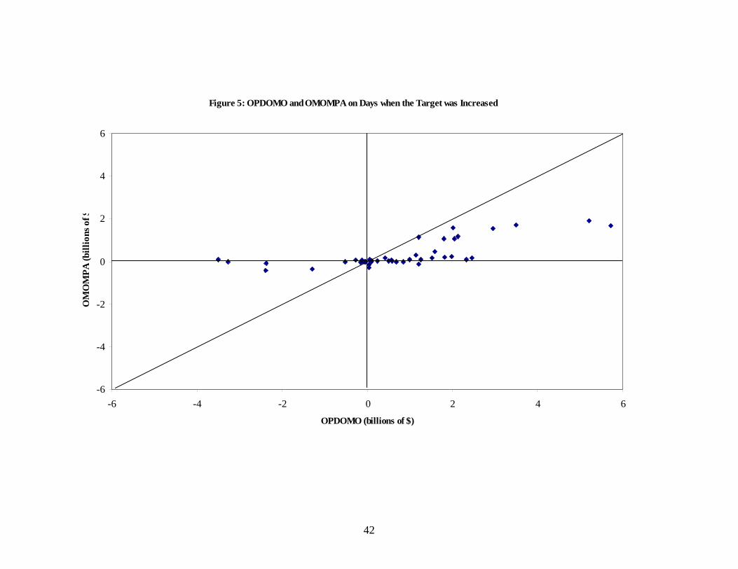
Figure 5: OPDOMO and OMOMPA on Days when the Target was Increased

-6

-4

-2

0

2

4

6

-6 -4 -2 0 2 4 6

OPDOMO (billions of $)

OM

OM

PA (b

illio

ns o

f $

42

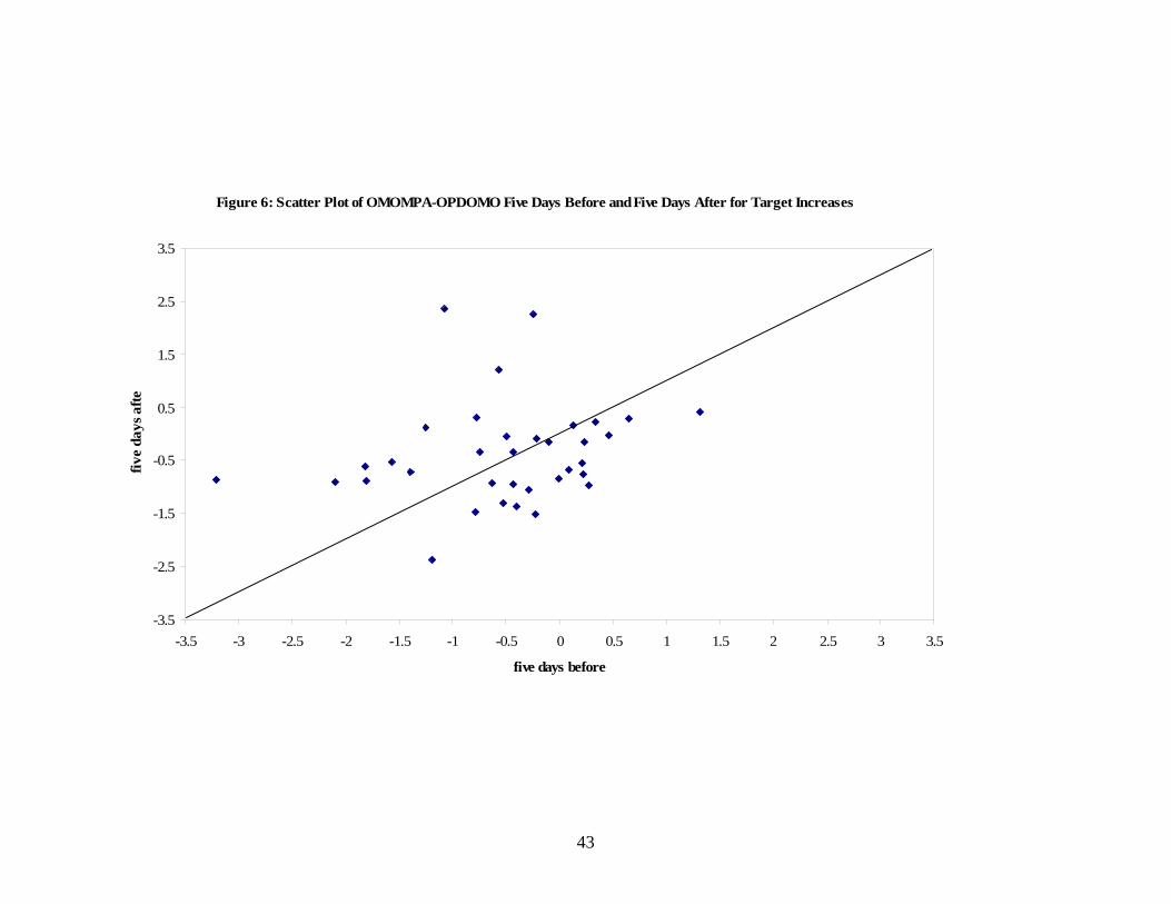
Figure 6: Scatter Plot of OMOMPA-OPDOMO Five Days Before and Five Days After for Target Increases

-3.5

-2.5

-1.5

-0.5

0.5

1.5

2.5

3.5

-3.5 -3 -2.5 -2 -1.5 -1 -0.5 0 0.5 1 1.5 2 2.5 3 3.5

five days before

five

days

afte

43

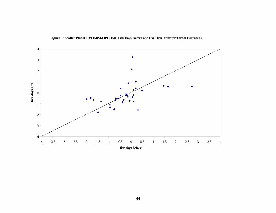
Figure 7: Scatter Plot of OMOMPA-OPDOMO Five Days Before and Five Days After for Target Decreases

-4

-3

-2

-1

0

1

2

3

4

-4 -3.5 -3 -2.5 -2 -1.5 -1 -0.5 0 0.5 1 1.5 2 2.5 3 3.5 4

five days before

five

days

afte

44

Figure 8: Scatter Plot of ff -fftar and Errors in forecasting Autonomous Factors(January 2, 1986 - December 31, 1996)

-8

-6

-4

-2

0

2

4

6

8

10

12

-2 -1 0 1 2 3 4

ff -fftar

fore

cast

err

or (b

illio

ns o

f $)

45

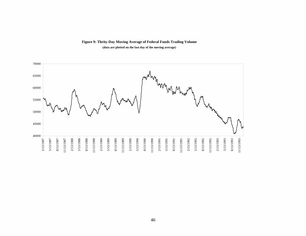
Figure 9: Thrity-Day Moving Average of Federal Funds Trading Volume(data are plotted on the last day of the moving average)

40000

45000

50000

55000

60000

65000

70000

2/13

/198

7

5/13

/198

7

8/13

/198

7

11/1

3/19

87

2/13

/198

8

5/13

/198

8

8/13

/198

8

11/1

3/19

88

2/13

/198

9

5/13

/198

9

8/13

/198

9

11/1

3/19

89

2/13

/199

0

5/13

/199

0

8/13

/199

0

11/1

3/19

90

2/13

/199

1

5/13

/199

1

8/13

/199

1

11/1

3/19

91

2/13

/199

2

5/13

/199

2

8/13

/199

2

11/1

3/19

92

2/13

/199

3

5/13

/199

3

8/13

/199

3

11/1

3/19

93

46