analysis of the impact of federal funds rate change on us ... · sesug 2015 1 paper bf-181 analysis...
TRANSCRIPT

SESUG 2015
1
Paper BF-181
Analysis of the Impact of Federal Funds Rate Change on US Treasuries Returns using SAS
Svetlana Gavrilova, Middle Tennessee State University; Maxim Terekhov, Vanderbilt University
ABSTRACT This paper analyzes the impact of federal funds rate changes on government bond returns and return volatility and compares it with equities market reaction. The purpose of this work is to construct a model estimating an expected risk exposure at a hypothetical point of time in the future given a description of current market conditions and historically observed events, which can be helpful in explaining expected movements and predicting future bond prices and volatility to use by portfolio managers in choosing asset allocation. We identify to which extent there is an impact of rate changes and the length of its effects. For our analysis we use data on major government bond prices and major macroeconomic characteristics of the U.S. economy between February 1990 and June 2015, collected on a daily basis. We model and forecast expected returns using ARIMA modeling based on different scenarios. Vector Autoregression and Vector Error Correction modeling is applied to estimate the impact of rate changes on government bonds performance and volatility. Credit markets behavior is compared to the equities market reaction. Findings are consistent with the previously published papers. US treasuries positively react on Federal Funds rate change, while equities market demonstrates a negative reaction. Long-term relationship between US Treasuries markets and Federal Funds rate is identified. The fact that a change in US treasuries market may be Granger caused by a change in Federal Funds target rate is statistically proved. All estimations are performed using SAS software.1
INTRODUCTION Financial markets are sensitive to many factors, including various macroeconomic parameters and policy changes (Ekanayake et al, 2008). Markets tend to react different on positive and negative events, as well as on difference between expectations and actual events. Investors are interested in predicting future market movements to optimize investment decisions under different scenarios. Professionals generate expectations based on their best guesses, technical and fundamental analysis, and multiple predictive models, creating a full overview based on different scenarios to make the best possible decisions.
Various policy changes are among the most influential factors impacting financial markets (Rigobon et al, 2002, Ekanayake et al, 2008). Federal Reserve regulates the US economy through monetary policy using Federal Funds target rate as a major influential instrument. Federal Open Market Committee (FOMC) is in charge of United States national monetary policy and oversees the nation’s open market operations. FOMC makes decisions regarding changes in Federal Funds Target Rate (FDTR) during regular meetings based on current economic conditions and future economic expectations. Typically an increase or a decrease in FDTR pulls equities and credit markets in different directions depending on other economic factors (Rigobon et al, 2002, Ekanayake et al, 2008) and preceding expectations (Bernanke et al, 2005). These facts increase interest for predicting FDTR impact on financial markets, and constantly stimulate demand for better models with higher predictive power.
Monetary policy is affecting all financial entities and activities in different ways. Theoretical finance assumes a positive relation between credit market returns and negative correlation between federal funds target rate and equity market returns. This may be explained by the fact that newly issued bonds tend to have higher coupon rates when issued later on an increase FDTR rate regime. This makes previously issued bonds less attractive for investors and therefore reduces the price during the secondary markets trading. This leads to an increase in returns to investors, who can now buy the bonds at lower price and still have the same coupon payments. All these changes are reflected in bond yields, calculated as a ration of a coupon to a current market price of security. A change in bond yields can be considered an approximation of returns on investment. Stock markets returns are represented by change in stocks prices as well as dividends paid. An increase in FDTR means an increase in cost of financing for companies, which may cause a decrease in their profits, and therefore dividends paid to shareholders. Also expectations regarding a potential decrease in profits and dividends may lead to a decrease in equity market price. This is the way finance explains expectations of a negative impact of equities markets on an increase in FDTR.
The question of FDTR increase is on the FOMC agenda again after years of no change. Market participants expect a potential increase announcement later in 2015 or early 2016. The abovementioned fact makes this paper relevant
1 JEL classification codes: G11, G12, G17, C32, C87. Keywords: Bond Yields, Stock Returns, Risk Analysis, Forecasting, SAS, Time Series Modeling, ARIMA, VAR, VECM, Cointegrtion, Causality.
2 For variables available on a quarterly basis we impute the latest available numbers for each day when no
Forecasting the Impact of Federal Fund Rate Change on US Treasuries Returns and Returns Volatility using SAS, continued SESUG 2015
2
and up to date with the current economic situation, since it estimates expected changes due to FDTR rise based on current economic conditions.
LITERATURE REVIEW Two major ways for statistical analysis applied to financial markets include historical analysis and stochastic approach. Both are widely described in numerous papers. Both ways may be used together or preference may be given to any type of analysis. In this paper we focus on time series analysis for financial forecasting based on historically observed data.
Autoregressive integrated moving average (ARIMA), vector autoregressive models (VAR), general autoregressive conditional heteroskedasticity models (GARCH) and various others are the widely accepted time series analysis modeling technique. ARIMA models were described by Box and Jenkins in 1970 and still hold one of superior places in financial forecasting allowing to produce models with good fit and generate precise short-term forecasts. Advantages of VAR models include incorporation of dynamically changing regressors (Zellner, 1962). They are widely used as an analytical tool, which makes possible to describe the interdependence mechanism between variables. GARCH models, introduced by Engle (1982), allow estimating conditional volatility, which can represent expected investment risks. Multivariate GARCH models (MGARCH), which allow to estimate various shocks impact on volatility were proposed by Harvey et al in 1994. Other models like neural networks and state-space models allow for latent variables and processes and may include elements of simulation, which stands them in between two major analysis flows.
Abovementioned models can be utilized for both equities and credit markets (Ekanayake et al, 2008). The two markets may react different on various shocks, so different quantitative models may work better for analysis of stocks and bonds. Time series analysis is more often used for analysis of equities market, while credit markets are in general more quantitatively complex and less analyzed by the time-series approach. We use time-series analysis for predicting markets movements, which is less common for credit markets. By applying time-series models we demonstrate how to create and use another helpful analytical tool, which allows to better understand market movements.
Federal funds rate change impact on equities markets is comprehensively analyzed, while credit markets related literature has a few time series analysis application papers published so far. Many authors are focused on an event – study framework, identifying impact of a change in FDTR on different classes of assets. Most of them do not implement out of sample forecasts. They also try to identify expected and unexpected portions of FDTR change onto financial markets (Bernanke et al, 2005; Hakan et al, 2010, Yin et al, 2010; Hsing, 2007). Both Bernanke and Hakan prove that unanticipated portion of FDTR change is influential, once an expected change does not lead to a significant markets reaction, while Hsing proves a decline of such an impact with an increase in maturity. Bernanke et al (2005) find a hypothetical 25 basic point increase in FDTR leads to a 1% increase in broad stock indexes. Ekanayake et al (2008) prove federal funds rate increase on average causes a negative reaction of stock markets, and a decrease in federal funds target rate positively affects stock markets. Friedman (1982) brings, that an increased volatility of a target rate leads to a decrease in external funding of corporations, increases bond yield spreads, and potentially change portfolio choice strategies for bond markets. Nishiyama’s findings support this idea with proving the causality relationship between long-term bond yields and the FDTR in 2007.
Federal funds target rate change is also justified to impact returns volatility (Bernanke et al, 1999; Bomfim, 2003, Bera et al, 1993). Chulia et al (2010) concludes the negative surprises trigger a bigger reaction in stock prices than positive ones. They also predict a 48 basis points increase in stock volatility during the first hour after the rate change announcement. Gospodinov et al (2012) validates the findings of other authors showing a bigger reaction of asset prices on unexpected changes while the expected component and general change is not causing a significant volatility transformation. Bollerslev et al (2000) findings verify the idea of a significant impact of macroeconomic announcements on credit markets volatility.
Many authors (Adebiyi et al, 2014, Mondal et al, 2014) find ARIMA modeling efficient in out-of-sample forecasting returns in the short-run. Others widely use VAR modeling to express an impact of FDTR change and its unexpected portion impact of financial markets (Bernanke et al, 2005; Hsing et al 2004; Kim et al, 2000). GARCH models are used to predict a change in volatility caused by total and unexpected FDTR changes (Chulia et al, 2009). In current world realities analytics complexity increases, requiring involvement of larger number of parameters and greater quantitative power. Big data analysis needs more efficient algorithms and relies on complex models, which also require powerful statistical software. There is a number of statistical software and packages that allow utilizing time series methodologies with ease. Numerous successful attempts to create a working forecasting system concentrated on particular tasks using SAS are made (Ratnaraj, 1995; Tangedal, 2003 Soriano et al, 2002; Gharibvand et al, 2010; Zlupko, 2009). In this paper we show how to build a useful forecasting system and analyze various factors impact using SAS.

Forecasting the Impact of Federal Fund Rate Change on US Treasuries Returns and Returns Volatility using SAS, continued SESUG 2015
3
DATA Data from Bloomberg Financial are used for this paper. We are interested in absolute changes in bond yields. We add data on equities markets represented by S&P500 index to compare the behavior of stock and bond markets under the FDTR change shock. We also use data on major macroeconomic variables extracted from Bloomberg, including consumer expenditures (PCE), new privately housing unit starts, unemployment rate, and M2 money velocity. Consumer expenditures, new housing starts and unemployment rate are very important economy characteristics indicating an economic cycle stage and overall economic health and are taken into consideration by many authors (Bernanke et al, 2005; Ekanayake et al, Haiyan, 2010). They also impact FOMC decisions regarding changes in monetary policy (Tylor, 1993; Mandler, 2012; Malliaris et al, 2009). M2 money velocity is a result of macroeconomic conditions and monetary policy and is considered an informative measure of population and business investment activity. Investors have a choice of classes of assets to choose for their portfolios. They prefer some assets to other ones and create a quasi-competition among assets. Thus, returns on one class of assets impact demand and, therefore, price and returns on other classes of assets (Bernanke, 2003). To acount for such effects we include most competing asset classes as explanatory variables in our models. We are interested in each class of US Government bond returns, which are expected to be influenced by other US government bond classes as well as equities markets and macroeconomic factors. Thus we also use equities market characteristics (S&P500) and oil prices (for Brent) as additional indicators. We restrict a potential impact by the abovementioned parameters for our model purposes. We download data on major categories of US government bonds for a period from February 1990 to June 2015 on a daily basis. For these data available with smaller frequency (FDTR, PCE, Unemployement, Housing starts, and M2 money velocity) we impute the level figures equal to the last information available, since market participants use these levels as a description of current economic conditions. All US treasuries data and FDTR data are used in a basic points scale, and housing starts are transformed by taking a log to maintain the comparable scale. All other variables are used on their real levels. Data covers a period of more than 25 years with many situational changes during this time frame. Initial data are non-stationary, so we use first differencing to reach stationarity. We also consider a potential structural break in our data, since the observed period covers the financial crisis of 2007. On the one hand, we speculate that this event may be treated as another “black swan”, creating outliers. On the other hand, crisis time covers relatively wide time period, which makes data behavior different from common outliers. To account for that and to estimate an impact of crisis we performed Chow test for a structural break for each of our models, and found no structural break which make implying further restrictions on a sample not necessary. The detailed results of the test are disclosed in the estimation results section.
Two different approaches are used for federal funds rate changes impact on financial markets. General approach (Kishor et al, 2013; Yin et al, 2010; Young et al, 2012) assumes that changes in level Federal Funds rate impact financial markets. We use pure federal funds rates to utilize this approach. Another theory assumes that only unexpected changes in FDTR impact financial markets, while expected changes do not cause any significant reaction (Bernanke et al, 2005; Berument et al, 2010, Hsing et al, 2004). Identifying unexpected changes is represented by two different methods in existing literature. The first one uses a change in federal funds rate futures rates to identify an expected portion of federal funds rate, and takes a difference between expected and real rate as unexpected part (Bernanke et al, 2005). The second one (Hsing et al, 2004) utilizes the difference between an effective federal funds rate (EFFR) changes and FDTR changes, as EFFR may be considered a measure of market expectations. For the purposes of this paper we use pure FDTR changes and unexpected changes based on EFFR approaches.
THE LIST OF VARIABLES
• GT2 – 2-year US government bond yields.
• GT5 – 5-year US government bond yields.
• GT10 – 10-year US government bond yields.
• GT30 – 30-year US government bond yields.
• SPX – S&P500 Index.
• FDTR – federal funds target rate.
• dFDTR – First difference in FDTR
• EFFR – Effective federal funds rate.
• dEFFR – First difference in EFFR
• unexpFR – Unexpected part of the federal funds rate as difference between Effective tax rate and FDTR.
• BRENT – Oil price (Brent).
Forecasting the Impact of Federal Fund Rate Change on US Treasuries Returns and Returns Volatility using SAS, continued SESUG 2015
4
• M2VEL – M2 money velocity2.
• UNEMPL – US Unemployment rate actual.
• HOUS – latest new housing starts.
• PCE - latest new housing starts.
The descriptive statistics for all variables is shown in Table 1.
METHODOLOGY We are interested in analyzing reaction of GT2, GT5, GT10, and GT30 on a change in FDTR. We also analyze SPX reaction on FDTR change to find out if equities and credit markets react differently. We apply ARIMA, VAR, and VECM modeling to estimate markets reaction. Each model specification and identification processes are presented below.
DATA PREPARATION AND TESTING
Level data for the given time series are not stationary in mean and variance, which can be identified by performing graphical analysis (see Figures 1 to 7 for details). First differencing is used to achieve data stationarity before running ARIMA and VAR models. A stationary time series is one whose statistical properties such as mean, variance, autocorrelation, etc. are all constant over time. The first difference of a time series is the series of changes from one period to the next. If Yt denotes the value of the time series Y at period t, then the first difference of Y at period t is equal to Yt-Yt-1. The autocorrelations decrease rapidly as reflected in the diagnostics plots (see Figures 1 to 7 for details), indicating a stationary time series.
We use the Augmented Dickey–Fuller test (ADF) to further test for a unit root in a time series sample (please, see Table 2 for sample output). It is an augmented version of the Dickey–Fuller test for a larger and more complicated set of time series models. Kwiatkowski–Phillips–Schmidt–Shin (KPSS) tests are used for testing a null hypothesis that an observable time series is stationary around a deterministic trend (see Table 3 for sample output). Based on the p-values of the ADF and KPSS tests we conclude that the time series is stationary (see Tables 4 for both tests result summary).
ARIMA
Autoregressive integrated moving average (ARIMA) model is a generalization of an autoregressive moving average (ARMA) model. ARIMA models are generally denoted as ARIMA (p, d, q), where parameters p, d, and q are non-negative integers: p is the order of the autoregressive model, d is the degree of differencing, and q is the order of the moving-average model. We run ARIMA to model the behavior for each of GT2, GT5, GT10, GT30, and SPX. Total 12 models for each outcome variable are performed and reviewed to identify a model that provides the best fit: 6 models to quantify the effect of FDTR and another 6 models to quantify the effect of unexpected rate change on each of the outcomes.
We run ARIMA model using (proc arima) for each of the outcome variables. Optimal lags are chosen by correlograms (plot of ACF and PACF versus Lag), goodness of fit criteria (Akaike Information Criteria (AIC), and standard errors estimate. All models correlogram and statistical results are consistent leading to a single true model choice. (Tables 5, 7, 10, 12, 15, 17, 20, 22, 24, and 27 represent the selection process for each asset consecutively).
For all GT2 bond yields ARIMA (1,1,2) model is chosen based on the abovementioned criteria with most for both methods (see Figure 1 for graphs). For GT5, GT10, GT30, and SPX ARIMA (2,1,3) provides best fit based on the abovementioned criteria for both methods (see Figures 2,3,4,7 for graphs). All Chow tests (Tables 9, 14, 19, 26, and 29) represent no structural break at the beginning (February 2007) and end (March 2009).
To estimate an impact of FDTR change on various classes of assets we create an out-of-sample set of observation, where all macroeconomic variables are given no change, financial market variables other than the output variable in each model are predicted by ARIMA, and FDTR and its unexpected portion are given a change of 25 basis points. Such an approach should help in estimating an impact of FDTR change since it allows isolating a change virtually to make it a virtually conducted experiment.
2 For variables available on a quarterly basis we impute the latest available numbers for each day when no announcements were made. Typically new data are issued at a particular date or at the last date of a calendar month, so the approach used allows us to catch up changes on a timely manner.
Forecasting the Impact of Federal Fund Rate Change on US Treasuries Returns and Returns Volatility using SAS, continued SESUG 2015
5
VAR AND VECM
We run VAR model using (proc varmax) for each of the outcome variables. We consider all asset types, and federal funds rate, since asset prices in general impact each other by participating in daily trades. All macroeconomic parameters and the oil price are considered as exogenous, since they impact financial markets and FDTR, but are not directly impacted by them. We assume that the latter parameters represent the US economy situation, creating conditions for financial markets movements, and so they should be included into the model. Optimal lag 2 is chosen based on the Hannan-Quinn (HQC) and Akaike Information Criteria (AIC) (see Table 30 for details) and subsequent models testing.
VAR model is primarily used for identification of FDTR and it unexpected portion impact on financial markets returns. Since we want to catch up the returns, monthly data are constructed by taking the latest available numbers for each calendar month for all variables. We use the first differences to obtain changes and returns and make data stationary.
VAR model is performed on differenced variables, since level variables are non-stationary. Strong VAR statistics witnesses a strong short run relationship between included variables. Our primary interest in the model is in estimating impulse response to a shock in FDTR identifying an impact of possible changes of one standard deviation. An uncorrelated time series can still be serially dependent due to a dynamic conditional variance process. A time series exhibiting conditional heteroscedasticity, or autocorrelation in the squared series, is said to have autoregressive conditional heteroscedastic (ARCH) effects (see Table 31 for details). We perform Engle's ARCH test (p<0.0001) to assess the significance of ARCH effects and conclude that no ARCH effects are present.
Having level variables non-stationary, we assume a possibility of long-term relationship between variables as well. Long-term relationships are tested by cointegration tests and estimated by Vector Error Correction Model (VECM). We perform Johansen test for testing cointegration of several time series (see Table 32 for details). Both restricted and unrestricted test results show an existence of 5 cointegrating vectors, which indicates an existence of strong long-term relationship between model variables. We estimate the relationship by VECM model of rank 5 (proc varmax) (please see Table 33 for details). Granger causality test is performed to identify causal relationship between the explanatory variable and regressors.
ESTIMATION RESULTS AND FORECASTING In this section we represent the output for best modes fitted and explain the economic sense of estimates. This section also covers the analytical portion of results. We also show forecasts based on different modeling techniques.
FORECASTING RETURNS USING ARIMA MODELING
Table 34 represents the best model specifications for each case. Tables 6, 8,11,13, 16, 18, 21, 23, and 28 represents estimation results for each ARIMA model consecutively. We indicate that all asset classes returns, as well as unemployment, money velocity, oil prices, target rate, along with unexpected rate change are identified as significant predictors (p<0.05) of GT2. An effect of rate change is positive, which is consistent with theoretical assumptions and prior findings. There is no significant difference in impact between FDTR and unexpFR found. An impact of unexpected portion of rate change is smaller than an effect of level rate change, which is different from the majority of prior finding. We speculate that such a difference from prior papers published before the financial crisis can be caused by an impact of a long period with no change in rate and relatively small recent volatility in efficient rate.
Fitting ARIMA for GT5 and GT10 indicates that unemployment, money velocity, oil, PCE along with bond yields and SPX are identified as significant predictors (p<0.05). We find an impact of FDTR and its unexpected portion change statistically insignificant, decreasing with exclusion of expected portion of change and partially negative. An impact of unexpected portion of rate change on GT5 is smaller than the effect of level rate change, which is different from major prior finding. We assume that such a difference with prior papers published before the financial crisis can be caused by an impact of a long period with no changes in rate and relatively small recent volatility in efficient rate. An impact of unexpected portion of rate change on GT10 is bigger than an effect of level rate change, which is consistent with prior publications.
We indicate that all asset classes returns, as well as unemployment, money velocity, oil prices, target rate, along with unexpected rate change are identified as significant predictors (p<0.05) of GT30. There is no significant difference in impact between FDTR and unexpFR found. An impact of unexpected portion of rate change is smaller than an effect of level rate change, which is different from major prior finding. The estimation results show that Federal funds rate is always statistically significant and the scale rises when an unexpected portion is used as a regressor. This supports findings of other authors.
Based on the best ARIMA model for each scenario we forecast expected changes in each asset class returns a few periods ahead. Since no macroeconomic data changes are present for the out-of-sample observations, only a modeled FDTR shock should be identified. Figures 9-17 represent forecasts of expected changes in outcome variables due to change in FDTR and its unexpected portion versus no shock simulated samples based on different
Forecasting the Impact of Federal Fund Rate Change on US Treasuries Returns and Returns Volatility using SAS, continued SESUG 2015
6
ARIMA models. All graphs show only a short-term impact of a shock in FDTR. GT2, GT10, and GT 30 demonstrate a few basis point upward movement in yields change due to 25 basis points increase in FDTR, which approaches zero change over the following 2-3 days. Unexpected portion change itself brings less volatility in returns than the entire change. The same scale of change was artificially created and used. We use the latest available effective Federal Funds rate to estimate the unexpected portion.
VAR MODEL ESTIMATION RESULTS
VAR model is performed on differenced variables since level variables are non-stationary. This approach involves an economic concept of returns. We treat a change in variables as returns on investment on a daily and monthly basis consecutively. Strong model statistics supports the assumption of well-defined short-term integration of variables in the model. All roots found are close to zero, which indicates the model stability. We construct an impulse response function for each of the asset classes to identify a potential impact of FDTR shock on assets returns (see Figure 18 for details). Impulse response represents a change in a variable of interest caused by a one standard error change in explanatory variable. Based on VAR estimation results, 1 standard deviation change (4 basis points) causes an increase in US Treasuries volatility and leads to an increase in yield changes after 4-5 days after the shock. Equities market negatively reacts to an increase in FDTR change demonstrating about 5 basis points decrease in 5 days after the 4 basis points shock in FDTR. These findings, representing a short-term relationship, are consistent with prior findings.
Johansen cointegration test supports the idea of existence of long-term cointegration, which is consistent with prior publications. VECM model normalized for GT2 is estimated based on 5 integration vectors. Long-run parameter (beta) and adjustment coefficients (alpha) estimates are give in Table 33. Granger causality test (see Table 34) indicates that US Treasuries returns changes are Granger caused by changes in model variables within 95% confidence interval. SPX changes are Granger caused by changes of model explanatory variables at 90%.
CONCLUSION In this paper we analyze an impact of Federal Funds target rate change on US Treasuries markets returns. We apply various time series analysis methods to estimate potential changes in financial market returns in case FOMC makes a decision to increase FDTR on a few points. ARIMA, VAR, and VECM models are used to identify potential aftermath of such a rise. We apply different forecasting scenarios and prove a positive impact of an increase in FDTR on bonds markets and a negative impact on stock markets. Our findings are consistent with prior publications, but bring smaller scale changes predicted comparing to papers published before the financial crisis of 2007. We speculate that one of the reasons for such a change can be caused by the markets adaptation to a long period of historically low rates, and a gradual slow upward movement may be less influential than the same during more volatile time.
We represent a step-by-step methodology of creating and using time-series analytical tools for financial markets analysis. We further provide interpretation of the estimation results and user cases in current economic context. The code, output, and further details are provided in the Appendix.
REFERENCES Bera A.K., and M. L. Higgins. 1993. ARCH models: Properties, Estimation and Testing. Journal of Economic Surveys, 7: 305-366.
Bernanke B.S. 2003. Monetary Policy and the stock market: some empirical results. October 2 Banking and Finance Lecture, Widener University, Chester, PA.
Bernanke B.S., and M. Gertler. 1999. Monetary policy and asset price volatility. Federal Reserve Bank of Kansas City Economic Review: 17-51.
Bernanke B.S., and K.N. Kuttner. 2005. What explains the stock market’s reaction to Federal Reserve policy? The Journal of Finance, LX: 1221-1257.
Berument H., and N. B. Ceylan. 2010. The effect of anticipated and unanticipated Federal funds target rate changes on domestic interest rates: international evidence. International Review of Applied Financial Issues and Economics, 2: 328-340.
Bollerslev T., J. Cai, and F.M. Song. 2000. Focus, Intraday periodicity, long memory volatility, and macroeconomic announcement effects in the US Treasury bond market. Journal of Empirical Finance, 7: 37-55.
Bomfim A. 2003. Pre-announcement effects, news effects, and volatility: monetary policy and the stock market. Journal of Banking and Finance, 27: 133-151.
Chulia H., M. Martens, and Dick van Dijk. 2010. Asymmetric effects of Federal funds target rate changes on S&P100 stock returns, volatilities and correlations. Journal of Banking and Finance, 34: 834-839.

Forecasting the Impact of Federal Fund Rate Change on US Treasuries Returns and Returns Volatility using SAS, continued SESUG 2015
7
Cochrane J.H., and M. Piazzesi. 2002. The Fed and interest rates: a high frequency identification. American Economic Review Papers and Proceedings, 92: 90-101.
Davidson, J. E. H., D.F.Hendry, F. Srba, and J. S Yeo. 1978. Econometric modelling of the aggregate time-series relationship between consumers' expenditure and income in the United Kingdom. Economic Journal, 88: 661–692.
Engle R.F. 1982. Autoregressive conditional heteroscedasticity with estimates of the variance of U.K. inflation. Econometrics, 50: 987 – 1008.
Ekanayake, E. M., R. Rance, and M. Halkides. 2008. Effects of Federal Funds Target Rate Changes on Stock Prices. The International Journal of Business and Finance Research, 2: 13-29.
Friedman B.M. 1982. Federal Reserve Policy, Interest Rate Volatility, and the U.S. Capital Raising Mechanism. Journal of Money, Credit and Banking, 14: 21-745.
Gospodinov N., and I. Jamali. 2012. The effects of Federal funds rate surprises on S&P 500 volatility and volatility risk premium. Journal of Empirical Finance, 19: 497-510.
Gharibvand S., and L. Gharibvand. 2010. Financial analysis using SAS PROCs. SAS Global Forum, Statistics and Data Ananlysis.
Haiyan Y, J. Yang, and W.C. Handorf. 2010. State dependency of bank stock reaction to Federal Funds rate target changes. The Journal of Financial Research, XXXIII: 289-315.
Harvey, A.C., E. Ruiz, and N. Shephard. 1994. Multivariate stochastic variance models. Review of Economic Studies, 61: 247-264.
Hsing Y. 2007. Effects of the intended and unintended federal funds rates on the Treasury yield curve during the Greenspan era. Applied Financial Economics Letters, 3: 155-159.
Hsing Y., and Y. Chen. 2004. Impacts of Macroeconomic Policies and Financial Market Performance on Output in Singapore: A VAR approach. The Journal of Developing Areas, 37: 73-98.
Kishor, N. K., and H. A. Marfatia. 2013. Does Federal Funds futures rate contain information about the treasury bill rate? Applied Financial Economics, 23: 1311-1324.
Kuttner K. 2001. Monetary policy surprises and interest rates: evidence from the Fed funds futures market. Journal of Monetary Economics, 47: 523-544.
Mandler M. 2012. Decomposing Federal Funds rate forecast uncertainty using time-varying Taylor rules and real-time data. North American Journal of Economics and Finance, 23: 228-245.
Malliaris A. G., and M. Malliaris. 2009. Modeling Federal Funds rates: a comparison of four methodologies. Neural Computing and Applicaions, 18: 37-44.
Ratnaraj P.J. 1995. Be bullish with SAS: financial and investment analysis with ease. 20th SAS Users Group International Conference Proceedings.
Rigobon R, and B. Sack. 2002. The impact of monetary policy on asset prices. Finance and Economic Discussion Series, 4. Board of Governors of the Federal Reserve System.
Soriano L. 2002. Analyze the stock market using the SAS system. 27th SAS Users Group International Meeting, Data Warehouse and Interprise Solutions.
Tangedal M. 2003. Using SAS as a definitive tool in stock market analysis. Midwest SAS USERS Group Meeting, Statistics, Data Analysis, and Modeling.
Taylor J.B. 1993. Discretion versus policy rules in practice. Carnegie-Rochester Conference Series on Public Policy 39: 195–214.
Yin H., J. Yang, and W.C. Handorf. 2010. State dependency of bank stock reaction to Federal funds rate target changes. The Journal of Financial Research, XXXIII: 289-315.
Young Y., and F. Bacon. 2012. The federal open market committee and the Federal funds rate: a test of market efficiency. Academy of Banking Studies Journal, 11: 81-92.
Zellner A. 1962. An efficient method of estimating seemingly unrelated regressions and tests for aggregation bias. Journal of American Statistical Association, 57: 348-368.
Zlupko T. 2009. SAS in financial research: Embracing data. SAS Global Forum Posters. Paper 202-2009.
Forecasting the Impact of Federal Fund Rate Change on US Treasuries Returns and Returns Volatility using SAS, continued SESUG 2015
8
TABLES
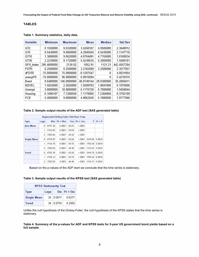
Table 1. Summary statistics, daily data.
Table 2. Sample output results of the ADF test (SAS generated table)
Based on the p-values of the ADF tesrt we conclude that the time series is stationary.
Table 3. Sample output results of the KPSS test (SAS generated table)
Unlike the null hypothesis of the Dickey-Fuller, the null hypothesis of the KPSS states that the time series is stationary
Table 4. Summary of the p-values for ADF and KPSS tests for 2-year US government bond yields based on a full sample.

Forecasting the Impact of Federal Fund Rate Change on US Treasuries Returns and Returns Volatility using SAS, continued SESUG 2015
9
VARIABLE (SAS) (First Difference)
ADF test p-value
KPSS test p-value
GT2 <0.0001 >0.05 GT5 <0.0001 >0.05 GT10 <0.0001 >0.05 GT30 <0.0001 >0.05 S&P500 <0.0001 >0.05 FDTR <0.0001 >0.05 unexpFR <0.0001 >0.05 BRENT <0.0001 >0.05 M2VEL <0.0001 >0.05 UNEMPL <0.0001 >0.05 HOUS <0.0001 >0.05
Table 5. Selection of the best ARIMA model based on the federal funds target rate for 2-year US government bond yields.
ARIMA AIC Std Error Estimate
(1,1,1) -43864.7 0.022724 (1,1,0) -43443.9 0.023247 (0,1,0) -42151.3 0.024926 (0,1,1) -43866.7 0.022723 (1,1,2)* -43870.6 0.022716 (2,1,0) -43859.1 0.022731
Lower values of AIC and standard error indicate better model fit. The asterisks above indicates the best (that is, minimized) values of the Akaike Information Criterion and Standard Error Estimate
Table 6. Maximum likelihood estimation details for ARIMA (1,1,2) fitting 2-year US government bond yields series based on the federal funds target rate (SAS generated table)

Forecasting the Impact of Federal Fund Rate Change on US Treasuries Returns and Returns Volatility using SAS, continued SESUG 2015
10
Table 7. Selection of the best ARIMA model based on the unexpected part of the federal funds rate for 2-year US government bond yields.
ARIMA AIC Std Error Estimate
(1,1,1) -43820.5 0.022778 (1,1,0) -43405.1 0.023296 (0,1,0) -42105.2 0.024988 (0,1,1) -43822.4 0.022777 (1,1,2)* -43824.1 0.022773 (2,1,0) -43810.7 0.02279
Lower values of AIC and standard error indicate better model fit. The asterisks above indicates the best (that is, minimized) values of the Akaike Information Criterion and Standard Error Estimate
Table 8. Maximum likelihood estimation details for ARIMA (1,1,2) fitting 2-year US government bond yields series based on the unexpected part of the federal funds rate (SAS generated table)

Forecasting the Impact of Federal Fund Rate Change on US Treasuries Returns and Returns Volatility using SAS, continued SESUG 2015
11
Table 9. Structural change (Chow) test results for 2-year US government bond yields series (SAS generated table)
Table 10. Selection of the best ARIMA model based on the target federal funds rate for 5-year US government bond yields.
ARIMA AIC Std Error Estimate
(1,1,1) -53104.5 0.013809 (1,1,0) -52691.7 0.014121 (0,1,0) -51587.3 0.014988 (0,1,1) -53103.1 0.013811 (1,1,2) -53124.3 0.013794 (2,1,3)* -53192.1 0.013742
Table 11. Maximum likelihood estimation details for ARIMA (2,1,3) fitting 5-year US government bond yields series based on the federal funds target rate (SAS generated table)
Forecasting the Impact of Federal Fund Rate Change on US Treasuries Returns and Returns Volatility using SAS, continued SESUG 2015
12
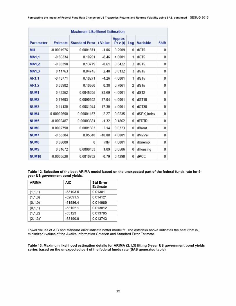
Table 12. Selection of the best ARIMA model based on the unexpected part of the federal funds rate for 5-year US government bond yields.
ARIMA AIC Std Error Estimate
(1,1,1) -53103.5 0.01381 (1,1,0) -52691.5 0.014121 (0,1,0) -51586.4 0.014989 (0,1,1) -53102.1 0.013812 (1,1,2) -53123 0.013795 (2,1,3)* -53190.9 0.013743
Lower values of AIC and standard error indicate better model fit. The asterisks above indicates the best (that is, minimized) values of the Akaike Information Criterion and Standard Error Estimate
Table 13. Maximum likelihood estimation details for ARIMA (2,1,3) fitting 5-year US government bond yields series based on the unexpected part of the federal funds rate (SAS generated table)

Forecasting the Impact of Federal Fund Rate Change on US Treasuries Returns and Returns Volatility using SAS, continued SESUG 2015
13
Table 14. Structural change (Chow) test results for 5-year US government bond yields series (SAS generated table)
Table 15. Selection of the best ARIMA model based on the federal funds target rate for 10-year US government bond yields.
ARIMA AIC Std Error Estimate
(1,1,1) -56061.6 0.011774 (1,1,0) -55543.3 0.012109 (0,1,0) -54112.9 0.01308 (0,1,1) -56061.9 0.011775 (1,1,2) -56069.4 0.011769 (2,1,3)* -56162.8 0.011708

Forecasting the Impact of Federal Fund Rate Change on US Treasuries Returns and Returns Volatility using SAS, continued SESUG 2015
14
Lower values of AIC and standard error indicate better model fit. The asterisks above indicates the best (that is, minimized) values of the Akaike Information Criterion and Standard Error Estimate
Table 16. Maximum likelihood estimation details for ARIMA (2,1,3) fitting 10-year US government bond yields series based on the federal funds target rate (SAS generated table)
Table 17. Selection of the best ARIMA model based on the unexpected part of the federal funds rate for 10-year US government bond yields.
ARIMA AIC Std Error Estimate
(1,1,1) -56061.2 0.011774 (1,1,0) -55543.7 0.012108 (0,1,0) -54115.2 0.013078 (0,1,1) -56061.6 0.011775 (1,1,2) -56069.2 0.011769 (2,1,3)* -56161.8 0.011709
Lower values of AIC and standard error indicate better model fit. The asterisks above indicates the best (that is, minimized) values of the Akaike Information Criterion and Standard Error Estimate
Table 18. Maximum likelihood estimation details for ARIMA (2,1,3) fitting 10-year US government bond yields series based on the unexpected part of the federal funds rate (SAS generated table)

Forecasting the Impact of Federal Fund Rate Change on US Treasuries Returns and Returns Volatility using SAS, continued SESUG 2015
15
Table 19. Structural change (Chow) test results for 10-year US government bond yields series (SAS generated table)
Table 20. Selection of the best ARIMA model based on the federal funds target rate for 30-year US government bond yields.
ARIMA AIC Std Error Estimate
(1,1,1) -49140.2 0.017099 (1,1,0) -48547.5 0.017655 (0,1,0) -46672.9 0.019534 (0,1,1) -49112.6 0.017126 (1,1,2) -49108.8 0.017127 (2,1,3)* -49230.8 0.017013

Forecasting the Impact of Federal Fund Rate Change on US Treasuries Returns and Returns Volatility using SAS, continued SESUG 2015
16
Lower values of AIC and standard error indicate better model fit. The asterisks above indicates the best (that is, minimized) values of the Akaike Information Criterion and Standard Error Estimate
Table 21. Maximum likelihood estimation details for ARIMA (2,1,3) fitting 30-year US government bond yields series based on the federal funds target rate (SAS generated table)
Table 22. Selection of the best ARIMA model based on the unexpected part of the federal funds rate for 30-year US government bond yields.
ARIMA AIC Std Error Estimate
(1,1,1) -49238.2 0.017006 (1,1,0) -48555.9 0.017647 (0,1,0) -46679.5 0.019527 (0,1,1) -49120.4 0.017118 (1,1,2) -49116.6 0.01712 (2,1,3)* -49238.2 0.017006
Lower values of AIC and standard error indicate better model fit. The asterisks above indicates the best (that is, minimized) values of the Akaike Information Criterion and Standard Error Estimate
Table 23. Maximum likelihood estimation details for ARIMA (2,1,0) fitting 30-year US government bond yields series based on the unexpected part of the federal funds rate (SAS generated table)

Forecasting the Impact of Federal Fund Rate Change on US Treasuries Returns and Returns Volatility using SAS, continued SESUG 2015
17
Table 24. Selection of the best ARIMA model based on the federal funds target rate for S&P500.
ARIMA AIC Std Error Estimate
(1,1,1) 72462.46 12.02127 (1,1,0) 72969.31 12.355 (0,1,0) 74639.56 13.51993 (0,1,1) 72473.33 12.02897 (1,1,2) 72405.31 11.98363 (2,1,3)* 72385.6 11.96961
Lower values of AIC and standard error indicate better model fit. The asterisks above indicates the best (that is, minimized) values of the Akaike Information Criterion and Standard Error Estimate
Table 25. Maximum likelihood estimation details for ARIMA (1,0,1) fitting S&P500 series based on the federal funds target rate (SAS generated table)

Forecasting the Impact of Federal Fund Rate Change on US Treasuries Returns and Returns Volatility using SAS, continued SESUG 2015
18
Table 26. Structural change (Chow) test results for 10-year US government bond yields series (SAS generated table)
Table 27. Selection of the best ARIMA model based on the unexpected part of the federal funds rate for S&P500.
ARIMA AIC Std Error Estimate
(1,1,1) 72469.26 12.02568 (1,1,0) 72976.9 12.36006 (0,1,0) 74644.98 13.52388 (0,1,1) 72479.98 12.03328 (1,1,2) 72412.02 11.98796 (2,1,3)* 72392.08 11.97379
Forecasting the Impact of Federal Fund Rate Change on US Treasuries Returns and Returns Volatility using SAS, continued SESUG 2015
19
Lower values of AIC and standard error indicate better model fit. The asterisks above indicates the best (that is, minimized) values of the Akaike Information Criterion and Standard Error Estimate
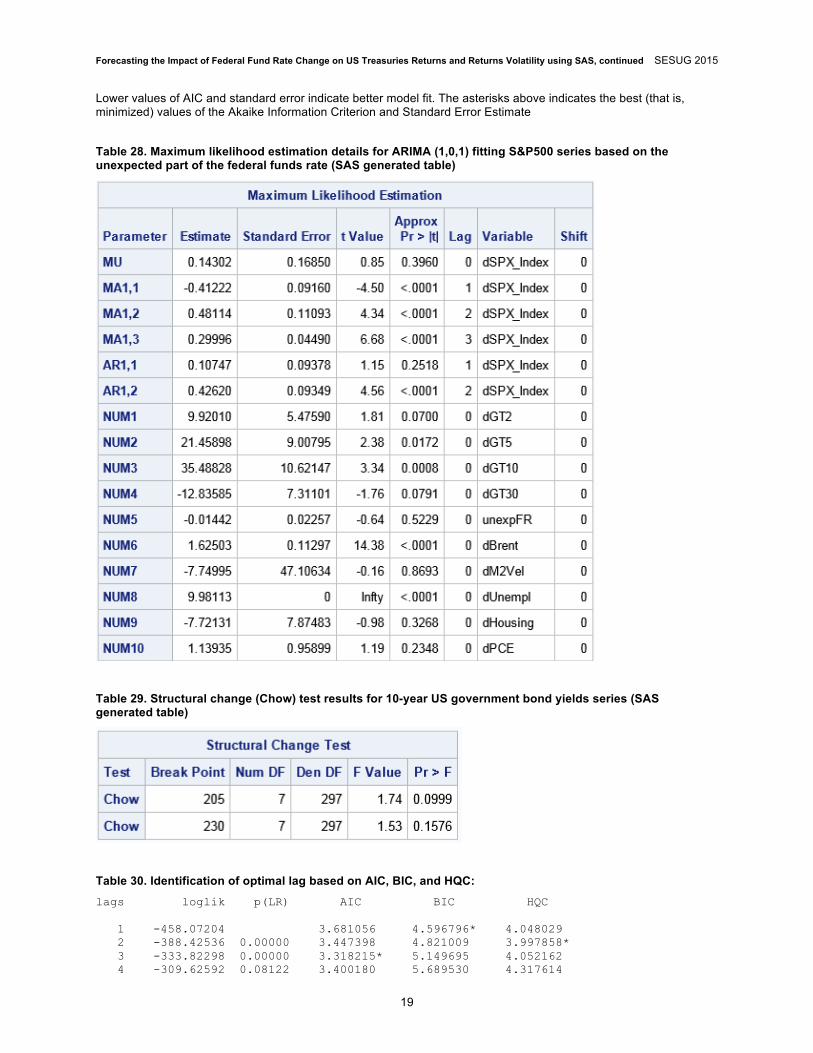
Table 28. Maximum likelihood estimation details for ARIMA (1,0,1) fitting S&P500 series based on the unexpected part of the federal funds rate (SAS generated table)
Table 29. Structural change (Chow) test results for 10-year US government bond yields series (SAS generated table)
Table 30. Identification of optimal lag based on AIC, BIC, and HQC: lags loglik p(LR) AIC BIC HQC 1 -458.07204 3.681056 4.596796* 4.048029 2 -388.42536 0.00000 3.447398 4.821009 3.997858* 3 -333.82298 0.00000 3.318215* 5.149695 4.052162 4 -309.62592 0.08122 3.400180 5.689530 4.317614
Forecasting the Impact of Federal Fund Rate Change on US Treasuries Returns and Returns Volatility using SAS, continued SESUG 2015
20
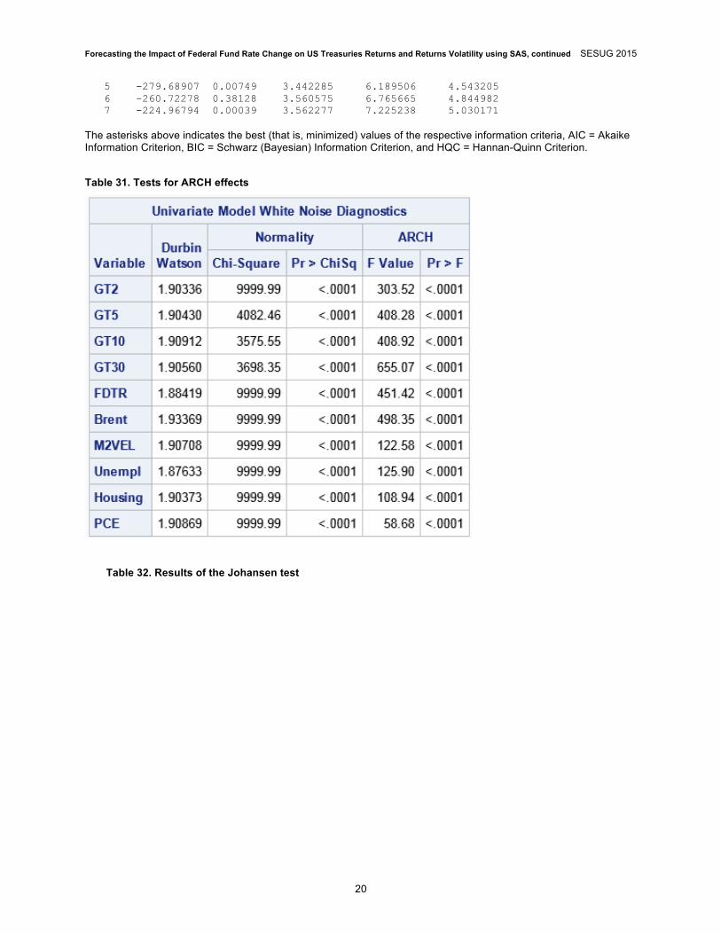
5 -279.68907 0.00749 3.442285 6.189506 4.543205 6 -260.72278 0.38128 3.560575 6.765665 4.844982 7 -224.96794 0.00039 3.562277 7.225238 5.030171 The asterisks above indicates the best (that is, minimized) values of the respective information criteria, AIC = Akaike Information Criterion, BIC = Schwarz (Bayesian) Information Criterion, and HQC = Hannan-Quinn Criterion.
Table 31. Tests for ARCH effects
Table 32. Results of the Johansen test

Forecasting the Impact of Federal Fund Rate Change on US Treasuries Returns and Returns Volatility using SAS, continued SESUG 2015
21
Table 33. VECM Coefficients and parameter estimates

Forecasting the Impact of Federal Fund Rate Change on US Treasuries Returns and Returns Volatility using SAS, continued SESUG 2015
22
Table 34. Granger causality test results
GRAPHS Figure 1. 2-year US government bond yields and its first difference, which converts non-stationary data to stationary:

Forecasting the Impact of Federal Fund Rate Change on US Treasuries Returns and Returns Volatility using SAS, continued SESUG 2015
23
Figure 2. 5-year US government bond yields and its first difference, which converts non-stationary data to stationary:
Figure 3. 10-year US government bond yields and its first difference, which converts non-stationary data to stationary:
Figure 4. 30-year US government bond yields and its first difference, which converts non-stationary data to stationary:
Figure 5. Federal funds target rate and its first difference, which converts non-stationary data to stationary:

Forecasting the Impact of Federal Fund Rate Change on US Treasuries Returns and Returns Volatility using SAS, continued SESUG 2015
24
Figure 6. Effective federal funds rate and its first difference, which converts non-stationary data to stationary:
Figure 7. SPX Index and its first difference, which converts non-stationary data to stationary:

Forecasting the Impact of Federal Fund Rate Change on US Treasuries Returns and Returns Volatility using SAS, continued SESUG 2015
25
Figure 8. Sample ARIMA diagnostics output and maximum likelihood estimators.
Figure 9. Prediction of S&P 500 without a shock in fed rate
Figure 10. Prediction of first difference in 2-year US government bond yields with and without a shock in federal funds target rate
Figure 11. Prediction of first difference in 2-year US government bond yields with and without a shock in the unexpected part of the federal funds rate

Forecasting the Impact of Federal Fund Rate Change on US Treasuries Returns and Returns Volatility using SAS, continued SESUG 2015
26
Figure 12. Prediction of first difference in 5-year US government bond yields with and without a shock in federal funds target rate
Figure 13. Prediction of first difference in 5-year US government bond yields with and without a shock in the unexpected part of the federal funds rate

Forecasting the Impact of Federal Fund Rate Change on US Treasuries Returns and Returns Volatility using SAS, continued SESUG 2015
27
Figure 14. Prediction of first difference in 10-year US government bond yields with and without a shock in federal funds target rate
Figure 15. Prediction of first difference in 10-year US government bond yields with and without a shock in the unexpected part of the federal funds rate
Figure 16. Prediction of first difference in 30-year US government bond yields with and without a shock in federal funds target rate

Forecasting the Impact of Federal Fund Rate Change on US Treasuries Returns and Returns Volatility using SAS, continued SESUG 2015
28
Figure 17. Prediction of first difference in 30-year US government bond yields with and without a shock in the unexpected part of the federal funds rate
Figure 18. Response to impulse in FDTR in different bond yields and SPX

Forecasting the Impact of Federal Fund Rate Change on US Treasuries Returns and Returns Volatility using SAS, continued SESUG 2015
29
CODES APPENDIX We create summary statistics using the following code:
proc means data = DataFullDayDif min max mean median std; var GT2 GT5 GT10 GT30 SPX FDTR EFFR unexpFR Brent M2Vel Unempl Housing PCE; run;
The autocorrelations decrease rapidly in this plot, indicating that the change in abovementioned variable is a stationary time series.
proc arima data=DataFullDayDif; identify var=GT2; run; proc arima data=DataFullDayDif; identify var=GT2(1); run;
Augmented-Dickey Fuller (ADF) and KPSS tests are used to test for stationarity:
proc arima data = DataFullDayDif; identify var=GT2(1) stationarity=(adf);
run;
Unlike the null hypothesis of the Dickey-Fuller, the null hypothesis of the KPSS states that the time series is stationary:
Forecasting the Impact of Federal Fund Rate Change on US Treasuries Returns and Returns Volatility using SAS, continued SESUG 2015
30
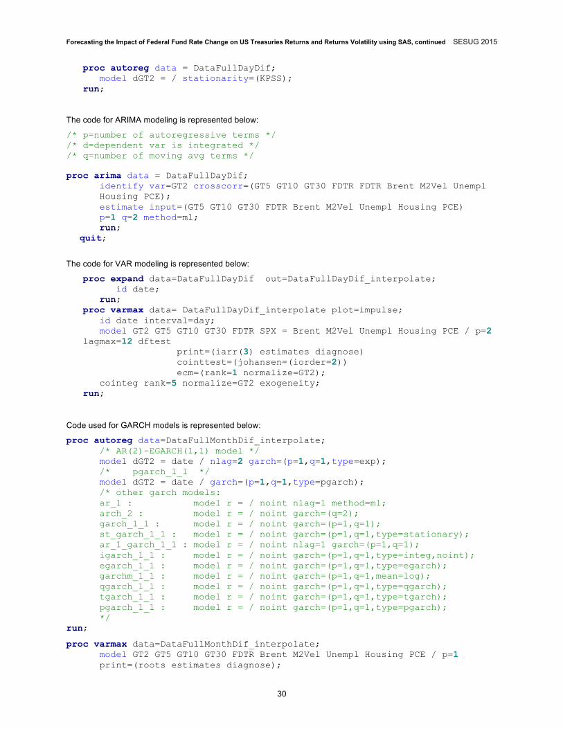
proc autoreg data = DataFullDayDif; model dGT2 = / stationarity=(KPSS);
run;
The code for ARIMA modeling is represented below:
/* p=number of autoregressive terms */ /* d=dependent var is integrated */ /* q=number of moving avg terms */ proc arima data = DataFullDayDif;
identify var=GT2 crosscorr=(GT5 GT10 GT30 FDTR FDTR Brent M2Vel Unempl Housing PCE); estimate input=(GT5 GT10 GT30 FDTR Brent M2Vel Unempl Housing PCE) p=1 q=2 method=ml; run;
quit;
The code for VAR modeling is represented below:
proc expand data=DataFullDayDif out=DataFullDayDif_interpolate; id date; run; proc varmax data= DataFullDayDif_interpolate plot=impulse; id date interval=day; model GT2 GT5 GT10 GT30 FDTR SPX = Brent M2Vel Unempl Housing PCE / p=2 lagmax=12 dftest print=(iarr(3) estimates diagnose) cointtest=(johansen=(iorder=2)) ecm=(rank=1 normalize=GT2); cointeg rank=5 normalize=GT2 exogeneity; run;
Code used for GARCH models is represented below:
proc autoreg data=DataFullMonthDif_interpolate; /* AR(2)-EGARCH(1,1) model */ model dGT2 = date / nlag=2 garch=(p=1,q=1,type=exp); /* pgarch_1_1 */ model dGT2 = date / garch=(p=1,q=1,type=pgarch); /* other garch models: ar_1 : model r = / noint nlag=1 method=ml; arch_2 : model r = / noint garch=(q=2); garch_1_1 : model r = / noint garch=(p=1,q=1); st_garch_1_1 : model r = / noint garch=(p=1,q=1,type=stationary); ar_1_garch_1_1 : model r = / noint nlag=1 garch=(p=1,q=1); igarch_1_1 : model r = / noint garch=(p=1,q=1,type=integ,noint); egarch_1_1 : model r = / noint garch=(p=1,q=1,type=egarch); garchm_1_1 : model r = / noint garch=(p=1,q=1,mean=log); qgarch_1_1 : model r = / noint garch=(p=1,q=1,type=qgarch); tgarch_1_1 : model r = / noint garch=(p=1,q=1,type=tgarch); pgarch_1_1 : model r = / noint garch=(p=1,q=1,type=pgarch); */ run;
proc varmax data=DataFullMonthDif_interpolate; model GT2 GT5 GT10 GT30 FDTR Brent M2Vel Unempl Housing PCE / p=1 print=(roots estimates diagnose);

Forecasting the Impact of Federal Fund Rate Change on US Treasuries Returns and Returns Volatility using SAS, continued SESUG 2015
31
garch p=1 q=2; nloptions tech=qn maxiter=500;
run;
CONTACT INFORMATION Your comments and questions are valued and encouraged. Contact the author at:
Svetlana Gavrilova Middle Tennessee State University 1301 East Main Street Murfreesboro, TN, 37132 [email protected] capone.mtsu.edu/sag4q Maxim Terekhov Vanderbilt University 1211 21st Ave S Medical Arts Building, #708 Nashville, TN, 37235 [email protected]
SAS and all other SAS Institute Inc. product or service names are registered trademarks or trademarks of SAS Institute Inc. in the USA and other countries. ® indicates USA registration.
Other brand and product names are trademarks of their respective companies.