On the Strategic Disclosure of FeasibleOptions in Bargaining

Geoffroy de Clippel∗ Kfir Eliaz†

October 2011

Abstract

Most of the economic literature on bargaining has focused on situations where theset of possible outcomes is taken as given. This paper is concerned with situationswhere decision-makers first need to identify the set of feasible outcomes before theybargain over which of them is selected. Our objective is to understand how differentbargaining institutions affect the incentives to disclose possible solutions to the bargain-ing problem, where inefficiency may arise when both parties withold Pareto superioroptions. We take a first step in this direction by proposing a simple, stylized modelthat captures the idea that bargainers may strategically withhold information regard-ing the existence of feasible alternatives that are Pareto superior. We characterize apartial ordering of “regular” bargaining solutions (i.e., those belonging to some classof “natural” solutions) according to the likelihood of disclosure that they induce. Thisordering identifies the best solution in this class, which favors the “weaker” bargainersubject to the regularity constraints. We also illustrate our result in a simple environ-ment where the best solution coincides with Nash, and where the Kalai-Smorodinskysolution is ranked above Raiffa’s simple coin-toss solution. The analysis is extended toa dynamic setting in which the bargainers can choose the timing of disclosure. Com-paring the static and dynamic games, we show that enforcing a hard deadline can bewelfare improving.

∗Department of Economics, Brown University. Email: declippel@brown.edu. Financial support from theDeutsche Bank through the Institute for Advanced Study is gratefully acknowledged.†Department of Economics, Brown University. Email: kfir eliaz@brown.edu

1

1. INTRODUCTION

Bargaining theory aims to understand how parties resolve conflicting interests on which

outcome to implement. The economic literature has focused so far on the case where the set

of feasible alternatives is obvious, e.g. the possible allocations of some monetary value. There

are, however, many situations where this set is not commonly known. In these situations,

the bargainers themselves must identify the feasible solutions to their conflict.

One common situation with these features is the selection of a candidate, or a group of

candidates, for a task by several parties with conflicting interests: deciding which candidate

to hire for a vacant post, choosing a candidate to run for office, deciding on the composition

of some external committee, choosing an arbitrator, etc. Quite often it is not commonly

known which potential candidates are suitable for the task, and which are actually willing to

be nominated. Hence, the parties responsible for making the decision must propose names

of qualified and available candidates from which a selection can be made. Another example

is that of international conflicts, where different parties may have conflicting interests on

say, how to address the development of a nuclear program by a hostile country, or how to

fight against terrorism or how to resolve an ethnic conflict. Possible solutions may involve

different forms of sanctions, a variety of military operations or the creation of new reforms

or laws. The parties who wish to resolve the conflict would need to identify concrete plans

of actions. Another, more mundane example, is that of a husband and a wife, who need to

decide which house to buy, or which city/state/country to move to, or which school to send

their kids to. Both sides need to identify feasible alternatives (e.g., which houses are for sale,

which locations have relevant job openings, which schools have open slots), and the two may

have conflicting interests regarding the choice (e.g., each may want a house closer to his/her

workplace, each may want to move to a location with better career opportunities or closer

to one’s family, each may have a different preference on public versus private education).

Such conflicts of interests have received much attention in the more applied or popular

literature (see e.g. Fisher et al. (1991), or the webpage of the Federal Mediation and

Conciliation Service). For example, one of the key steps in what is known as interest-based

(or integrative, or win-win, or mutual gains, or principled) bargaining technique is for both

parties to suggest feasible options, before implementing an agreed-upon objective criterion

(e.g. “traditional practices,” “what a court would decide,” “comparing the options’ market

value,” “fairness,” etc.) to evaluate them. However, private incentives may go against the

systematic disclosure of “win-win” options: rational parties would anticipate what is the

potential impact on the final outcome of disclosing an option. Thus, even if a party is aware

of an alternative that is Pareto improving, it may decide to withhold that information in

the hope that another party will reveal a more profitable option that it is not aware of. The

2

popular literature on negotiations suggests that such strategic concerns are real and may

impede negotiations. For instance, the disputing parties are instructed to suggest as rapidly

as possible (which may be interpreted as a way to limit strategic considerations), a number of

solutions that might meet the needs of the parties. It is often emphasized that evaluating the

proposed options is irrelevant at this stage, as selection will occur only after a satisfactory

number of options have been proposed or the parties have exhausted their ideas.1

While classical bargaining theory has taken the set of feasible agreements as an exoge-

nous variable,2 this paper explores how this set emerges endogenously. In particular, our

objective is to understand how different bargaining institutions affect the incentives to dis-

close possible solutions to the bargaining problem, where inefficiency may arise when both

parties withold Pareto superior options. We take a first step in this direction by proposing

a simple, stylized model that captures the idea that bargainers may strategically withhold

information regarding the existence of feasible alternatives that are Pareto superior. Section

2 presents our basic model, which investigates the case where each bargainer knows only

about one feasible solution to the bargaining, and his decision problem is whether or not to

disclose his information. More specifically, there are two bargainers, who each has learned

(in the sense of obtaining verifiable evidence) about the feasibility of some option. Neither

bargainer knows what option the other has learned about, but they both have a common

prior on the payoffs associated with the potentially feasible options. The bargainers first de-

cide (simultaneously) whether or not to disclose their options, and then in the second stage,

they apply a bargaining solution, which is modeled as a function that assigns to every set of

disclosed options a lottery on the union of this set and the disagreement point. Attention is

restricted to a class of bargaining solutions (referred to as “regular”) with some reasonable

properties, which in our basic set-up contains all the classical solutions such as Raiffa, Kalai-

Smorodinsky and Nash. We interpret the “regularity” properties of a bargaining solution as

“descriptive” properties in the sense that parties to a dispute would want to use bargaining

procedures that possess these properties (they may be viewed as “normative” properties

when one takes the set of agreements as given). We emphasize that our model abstracts

from many details that accompany real-life negotiations (such as those described above) and

1One vivid example of this appears in Haynes (1986), who discusses the role of mediators when imple-menting an interest-based approach to divorce and family issues: “If the mediator determines that the partiesare withholding options with a covert strategy in mind, the mediator can cite a similar situation with anothercouple and describe different options they considered. This can helps break the logjam by forcing the coupleto examine the options and including them on their list, thereby creating a greater level of safety for otheroptions that are developed after one goes up on the board.” In our model, though, feasible options can onlybe disclosed by the bargainers themselves - there will be no mediator with extra information to break thelogjam.

2Two notable exceptions are Kalai and Samet (1985) and Frankel (1998), a discussion of which is includedin Section 7.

3

may fit some situations better than others. Its purpose is not to give a one-to-one mapping

of reality but rather, to provide a tractable framework that enables us to isolate the effect

of the bargaining procedure on the incentives to disclose feasible options.

Focusing on the symmetric Bayesian Nash equilibria of the disclosure game, we show

in Section 3 that each bargaining solution induces a unique, strictly positive, probability

of no-disclosure (and hence, disagreement). This probability uniquely determines the ex-

ante welfare of the bargainers in our model. In Section 4, we define a partial ordering

on regular bargaining solutions, and show that being superior according to that ordering

implies a higher degree of efficiency in the symmetric equilibrium of the disclosure game.

In the simple environment we begin with, this partial ordering implies that the level of

inefficiency is systematically lower when the Nash solution is applied than when the Kalai-

Smorodinsky solution is applied, and in turn lower than when the Raiffa solution is applied.

Moreover, in this environment the Nash solution induces the minimal level of inefficiency

among all regular solutions. As a dual result, we also derive an upper-bound on the level of

inefficiency that is possible when picking the final option according to a regular bargaining

solution. In addition, we show that our partial ordering induces a lattice structure on the

set of regular bargaining solutions: given any pair of regular solutions, we can construct a

new pair of regular solutions, one which is more efficient than each of the original solutions,

and another, which is less efficient.

When evaluating the efficiency of bargaining solutions, our approach is to take as given

the set of solutions that are used (with the interpretation that most disputes are resolved

via some regular bargaining solution), and ask which procedures perform better in terms of

disclosure. An analagous approach is taken in the literature that examines the incentives

to engage in costly information acquisition under different committee designs or under dif-

ferent auction formats (see Persico (2000, 2004)). An alternative, implementation-theoretic

approach, which is not taken in this paper, is to try and internalize the incentive to disclose

information by designing an optimal mechanism that assigns to every pair of bargainer types

a probability of disclosure and a probability distribution over the feasible outcomes.3

Inefficiency in the disclosure game occurs when both parties withhold their information.

One may wonder then, why neither of them reacts before having to settle down with the

disagreement outcome, since both are aware of Pareto improving options. While letting bar-

gainers do this may seem beneficial at first, having an opportunity to speak in a subsequent

stage also diminishes one’s incentive to speak right away. We address the question of dis-

3To illustrate the difference betwen these two approaches, compare Persico (2004) that studies the incen-tives to acquire information under prevalent committee designs (specifically, threshold voting rules), withGerardi and Yariv (2008) that characterize the ex-ante optimal collective decision-making procedure.

4

closure over time, where pure inefficiency now becomes a delay. In equilibrium, a bargainer

immediately discloses an option if it is relatively favorable to him, and will delay disclosure

for less favorable options, where the rate of delay is independent of the bargaining solution.

However, the likelihood of disclosing immediately varies with the solution, and it turns out

that the normative comparison derived for the one-shot game carries over to the dynamic

game: delay is uniformly lower if the solution that is applied is larger according to the in-

complete ordering defined in Section 4, and the Nash solution is thus optimal if the objective

is to minimize the level of inefficiency. While in general, we cannot compare the bargainers’

welfare in the static and dynamic game, we show that for a uniform distribution of bargainer

types, the ex-ante expected welfare under the Raiffa, Nash and Kalai-Smorodinsly solutions

are strictly lower in the dynamic game than in the static game. Hence committing to a

hard deadline that forces the parties to speak at once, and to overlook any subesequent

disclosure, may be preferable. We conclude Section 5 by examining a variant of the dynamic

disclosure game where bargainers have the possibility to react immediately after the other

had disclosed his option, i.e. before the bargaining solution is applied. In that case, the

equilibrium probability of immediate disclosure is independent of the bargaining solution.

Furthermore, for every regular bargaining solution and for every bargainer type, the timing

of disclosure is delayed relative to the original dynamic disclosure game.

Section 6 extends the analysis of the static game to a more general environment, where

we characterize the most efficient regular bargaining solution (which reduces to the Nash

solution in the simple emvironment of Section 2). This solution has the property that

whenever two options have been disclosed, it seeks to maximize the expected payoff of the

“weaker” bargainer (in the sense that his minimal payoff from the two disclosed options is

lower than the minimal payoff of the other bargainer) subject to the constraint that the

stronger bargainer obtains as close as possible to half of the maximal attainable surplus.

Section 7 discusses the related lit and the final section of the paper, Section 8, provides

some concluding remarks. Some proofs are relegated to the Appendix.

2. MODEL

Consider two bargainers who each learn about the feasibility of an option, represented

in the space of utilities as a pair of non-negative real numbers (x1, x2). The set X, of all

payoff pairs associated with the potentially feasible options, has the following properties.

First, no element in X Pareto dominates another. Second, X is symmetric in the sense that

if (x1, x2) ∈ X then (x2, x1) ∈ X. We normalize the lowest and highest payoffs that any

bargainer can achieve to zero and one, respectively. We will first focus on the case in which

5

X is the line joining (1, 0) to (0, 1). In Section 6, we will discuss how our analysis can be

extended to more general sets X with the above properties.

Each bargainer does not know what option his opponent has learned is feasible. His

beliefs regarding the payoffs from his opponent’s option is described by a common density f

on X with full support. For notational simplicity, individual i’s type will be summarized by

his own payoff in the option he is aware of. This is without loss of generality since the other

component is the complementary number that guarantees a sum of 1.

The two bargainers play the following game. First, in the disclosure stage, they decide

independently whether or not to disclose the feasibility of the option they are aware of. We

assume that when bargainer i discloses an option, then the payoffs associated with that

option, (x, 1 − x), become common knowledge (henceforth, we identify an option with the

payoffs it induces).4 Second, in the bargaining stage, an outcome is selected according to a

lottery (referred to as the “bargaining solution”) over the set of disclosed options and the

disagreement outcome, which is assumed to give a zero payoff to both players. The bargain-

ing solution may be a reduced-form to describe the equilibrium outcome of some specific

bargaining procedure, or to describe the outcome following arguments in an unstructured

bargaining situation, as those investigated, for instance, in the axiomatic literature.

We denote by b(x, y) the pair of expected payoffs for the bargainers when applying the

bargaining solution b if bargainer i disclosed the option (x, 1− x) and bargainer j disclosed

the option (1 − y, y). If only one bargainer, say i, disclosed an option (x, 1 − x), then the

pair of expected payoffs is denoted b(x, ∅). The bargaining solution is regular if the following

properties are satisfied for i = 1, 2.

1. (Ex-post Efficiency) b(x, ∅) = (x, 1 − x) and for all x, y ∈ [0, 1], there exists α ∈ [0, 1]

such that b(x, y) = α(x, 1− x) + (1− α)(1− y, y).

2. (Symmetry) bi(x, y) = bi(1− y, 1− x) and bi(x, y) = bj(y, x).

3. (Monotonicity) x′ ≥ x, y′ ≤ y ⇒ bi(x′, y′) ≥ bi(x, y), for all x, x′, y, and y′ in [0, 1].

Our analysis will be limited to regular bargaining solutions, except where stated oth-

erwise. It will prove useful to note that the three regularity conditions have the following

implication.

Lemma 1 If b is a regular bargaining solution, then for all x, x′ such that x′ > x, there

exists a subset Y of [0, 1] with strictly positive measure such that bi(x′, y) > bi(x, y), for all

y in Y .

4Types are verifiable once disclosed, and hence an agent cannot report anything else than what he knows.

6

Proof: See the appendix. �

Discussion

Before we analyze the equilibria of this game, we comment on several key features of

the model. Our model addresses situations in which there is a very large set of potentially

feasible options, but parties do not know a priori which ones are actually feasible and/or

what are their associated payoffs. The parties may have learned about the feasibility of an

option and its associated payoff by chance, or they might have actively searched through the

set of potential options until they discovered one which is actually feasible and identified its

associated payoffs. In that latter case, our work should be understood as a building block

of a more elaborate model. Investigating the incentives to search in the first place remains

an interesting open question. The density f can be interpreted as encoding the bargain-

ers’ subjective beliefs regarding what their opponent might know, and/or as the objective

distribution of payoffs associated to feasible options in a situation where they do not know

how these payoffs maps to physical options. As an illustration of the latter interpretation,

consider two parties with conflicting objectives who need to agree on a person to hire. While

the parties may know the distribution of the potential candidates’ characteristics in the

population, they may not necessarily know the characteristics of a specific candidate, and

whether a candidate is interested in being considered for the position.

In addition, we consider those situations where the parties can only select from a set

of concrete options for which there is verifiable evidence attesting to their feasibility (and

from which the payoffs can be inferred). For example, when a group of individuals need to

make a hiring decision for a vacant post, they can only choose among a list of candidates

that was presented to them. Even though they might know the distribution of talents in

the population, they will not consider the possibility of hiring a randomly drawn candidate.

Similarly, when heads of countries meet to decide on a response to terrorism, they will only

consider those concrete plans of actions that were presented to them.

Our analysis focuses on situations where the bargainers are completely symmetric ex-ante.

Any asymmetry between the two bargainers is either at the interim stage because of their

realized type and the actions they decide to take, or it is at the ex-post stage as a result

of the bargaining solution. We, therefore, assume that the players make their disclosure

decisions simultaneously (i.e., we do not impose any exogenous sequence of moves). This

may be interpreted as a situation in which the two bargainers have scheduled a meeting to

discuss the alternative solutions to their bargaining problem, and prior to the meeting, each

bargainer needs to decide whether or not to bring all the documents that provide a detailed

description of the option he knows. Alternatively, the parties may conduct their negotiations

7

in the presence of a mediator, who requires the two parties to send him the evidence they

have. In other words, we take the view, that the disclosure stage is unstructured, and that

any pre-assigned sequence of disclosure cannot be enforced.5

The regularity conditions are meant to capture common features of prevalent bargaining

procedures. These are interpreted as properties that most bargainers would find appealing,

so much so that they would see their violation as a reason for not using the procedure to

resolve their conflict. In this sense, we interpret the regularity conditions as descriptive

properties of bargaining solutions, which were designed without taking into account their

implication on disclosure. In Section 4 we discuss the case in which these conditions are

relaxed.

Finally, as will become clear in the next section, our analysis will not change qualitatively

(but will become messier) if we allowed for the possibility that a bargainer may fail to learn

about any option.

3. POSITIVE ANALYSIS OF THE DISCLOSURE GAME

A mixed-strategy for player i in the disclosure stage is a measurable function σi : [0, 1]→[0, 1], where σi(x) is the probability that i announces his option while of type x. A pair

of mixed strategies, one for each bargainer, forms a Bayesian Nash equilibrium (BNE) of

the disclosure game if the action it prescribes to each type of each player is optimal against

the strategy to the opponent. The BNE is symmetric if both bargainers follow the same

strategy.

The key variables to consider to identify the BNEs of the game are the players’ expected

net gain of revealing over withholding when of a specific type and given the opponent’s

strategy:

ENG1(x, σ2) = x

∫ 1

y=0

(1− σ2(y))f(y)dy +

∫ 1

y=0

σ2(y)[b1(x, y)− (1− y)]f(y)dy,

for each type x ∈ [0, 1] and each strategy σ2. The expected net gain of player 2 is similarly

defined. We start by establishing two key properties of this function: it is strictly increasing

in one’s own type (independently of the opponent’s strategy), and strictly decreasing in the

likelihood of disclosure by the opponent.

Lemma 2 1. ENGi(x, σ−i) is strictly increasing in x.

5This view is motivated by case studies of real-life negotiations, where one rarely reads about a pre-specified order by which the parties are asked to disclose their evidence. Section 5 analyzes the case whereone bargainer may disclose before another, but the timing of disclosure will be endogenous.

8

2. If σ−i(y) ≥ σ−i(y), for each y ∈ [0, 1], then ENGi(x, σ−i) ≤ ENGi(x, σ−i).

Proof: We assume i = 1. A similar argument applies to player 2. The fact that it

is non-decreasing in x follows immediately from the monotonicity condition on b. If {y ∈X|σ2(y) < 1} has a strictly positive measure, then it is strictly increasing in x via its first

term. Otherwise, the function is strictly increasing in x, as a consequence of Lemma 1.

The second property follows from the fact that b1(x, y) − (1 − y) ≤ x, for each (x, y) ∈[0, 1]2, which itself follows from the fact that b1(x, y) ≤ max{x, 1−y}, since b selects a convex

combination between (x, 1− x) and (1− y, y). �

Using this lemma, we can characterize the symmetric BNE of the disclosure game.6

Proposition 1 The disclosure game has a unique symmetric BNE in which every player

discloses his option if and only if his type is greater or equal to a threshold7

θ = sup{x ∈ [0,1

2] | xF (x) +

∫ 1

y=x

(b1(x, y)− (1− y))f(y)dy < 0}. (1)

Hence, a positive measure of types withhold their information in the symmetric equilibrium.

In addition, if the symmetric BNE is the unique BNE, then it is also the unique profile of

strategies that survive the iterated elimination of strictly dominated strategies.

Proof: The first property from Lemma 2 implies that there exists a best response to any

strategy, and that any such best response is a threshold strategy: if σ∗i is a best response

against σ−i, then there exists a unique θi ∈ [0, 1] such that σ∗i (x) = 0, for each x such that

x < θi, and σ∗i (x) = 1, for each x ∈ [0, 1] such that x > θi. Such a threshold strategy will

also be denoted σθii . The existence of a symmetric BNE is thus equivalent to the existence

of a fixed point to the correspondence that associates i’s optimal threshold strategy to each

of the opponent’s threshold strategies, or θi = BRi(θ−i) for short. This will follow from

Brouwer’s fixed-point theorem after showing that BRi is continuous. Let thus (θ(k))k∈N be

a sequence of real numbers in [0, 1] that converges to some θ. Suppose on the other hand

that BRi(θ(k)) converges to some θ′ 6= BRi(θ). To fix ideas, we’ll assume that θ′ > BRi(θ)

(a similar reasoning applies if the inequality is reversed). Hence there exists K such thatBRi(θ)+θ

′

2< BRi(θ(k)), for all k ≥ K, and

ENGi(BRi(θ) + θ′

2, σθ(k)) < 0.

6Notice that the existence of a BNE is guaranteed even without any requirement of continuity on b.7If b is continuous, then the threshold θ is given by the solution to the following simpler equation:

θF (θ) +∫ 1

y=θ(b1(θ, y)− (1− y))f(y)dy = 0.

9

Taking the limit on k, we get

ENGi(BRi(θ) + θ′

2, σθ) ≤ 0,

by continuity of the integral with respect to its bounds, but which thus leads to a contradic-

tion, since BRi(θ)+θ′

2> BRi(θ). Hence BRi is indeed continuous, and admits a fixed-point.

We now show that the symmetric BNE must be unique. Suppose, on the contrary, that

there were two symmetric BNE’s. Let θ and θ′ be the two corresponding common thresholds

that the two players are using. Assume without loss of generality that θ′ > θ, and let θ be

a number that falls between θ and θ′. Lemma 2 and the definition of the thresholds imply:

0 < ENG1(θ, σθ2) ≤ ENG1(θ, σθ′

2 ) < 0,

which is impossible. This establishes the uniqueness of the symmetric BNE.

We now establish that the unique threshold must fall between 0 and 1/2. First observe

that∫ 1

y=1/2[b1(1

2, y) − (1 − y)]f(y)dy ≥ 0, because b1(1

2, y) ≥ 1 − y, for all y ≥ 1/2. Adding

1/2F (1/2) to this expression leads to a strictly positive number, and hence BR1(1/2) ≤ 1/2.

We now prove that BR1(0) > 0. In that case, the first bargainer’s expected net gain of

revealing when of type x is∫ 1

y=0(b1(x, y) − (1 − y))f(y)dy. Suppose x is very small. The

integral can be split into an integral for y ∈ [0, 1 − x], in which case the integrand is non-

positive, and an integral for y ∈ [1− x, 1], in which case the integrand is non-negative. The

former term is smaller or equal to∫ 1/2

y=x(b1(x, y) − (1 − y))f(y)dy, which itself is smaller or

equal to∫ 1/2

y=x(1/2 − (1 − y))f(y)dy since b1(x, y) ≤ 1/2, for all y ∈ [x, 1/2] (by regularity).

The latter term (for y ∈ [1 − x, 1]) is smaller or equal to∫ 1

y=1−x(x − (1 − y))f(y)dy. To

summarize, the first bargainer’s expected net gain of revealing when of a small type x is

smaller or equal to∫ 1/2

y=x(1/2− (1− y))f(y)dy +

∫ 1

y=1−x(x− (1− y))f(y)dy. Notice that this

expression is continuous in x, and strictly negative at x = 0. Hence it is also strictly negative

for x close to zero, and BR1(0) > 0, as desired. This combined with BR1(1/2) ≤ 1/2 and

the continuity of BR1, we conclude that there is a unique symmetric BNE with a threshold

between 0 and 1/2. Given that there is a unique symmetric BNE, we have established that

its threshold must fall between 0 and 1/2.

The first property of Lemma 2, and the definition of the expected net gain, imply that

BR1(θ2) = sup{x ∈ [0, 1] | xF (θ2) +∫ 1

y=θ2(b1(x, y) − (1 − y))f(y)dy < 0}. So a pair of

strategies forms a symmetric BNE of the disclosure game if and only if both bargainers

follow a threshold strategy where the threshold θ is the unique solution to the following

10

equation:

θ = sup{x ∈ [0, 1/2] | xF (θ) +

∫ 1

y=θ

(b1(x, y)− (1− y))f(y)dy < 0}.

Let’s check that this last equation is equivalent to θ = sup{x ∈ [0, 1/2] | xF (x)+∫ 1

y=x(b1(x, y)−

(1 − y))f(y)dy < 0}. Let θ′ be the solution to this last equation, and let θ be the solution

to the previous one. By definition of θ, we have that (θ − ε)F (θ) +∫ 1

y=θ(b1(θ − ε, y)− (1−

y))f(y)dy < 0, for all ε > 0. Part 2 of Lemma 2 implies that (θ− ε)F (θ− ε) +∫ 1

y=θ−ε(b1(θ−ε, y) − (1 − y))f(y)dy < 0, and hence θ′ ≥ θ − ε. Since this holds for all ε, it must be that

θ′ ≥ θ. Notice that θ′ < 1/2, given that 1/2F (1/2) >∫ 1

y=1/2(b1(1/2, y)− (1− y))f(y)dy, as

observed earlier. If θ′ > θ, then (θ′ − ε)F (θ) +∫ 1

y=θ(b1(θ′ − ε, y) − (1 − y))f(y)dy > 0, for

all ε > 0 small enough, by definition of θ. Part 2 of Lemma 2 implies that (θ′ − ε)F (θ′ −ε) +

∫ 1

y=θ′−ε(b1(θ′ − ε, y)− (1− y))f(y)dy > 0, which contradicts the definition of θ′. Hence

it must be that θ = θ′, which establishes (1).

Finally, let Σ be the set of strategies, for either player,8 that survive the iterated elimi-

nation of strictly dominated strategies. Let then

θ = sup{x ∈ [0, 1]|(∀σ ∈ Σ) : σ = 0 almost surely on [0, x]}

θ′ = inf{x ∈ [0, 1]|(∀σ ∈ Σ) : σ = 1 almost surely on [x, 1]}.

Obviously, θ ≤ θ′. Observe also that θ ≤ BRi(BRi(θ)) if the disclosure game admits a unique

BNE. Otherwise, the function that associates x − BRi(BRi(x)) to each x between 0 and θ

is strictly positive at θ and non-positive at 0, and hence admits a zero by the intermediate

values theorem. Let thus θ∗ be an element of [0, θ) such that θ∗ = BRi(BRi(θ∗)). Notice

that the pair of strategies (σθ∗, σBR2(θ∗)) then forms a BNE, which implies that σθ

∗ ∈ Σ and

contradicts the definition of θ.

Any strategy in Σ for i’s opponent has him withhold his information for almost every type

between 0 and θ. The more his opponent reveals, the lower i’s expected net gain, according

to lemma 1. Hence if player i wants to disclose his type when his opponent uses σθ, then a

fortiori he wants to disclose it when his opponent plays some strategy in Σ (because there

is more disclosure with σθ than with any strategy from Σ). This means that against any

strategy in Σ, player i’s best response satisfies that he discloses his type whenever it is above

BRi(θ). Hence θ′ ≤ BRi(θ).

The second property in Lemma 2 implies that BRi is non-increasing, and hence BRi(θ′) ≥

8Indeed, the set of strategies that survive the iterated elimination of strictly dominated strategies is thesame for both players because the game is symmetric.

11

BRi(BRi(θ)). In the same way we proved that θ′ ≤ BRi(θ), Lemma 2 and the definition of θ

implies that θ ≥ BRi(θ′), and hence θ ≥ BRi(BRi(θ)), by transitivity. Combining this with

our earlier observation, we conclude that θ = BRi(BRi(θ)) and hence the pair of strategies

(σθ, σBR2(θ)) forms a BNE. Uniqueness of the BNE implies that this is in fact the symmetric

BNE. Hence we must also have that θ = BRi(θ), which implies that θ′ = θ, and we are done

proving that the unique symmetric BNE is also the unique profile of strategies that survive

the iterated elimination of strictly dominated strategies when the disclosure game admits a

unique BNE. �Our analysis naturally focuses on symmetric BNEs, given that the two bargainers are

completely symmetric (ex-ante) in our set-up (both have equal bargaining abilities, b is

symmetric, and the payoff of the option each is aware of is drawn from a same distribution).

The disclosure game may also have asymmetric BNEs in addition to the unique symmetric

one. Inefficiency often prevails at all those equilibria as well (see Proposition 4 below).

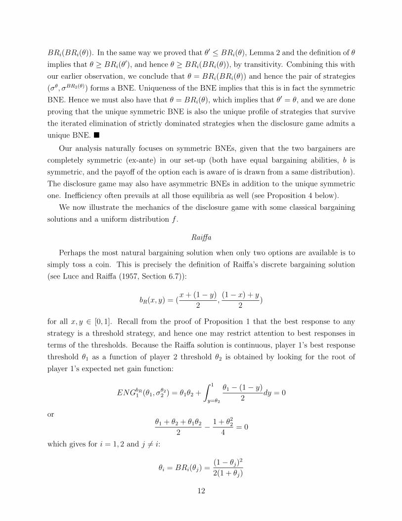
We now illustrate the mechanics of the disclosure game with some classical bargaining

solutions and a uniform distribution f .

Raiffa

Perhaps the most natural bargaining solution when only two options are available is to

simply toss a coin. This is precisely the definition of Raiffa’s discrete bargaining solution

(see Luce and Raiffa (1957, Section 6.7)):

bR(x, y) = (x+ (1− y)

2,(1− x) + y

2)

for all x, y ∈ [0, 1]. Recall from the proof of Proposition 1 that the best response to any

strategy is a threshold strategy, and hence one may restrict attention to best responses in

terms of the thresholds. Because the Raiffa solution is continuous, player 1’s best response

threshold θ1 as a function of player 2 threshold θ2 is obtained by looking for the root of

player 1’s expected net gain function:

ENGbR1 (θ1, σ

θ22 ) = θ1θ2 +

∫ 1

y=θ2

θ1 − (1− y)

2dy = 0

orθ1 + θ2 + θ1θ2

2− 1 + θ2

2

4= 0

which gives for i = 1, 2 and j 6= i:

θi = BRi(θj) =(1− θj)2

2(1 + θj)

12

One can thus conclude that the disclosure game admits a unique BNE, which is the symmetric

equilibrium with common threshold −2 +√

5 ∼ 0.236.

Kalai-Smorodinsky

Consider now Kalai and Smorodinsky’s (1975) bargaining solution. When applied to two

points on the line X, it will pick the lottery so as to equalize the two players’ utility gains

relative to the best feasible option for them (usually called the “utopia point”). Formally:

bKS(x, y) = (max(x, 1− y)

max(x, 1− y) + max(1− x, y),

max(1− x, y)

max(x, 1− y) + max(1− x, y)).

Using the fact that the Kalai-Smorodinsky solution is continuous, equation (1) characterizing

the unique symmetric BNE becomes:

θ2KS +

∫ 1−θKS

y=θKS

[1− y

1− θKS + 1− y− (1− y)]dy +

∫ 1

y=1−θKS

[θKS

θKS + y− (1− y)]dy = 0.

Re-arranging, developing, and making the change of variables z = 1− y in the first part of

the second term yields:

θ2KS −

∫ 1

y=θKS

(1− y)dy +

∫ 1−θKS

z=θKS

z

1− θKS + zdz +

∫ 1

y=1−θKS

θKSθKS + y

dy = 0.

Using integration by parts, this equation reduces to9

3θ2KS − 2θKS + 1

2− (1− θKS)ln(2− 2θKS)− θ2

KSln(1 + θKS) = 0.

Solving this equation numerically yields that θKS is approximately 0.22.

Nash

Consider now Nash’s (1950) bargaining solution. When applied to two points on the

line X this solution picks the lottery that brings the players’ utilities as close as possible to

(1/2, 1/2). Formally:

bN(x, y) =

(max{x, 1− y}, 1−max{x, 1− y}) if max{x, 1− y} ≤ 1

2

(min{x, 1− y}, 1−min{x, 1− y}) if min{12, 1− x} ≥ 1

2

(12, 1

2) otherwise

9Integrating by parts, one gets∫

wα+w = w − αln(α + w), for each α such that α + w > 0. Hence the

sum of the third and fourth terms is equal to [z − (1 − θ)ln(1 − θ + z)]1−θz=θ + θ[y − θln(θ + y)]1y=1−θ, or1− 2θ − (1− θ)ln(2− 2θ) + θ[θ − θln(1 + θ)].

13

As in the previous examples, one may restrict attention to best responses in terms of thresh-

olds, and the Nash solution being continuous, player 1’s best response threshold θ1 as a

function of player 2’s threshold θ2 is obtained by looking for the root of player 1’s expected

net gain function. Following an earlier reasoning, we know that it is a dominant strategy

for both players to reveal their types when above 1/2, and hence one can restrict atttention

to to cases where θ1 and θ2 are no greater than 1/2. The root is thus characterized by the

following equation:

ENGbN1 (θ1, σ

θ22 ) = θ1θ2 +

∫ 1/2

y=θ2

[1

2− (1− y)]dy +

∫ 1−θ1

y=1/2

0dy +

∫ 1

y=1−θ1[θ1 − (1− y)]dy = 0

orθ2

1

2+ θ1θ2 +

θ2

2− θ2

2

2− 1

8= 0

which gives for i = 1, 2 and j 6= i:

θi = BRi(θj) = −θj +

√2θ2

j − θj +1

4

One can thus conclude that the disclosure game admits three BNEs, two in which one player

reveals all his types while the other reveals only when his type is above 1/2, and the unique

symmetric equilibrium where the common threshold equals (−1 +√

3)/4 ∼ 0.183.

4. NORMATIVE ANALYSIS: HOW TO FAVOR DISCLOSURE?

We now introduce a partial ordering on bargaining solutions that will allow us to compare

their performance in terms of efficiency when taking the disclosure game into account. For

any two bargaining solutions b and b′, we will write b′ � b whenever the following condition

holds: (∀x ≤ 1/2)(∀y ≥ x) : b′1(x, y) ≥ b1(x, y) (the symmetry of b and b′ also imply that

(∀y ≤ 1/2)(∀x ≥ y) : b′2(x, y) ≥ b2(x, y)).

Proposition 2 If b′ � b, then the probability of inefficiency in the symmetric equilibrium of

the disclosure game associated with b′ is smaller or equal to the probability of inefficiency in

the symmetric equilibrium of the disclosure game associated with b.

Proof: Recall from the proof of Proposition 1 that the unique symmetric BNE of the

disclosure game associated with any regular bargaining solution involves threshold strategies,

whose common threshold falls in the interior of [0, 12]. Let θ be the threshold associated to b,

and θ′ be the threshold associated to b′. Notice that player 1’s expected net gain of revealing

14

over withholding under b when of type θ′ while the opponent plays the threshold strategy

associated to θ′ is non-positive:

ENGb1(θ′, σθ

′

2 ) ≤ 0. (2)

Indeed, this inequality actually holds pointwise, since b′ � b and player 2 withholds his

information when y < θ′, and is thus preserved through summation.

We are now ready to conclude the proof by showing that θ ≥ θ′ (indeed, the probability

of ending up with an inefficient outcome, i.e. the disagreement point, is equal to the square

of the BNE threshold). Suppose, on the contrary, that θ < θ′, and let θ be a number that

falls between θ and θ′. Remember our first observation in the proof of Proposition 1 that a

player’s expected net gain is increasing in his own type. Inequality (2) thus implies that

ENGb1(θ, σθ

′

2 ) < 0.

Remember also the second observation from the proof of Proposition 1, namely that a player’s

expected net gain does not increase when the opponent reveals more, and hence

ENGb1(θ, σθ2) < 0,

but this contradicts the fact that the threshold strategies associated to θ forms a BNE of

the disclosure game associated to b (as it should be optimal for player 1 to reveal his option

at θ since it is larger than θ). �

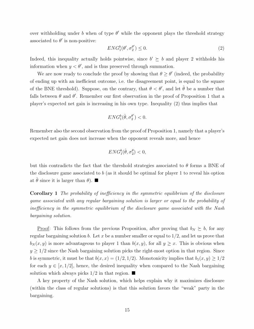
Corollary 1 The probability of inefficiency in the symmetric equilibrium of the disclosure

game associated with any regular bargaining solution is larger or equal to the probability of

inefficiency in the symmetric equilibrium of the disclosure game associated with the Nash

bargaining solution.

Proof: This follows from the previous Proposition, after proving that bN � b, for any

regular bargaining solution b. Let x be a number smaller or equal to 1/2, and let us prove that

bN(x, y) is more advantageous to player 1 than b(x, y), for all y ≥ x. This is obvious when

y ≥ 1/2 since the Nash bargaining solution picks the right-most option in that region. Since

b is symmetric, it must be that b(x, x) = (1/2, 1/2). Monotonicity implies that b1(x, y) ≥ 1/2

for each y ∈ [x, 1/2], hence, the desired inequality when compared to the Nash bargaining

solution which always picks 1/2 in that region. �A key property of the Nash solution, which helps explain why it maximizes disclosure

(within the class of regular solutions) is that this solution favors the “weak” party in the

bargaining.

15

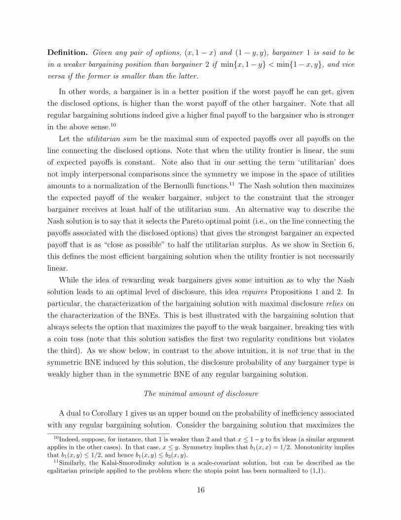
Definition. Given any pair of options, (x, 1 − x) and (1 − y, y), bargainer 1 is said to be

in a weaker bargaining position than bargainer 2 if min{x, 1− y} < min{1− x, y}, and vice

versa if the former is smaller than the latter.

In other words, a bargainer is in a better position if the worst payoff he can get, given

the disclosed options, is higher than the worst payoff of the other bargainer. Note that all

regular bargaining solutions indeed give a higher final payoff to the bargainer who is stronger

in the above sense.10

Let the utilitarian sum be the maximal sum of expected payoffs over all payoffs on the

line connecting the disclosed options. Note that when the utility frontier is linear, the sum

of expected payoffs is constant. Note also that in our setting the term ‘utilitarian’ does

not imply interpersonal comparisons since the symmetry we impose in the space of utilities

amounts to a normalization of the Bernoulli functions.11 The Nash solution then maximizes

the expected payoff of the weaker bargainer, subject to the constraint that the stronger

bargainer receives at least half of the utilitarian sum. An alternative way to describe the

Nash solution is to say that it selects the Pareto optimal point (i.e., on the line connecting the

payoffs associated with the disclosed options) that gives the strongest bargainer an expected

payoff that is as “close as possible” to half the utilitarian surplus. As we show in Section 6,

this defines the most efficient bargaining solution when the utility frontier is not necessarily

linear.

While the idea of rewarding weak bargainers gives some intuition as to why the Nash

solution leads to an optimal level of disclosure, this idea requires Propositions 1 and 2. In

particular, the characterization of the bargaining solution with maximal disclosure relies on

the characterization of the BNEs. This is best illustrated with the bargaining solution that

always selects the option that maximizes the payoff to the weak bargainer, breaking ties with

a coin toss (note that this solution satisfies the first two regularity conditions but violates

the third). As we show below, in contrast to the above intuition, it is not true that in the

symmetric BNE induced by this solution, the disclosure probability of any bargainer type is

weakly higher than in the symmetric BNE of any regular bargaining solution.

The minimal amount of disclosure

A dual to Corollary 1 gives us an upper bound on the probability of inefficiency associated

with any regular bargaining solution. Consider the bargaining solution that maximizes the

10Indeed, suppose, for instance, that 1 is weaker than 2 and that x ≤ 1−y to fix ideas (a similar argumentapplies in the other cases). In that case, x ≤ y. Symmetry implies that b1(x, x) = 1/2. Monotonicity impliesthat b1(x, y) ≤ 1/2, and hence b1(x, y) ≤ b2(x, y).

11Similarly, the Kalai-Smorodinsky solution is a scale-covariant solution, but can be described as theegalitarian principle applied to the problem where the utopia point has been normalized to (1,1).

16

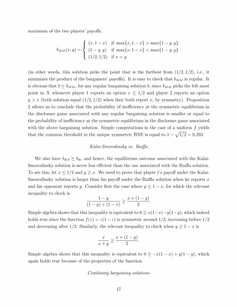
maximum of the two players’ payoffs,

bMM(x, y) =

(x, 1− x) if max{x, 1− x} > max{1− y, y}(1− y, y) if max{x, 1− x} < max{1− y, y}(1/2, 1/2) if x = y

(in other words, this solution picks the point that is the furthest from (1/2, 1/2), i.e., it

minimizes the product of the bargainers’ payoffs). It is easy to check that bMM is regular. It

is obvious that b � bMM , for any regular bargaining solution b, since bMM picks the left-most

point in X whenever player 1 reports an option x ≤ 1/2 and player 2 reports an option

y > x (both solution equal (1/2, 1/2) when they both report x, by symmetry). Proposition

2 allows us to conclude that the probability of inefficiency at the symmetric equilibrium in

the disclosure game associated with any regular bargaining solution is smaller or equal to

the probability of inefficiency at the symmetric equilibrium in the disclosure game associated

with the above bargaining solution. Simple computations in the case of a uniform f yields

that the common threshold in the unique symmetric BNE is equal to 1−√

1/2 ∼ 0.293.

Kalai-Smorodinsky vs. Raiffa

We also have bKS � bR, and hence, the equilibrium outcome associated with the Kalai-

Smorodinsky solution is never less efficient than the one associated with the Raiffa solution.

To see this, let x ≤ 1/2 and y ≥ x. We need to prove that player 1’s payoff under the Kalai-

Smorodinsky solution is larger than his payoff under the Raiffa solution when he reports x

and his opponent reports y. Consider first the case where y ≤ 1− x, for which the relevant

inequality to check is1− y

(1− y) + (1− x)≥ x+ (1− y)

2.

Simple algebra shows that this inequality is equivalent to 0 ≥ x(1−x)−y(1−y), which indeed

holds true since the function f(z) = z(1− z) is symmetric around 1/2, increasing before 1/2

and decreasing after 1/2. Similarly, the relevant inequality to check when y ≥ 1− x is

x

x+ y≥ x+ (1− y)

2.

Simple algebra shows that this inequality is equivalent to 0 ≥ −x(1 − x) + y(1 − y), which

again holds true because of the properties of the function.

Combining bargaining solutions

17

Proposition 2 implies an algorithm that transforms any pair of regular solutions into a

regular solution, which is at least as efficient as each of the two original solutions. A similar

procedure yields a regular solution, which is less efficient than each of the original solutions.

In other words, the partial ordering of solutions according to their efficiency induces a lattice

structure over regular bargaining solutions.

For any pair of regular bargaining solutions, b and b′, let b∨ b′ be the bargaining solution

defined as follows. First,

(b ∨ b′)1(x, y) =

{max{b1(x, y), b′1(x, y)} if min{x, 1− y} ≤ min{1− x, y}min{b1(x, y), b′1(x, y)} if min{x, 1− y} ≥ min{1− x, y}

where (b ∨ b′)2(x, y) = 1 − (b ∨ b′)1(x, y). Second, (b ∨ b′)(x, ∅) = (x, 1 − x) and similarly,

(b ∨ b′)(∅, y) = (1− y, y). In an analogous way we define b ∧ b′, where the only difference is

the following: if bargainer 1 is weak, then (b ∧ b′)1(x, y) equals min{b1(x, y), b′1(x, y)}, and if

bargainer 2 is weak , then (b ∧ b′)1(x, y) equals max{b1(x, y), b′1(x, y)}.

Proposition 3 (i) b ∨ b′ and b ∧ b′ are regular solutions, (ii) b ∨ b′ � b and b ∨ b′ � b′, and

(iii) b � b ∧ b′ and b′ � b ∧ b′.

Proof: To establish (i), first notice that b∨b′ and b∧b′ are well-defined, as min{x, 1−y} =

min{1 − x, y} if and only if x = y, in which case b1(x, y) = b′1(x, y) = 12. Next, it is easy

to check that b ∨ b′ and b ∧ b′ satisfy efficiency and symmetry. Next, consider a pair of

real-valued functions, φ(·) and ϕ(·), defined over some subset of R. If both φ(·) and ϕ(·) are

non-decreasing then so are max{φ(·), ϕ(·)} and min{φ(·), ϕ(·)}. Also, if α is a real number

such that φ(α) = ϕ(α), then h(·), where h(z) = φ(z) if z ≤ α and h(z) = ϕ(z) if z ≥ α, is

also non-decreasing. Hence b∨ b′ and b∧ b′ is monotone (apply these simple facts to x and y

in turn). We conclude by establishing (ii) and (iii). For any x ≤ 1/2 and y ≥ x, we have that

min{x, 1−y} ≤ min{1−x, y}, in which case (b∨ b′)1(x, y) is equal to max{b1(x, y), b′1(x, y)}.By the definition of the partial order �, it follows that b ∨ b′ � b and b ∨ b′ � b′. A similar

argument implies that b � b ∧ b′ and b′ � b ∧ b′. �

Regularity and disclosure

As mentioned above, the regularity conditions may be interpreted as reasonable proper-

ties of a bargaining solution, which is meant to reach a compromise between parties with

conflicting preferences. However, in the simple environment of the previous subsections,

these properties restrict the extent to which bargainers would be willing to disclose options

18

in equilibrium. This is easily seen by noting that a dictatorial bargaining solution guaran-

tees efficiency in our model as it becomes a weakly dominant strategy to always disclose.

Disclosure is also weakly dominant under an (ex-post) inefficient bargaining solution that

implements disagreement unless both bargainers disclose their options.

However, these solutions would not guarantee efficiency in the following two extensions

of our model: (i) introducing an exogenous probability p that a bargainer has no option

to disclose, and (ii) expanding the set of potentially feasible options such that the option

known to one bargainer may be Pareto inferior to the option known to the other bargainer.

While the first extension can be easily accommodated, the second extension is more chal-

lenging. For example, consider the case where each bargainer independently draws a type

from a distribution on [0, 1]2. The difficulty here is that a bargainer’s net expected gain

from disclosing is not necessarily increasing in his type, and hence, proving existence of a

symmetric pure-strategy equilibrium is not straightforward. Furthermore, it is not clear how

such equilibria (if they exist) would look like (i.e., what would be the analogue of the cutoff

strategies of the “one-shot” game).

While monotone bargaining solutions may be appealing to parties in conflict, they restrict

the extent to which bargainers are willing to disclose feasible options. To see why a non-

monotonic solution may out-perform any regular solution, consider the bargainer solution

that selects the disclosed option, which maximizes the payoff for the weak bargainer. Note

this is a “deterministic” variant of the Nash solution, which always picks the option that max-

imizes the product of the players’ payoffs without ever trying to compromise through the use

of lotteries (unless there is a tie, in which case a coin toss determines which option is chosen).

This solution violates the monotonicity condition that is part of the definition of a regular

solution. Indeed, it picks (1/2, 1/2) if the set of available options is {(1/3, 2/3), (1/2, 1/2)},and (1/3, 2/3) if the set of available options is {(1/3, 2/3), (3/4, 1/4)}. Player 1’s payoff

thereby decreases, while the available options become more favorable to him. When f is

uniform, the one-shot disclosure game induced by this solution has a symmetric BNE where

the probability of disclosure in equilibrium is given by

σ(x) =

{−1

3+ 4

3( 1

2−4x)32 if x ≤ 1

4

1 if x > 14

The aggregate probability with which a bargainer withholds his information is equal to 0.138,

and hence, the overall probability of inefficiency is lower than under any regular bargaining

solution.

Note that the equilibrium threshold induced by the above bargaining solution is actually

higher than the threshold induced by the monotonic Nash solution. The reason the non-

19

monotonic solution is more efficient stems from the fact that every type discloses with some

positive probability. This highlights the difficulty in characterizing the most efficient bar-

gaining solution among those that are symmetric and ex-post efficient, but not necessarily

monotone. Providing such a characterization remains an open problem.

Asymmetric BNEs

As explained earlier, it is natural to focus on symmetric BNEs given the symmetry in

the model. Yet one may wonder what happens when one considers asymmetric BNEs as

well. When f is symmetric (i.e. f(x) = f(1 − x), for all x ∈ [0, 1]), the Nash solution is

still the best among all continuous regular solutions, in that it is the only one for which

the disclosure game admits an efficient BNE. While identifying the best solution for general

densities remains an open question, we also observe that efficiency is out of reach in the

disclosure game at any BNE and for any continuous regular bargaining solutions (including

Nash) whenever it is more likely to discover options that are relatively more favorable in the

sense that f(x) > f(1− x), for all x ≥ 1/2.

Proposition 4 Let b be a regular bargaining solution that is continuous. If f is symmetric,

then efficiency in the disclosure game associated to b is obtained at some BNE only if b is

the Nash solution. If it is more likely to discover options that are relatively more favorable

in the sense that f(x) > f(1− x), for all x ≥ 1/2, then the outcome associated to any BNE

of the disclosure game associated to b is inefficient.

Proof: We showed in the proof of the previous proposition that any BNE must involve

threshold strategies. Hence, for a BNE to be efficient, it must be that at least one of the two

bargainers follows a fully revealing strategy. To fix ideas, suppose that we have a BNE in

which the second bargainer systematically reveals the option he is aware of. Note that the

first bargainer’s expected net gain from disclosing when of type 12

is given by∫ 1

y=0

[b1(1

2, y)− (1− y)]f(y)dy.

This expression can be decomposed into two components: one where the opponent’s type is

below 12, and another where his type is above 1

2. The second component may be rewritten

as follows. First, using the symmetry of b we replace b1(12, y) by b2(y, 1

2). Second, b2(y, 1

2) =

1−b1(y, 12). Third, by symmetry of b, we have that b1(y, 1

2) = b1(1

2, 1−y). Making the change

of variable y′ ≡ 1− y , it follows that the net expected gain of type 12

equals

∫ 12

y=0

[b1(1

2, y)− (1− y)]f(y)dy +

∫ 12

y′=0

[1− b1(1

2, y′)− y′)]f(1− y′)dy. (3)

20

If f is symmetric, then this expression is equal to zero, and hence the first bargainer’s

best response to the fully revealing strategy is to reveal if and only if his type is larger or

equal to 1/2. Let’s check now that systematic revelation is a best response for the second

bargainer. Notice that ∫ 1

x=1/2

(b2(x, 0)− (1− x))f(x)dx

cannot be strictly negative, as the second bargainer’s expected net gain of disclosing would

then be negative when his type is very small. Given that b2(x, 0) ≤ 1− x, for all x ∈ [1/2, 1]

and that b2 is continuous, it must thus be that b2(x, 0) = 1−x, for all x ∈ [1/2, 1]. The third

regularity condition implies that b2(x, y) = 1−x, for all y ≤ 1/2 and all x ∈ [1/2, 1−y]. The

second regularity condition then implies that b2(x, y) = max{1−x, y} if max{1−x, y} ≤ 1/2

and = min{1−x, y} if min{1−x, y} ≥ 1/2. Similar conditions apply for the first bargainer’s

payoffs, by symmetry. Consider now a case where both x and y are no larger than 1/2.

The third regularity condition implies that the first bargainer’s payoff is no larger than

b1(1/2, y) = 1/2 and the second bargainer’s payoff is no larger than b2(x, 1/2) = 1/2. Hence

b(x, y) = (1/2, 1/2). Symmetry implies that a similar argument applies when both x and y

are no smaller than 1/2. Hence b must coincide with the Nash solution. When b is the Nash

solution, the second bargainer is indifferent between revealing or not when of type y = 0

given that the opponent systematically reveals. Hence full disclosure is a best response and

we have identified an efficient BNE.

Suppose now that f(x) > f(1−x), for all x ≥ 1/2. In that case, expression (3) Is strictly

positive, and hence the threshold for the first bargainer’s best reponse strategy is strictly

smaller than 1/2. Let’s call it θ. Then the second bargainer’s expected net gain of revealing

when of type y = 0 is equal to∫ 1

x=θ

(b2(x, 0)− (1− x))f(x)dx.

As before, observe that∫ 1

x=θ(b2(x, 0)−(1−x))f(x)dx ≤ 0. On the other hand, it must also be

that∫ 1/2

x=θ(b2(x, 0)− (1−x))f(x)dx < 0 for any regular b, as b2(x, 0) ≤ b2(0, 0) = 1/2 < 1−x,

for all 0 < x < 1/2. Hence systematic revelation cannot be a best response when the other

bargainer use a threshold strategy that discloses some types below 1/2, and there is no way

to achieve efficiency in any BNE of the disclosure game. �

Knowing Multiple Options

Consider now a case where each bargainer knows about the feasibility of k options on the

line. Formally, i’s type is a subset Oi of [0, 1] (determining i’s own payoff - same convention

21

as the one described at the beginning of Section 2) that contains k elements obtained from

repeated independent draws that follow the density f . Suppose that the first bargainer has

disclosed a subset X1 of O1, while the second bargainer has disclosed a subset X2 of O2.

The feasible set in the space of utilities in that case is the smallest triangle that contains all

the following vectors: (0, 0), (x1, 1 − x1), for all x1 ∈ X1, and (1 − x2, x2), for all x2 ∈ X2.

Equivalently, if (x, 1− x) is the most advantageous vector in that list for the first bargainer

and (1− y, y) is the most advantageous in that list for the second bargainer, then the feasible

set in the space of utilities is the triangle with extreme points (0, 0), (x, 1− x) and (1− y, y).

A bargaining solution is welfarist if it solves bargaining problems by paying attention only

to feasible sets of utilities and the disagreement point. Bargaining solution defined in Nash’s

(1950) bargaining model is welfarist, and so are in particular his solution, the Raiffa solution,

and the Kalai-Smorodinsky solution. An example of solution that is not welfarist is one that

would pick the middle option when three have been disclosed. Suppose we focus on welfarist

solutions. Notice that the regularity conditions thus also have implications in situations

where more than two options have been disclosed, given that any such problem can be

brought down to a problem where only two options have been disclosed, as just shown.

Consider now the extended disclosure game where a pure strategy for either bargainer is

any subset of his type. For each subset Xi of [0, 1], let m(Xi) denote its maximal element.

It is then not difficult to show the following. 1) If a pair of mixed strategies (ρ1, ρ2) forms

a BNE in the extended disclosure game for a given regular bargaining solution, then ρi(Oi)

places positive weight on a nonempty subset Xi of Oi only if m(Xi) = m(Oi). In addition,

the total probability placed on those sets according to ρi(Oi) (i.e. versus the probability

placed on reporting the empty set) varies only with m(Oi). Finally, the pair of strategies

(σ1, σ2), where the probability σi(x) of revealing an option x is equal to the common total

probability of revealing some non-empty subset according to ρi at any type Oi such that

m(Oi) = x, forms a BNE in our original disclosure game for the same bargaining solution

with a density fk. 2) Conversely, if a pair of strategies (σ1, σ2) forms a BNE of the disclosure

game for a given regular bargaining solution and a density fk, then the pair of strategies

(ρ1, ρ2), where ρi amounts to disclose {m(Oi)} with probability σi(m(Oi)) and to disclose

the empty set with the complementary probability, forms a BNE of the extended disclosure

game for that same bargaining solution and with density f for each independent draw that

determines the content of Oi. Given this isomorphism between the BNEs of the extended

disclosure game, and the BNEs of the original bargaining game with density fk, we see that

all the results established so far admit a direct analogue in the case where parties know

multiple options.

22

5. DISCLOSURE OVER TIME

One may argue that players would not remain silent if the outcome of the static game

is inefficient because none of them spoke up. It is thus important to discuss the dynamic

extension of our game. The bargainers now decide when to speak, and the solution is

implemented as soon as at least one option has been disclosed. For simplicity, we will restrict

attention right away to symmetric pure-strategy Bayesian Nash equilibria. A strategy is a

measurable function τ : [0, 1]→ R+∪{∞}, which determines for each type x the time τ(x) at

which to reveal x.12 Measurability means that the inverse image of any Lebesgue measurable

set (in particular any interval) is Lebesgue measurable: τ−1(T ) = {x ∈ [0, 1]|τ(x) ∈ T} is

Lebesgue measurable if T is Lebesgue measurable. It guarantees that a player’s expected

utility when his opponent is known to reveal over some given interval of time, is well-defined.

Utilities are discounted exponentially over time following a discount factor δ < 1. The

outcome when player 1 is of type x, while player 2 is of type y, and they both implement the

strategy τ , is x at time τ(x) if τ(x) < τ(y), y at time τ(y) if τ(x) > τ(y), and b(x, y) at time

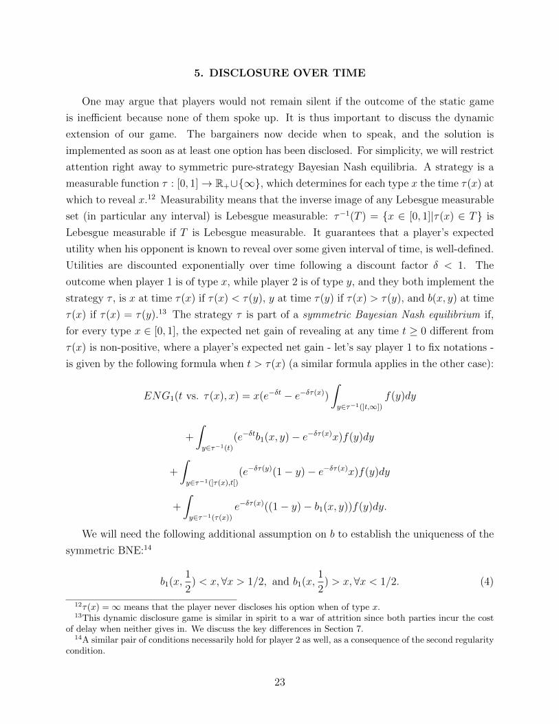
τ(x) if τ(x) = τ(y).13 The strategy τ is part of a symmetric Bayesian Nash equilibrium if,

for every type x ∈ [0, 1], the expected net gain of revealing at any time t ≥ 0 different from

τ(x) is non-positive, where a player’s expected net gain - let’s say player 1 to fix notations -

is given by the following formula when t > τ(x) (a similar formula applies in the other case):

ENG1(t vs. τ(x), x) = x(e−δt − e−δτ(x))

∫y∈τ−1(]t,∞])

f(y)dy

+

∫y∈τ−1(t)

(e−δtb1(x, y)− e−δτ(x)x)f(y)dy

+

∫y∈τ−1(]τ(x),t[)

(e−δτ(y)(1− y)− e−δτ(x)x)f(y)dy

+

∫y∈τ−1(τ(x))

e−δτ(x)((1− y)− b1(x, y))f(y)dy.

We will need the following additional assumption on b to establish the uniqueness of the

symmetric BNE:14

b1(x,1

2) < x,∀x > 1/2, and b1(x,

1

2) > x,∀x < 1/2. (4)

12τ(x) =∞ means that the player never discloses his option when of type x.13This dynamic disclosure game is similar in spirit to a war of attrition since both parties incur the cost

of delay when neither gives in. We discuss the key differences in Section 7.14A similar pair of conditions necessarily hold for player 2 as well, as a consequence of the second regularity

condition.

23

The weak inequality is implied by the first regularity condition. Requiring a strict inequal-

ity is a mild additional requirement which is satisfied by all the classical solutions (Kalai-

Smorodinsky, Nash and Raiffa). Notice, on the other hand, that the max-max solution

(bMM) does not satisfy this additional condition.

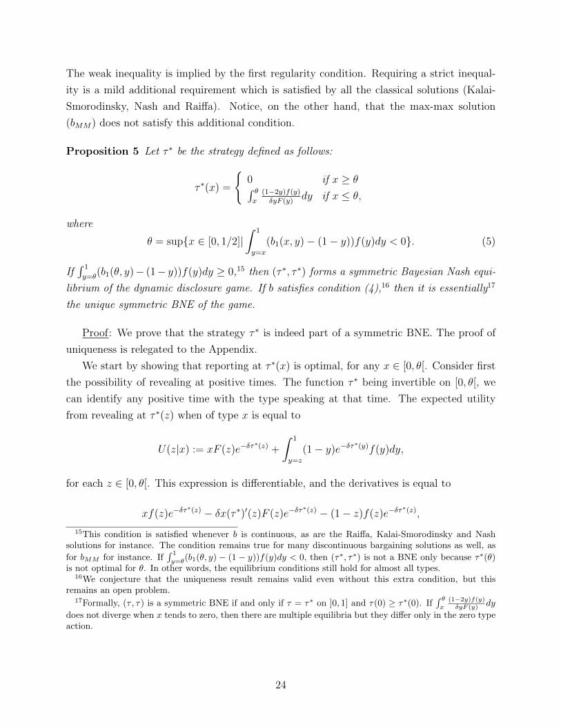
Proposition 5 Let τ ∗ be the strategy defined as follows:

τ ∗(x) =

{0 if x ≥ θ∫ θx

(1−2y)f(y)δyF (y)

dy if x ≤ θ,

where

θ = sup{x ∈ [0, 1/2]|∫ 1

y=x

(b1(x, y)− (1− y))f(y)dy < 0}. (5)

If∫ 1

y=θ(b1(θ, y)− (1− y))f(y)dy ≥ 0,15 then (τ ∗, τ ∗) forms a symmetric Bayesian Nash equi-

librium of the dynamic disclosure game. If b satisfies condition (4),16 then it is essentially17

the unique symmetric BNE of the game.

Proof: We prove that the strategy τ ∗ is indeed part of a symmetric BNE. The proof of

uniqueness is relegated to the Appendix.

We start by showing that reporting at τ ∗(x) is optimal, for any x ∈ [0, θ[. Consider first

the possibility of revealing at positive times. The function τ ∗ being invertible on [0, θ[, we

can identify any positive time with the type speaking at that time. The expected utility

from revealing at τ ∗(z) when of type x is equal to

U(z|x) := xF (z)e−δτ∗(z) +

∫ 1

y=z

(1− y)e−δτ∗(y)f(y)dy,

for each z ∈ [0, θ[. This expression is differentiable, and the derivatives is equal to

xf(z)e−δτ∗(z) − δx(τ ∗)′(z)F (z)e−δτ

∗(z) − (1− z)f(z)e−δτ∗(z),

15This condition is satisfied whenever b is continuous, as are the Raiffa, Kalai-Smorodinsky and Nashsolutions for instance. The condition remains true for many discontinuous bargaining solutions as well, as

for bMM for instance. If∫ 1

y=θ(b1(θ, y) − (1 − y))f(y)dy < 0, then (τ∗, τ∗) is not a BNE only because τ∗(θ)

is not optimal for θ. In other words, the equilibrium conditions still hold for almost all types.16We conjecture that the uniqueness result remains valid even without this extra condition, but this

remains an open problem.17Formally, (τ , τ) is a symmetric BNE if and only if τ = τ∗ on ]0, 1] and τ(0) ≥ τ∗(0). If

∫ θx

(1−2y)f(y)δyF (y) dy

does not diverge when x tends to zero, then there are multiple equilibria but they differ only in the zero typeaction.

24

or(1− z)

zf(z)(x− z)e−δτ

∗(z)

after rearranging the terms and using the definition of τ ∗ to compute (τ ∗)′. We see that the

first order condition is satisfied at z = x, and that the derivative is positive when z < x and

negative when x < z. Hence there is no profitable deviation to a positive time different from

τ ∗(x), when of type x. Deviating to report at zero is not profitable either, as the expected

payoff in that case is

xF (θ) +

∫ 1

y=θ

b1(x, y)f(y)dy

which is equal to

U(θ|x) +

∫ 1

y=θ

(b1(x, y)− (1− y))f(y)dy.

For any ε > 0 small enough, using the third regularity condition, this expression is lower or

equal to

U(θ|x) +

∫ 1

y=θ−ε(b1(θ − ε, y)− (1− y))f(y)dy +

∫ θ

y=θ−ε((1− y)− b1(θ − ε, y))f(y)dy.

The second term is negative, for all ε > 0, by definition of θ. Hence, taking the limit when

ε decreases to zero, we get that the expected utility of reporting at zero is no greater than

U(θ|x), which in turn, by our previous reasoning, is smaller than the expected utility of

reporting at τ(x). This establishes the optimality of τ ∗, for any type strictly in between 0

and θ.

Consider now a type x ∈]θ, 1]. The expected utility of revealing at a time t is equal to

U(z|x), where z is the unique real number in [0, θ[ such that τ ∗(z) = t. Our earlier reasoning

regarding U ’s derivative implies that this expected utility is strictly lower than U(θ|x) (since

z < θ ≤ x), which is equal to xF (θ) +∫ 1

y=θ(1 − y)f(y)dy. Notice that

∫ θ+εy=θ

(b1(x, y) − (1 −y))f(y)dy converges to zero as ε decreases to zero. Hence U(z|x) < U(θ|x) +

∫ θ+εy=θ

(b1(x, y)−(1− y))f(y)dy, for any ε > 0 that is small enough. This in turn implies that

U(z|x) < U(θ|x) +

∫ θ+ε

y=θ

(b1(x, y)− (1− y))f(y)dy +

∫ 1

y=θ+ε

(b1(θ + ε, y)− (1− y))f(y)dy,

by definition of θ. Applying now the third regularity condition (ε is small enough so that

x > θ + ε), we conclude that

U(z|x) < U(θ|x) +

∫ θ+ε

y=θ

(b1(x, y)− (1− y))f(y)dy +

∫ 1

y=θ+ε

(b1(x, y)− (1− y))f(y)dy.

25

Notice that the right-hand side is the expected utility for type x of revealing at zero, and we

have thus proved the optimality of τ ∗ for any type no smaller than θ.

Finally, if x = θ, then a similar reasoning as in the last paragraph implies that revealing

at a positive time leads to a payoff that is no larger than U(θ|θ) = θF (θ)+∫ 1

y=θ(1−y)f(y)dy.

Revealing at zero leads to the expected payoff θF (θ) +∫ 1

y=θb1(x, y)f(y)dy. The condition∫ 1

y=θ(b1(θ, y)− (1− y))f(y)dy ≥ 0 thus guarantees that revealing at zero is optimal for type

θ, as desired. �

The equilibrium behavior in the dynamic game is a natural variant of the equilibrium

behavior in the static game studied previously. Indeed, there is a threshold above which

players reveal their options, while lower types now reveal with delay instead of withholding

their information forever due to the rules of the game. It turns out that the partial ordering

identified in Proposition 2 continues to predict the efficiency of disclosure in the dynamic

game as well.

Proposition 6 Let b and b′ be two regular bargaining solutions that satisfy (4), and let τ

and τ ′ be the strategies in the symmetric BNE of the dynamic disclosure game associated to

b and b′ respectively. If b′ � b, then τ ′(x) ≤ τ(x), for each x ∈ [0, 1].

Proof: Given the characterization of the symmetric BNE in Proposition 5, we see that

proving τ ′(x) ≤ τ(x), for each x ∈ [0, 1], is equivalent to proving θ′ ≤ θ, where θ and θ′ are

the thresholds defined in (5) for b and b′ respectively. Suppose, to the contrary of what we

want to prove, that θ′ > θ. Then for any ε > 0 small enough so that θ′ − ε > θ, we have:∫ 1

y=θ′−ε(b1(θ′ − ε, y)− (1− y))f(y)dy ≥ 0,

by definition of θ. Since b′ � b, we must also have∫ 1

y=θ′−ε(b′1(θ′ − ε, y)− (1− y))f(y)dy ≥ 0,

but this contradicts the definition of θ′. Hence θ′ ≤ θ, as desired. �Hence, disclosure is faster with Nash, than with Kalai-Smorodinsky, than with Raiffa,

and any pair of regular solutions can be combined as in the previous Section to derive a

solution where disclosure is faster, and another where disclosure is slower.

Dynamic vs. static

In comparing between the dynamic and the static versions of the disclosure game, we

begin by showing that for any regular bargaining solution satisfying condition (4), the lowest

26

type to disclose in the static game is lower than the lowest type who discloses immediately

in the dynamic game.

Proposition 7 Let b be a regular bargaining solution that satisfies (4). Let θS and θD be

the thresholds given by (1) and (5), respectively (i.e., the former is the cutoff of the one-shot

simulatenous game, while the latter is the cutoff of the dynamic game). Then θS ≤ θD.

Proof: Assume θS > θD and let θ be a player type between θS and θD. Consider the static

disclosure game first. Assume player j uses the symmetric equilibrium strategy associated

with the threshold θS. Then for type x of player i, the expected net gain from disclosing,

given by

xF (θS) +

∫ 1

θS

[bi(x, y)− (1− y)]f(y)dy

is positive for all x > θS and negative for all x < θS. In particular, it is negative for

x = θ < θS. Since θF (θS) is strictly positive, it follows that∫ 1

θS

[bi(θ, y)− (1− y)]f(y)dy < 0

Because θS ≤ 12, we have that 1− y > θ for all θ ≤ y ≤ θS. Hence, bi(θ, y) ≤ (1− y) for all

θ ≤ y ≤ θS. Therefore, ∫ 1

θ

[bi(θ, y)− (1− y)]f(y)dy < 0

This contradicts the definition of θD < θ in Proposition 7. �

Example 1. To illustrate Proposition 7, we compute the equilibrium threshold of the dy-

namic game associated with the Raiffa ( θRD), Kalai-Smorodinsky ( θKSD ) and Nash solutions

( θND) for a uniform distribution. By the continuity of these bargaining solutions, the three

thresholds are given by the solutions between 0 and 12

to the following equations:

∫ 1

y=θRD

θRD − (1− y)

2dy = 0

which yields θRD = 13

(compared with θRS = 0.24 in the static game),

∫ 1−θKSD

y=θKSD

[1− y

1− θKSD + 1− y− (1− y)]dy +

∫ 1

y=1−θKSD

[θKSD

θKSD + y− (1− y)]dy = 0

27

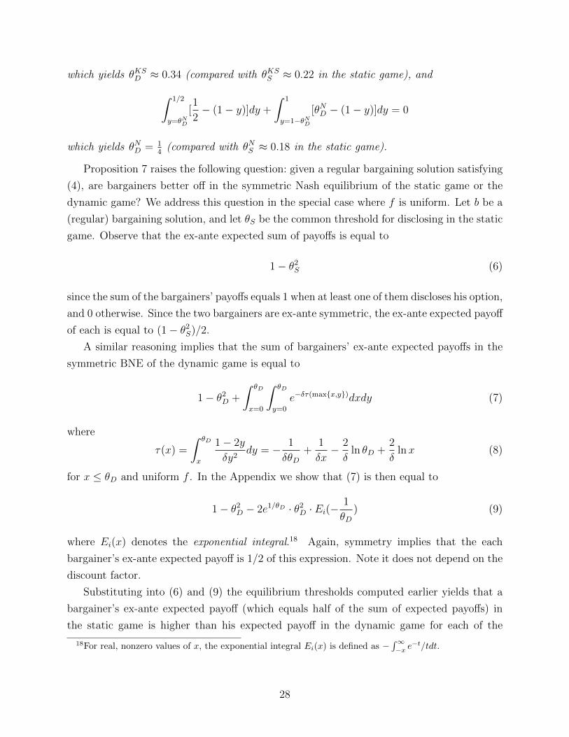
which yields θKSD ≈ 0.34 (compared with θKSS ≈ 0.22 in the static game), and∫ 1/2

y=θND

[1

2− (1− y)]dy +

∫ 1

y=1−θND[θND − (1− y)]dy = 0

which yields θND = 14

(compared with θNS ≈ 0.18 in the static game).

Proposition 7 raises the following question: given a regular bargaining solution satisfying

(4), are bargainers better off in the symmetric Nash equilibrium of the static game or the

dynamic game? We address this question in the special case where f is uniform. Let b be a

(regular) bargaining solution, and let θS be the common threshold for disclosing in the static

game. Observe that the ex-ante expected sum of payoffs is equal to

1− θ2S (6)

since the sum of the bargainers’ payoffs equals 1 when at least one of them discloses his option,

and 0 otherwise. Since the two bargainers are ex-ante symmetric, the ex-ante expected payoff

of each is equal to (1− θ2S)/2.

A similar reasoning implies that the sum of bargainers’ ex-ante expected payoffs in the

symmetric BNE of the dynamic game is equal to

1− θ2D +

∫ θD

x=0

∫ θD

y=0

e−δτ(max{x,y})dxdy (7)

where

τ(x) =

∫ θD

x

1− 2y

δy2dy = − 1

δθD+

1

δx− 2

δln θD +

2

δlnx (8)

for x ≤ θD and uniform f . In the Appendix we show that (7) is then equal to

1− θ2D − 2e1/θD · θ2

D · Ei(−1

θD) (9)

where Ei(x) denotes the exponential integral.18 Again, symmetry implies that the each

bargainer’s ex-ante expected payoff is 1/2 of this expression. Note it does not depend on the

discount factor.

Substituting into (6) and (9) the equilibrium thresholds computed earlier yields that a

bargainer’s ex-ante expected payoff (which equals half of the sum of expected payoffs) in

the static game is higher than his expected payoff in the dynamic game for each of the

18For real, nonzero values of x, the exponential integral Ei(x) is defined as −∫∞−x e

−t/tdt.

28

three bargaining solutions. Specifically, the ex-ante expected payoff for the Raiffa solution is

0.472 in the dynamic game and 0.474 in the static game; for Kalai-Smorodinsky, the ex-ante

expected payoff is 0.473 in the dynamic game and 0.476 in the static game; and finally, for

the Nash solution, the ex-ante expected payoffs in the dynamic and static games are 0.481

and 0.483, respectively. Though the magnitudes are not large, the quantitative result is

interesting. Without thinking much about the problem, one could think that the dynamic

procedure should perform better than the static one because bargainers have an opportunity

to speak if nobody has spoken right away. Of course this need not be so because changing the

procedure changes the bargainers’ incentives to disclose their option, and will in fact make

them less likely to disclose right away, as shown in Proposition 7. These computations for a

uniform distribution illustrates that this negative effect may overcome the positive effect of

letting the bargainers more time to speak. It remains an open question whether this is true

for all regular bargaining solutions and for all symmetric distributions.

Dynamic disclosure with an opportunity to react

As a natural variant of our dynamic game, we study a situation where bargainers have

one last chance to disclose their option right after the other has proken, i.e. right before b

is implemented. Note that the strategies in this game are richer than those of the original

dynamic game. As in the original game, they specify the latest period in which a bargainer

would disclose if the other party has not done so. But in addition, for every history which

ended with disclosure by the other party, a bargainer’s strategy also specifies whether or

not he would disclose as a function of the other party’s disclosed type and the period of

disclosure. To eliminate notational complications and unlikely off-equilibrium behavior, we

focus on a slightly refined notion of BNE. Indeed, we will assume that type x discloses right

after the other party has disclosed a type y if and only if y > 1−x. In other words, we focus

on equilibria in which a bargainer discloses immediately after the other party has disclosed

whenever it is optimal for him to do so (whenever the the payoff from the other party’s

option is lower than the payoff from his own option). Given this restriction, strategies in a

refined BNE are measurable functions τ : [0, 1] → R+ ∪ {∞}, that describe when a player

discloses his option as a function of his type.

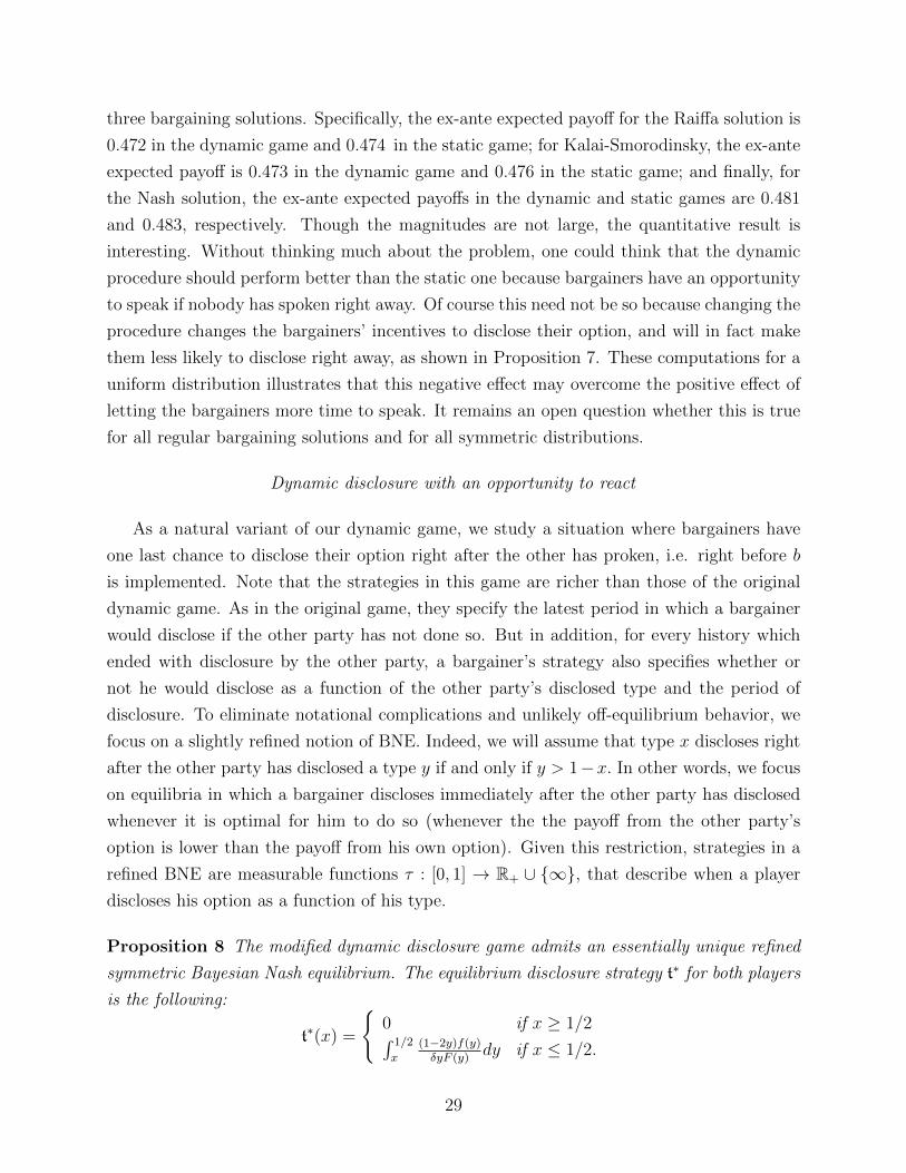
Proposition 8 The modified dynamic disclosure game admits an essentially unique refined

symmetric Bayesian Nash equilibrium. The equilibrium disclosure strategy t∗ for both players

is the following:

t∗(x) =

{0 if x ≥ 1/2∫ 1/2

x(1−2y)f(y)δyF (y)

dy if x ≤ 1/2.

29

Proof: We prove that the strategy t∗ is indeed part of a symmetric BNE. The proof of

uniqueness is relegated to the Appendix.

We start by showing that reporting at t∗(x) is optimal, for any x ∈ [0, 1/2[. Consider

first the possibility of revealing at positive times. The function t∗ being invertible on [0, 1/2[,

we can identify any positive time with the type speaking at that time. The expected utility

from revealing at t∗(z) when of type x is equal to

U(z|x) := xF (z)e−δt∗(z) +

∫ 1−x

y=z

(1− y)e−δt∗(y)f(y)dy +

∫ 1

y=1−xb1(x, y)e−δt

∗(y)f(y)dy,

for each z ∈ [0, 1/2[. It is easy to check that this expression is differentiable, and has the

same derivative as the similar expression in the proof of Proposition 5 (because the third

term does not depend on z), i.e.

(1− z)

zf(z)(x− z)e−δt

∗(z).

We see that the first order condition is satisfied at z = x, and that the derivative is positive

when z < x and negative when x < z. Hence there is no profitable deviation to a positive

time different from t∗(x), when of type x. Deviating to report at zero is not profitable either,

as the expected payoff in that case is

x

2+

∫ 1

y=1/2

b1(x, y)f(y)dy

which is equal to

U(1/2|x) +

∫ 1−x

y=1/2

(b1(x, y)− (1− y))f(y)dy,

and the second term of this expression is non-positive, as y ≤ 1− x implies that x ≤ 1− yand hence b1(x, y) ≤ 1− y.

Consider now a type x ∈ [1/2, 1]. The expected utility of revealing at a positive time t,

corresponding to a z < 1/2, is equal to

xF (z)e−δt∗(z) +

∫ 1−x

y=z

(1− y)e−δt∗(y)f(y)dy +

∫ 1

y=1−xb1(x, y)e−δt

∗(y)f(y)dy,

if z ≤ 1− x, and to

xF (z)e−δt∗(z) +

∫ 1

y=z

b1(x, y)e−δt∗(y)f(y)dy,

if z ≥ 1 − x. The expression when z ≤ 1 − x is non-decreasing in z, as was U(z|x) when

30

x was smaller than 1/2. The expression when z ≥ 1 − x is also non-decreasing because its

derivative is equal to

(1− zz

x− b1(x, z))f(z)e−δt∗(z).

Notice that z ≥ 1− x implies x ≥ 1− z and hence b1(x, z) ≤ x. On the other hand, z ≤ 1/2

implies that (1 − z)/z ≥ 1, and hence b1(x, z) ≤ (x(1 − z))/z, which implies that the last

derivative in non-negative, as desired. The expected utility of revealing at a positive t is

thus no larger than when taking the limit of that expected utility when z tends to 1/2, i.e.x2

+∫ 1

y=1/2b1(x, y)f(y)dy. But this is exactly the expected utility the player gets by revealing

at zero, which shows that there are no profitable deviations when x ∈ [1/2, 1] either. �

By Proposition 8, the timing of disclosure in the unique refined symmetric BNE is inde-

pendent of the bargaining solution. Furthermore, independently of the bargaining solution,

every type above 12

delays the latest time at which he would disclose, relative to his timing of

disclosure in the original dynamic game (where a bargainer cannot disclose immediately after

his rival). Hence, for every bargaining solution, the ex-ante expected payoff of a bargainer is

lower in this dynamic game than in the original game discussed above. Again, one sees that

more opportunities to speak can in fact be damaging in terms of welfare.

6. MORE GENERAL UTILITY FRONTIERS

In this section we investigate how our analysis of the static disclosure game would change,

if the utility frontier X was not linear. We first note that all of our general results (i.e., those

that did not involve the specific bargaining solutions of Raiffa, Kalai-Smorodinsky and Nash)

in Sections 3 and 4 continue to hold for any bounded utility frontier u2 = g(u1), which is

symmetric (if X contains a point where bargainer 1 gets x and bargainer 2 gets y, then

X also contains the point where 1 gets y and 2 gets x) and has no Pareto comparisons (to

adapt the results to the more general environment, one needs to replace 1− y with g−1(y)).

Extending the utility frontier beyond a line with slope −1 has several implications. First,

while the Raiffa solution is monotone independently of the shape of X, the Nash and Kalai-

Smorodinsky solutions need not be.19 Second, the Nash, Kalai-Smorodinsky and Raiffa

solutions may no longer be comparable according to the partial ordering characterized in

Proposition 2.20 Finally, as we show below, the Nash bargaining solution is no longer the

most efficient.19To see this in the case of the Nash solution, for instance, consider some concave frontier g and let

u∗ = g(u∗). Take a pair of symmetric options (x, g(x)) and (g(x), x), where x < u∗ < g(x). The Nashsolution gives each bargainer an expected payoff of 1

2 [x+g(x)], which is strictly lower than u∗. Next considerthe pair of options (u∗, u∗) and (g(x), x). The Nash solution associated with these options is (u∗, u∗), andhence, bargainer 2’s expected payoff went up, even though (u∗, u∗) is worse for him than (x, g(x)).

20For example, consider the following convex utility frontier: g(u1) = 1 − 2u1, if u1 ≤ 13 , and g(u1) =

31

u1

u2

X, or u2=g(u1)

45-degree line

u*

u*

x

y

g(x)

x+g(x)(utilitarian surplus)

(x+g(x))/2

b*(x,y)

Figure 1

is no longer the most efficient.Characterizing the most efficient regular bargaining solution for any symmetric and

decreasing g remains an open question. However, Proposition 4 implies an algorithmthat transforms any pair of regular solutions into a regular solution, which is at least asefficient as each of the two original solutions. By imposing additional structure on g, weare able to say more than this. In particular, if we assume that g is differentiable andis either convex or concave, then we are able to characterize the most efficient regularbargaining solution.

Consider first the case in which g is differentiable and convex. Our first observationis the set of regular bargaining solution still contains the well-known bargaining solutionsthat we discussed.

Proposition 9 The Raiffa, Nash and Kalai-Smorodinsky solutions are all regular on X.

Proof: See the Appendix. �Let b∗ be the bargaining solution defined as follows (see the discussion following

Corollary 1). If two options were disclosed, it selects the lottery over these two options,which maximizes the expected payoff to the weak bargainer, subject to the constraintthat the expected payoff to the strong bargainer is at least half the utilitarian surplus(see Figure 1). If only one option was disclosed, it selects that option with certainty.Observe that b∗ describes the Nash solution when g is linear.

Lemma 3 b∗ is a regular bargaining solution.

Proof: See the Appendix. �

25

Characterizing the most efficient regular bargaining solution for any symmetric and de-

creasing g remains an open question. However, Proposition 3 implies an algorithm that

transforms any pair of regular solutions into a regular solution, which is at least as efficient

as each of the two original solutions. By imposing additional structure on g, we are able to

say more than this. In particular, if we assume that g is differentiable and is either convex

or concave, then we are able to characterize the most efficient regular bargaining solution.

Consider first the case in which g is differentiable and convex. Note that this curve

describes the support of the payoffs associated with the potentially feasible options - it is

not the Pareto frontier of the set of feasible agreements as in a standard bargaining problem

(in our model the set of feasible agreements consists of two points randomly drawn from

the curve). Note also that the case of a convex curve is interesting not merely for the sake

of generalization. It allows to capture situations where a bargainer would not disclose an

option, which is only slightly worse for him but much better for the other bargainer (e.g., the

first bargainer may disclose (1, 1) but not (0, 100)). Our first observation is the set of regular

bargaining solution still contains the well-known bargaining solutions that we discussed.

Proposition 9 The Raiffa, Nash and Kalai-Smorodinsky solutions are all regular on X.

Proof: See the Appendix. �

Let b∗ be the bargaining solution defined as follows (see the discussion following Corollary

1). If two options were disclosed, it selects the lottery over these two options, which maxi-

mizes the expected payoff to the weak bargainer, subject to the constraint that the expected

12−

12u1, otherwise. For the pair ( 1

4 ,12 ) and ( 5

12 ,724 ) it easy to show that the Kalai-Smorodinsky solution gives

a higher expected payoff to bargainer 1 than the Nash solution, which in turn gives a higher expected payoffthan the Raiffa solution. However, for the pair ( 1

4 ,12 ) and ( 7

24 ,512 ), the Raiffa solution gives bargainer 1 a

higher expected payoff than the Kalai-Smorodinsky solution, which in turn, gives a higher expected payoffthan the Nash solution.

32

payoff to the strong bargainer is at least half the utilitarian surplus (see Figure 1). If only

one option was disclosed, it selects that option with certainty. Observe that b∗ describes the

Nash solution when g is linear.

Lemma 3 b∗ is a regular bargaining solution.

Proof: See the Appendix. �

We now prove that b∗ is the most efficient (in the sense of minimizing the probability

that no option is disclosed) regular bargaining solution when g is differentiable and convex.

To understand the intuition for this result, note that in order to motivate bargainers to

disclose, the solution needs to favor the weakest bargainer (this follows from Proposition

2). However, if the solution is too biased in favor of the weakest bargainer, it may violate

monotonicity. For example, suppose g(x) > x, g−1(y) > y, and y > x (as in Figure 1 again).

Then bargainer 1 is weaker than 2. Since g−1(y) > x, bargainer 1 would like the solution to

pick a point as close as possible to (g−1(y), y). Suppose there is a regular bargaining solution

b that picks this point. Then by symmetry it would give each bargainer an expected payoff

of 12[x+g(x)] when the two options are (x, g(x)) and (g(x), x). But this violates monotonicity

since bargainer 2’s payoff in (g−1(y), y) is higher than in (g(x), x), but his expected payoff

from the bargaining solution is actually lower since y < 12[g(x) +x]. Thus, in order to satisfy

the monotonicity constraint, we cannot give the second bargainer less than 12[g(x)+x], which

is half the utilitarian surplus in this case.

Proposition 10 b∗ is the most efficient regular bargaining solution.

Proof: As pointed out in the beginning of this section, Proposition 2 is one of the

results that carry over to any symmetric X with no Pareto comparisons. Hence the result

will follow after showing that b∗ � b, for all regular bargaining solution b, which amounts

to show b∗1(x, y) ≥ b1(x, y), for all x ≤ u∗ and all y ≥ x, where u∗ is the real number

such that u∗ = g(u∗). We may also assume without loss of generality that y ≤ g(x), as

otherwise our argument applies by renaming (x, g(x)) (g−1(y), y), and vice-versa. We will be

done after showing that monotonicity on b implies that b2(x, y) is no smaller than half the

utilitarian surplus (since b∗1(x, y) is player 1’s largest feasible payoff under that constraint).

The utilitarian surplus is achieved at (x, g(x)), since g is convex. Changing (g−1(y), y) into

(g−1(x), x) does not increase player 2’s payoff (since x ≤ y), and leads to a payoff for player

2 that is equal to half the utilitarian surplus of the original problem (the new problem being

solved by symmetry). �

33

To analyze the case where g is differentiable and concave, we use the following “duality”

argument. For any payoff pair (u, g(u)) we define a dual pair (v, h(v)) where v ≡ 1− u and

h(v) ≡ 1− g(1− v). It follows that h(v) is differentiable, decreasing and convex. Let b be a

regular bargaining solution defined on the set of disclosable payoffs, {(v, h(v)) : v ∈ [0, 1]}.Define the “dual solution” to b as follows: for any pair of disclosed payoff pairs, (u, g(u))

and (g−1(u′), u′),

di(u, u′) = 1− bi(1− u, 1− u′)

This mapping from the bargaining solution b to its dual solution d preserves the regularity

of the solutions as well as their ranking in terms of efficiency.

Proposition 11 (i) If b is regular, then so is d, and (ii) for any pair of regular bargaining

solutions, (b, b′) and their dual solutions (d, d′), we have that b � b′ implies d � d′.

Proof: (i) By construction, the dual solution d is symmetric and ex-post efficient. To

establish monotonicity, suppose we move from the payoff pair (u, g(u)) and (g−1(u′), u′) to

(u∗, g(u∗)) and (g−1(u′), u′). If u∗ > u, then 1− u∗ < 1− u. Because b is monotone,

bi(1− u∗, 1− u′) ≤ bi(1− u, 1− u′)

Hence,

di(u∗, u′) ≥ di(u, u

′)

Essentially the same argument applies if we were to change (g−1(u′), u′) holding fixed (u, g(u)).

(ii) Define φ as the value in [0, 1] that satisfies φ = g(φ). We have to show that

d′1(u, u′) ≥ d1(u, u′),

for all u ≤ φ and all u′ ∈ [u, g(u)]. By definition of d, this is equivalent to showing that

b′1(v, v′) ≤ b1(v, v′),

where v := 1 − u and v′ := 1 − u′. Since b(v, v′) and b′(v, v′) belong to the same segment

with negative slope, this is equivalent to

b′2(v, v′) ≥ b2(v, v′).

Symmetry of b implies that this is equivalent to

b′2(h(v′), h(v)) ≤ b2(h(v′), h(v)).

34

This inequality is indeed verified, since b′ � b (notice indeed that h(v) ≤ h(1 − φ) and

h(v′) ∈ [h(v), v)], since u ≤ φ and u′ ∈ [u, g(u)]). �

Let d∗ be the dual of b∗, the regular bargaining solution defined above, which is most

efficient when g is convex. By Proposition 11, d∗ is the most efficient regular bargaining

solution when g is concave. Note that for each of the well-known bargaining solutions, Raiffa,

Nash and Kalai-Smorodinsky, defined over a convex g, there is a dual regular bargaining

solution when g is concave. However, apart for Raiffa, these dual solutions do not correspond

to the definition of the original bargaining solution (e.g., the dual of Nash does not select

the payoff pair, which maximizes the product of the bargainers’ payoffs).

7. RELATED LITERATURE

Disclosure in bargaining, and more generally the endogenous determination of the feasible

set, has been little studied so far. We are aware of only two main references - Kalai and Samet

(1985, Section 10) and Frankel (1998). Kalai and Samet neatly justify their monotonicity

axiom (unrelated to our third regularity condition, see definition below) via a noncooperative

prebargaining destruction game, where bargainers simultaneously choose which options (if

any) to take away from the feasible sets of the coalitions they belong to:21 “players choose to

destroy some initial resources at their disposal, breaking lines of communications with other

players, or vetoing some of the alternatives available to a coalition by threatening to break

cooperation.” Kalai and Samet then observe that no destruction is a dominant strategy in the

prebargaining game if the bargaining solution to be implemented subsequently is monotonic.

Conversely, no destruction forms a Nash equilibrium in the prebargaining game, for all

possible original profile of feasible sets, only if the bargaining solution to be implemented

subsequently is monotonic. With only two bargainers, monotonicity means that the solution

to a problem with a larger feasible set should Pareto dominate the solution to a problem

with a smaller feasible set. This property was first studied by Kalai (1977) in that case, then

followed by an extensive literature. The main result is that monotonicity is essentially a

characteristic property of proportional solutions, or egalitarianism if one restricts attention

to anonymous solutions. Notice though that free disposal is a key assumption. It is well-

known (at least since Luce and Raiffa (1957, pages 133 and 134)) that monotonicity and

Pareto efficiency are incompatible in the absence of free disposal (as in our problem). Hence

the combination of Kalai’s (1977) and Kalai and Samet’s (1985) result only hint22 that first-

best is out of reach in our static disclosure game. Given this preliminary observation, we

21Since only two bargainers interact in our problem, one has only to consider the coalition when bothbargainers cooperate versus when they don’t.

22Their result do not immediately apply to our framework since our disclosure game has a restrictedset of strategies - disclose or not - and is of incomplete information, while their prebargaining destruction

35

have characterized the level of inefficiency associated to each regular bargaining solution, we

have shown how one can unambiguously rank many of them in terms of the efficiency they

generate, we have identified the second-best within the class of regular bargaining solutions,

we have extended the analysis to games of disclosure over time, and we have shown that

hard deadlines can sometimes be socially desirable.

The idea of endogenizing the set of possible agreements in bargaining was also explored

in Frankel (1998) in an environment with symmetric information. In one of the models

he studies, each bargainer i simultaneously chooses a probability pi and an interval Ii ⊆[12, 1], incurring a cost, which increases with pi and decreases with thet length of Ii. With

probability pi bargainer i gets an “idea”, which gives him a payoff of xi, where xi is drawn

from a uniform distribution on Ii. With probability 1 − pi, bargainer i gets no idea. The

realizations of the two bargainers are then revealed (they have no choice on the matter)

and a coin is tossed to select one of the realized ideas (if only one idea was realized, it

is selected with certainty), and if no idea was realized, both get zero. Frankel shows that

in equilibrium, the choices of (pi, Ii)i=1,2 can be either excessive or suboptimal. His model

is thus concerned with the problem of costly search for solutions, but does not capture the

incentives to withhold information, nor does it study how different bargaining solutions affect

the incentives to acquire costly information.

Beyond the literature on bargaining, our static model is also related to the literature

on communication between informed senders and an uninformed receiver. One part of this

literature analyzes voluntary disclosure of verifiable information (e.g., Milgrom and Roberts

(1986)). In these models there is a set of players who possess verifiable information on the

state of nature and need to decide how much of this information to disclose (e.g., the parties

may announce a set of states that include the true state). Almost all of this literature has

focused on the case in which the receiver’s payoff depends on the state of nature, and he

updates his information using Bayes’ rule and his knowledge of the equilibrium strategies.

This leads to the familiar unraveling result whereby all private information is revealed in

equilibrium.23 Another part of this literature models the communication between the senders

and receiver as “cheap-talk”, and consequently studies the conditions under which full reve-

lation occurs in equilibrium (e.g., Austen-Smith (1993), Krishna and Morgan (2001) and the

subsequent literature that examined multi-dimensional cheap-talk). In our model, players

disclose verifiable information. But in contrast to the above literature, this information is

game allows for more strategies and is of complete information. Also, the feasible set that is relevant atthe bargaining stage is the union of the disclosed options in our problem, while it is the intersection of theplayers’ strategies in Kalai and Samet.

23Full revelation of information may not occur if some parties are not informed or cannot verify theirprivate information (see Shavell (1989) and Farrell (1986)).

36

not a signal of some underlying state of nature, which a third party (“the receiver”) cares

about. Thus, even if player i knows that player j is witholding information, there is nothing

i, nor any third party, can do with this knowledge.

Theoretical models of arbitration also consider games between a receiver and two senders

(e.g., Crawford (1979), Farber and Katz (1979), Chatterjee (1981), Brams and Merrill III

(1986), Ashenfelter (1987), Samuelson (1991), Manzini and Mariotti (2001), and most re-

cently, Olszewski (2011)). However, the framework and objective of that literature is different

than ours. Most of it considers a classical bargaining environment where the disputing par-

ties make proposals on how to divide a pie. Arbitration is viewed as the “disagreement”

outcome when face-to-face negotiations break down (an alternative view is that the disput-

ing parties can decide whether to initiate bargaining or to go straight to arbitration). The

aim of this literature is to examine the effect on the bargaining between the parties and on

the probability of resorting to arbitration (i.e., reaching disagreement) when the arbitration

outcome is determined by the two most common schemes, “conventional arbitration” (where

the arbitrator picks his most preferred outcome, which may differ from both parties’ offers)

and “final offer arbitration” (where arbitrator choose whichever offer is closest to his ideal

outcome).

The dynamic disclosure game, presented in Section 5, is related to the analysis of the

war of attrition and related games of costly waiting in continuous time and with asymmetric

information (see e.g., Gul and Lundholm (1995), Ponsati and Sakovics (1995) and Bulow and

Klemperer (1999)). The key difference between these games and ours is that each player’s

payoff depends on the other player’s type (or the payoff to a player from the option he learned

is feasible). In particular, when both players disclose at the same time (as may happen in

the unique symmetric equilibrium of our game), their expected payoff is determined by the

bargaining solution, which is a lottery over the disclosed options. Furthermore, even when

one player disclosed before another, then in our model the latter’s payoff would still depend

on the former’s type (see Section 5 for more details). In addition, the war of attritition has

oftentimes been analyzed as an-all-pay auction where the players’ preferences are quasi-linear

in the cost of delay (see, e.g., the “generalized” war of attrition by Bulow and Klemperer

(1999)), which is not the case in our framework. These differences imply that the standard

techniques used to solve the above waiting games do not apply to the present context.

8. CONCLUDING REMARKS

Most of the economic literature on bargaining and collective decision-making has focused

on situations where the set of possible outcomes is taken as given. It may include a pre-

determined list of candidates to be voted an offer, or it may consist of the possible allocations

37

of surplus among the negotiating parties. The non-cooperative literature studies what out-

comes would emerge as a function of the bargaining procedure, the bargainers’ attitudes

towards risk and delay and the information they have about these attitudes. The axiomatic

literature may be viewed as proposing bargaining procedures that satisfy certain desirable

properties when the set of possible outcomes is taken as given. This paper is concerned with

situations where decision-makers first need to identify the set of feasible outcomes before

they bargain over which of them is selected. How do different bargaining procedures - which

may be normatively appealing when the set of possible outcomes is given - affect the incen-

tives of the parties to propose feasible solutions to their conflict? Which type of procedures

provide the most incentives to disclose relevant information on options that are feasible?

This paper makes a first step towards addressing these questions. We characterize a par-

tial ordering of regular bargaining solutions (i.e., those belonging to some class of “natural”

solutions) according to the likelihood of disclosure that they induce. This ordering identifies

the best solution in this class, which favors the weaker bargainer subject to the regularity

constraints. We also illustrate our result in a simple environment where the best solution

coincides with Nash, and where the Kalai-Smorodinsky solution is ranked above Raiffa’s

simple coin-toss solution. The analysis is then extended to a dynamic setting in which the

bargainers can choose the timing of disclosure.

There are several directions in which the next steps can be taken. One direction would

be to weaken the monotonicity requirement and search for the best (in terms of disclosure)

bargaining solution among those that are efficient and symmetric. We conjecture that the

best solution maximizes the expected payoff of the weaker bargainer (as in the example given

in Section 4). A second challenging direction is to consider situations in which the bargainers

are aware of a set of feasible options and need to decide which of these to disclose. This

direction can be explored using the framework of the “one-shot” disclosure game, where

each player independently draws a subset of options from some feasible set (either the line

or the square [0, 1]2). The difficulty here lies in constructing a simple type space, which

accommodates a tractable analysis. An alternative direction, which may be more tractable, is

to analyze a dynamic disclosure game in discrete time, where in every period, each bargainer

randomly draws an option from some feasible set and must to decide whether or not to

disclose one of his options.

References

Ashenfelter, O. 1987. Arbitrator Behavior. American Economic Review 77, 342-46.

Austen-Smith, D. 1993. Interested Experts and Policy Advice: Multiple Referrals under

Open Rule. Games and Economic Behavior 5, 1-43.

38

Brams, S.J. and S. Merrill III. 1986. Binding versus Final-Offer Arbitration: A Combination

Is Best. Management Science 32, 1346-55.

Bulow, J. and P. Klemperer. 1999. The Generalized War of Attrition. American Economic

Review 89, 175-89.

Chatterjee, K. 1981. Comparison of Arbitration Procedures: Models with Complete and

Incomplete Information. IEEE Transactions on Systems, Man, and Cybernetics 11, 101-

09.

Crawford, V. 1979. On Compulsory Arbitration Schemes. Journal of Political Economy 87,

131-59.

Farber, H.S. and H.C. Katz. 1979. Interest Arbitration, Outcomes, and the Incentive to

Bargain. Industrial and Labor Relations Review 33, 55-63.

Fisher, R., W. Ury, and B. Patton, 1991. Getting to Yes: Negotiating Agreement without

Giving In. Houghton Mifflin, New York.

Frankel, D.M. 1998. Creative Bargaining. Games and Economic Behavior 23, 43-53.

Gerardi, D. and L. Yariv, 2008. Information Acquisition in Committees. Games and Eco-

nomic Behavior 62, 436-459.

Gul, F. and R. Lundholm. 1995. Endogenous Timing and the Clustering of Agents’ Deci-

sions. Journal of Political Economy 103, 1039-66.

Haynes, J. M., 1986. Avoiding Traps Mediators Set for Themselves. Negotiation Journal 2,

187-194.

Kalai, E., 1977. Proportional Solutions to Bargaining Situations: Interpersonal Utility Com-

parisons. Econometrica 45, 1623-1630.

Kalai, E., and M. Smorodinsky, 1975. Other Solutions to Nash’s Bargaining Problem. Econo-

metrica 43, 513-518.

Krishna, V. and J. Morgan. 2001. A Model of Expertise. Quarterly Journal of Economics

116, 747-75.

Luce, R.D., Raiffa, H., 1957. Games and Decisions. Wiley, New York.

Manzini, P. and M. Mariotti. 2001. Perfect Equilibria in a Model of Bargaining with

Arbitration. Games and Economic Behavior 37, 170-95.

Milgrom, P. and J. Roberts. 1986. Relying on the Information of Interested Parties. Rand

Journal of Economics 17, 18-32.

Nash J., 1950. The bargaining problem. Econometrica 18, 155-162.

Olszewski, W. 2011. A Welfare Analysis of Arbitration. American Economic Journal: Mi-

croeconomics 3, 174-213.

Persico, N. 2000. Information Acquisition in Auctions. Econometrica 68, 135-48.

Persico, N. 2004. Committee Design with Endogenous Information. Review of Economic

39

Studies 71, 165-94.

Ponsati, C. and J. Sakovics. 1995. The War of Attrition with Incomplete Information.

Mathematical Social Sciences 29, 239-54.

Samuelson, W.F. 1991. Final-Offer Arbitration under Incomplete Information. Management

Science 37, 1234-47.

Shavell, S. 1989. A Note on the Incentive to Reveal Information. The Geneva Papers on

Risk and Insurance 14, 66-74.

40

Appendix

Proof of Lemma 1. Consider a pair of types x, x′ such that x′ > x as in the statement of

the lemma, and let x be any real number that falls strictly in between x and x′. Notice that

x = b1(x, 1− x) ≤ b1(x, 1− x) = b1(x, 1− x) ≤ b1(x, 1− x) = x,

where the two inequalities follow from the monotonicity condition, and the equality follows

from the symmetry condition. Notice also that x < x, and that b1(x, 1 − x) ≤ b1(x′, 1 − x)

by monotonicity. So, if there is a positive measure of x’s strictly between x and x′ such that

b1(x, 1 − x) = x, then we are done proving the property since b1(x, 1 − x) < b1(x′, 1 − x),

for all such x’s. Let us conclude the proof by an argument ad absurdum. If the property

we want to prove is wrong, then it must thus be that b1(x, 1 − x) > x, for almost all x

strictly in between x and x′. Monotonicity implies that x < b1(x′, 1−x), or x < b1(x, 1−x′)by symmetry, in that case. Monotonicity again implies that x∗ < b1(x∗, 1 − x′), for all

x∗ ∈ [x, b1(x′, 1−x)[. At the same time, it must be that b1(x∗, 1−x) ≤ x∗ since a bargaining

solution picks a lottery defined over disclosed options. Hence b1(x∗, 1−x) < b1(x∗, 1−x′), or

b1(x, 1− x∗) < b1(x′, 1− x∗) by symmetry, for all such x∗’s, and the property that we want

to prove in fact holds, giving us the contradiction that we wanted. �

Uniqueness of the Symmetric BNE in Proposition 5

Let b be a regular bargaining solution that satisfies condition (4), and let τ be a strategy that

is part of a symmetric BNE in the original dynamic game. We have to show that τ = τ ∗.

We proceed in various steps.

Step 1∫y∈τ−1(∞)

f(y)dy = 0.

Proof: Suppose, to the contrary of what we want to prove, that∫y∈τ−1(∞)

f(y)dy > 0.

Let x > 0 be such that τ(x) = ∞. Player 1’s expected net gain from revealing at a time t

instead of ∞ is:

e−δtx

∫y∈τ−1(∞)

f(y)dy +

∫y∈τ−1(]t,∞[)

(e−δtx− e−δτ(y)(1− y))f(y)dy

+

∫y∈τ−1({t})

e−δt(b1(x, y)− (1− y))f(y)dy,

which is equal to e−δt times

x

∫y∈τ−1(∞)

f(y)dy +

∫y∈τ−1(]t,∞[)

(x− e−δ(τ(y)−t)(1− y))f(y)dy

41

+

∫y∈τ−1({t})

(b1(x, y)− (1− y))f(y)dy,

which is greater or equal to

x

∫y∈τ−1(∞)

f(y)dy −∫y∈τ−1(]t,∞[)

f(y)dy,

since both x and b1(x, y) are non-negative, and both 1−y and e−δ(τ(y)−t)(1−y) are no larger

than 1. The first term of this last expression is strictly positive, and independent of t, while

the second can be made as small as needed by taking t large enough, as

limt→∞

∫y∈τ−1(]t,∞[)

f(y)dy = 0,

by the measurability of τ . �

Step 2 If t ∈]0,∞[, then∫y∈τ−1(t)

f(y)dy = 0.

Proof: Let x be the supremum of τ−1(t), and x be the infimum of τ−1(t). For expositional

convenience, we start by assuming that both the infimum and the supremum are reached in

τ−1(∞), but we will show at the end of the proof how our argument extends to the more

general case.

We start by assuming that x ≤ 1 − x. Hence 1 − y ≥ b1(x, y), for all y ∈ τ−1(t).

In addition, 1 − y > b1(x, y) for each y ∈ τ−1(t) such that y < 1/2, as a consequence

of the third regularity condition (Monotonicity), and the fact that b1(x, x) = 1/2. We

now prove that∫y∈τ−1(t)∩[0,1/2[

f(y)dy = 0. Otherwise, the previous reasoning implies that∫y∈τ−1(t)

((1− y)− b1(x, y))f(y)dy > 0. Given that τ is a measurable function, we know that

limk→∞

∫y∈[0,1] s.t. t<τ(y)≤t+ 1

k

f(y)dy =

∫y∈[0,1] s.t. t<τ(y)≤limk→∞ t+ 1

k

f(y)dy = 0,

and hence one can always find a k as large as necessary such that there is a very small

probability for the other player to speak in between t and t+ 1k. Player 1’s expected net gain

of revealing at t+ 1k

instead of t when of type x is

x(e−δ(t+1k

) − e−δt)∫y∈τ−1(]t+ 1

k,∞])

f(y)dy +

∫y∈τ−1(t+ 1

k)

(e−δ(t+1k

)b1(x, y)− e−δtx)f(y)dy

+

∫y∈τ−1(]t,t+ 1

k[)

(e−δτ(y)(1− y)− e−δtx)f(y)dy +

∫y∈τ−1(t)

e−δt((1− y)− b1(x, y))f(y)dy,

42

which is larger or equal to e−δt times

x(e−δ/k−1)

∫y∈τ−1(]t+ 1

k,∞])

f(y)dy − x∫y∈τ−1(]t,t+ 1

k])

f(y)dy

+

∫y∈τ−1(t)

((1− y)− b1(x, y))f(y)dy,

as it is indeed easy to check that the integrand of the second and third terms from the previous

expression are both larger or equal to−xe−δt. The first two terms of the last expression can be

made as small as needed by choosing a k large enough, while the third one is strictly positive

independently of k, and hence the possibility of a profitable deviation, which contradicts

the fact that τ is part of a symmetric BNE. Hence we have proved, by contradiction, that∫y∈τ−1(t)∩[0,1/2[

f(y)dy = 0, and hence that∫y∈τ−1(t)

f(y)dy =∫y∈τ−1(t)∩[1/2,1]

f(y)dy. If x ≤1/2, then we are done proving that

∫y∈τ−1(t)

f(y)dy = 0. Let’s thus assume that x > 1/2.

Notice that x ≥ b1(x, y), for each y ∈ τ−1(t) such that y ≥ 1/2. In fact, x > b1(x, y) for

each y ∈ τ−1(t) such that y > 1/2, as a consequence of condition (4), the second regularity

condition, and the fact that b1(x, x) = 1/2. Hence∫y∈τ−1(t)

(x − b1(x, y))f(y)dy > 0 if∫y∈τ−1(t)∩]1/2,1]

f(y)dy > 0. In that case, one can construct a profitable deviation to a t′ < t

for type x (similar argument to the one developed in the previous paragraph). To avoid this

contradiction, on must accept that∫y∈τ−1(t)∩]1/2,1]

f(y)dy = 0. Combined with the result of

the previous paragraph, one concludes that∫y∈τ−1(t)

f(y)dy = 0, as desired.

A similar argument applies in the case where x ≥ 1 − x, except that one must start to

work with x to show that∫y∈τ−1(t)∩]1/2,1]

f(y)dy = 0, and then work with x to conclude.

We now consider the case where x and x do not necessarily belong to τ−1(t). Again, we

provide the argument only for the case were x ≤ 1 − x, a similar argument applying if the

inequality is reversed. Let (xn)n∈N be a decreasing sequence in τ−1(t) that converges to x,

and let (xn)n∈N be an increasing sequence in τ−1(t) that converges to x such that xn ≤ 1−xn,

for each n. For notational simplicity, let αn be the following real number:

αn :=

∫y∈τ−1(t)∩[xn,xn]

((1− y)− b1(xn, y))f(y)dy,

for each n ∈ N. Notice first that these numbers are non-decreasing in n. Indeed, consider

m < n. We have:

αn =

∫y∈τ−1(t)∩[xn,xm]

((1− y)− b1(xn, y))f(y)dy

+

∫y∈τ−1(t)∩[xm,xm]

((1− y)− b1(xn, y))f(y)dy

43

+

∫y∈τ−1(t)∩[xm,xn]

((1− y)− b1(xn, y))f(y)dy.

Since xn ≤ 1− xn, we must have b1(xn, y) ≤ 1− y, for each y ∈ [xn, xn], and hence the first

and the third terms must be non-negative. The third regularity condition also implies that

the second term is larger or equal to αm, since xm ≥ xn, and hence αn ≥ αm, as desired.

We now show that∫y∈τ−1(t)∩[0,1/2]

f(y)dy = 0. Otherwise, there exists N such that∫y∈τ−1(t)∩[0,1/2]∩[xn,xn]

f(y)dy > 0, for each n ≥ N . The reasoning that we did at the be-

ginning of the proof when the infimum and the supremum are reached implies that αn > 0,

for each n ≥ N , and in particular αN > 0. Notice that∫y∈τ−1(t)

((1− y)− b1(xn, y))f(y)dy = αn +

∫y∈τ−1(t)\[xn,xn]

((1− y)− b1(xn, y))f(y)dy,

for each n ≥ N . The first term is larger or equal to αN , which is strictly larger than 0

and independent of n, while the second term converges towards zero as n increases, since

the integrand is bounded and∫y∈τ−1(t)\[xn,xn]

f(y)dy converges towards zero, and we are

done proving that the expression on the left-hand side must be strictly positive for n large

enough. As before, this implies that player 1 of type xn prefers to disclose his type slightly

later than at t, thereby contradicting the definition of a BNE. It must thus be the case that∫y∈τ−1(t)∩[0,1/2]

f(y)dy = 0, as desired.

Adapting the argument to show that∫y∈τ−1(t)∩[1/2,1]

f(y)dy = 0 when the infimum and

the supremum are not reached, and thereby conclude the proof, is similar and left to the

reader. �

Step 3 τ is strictly decreasing with respect to time in the following sense: if x′ > x and

τ(x) > 0, then τ(x′) < τ(x); if x′ > x and τ(x) = 0, then τ(x′) = 0.

Proof: Let x, x′ ∈ [0, 1] be such that x′ > x, and∫y∈[0,1] s.t. τ(y)>τ(x)

f(y)dy > 0.

Suppose that τ(x′) > τ(x). In that case, ENG1(τ(x′) vs. τ(x), x′) ≥ 0, since (τ , τ) is

a BNE, and hence24 ENG1(τ(x′) vs. τ(x), x) > 0, thereby contradicting the optimality of

reporting at τ(x) when of type x. Hence, one must conclude that τ(x′) ≤ τ(x).

Suppose now that τ(x) > 0. We know from the previous paragraph that τ(x′′) ≤ τ(x), for

all x′′ ∈]x, x′[. Steps 1 and 2 imply that there exists x′′ ∈]x, x′[ such that τ(x′′) < τ(x). The

reasoning from the previous paragraph implies that τ(x′) ≤ τ(x′′), and hence τ(x′) < τ(x).

We have thus established the two desired properties, but under the assumption that∫y∈[0,1] s.t. τ(y)>τ(x)

f(y)dy > 0. We now show that this inequality must in fact hold for any

24The second term in the definition of the expected net gain, as stated before the statementof this proposition, is zero, by Step 2.

44

x > 0. Suppose first that x is such that τ(x) = 0. If the inequality does not hold, then it

means that the opponent will reveal his type with probability 1 at time 0. Then it is easy

to check that∫y∈[0,1]

b1(x, y)f(y)dy <∫y∈[0,1]

(1 − y)f(y)dy, for any x ∈ [0, 1] that is small

enough. A reasoning similar to the one developed in the second paragraph of the proof of

Step 2 would imply a contradiction, namely that a slight delay is a profitable deviation for

any such x. Consider now an x such that τ(x) > 0, let t∗ = infy∈[0,x] τ(y), and let (xk)k∈N

be a sequence in [0, x] such that (τ(xk))k∈N decreases towards t∗ as k tends to infinity. Since

τ is measurable, we have:

limk→∞

∫y∈τ−1(]τ(xk),∞])

f(y)dy =

∫y∈τ−1(] limk→∞ τ(xk),∞])

f(y)dy =

∫y∈τ−1(]t∗,∞])

f(y)dy.

Notice that the right-most expression must be strictly positive. We just proved this if

t∗ = 0, while, if t∗ > 0, then the opponent does not speak before t∗ if his type is no greater

than x, and the probability of him speaking at t∗ is zero, by Steps 1 and 2. Hence there

exists K ∈ N such that∫y∈[0,1] s.t. τ(y)>τ(xk)

f(y)dy > 0, for all k ≥ K. The result from the

previous paragraph implies that τ(x) ≤ τ(xk), for all such k’s, and hence τ(x) = t∗, and∫y∈[0,1] s.t. τ(y)>τ(x)

f(y)dy > 0, as desired.

Finally, τ(x′) < τ(0), for all x′ > 0. Otherwise we can find x′ ∈]0, 1] such that τ(0) ≤τ(x′). The previous argument in the proof implies that all the types strictly between 0 and

x′ report after τ(x′) and hence also after τ(0). The first argument in the proof then implies

that τ(x′) < τ(0), the desired contradiction. �

Step 4 Let α = inf{x ∈ [0, 1]|τ(x) = 0}. Then τ is continuous on ]0, α[, and limx→α−τ(x) =

0.

Proof: Let x ∈]0, α], and let (xk)k∈N be a sequence in [0, x] that converges to x. Step

3 implies that τ(xk) ≥ τ(x), for all k ∈ N. Suppose, to the contrary of what we want to

prove, that there exists η > 0 and K ∈ N such that τ(xk) > τ(x) + η, for all k ≥ K.

This implies that no type reveals after τ(x) and before τ(x) + η. Indeed, suppose on the

contrary that there exists y such that τ(y) ∈]τ(x), τ(x) + η[. Step 3 implies that y is strictly

smaller than x, and hence there exists k ≥ K such that y < xk < x. Step 3 implies that

τ(xk) < τ(y) < τ(x) + η, which contradicts the definition of K. Consider now a type y for

which τ(y) is very close to the inf{τ(z)|τ(z) ≥ τ(x) + η} (i.e. y is smaller than x, but very

close to it). Then revealing a bit earlier, let’s say at τ(x) + η2

instead of τ(y), is a profitable

deviation since the loss, coming from the opponent’s types between y and x, can be made as

small as needed, while the gain is larger than the gain from getting y earlier by at least η/2

units of time for all the opponent’s type who reveal after τ(y) (y is strictly positive if close

45

enough to x, and so there is a positive probability that the opponent reveals after τ(y)).

This contradicts the optimality of revealing y at τ(y), and hence we have established the

left-continuity on ]0, α[, and that limx→α−τ(x) = 0. A similar reasoning applies to show the

right-continuity on ]0, α[. �

Step 5 τ(x) = 0 if and only if x ∈ [θ, 1], where

θ = sup{x ∈ [0, 1/2]|∫ 1

y=x

(b1(x, y)− (1− y))f(y)dy < 0}.

Proof: Observe first that the function g : [0, 1/2]→ R that associates∫ 1

x(b1(x, y)− (1−

y))f(y)dy, to any x ∈ [0, 1/2], is strictly increasing. Suppose that x′ > x. We have:

g(x′) =

∫ 1

y=x′(b1(x′, y)− (1− y))f(y)dy ≥

∫ 1

y=x′(b1(x, y)− (1− y))f(y)dy

>

∫ 1

y=x

(b1(x, y)− (1− y))f(y)dy = g(x).

The weak inequality follows from the third regularity condition, while the strict inequality

follows from the fact that b1(x, y) − (1 − y) < 0, for each y ∈]x, x′[, as 1 − y > 1/2 and

b1(x, y) ≤ 1/2 (as a consequence of the second and third regularity conditions), for all such

y’s. Notice also that g(0) < 0. Indeed, b1(0, y) ≤ 1 − y, for all y ∈ [1/2, 1], by the first

regularity condition, and b1(0, y) ≤ 1/2 < 1 − y, for all y ∈ [0, 1/2[, by the second and

third regularity conditions. Notice finally that g(1/2) ≥ 0, as b1(1/2, y) ≥ 1 − y, for each

y ∈ [1/2, 1], by the first regularity condition. Hence θ is well-defined, g(x) < 0, for each

x ∈ [0, 1/2] such that x < θ, and g(x) > 0, for each x ∈ [0, 1/2] such that x > θ.

We now prove that τ(x) > 0, for each x < θ. Otherwise, there exists x < θ such that

τ(x) = 0. Then g(x) < 0, and hence∫ 1

y=α

b1(x, y) <

∫ 1

y=α

(1− y)f(y)dy,

where α = inf{y ∈ [0, 1]|τ(y) = 0}, because b1(x, y) ≤ 1− y, for each y ∈ [α, x], by the first

regularity condition. A reasoning similar to the one we did in the second paragraph proof of

Step 2 implies that a bargainer of type x can improve his payoff by reporting at some small

positive time rather than at zero, thereby contradicting the optimality of τ . Hence τ(x) > 0,

for each x < θ, as desired.

We now prove that τ(x) = 0, for each x > θ. First notice that τ(x) = 0, for each

x > 1/2. Suppose, on the contrary, that τ(x) > 0, for some x > 1/2. The expected net gain

46

of reporting at 0 instead is strictly positive, as b1(x, y)− (1− y) ≥ 0, for all the opponent’s

types y that report at 0, and x > 1 − y, for all the opponent’s types y > x that report at

a positive time lower than τ(x). So τ(x) = 0, for each x > 1/2, and we have proved the

statement for θ = 1/2. Suppose now that θ < 1/2. As before, let α = inf{y ∈ [0, 1]|τ(y) = 0}.We know that α ≤ 1/2. Suppose, to the contrary of what we want to prove, that α > θ. Let

then x be smaller than α, but very close to it. Hence τ(x) > 0. The expected net gain of

revealing at zero instead is equal to:∫ 1

y=α

(b1(x, y)− (1− y))f(y)dy +

∫ α

y=x

(x− e−δτ(y)(1− y))f(y)dy + x(1− e−δτ(x))

∫ x

y=0

f(y)dy,

which is greater or equal to∫ 1

y=α

(b1(x, y)− (1− y))f(y)dy +

∫ α

y=x

(x− e−δτ(y)(1− y))f(y)dy,

which is equal to∫ 1

y=x

(b1(x, y)− (1− y))f(y)dy +

∫ α

y=x

(x− e−δτ(y)(1− y)− b1(x, y) + (1− y))f(y)dy.

Notice that the first term is g(x), which is strictly positive if x > θ, and increasing with x.

The second term, on the other hand, can be made as small as desired, by choosing x large

enough, so as to be as closed as needed to α. Hence the expected net gain for such a type to

reveal at zero is strictly positive, which contradicts the optimality of τ . This concludes the

proof that τ(x) = 0, for each x > θ.

Finally, we prove that τ(θ) = 0. We have proved that θ = α. If τ(θ) > 0, then

τ(x) ≥ τ(θ), for all x < α, by Step 3, and limx→α− τ(x) > 0, which would contradict Step 4.

Hence τ(θ) = 0, and we are done proving Step 5. �

Step 6 τ is differentiable on ]0, θ[, and

τ ′(x) =(1− 2x)f(x)

δxF (x),

for all x ∈]0, θ[.

Proof: Let x ∈]0, θ[. The expected net gain of revealing at τ(x + ε) instead of τ(x) is

equal to:∫ x+ε

y=x

(xe−δτ(x+ε) − (1− y)e−δτ(y))f(y)dy + x(e−δτ(x+ε) − e−δτ(x))

∫ x

y=0

f(y)dy,

47

which is also equal to

−∫ x+ε

y=x

(1− y)e−δτ(y)f(y)dy + x(e−δτ(x+ε)F (x+ ε)− e−δτ(x)F (x)).

In order for τ to be optimal, it must be that this expression is non-positive. Dividing by ε,

and taking the limit when ε decreases to 0, we get:

−e−δτ(x)(1− 2x)f(x)− xδ limε→0+

[τ(x+ ε)− τ(x)

ε]e−δτ(x)F (x) ≤ 0.

A similar reasoning applied to the case that type x+ ε is not better off by reporting at τ(x)

gives

e−δτ(x)(1− 2x)f(x) + xδ limε→0+

[τ(x+ ε)− τ(x)

ε]e−δτ(x)F (x) ≤ 0.

Combining the two previous inequalities, we conclude that

limε→0+

[τ(x+ ε)− τ(x)

ε] = −(1− 2x)f(x)

δxF (x).

A similar reasoning with ε < 0 implies that

limε→0−

[τ(x+ ε)− τ(x)

ε] = −(1− 2x)f(x)

δxF (x),

which concludes the proof of this step. �

Step 7 τ = τ ∗.

Proof: Step 5 establishes that τ = τ ∗ on [θ, 1]. Step 6 implies that τ = C + τ ∗ on [0, θ[,

for some real number C. The fact that limx→θ− θ(x) = 0, implies that C = 0, and establishes

that τ = τ ∗ on [0, 1]. �

Uniqueness of the Refined Symmetric BNE in Proposition 8. Let b be a regular

bargaining solution, and let t be a strategy that is part of a refined symmetric BNE in the

dynamic game with an opportunity to react. We have to show that t = t∗. We proceed in

various steps.

Step 1∫y∈t−1(t)∩[0,1/2]

f(y)dy = 0, for all t ∈ R+.

Proof: Player 1’s expected net gain of revealing at t′ > t instead of t, when of type x, is

equal to ∫y∈t−1(]t′,∞])

min{x, b1(x, y)}(e−δt′ − e−δt)f(y)dy

48

+

∫y∈t−1(t′)

(b1(x, y)e−δt′ −min{x, b1(x, y)}e−δt)f(y)dy

+

∫y∈t−1(]t,t′[)

(max{1− y, b1(x, y)}e−δt(y) −min{x, b1(x, y)}e−δt)f(y)dy

+

∫y∈t−1(t)

(max{1− y, b1(x, y)} − b1(x, y))e−δtf(y)dy,

which is larger or equal to∫y∈t−1(]t′,∞])

min{x, b1(x, y)}(e−δt′ − e−δt)f(y)dy −∫y∈t−1(]t,t′])

min{x, b1(x, y)}e−δtf(y)dy

+

∫y∈t−1(t)

(max{1− y, b1(x, y)} − b1(x, y))e−δtf(y)dy,

since the integrand of the second and third terms are both larger or equal to−min{x, b1(x, y)}.Suppose, to the contrary of what we want to prove, that

∫y∈t−1(t)∩[0,1/2]

f(y)dy > 0, for

some t ≥ 0. Let’s focus on one of the types x that reveal at t, and that is small enough

so that∫y∈t−1(t)∩[x,1/2]

f(y)dy > 0. Notice that max{1 − y, b1(x, y)} ≥ b1(x, y), for any

y ∈ [0, 1], and that max{1 − y, b1(x, y)} > b1(x, y), for any y ∈ [x, 1/2[. Indeed, the second

regularity condition implies that b1(x, x) = 1/2, and the third regularity condition implies

that b1(x, y) ≤ 1/2 < 1 − y, for all such y’s. Hence the third term in the lower bound on

Player 1’s expected net gain of revealing at t′ instead of t is strictly positive, and independent

of t′. The first two terms, on the other hand, can be made as small as needed by choosing t′

close enough to t (see Step 2 in the previous proof in this Appendix for a similar argument),

thereby leading to a contradiction of the optimality of t. �

Step 2 Let x, x′ ∈ [0, 1] be such that x′ < 1/2 < x. If∫y∈t−1([t(x),∞])

f(y)dy > 0, then

t(x′) ≥ t(x).

Proof: Let t = t(x) and t′ = t(x′). Suppose, to the contrary of what we want to prove,

that t > t′. Player 1’s expected net gain of revealing at t instead of t′, when of type x, is

equal to ∫y∈t−1(]t,∞])

min{x, b1(x, y)}(e−δt − e−δt′)f(y)dy

+

∫y∈t−1(t)

(b1(x, y)e−δt −min{x, b1(x, y)}e−δt′)f(y)dy

+

∫y∈t−1(]t′,t[)

(max{1− y, b1(x, y)}e−δt(y) −min{x, b1(x, y)}e−δt′)f(y)dy

49

+

∫y∈t−1(t′)

(max{1− y, b1(x, y)} − b1(x, y))e−δt′f(y)dy.

We now prove that this expected net gain does not decrease when replacing x by x′.

The third regularity condition implies that min{x, b1(x, y)} is non-decreasing in x, for all

y ∈ [0, 1]. Hence min{x, b1(x, y)}(e−δt−e−δt′) is non-increasing in x, as t > t′. If t =∞, then

b1(x, y)e−δt − min{x, b1(x, y)}e−δt′ = −min{x, b1(x, y)}e−δt′ , which again is non-increasing

in x, independently of y. If t is finite, then the integral in the second term is equal to the

integral when y ≥ 1/2, by Step 1. The integrand in that case is equal to b1(x, y)(e−δt−e−δt′).The integrand has the same functional form when x is replaced by x′, for all y’s such that

1−y ≤ x′, which is thus no smaller than what it was with x, by the third regularity condition.

Consider now some y such that 1− y ∈]x′, 1/2[. We have:

b1(x, y)(e−δt − e−δt′) ≤ b1(1− y, y)(e−δt − e−δt′) = min{b1(1− y, y), 1− y}(e−δt − e−δt′)

≤ min{b1(x′, y), x′}(e−δt − e−δt′) ≤ b1(x′, y)e−δt −min{b1(x′, y), x′}e−δt′ ,

where the two first inequalities follow from the third regularity condition, since x′ < 1−y < x,

and the equality follows from the fact that b1(1 − y, y) = 1 − y. Let’s consider now the

integrand of the third term. First, if 1 − y > x, then it is equal to (1 − y)e−δt(y) − xe−δt′ .Then 1 − y > x′ a fortiori, and therefore the integrand is equal to (1 − y)e−δt(y) − x′e−δt

′

when x is replaced by x′, which is strictly greater than the previous expression. If 1−y < x′,

then the integrand for x′ is equal to b1(x′, y)(e−δt(y) − e−δt′), which is no smaller than the

integrand for x, which is equal to b1(x, y)(e−δt(y) − e−δt′). A similar comparison holds when

x′ < 1− y < x:

max{1− y, b1(x, y)}e−δt(y) −min{x, b1(x, y)}e−δt′ = b1(x, y)(e−δt(y) − e−δt′)

≤ (1− y)(e−δt(y) − e−δt′) ≤ max{1− y, b1(x′, y)}e−δt −min{x′, b1(x′, y)}e−δt′ .

Finally, Step 1 implies that we can restrict attention to y ≥ 1/2 in the fourth term. In that

case, the integrand is equal to zero when of type x, while the integrand for x′ is non-negative.

Given that∫y∈t−1([t,∞])

f(y)dy > 0, there must be a positive probability that player 2

discloses an option y for which 1− y > x strictly after t′ and strictly before t. Notice indeed

that all the terms associated to other y’s in player 1’s expected net gain of revealing at t

instead of t′, when of type x, are non-positive, and in fact must sum up to a strictly negative

number when player 2 discloses an option with positive probability after t. Remember our

reasoning from the previous paragraph that the integrand involving y’s such that 1− y > x,

and that are disclosed strictly after t′ and strictly before t, are strictly increasing when

50

replacing x by x′. If t is part of a symmetric BNE, then it must be that player 1’s expected

net gain of disclosing his option at t instead of t′ is non-negative when of type x, but our

reasoning also shows that the same expected net gain is strictly larger for x′ if t > t′, thereby

contradicting the optimality of t. We have thus shown that t ≤ t′, as desired. �

Step 3 t(x) = 0, for almost all x ∈]1/2, 1], i.e.∫x∈]1/2,1]∩t−1(]0,∞])

f(x)dx = 0.

Proof: Let X be the set of x’s in ]1/2, 1] such that∫y∈t−1([t(x),∞])

f(y)dy > 0, and X be

its complement in ]1/2, 1]. Let also t be the infimum of t(x) when x varies in X, and let

(tk)k∈N be a decreasing sequence of non-negative real number such that (tk)k∈N converges to

t, and tk = t(xk) for some xk ∈ X, for each k ∈ N. We have:∫x∈X

f(x)dx ≤∫y∈t−1([t,∞])

f(y)dy = limk→∞

∫y∈t−1([tk,∞])

f(y)dy = 0.

We will now show that t(x) = 0, for all x ∈ X. This will allow us to conclude the proof,

since the probability of a player not revealing his option at t = 0 when of a type x ∈]1/2, 1]

will then be known to be no larger than the probability of X, which we have just shown is

null.

Let thus x ∈]1/2, 1] be such that∫y∈t−1([t(x),∞])

f(y)dy > 0. Suppose, to the contrary of

what we want to prove that t = t(x) > 0. Player 1’s expected net gain of revealing at 0

instead of t is equal to ∫y∈t−1(]t,∞])

min{x, b1(x, y)}(1− e−δt)f(y)dy

+

∫y∈t−1(t)

(min{x, b1(x, y)} − b1(x, y)e−δt)f(y)dy

+

∫y∈t−1(]0,t[)

(min{x, b1(x, y)} −max{1− y, b1(x, y)}e−δt(y))f(y)dy

+

∫y∈t−1(0)

(b1(x, y)−max{1− y, b1(x, y)})f(y)dy.

The integrand in the first term is clearly strictly positive. The integral in the second term

can be restricted to those y’s that are no smaller than 1/2, by Step 1, and the integrand

is equal to b1(x, y)(1 − e−δt). Again, this is strictly positive. We know from Step 2 that y

must be at least 1/2 be be revealed strictly before t. Hence 1 − y < x for all such y’s, and

the third integrand is equal to b1(x, y)(1− e−δt(y)), which is strictly positive when t(y) > 0,

while the integrand in the fourth term is null. Given that there is a positive probability that

the other player discloses his option at or after t, one concludes that player 1’s expected net

51

gain of revealing at 0 instead of t is strictly positive, which contradicts the optimality of t.

Hence t(x) = 0, and we are done with the proof. �

Step 4 t is strictly decreasing on [0, 1/2[.

Proof: Consider x′ < x < 1/2, and let t = t(x) and t′ = t(x′). Let’s start by assuming

that∫y∈t−1([t(x),∞])

f(y)dy > 0. It is straightforward to check that the proof of Step 2 goes

through in this case as well, after noticing that the second term in the expected net gain of

revealing at t instead of t′ is null when t > t′, as the probability of a player revealing at a

strictly positive time is null thanks to Steps 1 and 3. Hence t(x′) ≥ t(x).

We may assume that t(x) > 0, as otherwise almost all types between x and 1/2 disclose

at 0, contradicting Step 1. We know from the previous paragraph that t(x′′) ≤ t(x), for all

x′′ ∈]x′, x[. Step 1 implies that there exists x′′ ∈]x′, x[ such that t(x′′) > t(x). The reasoning

from the previous paragraph implies that t(x′) ≥ t(x′′), and hence t(x′) > t(x).

We have thus established the desired property, but under the additional assumption

that∫y∈t−1([t(x),∞])

f(y)dy > 0. We now show that this inequality must in fact hold for any

x ∈]0, 1/2[, thereby proving the result by applying our previous arguments to x’s that are

as close to 1/2 as needed. Let x∗ be the supremum of the x’s in [0, 1/2[ for which there

is a strictly positive probability of disclosure on or after t(x). We thus have to show that

x∗ = 1/2. Suppose on the contrary that x∗ < 1/2. Let then t∗ = infy∈]x∗,1/2[ t(y), and let

(xk)k∈N be a sequence in ]x∗, 1/2[ such that (t(xk))k∈N decreases towards t∗, as k tends to

infinity. Since t is measurable, we have:

limk→∞

∫y∈t−1([t(xk),∞])

f(y)dy =

∫y∈t−1([limk→∞ t(xk),∞])

f(y)dy =

∫y∈t−1([t∗,∞])

f(y)dy.

Notice that the right-most expression must be strictly positive, since ]x∗, 1/2[⊆ t−1([t∗,∞]),

by definition of t∗. Hence there exists K ∈ N such that∫y∈[0,1] s.t. t(y)≥t(xk)

f(y)dy > 0, for all

k ≥ K, leading to the desired contradiction, given the definition of x∗. �

Step 5 t = t∗.

Proof: We start by strengthening the result from Step 3, by showing that t(x) = 0, for

all x > 1/2. Suppose, to the contrary of what we want to prove, that t(x) > 0, for some

x > 1/2. Let us compute type x’s expected net gain of revealing at t(x) instead of 0. This

expression is the same as the one written in the proof of Step 2, if one takes t = t(x) and

t′ = 0. Notice also that the second term in the formula is null, since almost all types above

1/2 reveal at zero (cf. Step 3), and the revelation strategy followed by types smaller than

1/2 is strictly decreasing (cf. Step 4). The fourth term is zero as well, because y ≥ 1/2 if

52

revealed at zero (cf. Step 4), and max{1− y, b1(x, y)} = b1(x, y), for all such y’s. Hence the

expected net gain can be rewritten as follows:∫y∈t−1([t,∞])

min{x, b1(x, y)}(e−δt − 1)f(y)dy +

∫y∈t−1([0,t]), y≥1−x

b1(x, y)(e−δt(y) − 1)f(y)dy

+

∫y∈t−1([0,t]), y≤1−x

((1− y)e−δt(y) − x)f(y)dy.

Notice that this expression is strictly negative if∫y∈t−1([0,t]), y≤1−x f(y)dy = 0, which would

contradict the optimality of revealing at t = t(x) > 0 when of type x. Consider now the

expected net gain for a type x′ ∈]1/2, x[ to reveal at t instead of 0. A simple rearrangement

of terms in the integrals implies that it is equal to∫y∈t−1([t,∞])

min{x′, b1(x′, y)}(e−δt − 1)f(y)dy +

∫y∈t−1([0,t]), y≥1−x

b1(x′, y)(e−δt(y) − 1)f(y)dy

+

∫y∈t−1([0,t]), y≤1−x

((1− y)e−δt(y) − x′)f(y)dy

+

∫y∈t−1([0,t]), 1−x≤y≤1−x′

[((1− y)− b1(x′, y))e−δt(y) + (b1(x′, y)− x′)]f(y)dy.

The first two terms are no smaller than their counterpart with x instead of x′. The third term,

on the other hand, is strictly larger than its counterpart, since∫y∈t−1([0,t]), y≤1−x f(y)dy > 0.

The fourth term, finally, is non-negative since y ≤ 1 − x′ implies x′ ≤ b1(x′, y) ≤ 1 − y.

Type x’s expected net gain of revealing at t instead of 0 being non-negative, it must now

be strictly positive for type x′. Hence all the types in ]1/2, x′] would reveal after 0, thereby

contradicting Step 3. This establishes that t(x) = t∗(x), for all x > 1/2.

Next, one can follows the arguments in the proofs of Steps 4 and 6 in the previous proof

in this Appendix to show that t is continuous of ]0, 1/2[, that limx→1/2− t(x) = 0, and that t

is differentiable on ]0, 1/2[ with

t′(x) =(1− 2x)f(x)

δxF (x),

for each x ∈]0, 1/2[. One can then follow the argument from the proof of Step 7 in the

previous proof in this Appendix to show that t = t∗. �

Derivation of the sum of bargainers’ ex-ante expected payoffs in the dynamic dis-

closure game. Recall that the sum of bargainers’ ex-ante expected payoffs in the symmetric

53

BNE of the dynamic game is equal to

1− θ2D +

∫ θD

x=0

∫ θD

y=0

e−δτ(max{x,y})dxdy (10)

where

τ(x) =

∫ θD

x

1− 2y

δy2dy = − 1

δθD+

1

δx− 2

δln θD +

2

δlnx (11)

for x ≤ θD and uniform f . Note that the last term in (10) is equal to∫ θD

x=0

∫ x

y=0

e−δτ(x)dxdy +

∫ θD

x=0

∫ θD

y=x

e−δτ(y)dxdy (12)

Note that the second term in the sum above may be rewritten as follows:∫ θD

x=0

∫ θD

y=x

e−δτ(y)dxdy =

∫ θD

y=0

∫ y

x=0

e−δτ(y)dxdy

Hence, (12) may be rewritten as

2

∫ θD

x=0

∫ x

y=0

e−δτ(x)dxdy = 2

∫ θD

x=0

xe−δτ(x)dx

From (11) it follows that

e−δτ(x) = e1/θD · e−1/x · θ2D · x−2

Therefore,

2

∫ θD

x=0

xe−δτ(x)dx = 2

∫ θD

x=0

[e1/θD · θ2D ·

e−1/x

x]dx = −2e1/θD · θ2

D · Ei(−1

θD)

Substituting this expression into (10) yields:

1− θ2D − 2e1/θD · θ2

D · Ei(−1

θD)

�

Proof of Proposition 9. By definition, all three bargaining solutions are symmetric

and ex-post efficient. It remains to verify that they are also monotone. By definition, the

Raiffa solution is monotone regardless of whether g is convex or not. To show that the Nash

solution is monotone, let (x, g(x)) and (y, g(y)) be two payoff pairs on the utility frontier

54

u2 = g(u1) such that y > x. The line connecting these two points is given by

u2 = g(y) + α(x, y) · (y − u1)

where

α(x, y) ≡ g(x)− g(y)

y − x

Let bNi (x, y) be player i’s payoff at the Nash solution associated with (x, g(x)) and (y, g(y)).

The first bargainer’s payoff under the Nash solution is as close as possible to half the intercept

of the line going through ((x, g(x)) and (y, g(y)), and hence

bN1 (x, y) =

φ(x, y) if x < φ(x, y) < y

x if φ(x, y) ≤ x

y if φ(x, y) ≥ y,

where

φ(x, y) ≡ g(y)

2α(x, y)+y

2.

Consider first a change from x = z to x = z′ such that y > z′ > z. We need to show

that bN1 (z′, y) ≥ bN1 (z, y) and bN2 (z′, y) ≤ bN2 (z, y). Note that because α(z′, y) < α(z, y) we

have that φ(z′, y) > φ(z, y). A priori there are nine cases to consider, with z and z′ falling

in the three different areas that define bN1 . It is straightforward to show that monotonicity

does occur, or that the combination of conditions are impossible, in all except perhaps the

following two cases. If z falls in the first region (x < φ(z, y) < y), while z′ falls in the

second region (φ(z′, y) ≤ z′), then bN1 (z, y) = φ(z, y) ≤ φ(z′, y) ≤ z′ = bN1 (z′, y), and we are

done proving monotonicity in that case. Also, it is impossible for z to fall in the third area,

and for z′ to fall in in the first or second area, since this would lead to the contradiction

y ≤ φ(z, y) < φ(z′, y) < y. It follows that bN1 (z′, y) ≥ bN1 (z, y). An analogous argument shows

that bN2 (z′, y) ≤ bN2 (z, y), and that monotonicity is satisfied when y changes from y = z to

y = z′ such that z′ > z > x.

As for the Kalai-Smorodinsky solution, let (x, g(x)) and (y, g(y)) be two points on the

frontier satisfying y > x (and hence, g(x) > g(y)). The KS solution to (x, g(x)) and (y, g(y))

is given by the intersection of the line connecting the two points with the ray going from the

origin to the ”utopia” point (y, g(x)).

Suppose we increase y to y′. By the definition of KS, it is clear that the expected payoff

of player 1 assigned by KS will increase. It is not clear what happens to the expected

payoff of player 2. Let u2 be the expected payoff of player 2 in the KS solution to (x, g(x))

and (y, g(y)). Let u′2 be player 2’s expected payoff at the solution assigned to (x, g(x)) and

55

(y′, g(y′)). We want to show that u2 > u′2.25

The KS solution to (x, g(x)) and (y, g(y)) is given by the equation

y

g(x)u2 = x+ [

y − xg(x)− g(y)

][g(x)− u2]

Let

δ ≡ y

g(x)

(the inverse of the slope of the ray) and

µ ≡ y − xg(x)− g(y)

(the inverse of the absolute value of the slope of the line connecting the two points on the

frontier). In a similar way, define

δ′ ≡ y′

g(x)

and

µ′ ≡ y′ − xg(x)− g(y′)

We can therefore solve for u2 and u′2 :

u2 =x+ µg(x)

δ + µ

and

u′2 =x+ µ′g(x)

δ′ + µ′

Assuming y′ > y, we want to show that u2 > u′2, or

x+ µg(x)

δ + µ>x+ µ′g(x)

δ′ + µ′

which is equivalent to (since the denominators are positive)

x(δ′ + µ′ − δ − µ) + g(x)(µδ′ − µ′δ) > 0

25Renaming variables implies that the subsequent reasoning also applies when decreasing y to y′, as longas y′ remains above x. In that case, u′2 > u2, as needed for monotonicity.

56

Since g(x) = y′/δ′ = y/δ, this is equivalent to

x(δ′ + µ′ − δ − µ) + y′µ− yµ′ > 0

which may be rewritten as

µ(y′ − x)− µ′(y − x) + x(δ′ − δ) > 0

Plugging in the expressions for (µ, µ′, δ, δ′) gives

(y − x)(y′ − x)

g(x)− g(y)− (y′ − x)(y − x)

g(x)− g(y′)+x(y′ − y)

g(x)> 0

Placing the first two terms under the same denominator, it thus amounts to show

(y − x)(y′ − x)[g(y)− g(y′)]

[g(x)− g(y)][g(x)− g(y′)]+x(y′ − y)

g(x)> 0

The inequality indeed holds, as y′ > y > x and g(x) > g(y) > g(y′).

The fact that player 1’s payoff increases (decreases) and player 2’s payoff decreases (in-

creases) when increasing x to x′ whenever both x and x′ fall above y, follows from the

previous argument, after observing that the Kalai-Smorodinsky solution is anonymous. �

Proof of Lemma 3. Efficiency and symmetry follow by construction. Monotonicity follows

by construction in the following cases:

(i) Start from two points on the same side of the 45 degree line u2 = u1 and change only one

of the points such that both still remain on the same side of u2 = u1.

(ii) Start from (x, g(x)) and (z, g(z)) such that g(x) > x, g(z) < z and g(x) ≥ z. Fix (x, f(x))

and change (z, f(z)) into (z′, f(z′)) such that it is still the case that g(x) ≥ max{z′, g(z′)}.Monotonicity is more difficult to show in the last remaining case (all other cases follow

by symmetry): starts from (x, g(x)) and (z, g(z)) such that g(x) > x, g(z) < z, g(x) > z

and g(z) > x, then change (x, g(x)) into (x′, g(x′)) such that g(x′) > z.

We will prove monotonicity by checking the sign of the derivative of b∗1 with respect to its

first component in that last region. It is helpful to do the following change of variable. For

each (x, g(x)) falling in that last region, let α be the absolute value of the slope of the line

joining (z, g(z)) to (x, g(x)). Vice versa, each α > 1 determines a unique (x, g(x)) that falls

in that region (at the intersection of X and the line of slope −α that goes through (z, g(z))).

Let δ = x+ g(x) (note that this is the utilitarian surplus). Then, for each α > 1, we have:

57

δ(α)/2 = g(z) + α(z − b∗1(x(α), g(z))),

or

b∗1(x(α), g(z)) = z − δ(α)− 2g(z)

2α.

Let now ε be any small strictly positive number. We have:

b∗1(x(α + ε), g(z))− b∗1(x(α), g(z))

ε=δ(α)α + δ(α)ε− 2g(z)ε− αδ(α + ε)

2α(α + ε)ε.

Taking the limit as epsilon tends to zero, this expression is equal to

−δ′(α)

2α+δ(α)− 2g(z)

2α2

(δ is differentiable because g is). Notice that δ(α+ε) is larger than the sum of the components

of the vector at the intersection of this new line (going through (z, g(z)) and with angle

−α − ε) and the vertical line going through (x, g(x)). This is so because the intersection

of the new line with the utility frontier falls on the left of x, and the slope α + ε is larger

than 1 (i.e. any decrease in the first component is more than matched by an increase in the

second component). The sum of the components of the vector associated to the new line is

x+ g(x) + (z − x)ε. Therefore,

δ′(α) = limε→0

δ(α + ε)− δ(α)

ε≥ lim

ε→0

x+ g(x) + (z − x)ε− x− g(x)

ε= z − x.

Hencedb∗1(x(α), g(z))

dα≤ −α(z − x) + δ(α)− 2g(z)

2α2=x− g(z)

2α2≤ 0,

where the equality follows from the fact that α(z, x) = g(x) − g(z) and δ(α) = x + g(x),

and the last inequality follows from the fact that x ≤ g(z) (because g(x) ≥ z, g(z) < z and

g(x) > x). Finally, dx/dα being strictly negative, it must be that b∗1 varies monotonically

with x, as desired. �

58