On the performance of SPAI and ADI-like

preconditioners for core collapse supernova

simulations in one spatial dimension

Dennis C. Smolarski a,∗, Ramesh Balakrishnan b,

Eduardo F. D’Azevedo c, John W. Fettig d, Bronson Messer c,

Anthony Mezzacappa c, Faisal Saied e, Paul E. Saylor f,

F. Douglas Swesty g

aDepartment of Mathematics and Computer Science, Santa Clara University,

Santa Clara, CA 95053-0290

bNational Center for Supercomputing Applications, University of Illinois at

Urbana–Champaign, Champaign, IL 61820

cOak Ridge National Laboratory, Oak Ridge, TN 37831-6354

dDepartment of Mathematics, University of Illinois at Urbana–Champaign,

Urbana, IL 61801

eRosen Center for Advanced Computing, Purdue University, West Lafayette, IN

47907

fDepartment of Computer Science, University of Illinois at Urbana–Champaign,

Urbana, IL 61801

gDepartment of Physics and Astronomy, State University of New York at Stony

Brook, NY 11794-3800

Abstract

Preprint submitted to Computer Physics Comm. Pack. 6 July 2006

The simulation of core collapse supernovæ calls for the time accurate solution of

the (Euler) equations for inviscid hydrodynamics coupled with the equations for

neutrino transport. The time evolution is carried out by evolving the Euler equa-

tions explicitly and the neutrino transport equations implicitly. Neutrino transport

is modeled by the multi-group Boltzmann transport (MGBT) and the multi-group

flux limited diffusion (MGFLD) equations. An implicit time stepping scheme for

the MGBT and MGFLD equations yields Jacobian systems that necessitate scaling

and preconditioning. Two types of preconditioners, namely, a sparse approximate

inverse (SPAI) preconditioner and a preconditioner based on the alternating direc-

tion implicit iteration (ADI-like) have been found to be effective for the MGFLD

and MGBT formulations. This paper compares these two preconditioners. The ADI-

like preconditioner performs well with both MGBT and MGFLD systems. For the

MGBT system tested, the SPAI preconditioner did not give competitive results.

However, since the MGBT system in our experiments had a high condition num-

ber before scaling and since we used a sequential platform, care must be taken in

evaluating these results.

Key words: radiative transfer, supernovæ, numerical simulation, solution of

equations, finite-difference methods, multi-group Boltzmann equation, multi-group

flux limited diffusion, preconditioners.

PACS: 02.60.Cb, 02.70.Bf, 95.30.Jx, 97.60.Bw,

∗ Corresponding author. Department of Mathematics and Computer Science, Santa

Clara University, 500 El Camino Real, Santa Clara, CA 95053-0290, 408-554-4174,

FAX 408-554-2370.

Email addresses: dsmolarski@math.scu.edu (Dennis C. Smolarski),

bramesh@ncsa.uiuc.edu (Ramesh Balakrishnan), dazevedoef@ornl.gov

(Eduardo F. D’Azevedo), jfettig@uiuc.edu (John W. Fettig),

bronson@ornl.gov (Bronson Messer), mezz@mail.phy.ornl.gov (Anthony

2

1 Introduction

The subject of our paper is the preconditioning of linear systems resulting

from a specific physical problem, which happens to be a problem of the great-

est interest in astrophysics, namely simulating core collapse supernovæ. The

numerical simulation of this problem is beset with physical, mathematical,

and computational challenges: a potpourri of nuclear and particle physics,

hydrodynamics, radiation transport and general relativity; a mathematical

formulation coupling the equations of inviscid hydrodynamics in three spatial

dimensions with the neutrino transport equations in six-dimensional phase

space; and the need for computational techniques that address efficiency and

scalability on high performance platforms. (In this context, “scalable” roughly

means that a method remains effective as the system size increase.) Of the

two concerns of efficiency and scalability, it is efficiency that we stress here.

Although scalability is of overriding importance, it is outside the scope of our

paper even though we still comment on it from time to time.

A major bottleneck in most simulations is the numerical solution of linear

systems. An efficient, scalable solution method becomes imperative. In the

case that the solution method to solve a linear system is an iterative method,

efficiency means that scaling and preconditioning are necessary. “Scaling” (not

to be confused with “scalability”) as used here means multiplication of the

matrix rows by a scale factor, a form often called “row scaling.” We note that

“scaling” can also be in the form of column scaling, or both row and column

scaling.

Mezzacappa), fsaied@purdue.edu (Faisal Saied), saylor@cs.uiuc.edu (Paul E.

Saylor), dswesty@mail.astro.sunysb.edu (F. Douglas Swesty).

3

Appropriate preconditioning yields a linear system that is equivalent to the

original, though with better numerical properties. The preconditioner one

chooses is arrived at through a process partly scientific and partly a matter of

personal taste and intuition.

In this report, we made use of two system matrices, one derived from the

multigroup Boltzmann transport (MGBT) equation (see work by D’Azevedo

et al. [9]) and the other from the multigroup flux limited diffusion (MGFLD)

equation (see work by Swesty et al. [24]). The matrices resulted from discretiz-

ing the MGBT and MGFLD equations in one spatial dimension. We note that

these two matrices result from linear algebraic systems whose variables are

ordered differently. In the MGBT case, the variables are ordered according to

the Mezzacappa scheme (see [17]) and, in the MGFLD case, according to the

Swesty scheme (see [24]). We also note that the variables, in some cases, cor-

respond to different physical realities. (Details regarding the equations from

which the matrices are derived may be found, for the MGBT case, in [15],

[16], and [17], and, for the MGFLD case, in [19], [24], and [25].)

In the iterative solution of systems using either of these matrices, two pre-

conditioner types were employed and compared: a sparse approximate inverse

(SPAI) preconditioner (used in Swesty et al. [24]) and a preconditioner based

on the alternating direction implicit (iterative) method (used in D’Azevedo

et al. [9]), hereafter referred to as an ADI-like preconditioner or even, more

simply, an ADI preconditioner. We shall comment briefly on each of these

preconditioners.

The ADI method originated in the fifties, with strong connections to the solu-

tion of the discrete Poisson equation. The ADI method is an optimal solution

4

method but only under specific conditions that the discrete Poisson matrix

happens to satisfy (cf. [26, pp. 209–49]). For more general matrices, the ADI

method has evolved into a preconditioning method. It is one of a number of

well known preconditioners, another of which is the incomplete LU decompo-

sition (ILU).

Over time, hardware improvements have resulted in architectural designs un-

friendly to those preconditioners that make use of triangular solves, which

is characteristic of many of the classic preconditioners such as ILU and, in

particular, ADI. These triangular solves are costly sequential operations that

become a bottleneck on parallel platforms (cf. [9, p. 818]). This bottleneck

opens up, to some extent, under pressure from ingenious users intent on par-

allelizing the solution of triangular systems. A discussion of issues involved

in designing parallel solvers for triangular systems may be found in [1] and

[23]. Certain successful solvers make use of selective inverses (see [21]) or par-

titioned inverses (see [14]).

An SPAI preconditioner (see [11]) is a matrix that approximates the inverse

of the system matrix: no solutions of triangular systems are required, avoid-

ing this major bottleneck. Other advantageous properties of the typical SPAI

preconditioner are (1) computation in parallel of the elements of each row

or column; and (2) sparsity. The field of SPAI preconditioners is undergoing

lively development with many recent contributions for which references [2,4–7]

are a sampling. A good, overall discussion may be found in [8].

This paper reports on tests comparing the performance of SPAI and ADI-like

preconditioners applied to two matrices each representing a different class of

equations. Studies on the use of the two preconditioners with a specific type

5

of matrix have been reported independently, namely, the use of an ADI pre-

conditioner with MGBT matrices in [9] and the use of SPAI preconditioners

with MGFLD matrices in [24]. We studied the performance of the two precon-

ditioners with a matrix of the type other than the one used in the published

reports. The results of our experiments show that ADI performs remarkably

well on a sequential platform with either type of matrix. Yet, we also believe

that SPAI is a viable algorithm in the solution of large scale systems, especially

on parallel platforms.

This paper is organized as follows: Section 2 contains an overview of the physics

and also presents the structure of the matrices resulting from the discretization

of the MGBT and MGFLD equations. Section 3 describes the SPAI and ADI-

like preconditioners and the iterative methods used, and section 4 describes

the numerical experiments. Sections 5 and 6 describe the results and conclude

that the SPAI and ADI-like preconditioners perform well for both types of

matrices although in the MGBT case, careful analysis is required to interpret

the results. The conclusion also outlines specific issues to address in future

research.

We note that the MGBT system in our experiments was numerically singular.

Scaling appears to improve the condition but does not replace a numerically

singular system with a numerically nonsingular system.

2 Physics overview

Massive stars (with masses > 10M� where M� denotes the mass of the sun)

that have exhausted much of their nuclear fuel end their lives in a catastrophic

6

gravitational collapse. The evolution of these stars may be explained, briefly,

in the following way (Mezzacappa et al. [18]). One may envision a pre-collapse

supernova progenitor star as an onion-like structure, in which the innermost

iron core is surrounded by layers of silicon, oxygen, carbon, helium and, fi-

nally, hydrogen in the outermost layer. At any given instant, fusion reactions

convert hydrogen to helium, helium to carbon, and so on. As a result of these

reactions, the mass of the iron core increases and this causes an increase in

the gravitational force and consequently an increase in the density of the ma-

terial in the iron core. Prior to collapse the core of the star approximately

balances the inward pull of gravity by the outward pressure due to electron

quantum mechanical degeneracy. As the density in the core slowly increases,

the electrons and protons combine to form electron neutrinos and neutrons.

This depletes the density of electrons, and thus reduces the electron pres-

sure, until the gravitational field completely overwhelms the outward pressure

gradient and the core collapses.

When the core collapses, material from the outer edges of the core begins to

fall inwards, thereby increasing the core density at a rapid rate. Since the con-

stituents of the core are nucleons, which are fermions, they cannot be squeezed

into smaller volumes indefinitely. Doing so would violate the Pauli exclusion

principle. At slightly beyond the point where the core density approaches nu-

clear density levels, the core bounces, thereby generating a shock wave which

propagates from the inner regions of the core towards the outer regions. As

matter is compressed to high densities, electrons combine with protons from

the dissociated nuclei to create electron neutrinos that escape from the collaps-

ing core. The escaping neutrinos carry away a large fraction (approximately

99%) of the energy released during the collapse of the iron core.

7

The propagating shock heats the matter and dissociates heavy nuclei into

unbound neutrons and protons. In the process of doing so, the shock expends

energy and it weakens and eventually the shock stalls prior to reaching the edge

of the collapsing iron core. The core of the star behind the stalled shock is made

up of the proto-neutron star, consisting of the unshocked material inside the

shock formation radius and the mantle of hot gases above the proto-neutron

star and below the stalled shock front. As the mantle cools, three types of

neutrinos, namely the electron, tau, and muon neutrinos and their antineutrino

counterparts are produced by thermally induced pair-production reactions. It

is conjectured (see [3]) that a tiny fraction of these released neutrinos and

antineutrinos are re-absorbed by the mantle, thereby re-energizing the stalled

shock. It is thought that the newly invigorated shock begins to move outward

once again as a result of the neutrino heating. Once the shock wave reaches

the edge of the silicon layer the shock can initiate explosive burning of lighter

elements into heavier elements. These burning reactions are exothermic and

provide the energy needed to propel the shock outward through the remaining

layers of the star.

The time scales of the progenitor evolution prior to collapse are on the order

of tens of billions of years during which all the hydrogen in the inner layers of

the star is converted to heavier elements. In contrast, the collapse of the iron

core of the progenitor and the cooling of the proto-neutron star via neutrino

emission spans a time of about ten seconds. The goal of current computational

research is to simulate this last ten seconds of the star’s life.

Several computational challenges drive the simulation. The time and length

scales required to capture the physics in the final phase of the star span many

orders of magnitude. The grid resolution, required to account for the length

8

and time scales, and the coupling of the hydrodynamics and neutrino trans-

port equations is affected by two major factors, namely, (1) the time scale

for neutrino radiation transport being much smaller than the hydrodynamic

time scale, and (2) the distribution of neutrinos being, in general, a function

of three spatial, one spectral, and two directional coordinates. The solution

of the radiation hydrodynamics (RHD) equations in three spatial dimensions

will require the evolution of the MGBT equation for each energy (spectral)

and angular (directional) location in the six-dimensional phase space. For the

specific case of an isotropic radiation field, the neutrino distribution is not a

function of the directional coordinates. This case also allows the representation

of the radiation flux as a function of the gradient of the radiation energy den-

sity, leading to the MGFLD approximation. Accordingly, a RHD simulation

in three spatial dimensions would require evolution of the MGFLD equations

in a four-dimensional phase space. The time scales for hydrodynamics and

radiation transport are of the order of the ratio of the time taken by sound

to cross a computational cell to the time taken by light to cross the same

computational cell. Since the speed of sound at these extremely high densities

and temperatures is about a tenth of the speed of light, the time scale of the

equations of hydrodynamics is about ten times the time scale of the radiation

transport equations. Consequently, the system of RHD equations is evolved

by the operator splitting technique where every step of the evolution process

consists of an evolution of the equations of hydrodynamics by an explicit time

stepping scheme followed by an implicit time evolution of either MGBT or

MGFLD equations.

9

2.1 The structure of the matrices

As a first step in developing a working simulation, we consider the relatively

simple case of a spherically symmetric star. The governing equations for hy-

drodynamic transport and neutrino transport involve one spatial dimension

(see [18,24]) along the radial direction. For this case, the MGBT equations

are in three-dimensional phase space and the MGFLD equations are in two-

dimensional phase space, and storing the Jacobians does not exceed the mem-

ory available on present-day computers. This aspect helps focus attention on

the performance of preconditioners per se by side-stepping the questions asso-

ciated with storing the Jacobian versus generating the elements of the Jacobian

on the fly, which is an issue that must be addressed in the simulation of the

MGBT and MGFLD equations in higher spatial dimensions. In addition, as

noted earlier, the performance of iterative methods with the preconditioners

examined in this paper is based on sequential computation and application of

the preconditioners.

The sparsity pattern of the MGFLD and MGBT matrices is shown in Figure

1. (Because of differing sizes of the matrices, the sparsity patterns are not iden-

tical, but are close enough that a single pattern will suffice for our purposes.

Details are given below.) In this pattern, the dense diagonal blocks represent

coupling between the various energy groups of neutrinos in the MGFLD case

and coupling between angle and energy groups in the MGBT case at a given

spatial location. The two outlying bands denote coupling between neighbor-

ing spatial grid points, where the number of bands, in general, depends on the

spatial discretization stencil used. Spatial derivatives were approximated by

the second-order central difference operator in both the MGFLD and MGBT

10

Fig. 1. The sparsity pattern of MGBT and MGFLD matrices. The dense diagonal

blocks represent coupling between the various energy groups, angles, or v − v pairs

at the same spatial location. The two outlying diagonals denote coupling between

neighboring spatial locations. The major difference between the two types of systems

is in the size of the center blocks (34×34 for MGBT matrix and 20×20 for MGFLD

matrix).

cases.

2.2 Condition numbers and scaling

The condition numbers of the Jacobians resulting from both systems of equa-

tions range from approximately 105 for the MGFLD matrix to approximately

1040 for the MGBT equations. We reduced the condition number of both types

of matrices by row-scaling the elements, that is, by dividing all elements of a

row by a preselected non-zero positive scalar.

Scaling is, in fact, a preconditioning, but we choose not to describe it that way

because we do it one time only and then apply, within the iterative method, a

general preconditioner to the scaled matrix. It is these general preconditioners

11

that are the subject of this report.

In our experiments, we made use of one MGBT matrix (the 30-1 matrix in [9]

consisting of 102 × 102 blocks each of size 34 × 34) and one MGFLD ma-

trix (the 256 block matrix in [24] consisting of 256 × 256 blocks each of size

20× 20) as samples representative of these two classes of matrices. These two

matrices were chosen because they contain approximately the same number

of non-zeroes. Table I shows the effect of row-scaling these two matrices by

the magnitude of largest element in the row. The condition numbers were

estimated via Matlab’s condition number approximation function for sparse

matrices. (In the case of the MGFLD matrix, since it was diagonally dominant,

the largest element was on the main diagonal.)

Table I

A comparison of the estimated condition numbers of the MGBT and MGFLD ma-

trices. The MGFLD matrix was diagonally dominant and scaled by the magnitude

of elements on the main diagonal. The MGBT matrix was row-scaled by the mag-

nitude of the largest element in each row.

MGBT (30-1) MGFLD (256 block)

cond(Aoriginal) 2.05 × 1040 1.50 × 105

cond(Ascaled) 3.27 × 105 1.78 × 104

Some comments on the algebraic properties of the MGBT matrix are appro-

priate. This “30-1” matrix corresponds to early core bounce with complex

physics, specifically, to a typical timestep around the time of bounce of the

inner core at super-nuclear densities. Later timesteps would contain non-zero

contributions from neutrino pair creation and annihilation, which are strongly

suppressed (but calculated) in this earlier matrix. The maximum norm (also

12

known as the `∞ norm) of the first 32 rows of each 34 × 34 diagonal dense

block varies from approximately 10−17 to 10−8. The maximum norm of the

33rd row is approximately 1019, however, and that of the last row is approxi-

mately 1. The large difference in magnitude between the first 32 row vectors

and the last two row vectors is the reason for the large condition number of

the MGBT matrix. Based on the way it was constructed, this “30-1” matrix

is not analytically singular, although very ill-conditioned before row scaling,

and could therefore be described as being numerically singular.

The large condition number of the MGBT matrix means, however, that care

must be taken in interpreting the solution of the scaled system, which is non-

singular. For, let x be the solution of the (nonsingular) scaled system. Then x

is also a solution of the original system, but there is no unique solution, due to

numerical singularity. The correct solution cannot result from algebraic laws

alone; any solution must also be validated by the physical principles and the

physical constraints out of which the problem arose.

3 Preconditioners

The efficient iterative solution of a linear system, Ax = b where A ∈ Rn×n and

x, b ∈ Rn, usually requires preconditioning.

The preconditioned matrix equation, in its most general form, is

M−1L AM−1

R MRx = M−1L b ⇐⇒ ˜Ax = ˜b (1)

where ˜A = M−1L AM−1

R , x = MRx, ˜b = M−1L b and M−1

L , M−1R ∈ R

n×n denote

left and right preconditioners respectively. The goal of using precondition-

13

ers is to obtain a preconditioned system ˜Ax = ˜b that has better numerical

properties. In general, the guiding principles for developing preconditioners

are often based more on intuition than on mathematical rigor. Whatever the

intuitive idea, a standard desideratum is that M−1R M−1

L ≈ A−1. In the numer-

ical experiments described below, preconditioners are limited to just the left

preconditioner, i.e., M−1R = I. Thus, subsequent discussion will focus only on

M−1L which will be referred to as M−1.

3.1 SPAI preconditioners

A sparse approximate inverse (SPAI) preconditioner (see [8,11]) is a sparse

matrix M−1, which approximates A−1 in some sense. The sparsity pattern of

M−1 is chosen according to some algorithm. One commonly available algo-

rithm to choose the sparsity pattern is that used in software developed by

Grote et al. (see [13]). Another algorithm, employed in the numerical experi-

ments reported here, is to predetermine the locations of non-zero elements of

the preconditioner based on some heuristic, such as the one described further

below.

Once the sparsity pattern of the SPAI preconditioner has been determined,

the elements of the matrix M−1 are computed by minimizing ‖M−1A − I‖F ,

where ‖ · ‖F is the Frobenius norm (see [10, p. 55] or [22, p. 8]). Minimizing

‖M−1A−I‖F is equivalent to minimizing ‖ (M−1)j A−ej‖2 for each row of the

preconditioner, with j = 1, 2, . . . , n and ej the unit vector with 1 as the jth

component. Minimizing the ‖ · ‖2 norm is a least squares problem. In practice,

since least squares solvers assume the unknown to be a right vector of the

system of linear equations, we obtain M−1 by minimizing ‖ AT (M−1)T

j − ej‖2,

14

where A consists of those rows of A corresponding to the desired sparsity

pattern in row j of M−1.

The goal of SPAI is to obtain, in a cost-effective way, an approximate inverse

that is sparse and also is an effective preconditioner. A sparse preconditioner

would decrease the computation time per step, and an effective precondi-

tioner would decrease the number of iterations needed for an iterative solver

to achieve convergence.

In some cases, the true inverse is observed to possess a pattern of dominant

values (as was determined in the MGFLD matrices studied in [24]), such as

along diagonals equally spaced from the main diagonal. (We use the term

dominant here to refer to any of several values in a row, each of whose magni-

tudes is greater than the sum of the magnitudes of the other, non-dominant

values in that row.) In a case such as this, it seems reasonable to force the

SPAI sparsity pattern to reflect the pattern of the true inverse. For our nu-

merical experiments, we used a predetermined sparsity pattern based on an

examination of the actual inverses of the two matrices. We call such an SPAI

preconditioner a “predetermined sparsity pattern” preconditioner. Computing

the inverse is not, in general, practical, but tests in [24] have shown that a

sparsity pattern coming from the inverse of a small matrix can be successfully

applied to a larger matrix of the same class.

We also used the Barnard–Grote SPAI package 1 to obtain SPAI matrices for

both the MGBT and MGFLD matrices. This package uses a heuristic to de-

termine the optimal number of elements per row based on an input tolerance,

and then computes a matrix with this sparsity pattern. Determining the spar-

1 See http://www.sam.math.ethz.ch/~grote/spai/.

15

sity pattern, however, incurs an overhead that is absent when a predetermined

sparsity pattern algorithm was used with a very limited number of elements

(e.g., 3 or 5) per row. In the case of the MGFLD matrix, the SPAI precon-

ditioner from the Barnard–Grote package gave about the same convergence

results as the SPAI preconditioner with the predetermined tridiagonal pattern

mentioned below. In the case of the MGBT matrix, the Barnard–Grote SPAI

preconditioner performed poorly after the first few iterations and even started

to diverge. We attribute this poor performance to the numerical singularity of

the original MGBT matrix as well as to the lack of a sharply defined sparsity

pattern of dominant values in the actual inverse.

3.2 ADI-like preconditioners

The ADI-like preconditioning developed by D’Azevedo et al. [9], can be sum-

marized in two steps: (1) solve a block diagonal system, neglecting the spatial

coupling, and (2) solve the tridiagonal system, involving the spatial differenc-

ing terms, while neglecting the dense diagonal blocks (retaining only the main

diagonal).

The system matrix A (see Figure 1) can be decomposed in a particular way

into the sum of matrices B, C, and Dblock, as follows. Given a value for the

center block size m, B is the matrix consisting of the mth diagonal below the

main diagonal of A, C is the matrix consisting of the mth diagonal above the

main diagonal of A, Dblock = A−B −C, and T = diagonal(A)+B +C. The

first step of this preconditioning consists of solving the system Dblockz1 = rk

where rk is the residual rk = b−Axk and the second step involves solving the

system Tz2 = pk where pk = rk −Az1. Together z1 and z2 form the correction

16

to obtain a new value of xk. (The Matlab code can be found in [9]. For a

detailed discussion on ADI methods, see Chapter 7 of [26].)

4 Iterative solvers

In the numerical experiments described below, the systems of equations were

solved by using three iterative methods: the fixed-point iteration (used in

[9]), the generalized minimal residual method (GMRES), and the Biconjugate

Gradient Stabilized (BiCGStab) method.

The fixed-point iteration is rk = b−Axk where xk = xk−1 +M−1rk−1 and M−1

was the chosen preconditioner. This is also known as Richardson’s method

(see [27, p. 361]). Both GMRES and BiCGStab are Krylov subspace methods.

GMRES computes a new approximation at each step such that the norm of the

residual is minimized. The BiCGStab algorithm is a variant of the Conjugate

Gradient Squared (CGS) algorithm in which a residual vector is minimized

over a different subspace than for GMRES. Details can be found in standard

references, such as Saad [22] or Greenbaum [12]. Also see Press et al. [20] for

a general introduction.

5 Numerical experiments

As noted earlier, in our experiments we made use of row-scaled versions of

one MGBT matrix (the 30-1 matrix in [9]) and one MGFLD matrix (the 256

block in [24]) as representative samples of the two classes of matrices studied

in [9] and in [24]. We report the results of these specific representative ma-

17

trices and note, in particular, that the inversion of these matrices produces

the solution of the linearized transport problem at a single time step taken

from extended temporal evolution of MGBT and MGFLD systems coupled

to hydrodynamics. The couplings exhibited in each of these matrices span a

variety of thermodynamic conditions and are calculated from realistic physical

models of the interactions of the neutrino radiation field with the stellar mat-

ter. Although the specific magnitude and structure of the coupling patterns

will change if other time steps are chosen for examination, we expect that the

results we obtain here are representative for a large portion of the coupled

physics simulations.

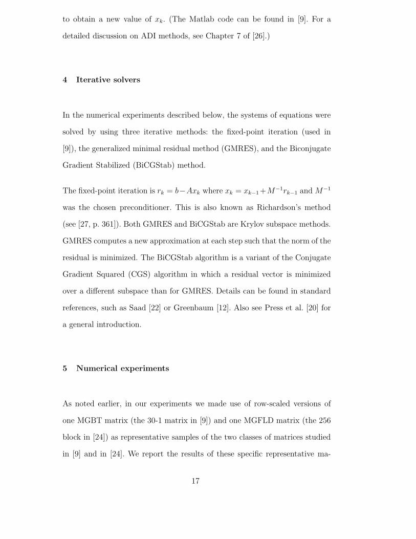
An examination of the actual inverse of the MGFLD matrix showed that the

dominant values were on diagonals spaced at 20 element intervals on either

side of the main diagonal (Fig. 2). Various SPAI preconditioners, all with

Fig. 2. The sparsity pattern of the dominant entries of a representative 200 × 200

block along the diagonal of the inverse of the MGFLD matrix.

a predetermined sparsity pattern, were tested in [24] with different numbers

of diagonals. The preconditioner that generally gave the best results in our

tests was a tridiagonal matrix with a main diagonal and additional diagonals

spaced 20 elements away on either side of the main diagonal. (Henceforth, we

refer to this matrix as the tridiagonal SPAI matrix.) The tridiagonal SPAI

18

matrix performed as well as a pentadiagonal and a 9-diagonal SPAI matrix

(both with the same diagonal spacing), and the computational overhead was

cheaper. As noted earlier, the convergence using the SPAI preconditioner from

the Barnard–Grote package was quite similar to the convergence using the

tridiagonal SPAI preconditioner.

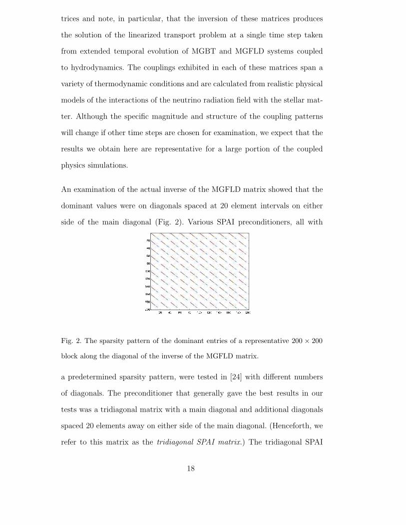
The actual inverse of the MGBT matrix, in contrast, did not reveal a pro-

nounced pattern that could be used to construct SPAI preconditioners (Fig.

3), unlike the case for the inverse of the MGFLD matrix. An SPAI precondi-

Fig. 3. The sparsity pattern of the dominant entries in the upper left corner,

mid-matrix, and lower right corner of the inverse of the MGBT matrix.

tioner obtained from the Barnard–Grote package was applied to the MGBT

matrix. With default values for the input tolerance, this preconditioner caused

the convergence to stagnate after a few iterations. In contrast, using the pre-

determined sparsity pattern of a 34 × 34 block diagonal matrix for our SPAI

preconditioner led to convergence, although at a slower rate than the ADI-like

preconditioner.

6 Results

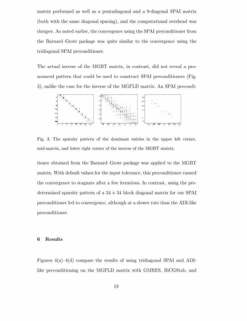
Figures 4(a)–4(d) compare the results of using tridiagonal SPAI and ADI-

like preconditioning on the MGFLD matrix with GMRES, BiCGStab, and

19

Richardson’s fixed-point iterative methods. For our numerical experiments,

the GMRES restart parameter was 30 (the Matlab default). An ADI-like pre-

conditioner for MGBT matrices, as described in [9], was effective. The same

preconditioner, suitably modified, was also effective for the MGFLD matrix

we investigated. In addition, we made use of the Barnard–Grote SPAI pack-

age to obtain an alternative SPAI matrix. It gave results comparable to those

from the tridiagonal SPAI preconditioner at the cost of additional overhead

to determine the sparsity pattern.

Since a flop count is dependent on the efficiency of an algorithm’s implemen-

tation and CPU timing is dependent on a platform’s user load, we decided

to make use of two invariant measures: the number of matrix-vector products

(“matvecs”) and the number of iterations. Both matvecs and iterations are

invariant across platforms and whether running an algorithm on a sequential

platform or in parallel.

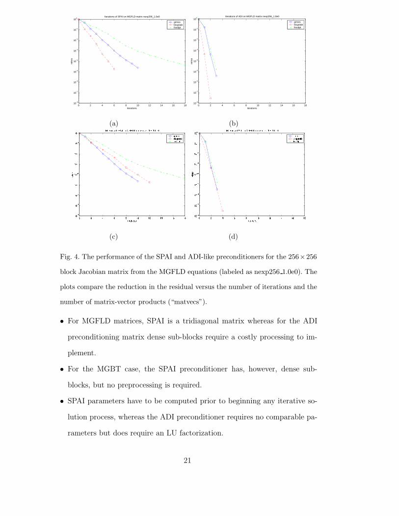
Figures 5(a)–5(d) compare ADI-like and block diagonal SPAI preconditioning

on the MGBT matrix also with GMRES, BiCGStab, and fixed-point itera-

tions. The plots show the apparent superiority of ADI-like preconditioning.

However, much of this apparent superiority derives from the tridiagonal solve

as was noted in Swesty et al. [24] where similar results were obtained without

the use of the costly block preconditioning step.

We note that the convergence behavior on display in Figure 5 shows stagnation

in the convergence of the SPAI preconditioned MGBT system. Stagnation

could be related to numerical singularity, rather than the SPAI preconditioner

per se.

Certain other features are important to note:

20

0 2 4 6 8 10 12 14 16 1810

−8

10−7

10−6

10−5

10−4

10−3

10−2

10−1

100

iterations

relre

s

Iterations of SPAI on MGFLD matrix nexp256_1.0e0

gmresbicgstabfixedpt

0 2 4 6 8 10 12 14 16 1810

−8

10−7

10−6

10−5

10−4

10−3

10−2

10−1

100

iterations

relre

s

Iterations of ADI on MGFLD matrix nexp256_1.0e0

gmresbicgstabfixedpt

(a) (b)

(c) (d)

Fig. 4. The performance of the SPAI and ADI-like preconditioners for the 256×256

block Jacobian matrix from the MGFLD equations (labeled as nexp256 1.0e0). The

plots compare the reduction in the residual versus the number of iterations and the

number of matrix-vector products (“matvecs”).

• For MGFLD matrices, SPAI is a tridiagonal matrix whereas for the ADI

preconditioning matrix dense sub-blocks require a costly processing to im-

plement.

• For the MGBT case, the SPAI preconditioner has, however, dense sub-

blocks, but no preprocessing is required.

• SPAI parameters have to be computed prior to beginning any iterative so-

lution process, whereas the ADI preconditioner requires no comparable pa-

rameters but does require an LU factorization.

21

0 5 10 15 20 25 3010

−8

10−7

10−6

10−5

10−4

10−3

10−2

10−1

100

iterations

relre

s

Iterations of SPAI on MGBT matrix 30−1

gmresbicgstabfixedpt

0 5 10 15 20 25 3010

−8

10−7

10−6

10−5

10−4

10−3

10−2

10−1

100

iterations

relre

s

Iterations of ADI on MGBT matrix 30−1

gmresbicgstabfixedpt

(a) (b)

(c) (d)

Fig. 5. The performance of the SPAI and ADI-like preconditioners for the 34 × 34

block Jacobian matrix from the MGBT equations (labeled as 30-1). The plots com-

pare the reduction in the residual versus the number of iterations and the number

of matrix-vector products (“matvecs”).

7 Conclusions

Our primary objective was to compare, on a sequential platform, the use of

two different preconditioners applied to linear systems involving two different

matrices related to similar physical phenomena. As has already been noted, the

original MGBT and MGFLD matrices, although similar in size and sparsity,

were significantly different in conditioning, but the scaled matrices used in our

tests were quite similar in their conditioning. We see our results as providing

22

motivation for additional work addressing issues beyond the scope of this

project, in particular, how an efficient implementation of the algorithms and

the preconditioners on a parallel machine would vary the results.

Figures 4 and 5 do not reflect the set-up and overhead time required to com-

pute the SPAI preconditioner. But these set-up and overhead times are, in fact,

quite minor since there is no cost associated with determining the sparsity pat-

tern of a predetermined pattern SPAI preconditioner and only the relatively

minor overhead of solving, for each row of the preconditioner, a k × n least

squares system where n is the number of non-zeros in that row of the pre-

conditioner and k the number of values taken from the corresponding rows of

the system matrix. Predetermined patterns, when they are identifiable, lead

to lower set-up and overhead costs, in comparison with the work needed for

the LU factorization of the dense diagonal blocks, which are necessary for the

ADI-like preconditioning.

Our tests do show the apparent success of using ADI-like preconditioning for

both MGBT and MGFLD matrices (using the schemes mentioned in §1 for

ordering the variables). For the MGBT matrix, the use of the SPAI precon-

ditioner results in a stagnation or very slow convergence, in comparison to

the use of the ADI-like preconditioner. For the MGFLD matrix, however, the

SPAI preconditioner did not stagnate, but converged steadily, yet at a some-

what slower rate than with the ADI-like preconditioner, no matter which of

the two measurements of matvecs or iterations was used.

The steady convergence leads us, therefore, to suggest that, for an MGFLD

matrix, the definite superiority of ADI-like preconditioning over SPAI is still

inconclusive. One of the reasons for this statement is the inherent advantage on

23

parallel platforms in the multiplication of matrices, a feature of SPAI precondi-

tioning, as compared to the backward and forward solves needed to implement

ADI-like preconditioners, even with improved parallel implementations. This

potential savings is not apparent in Figures 4 and 5 and, we suggest, is one

topic for future investigation.

We also believe our results encourage further studies with matrices of different

sizes to address questions related to the scalability of the two preconditioners

with either type of matrix. Some scalability tests were reported in [24, pp.

380–383] for SPAI preconditioners and three sizes of MGFLD matrices, and

these tests show essentially the same number of iterations needed for conver-

gence for all three sizes of matrices. Further studies are needed with ADI-like

preconditioners on MGFLD matrices and with the use of both preconditioners

on similarly-sized MGBT matrices.

Credits and Acknowledgements

The basic work on ADI-like preconditioners and MGBT matrices was done

by Eduardo D’Azevedo, Bronson Messer and others from Oak Ridge National

Laboratory. The basic work on SPAI preconditioners and MGFLD matrices

by Doug Swesty from SUNY Stony Brook in collaboration with Paul Saylor

(University of Illinois at Urbana-Champaign [UIUC]) and Dennis Smolarski

(Santa Clara University [SCU], while on leave at UIUC). Anthony Mezza-

cappa from Oak Ridge National Laboratory suggested a comparison between

the two different preconditioners on both MGBT and MGFLD matrices. The

comparison of the two preconditioners was done by Ramesh Balakrishnan,

John Fettig, Faisal Saied, Paul Saylor (all from UIUC) and Dennis Smolarski

24

(from SCU).

We also would like to thank Victor Eijkhout from the Texas Advanced Com-

puter Center at the University of Texas at Austin for discussions regarding

the ADI-like preconditioner for the MGBT matrices.

This work is supported by the Department of Energy SciDAC cooperative

agreement DE-FC02-01ER41185, www.phy.ornl.gov/tsi/. This research work

used the computational resources at the National Center for Supercomputing

Applications, www.ncsa.uiuc.edu.

References

[1] Alvarado, F. L., and Schreiber, R. (1993). Optimal parallel solution of sparse

triangular systems. SIAM J. Sci. Stat. Comput. 14, 446–460.

[2] Benzi, M., and Bertaccini, D. (2003). Approximate inverse preconditioning for

shifted linear systems, BIT 43, 231–244.

[3] Bethe, H., and Wilson, J. R. (1985). Revival of a stalled supernova shock by

neutrino heating, The Astrophysical Journal 295, 14–23.

[4] Bollhofer, M., and Mehrmann, V. (2002). Algebraic multilevel methods and

sparse approximate inverses, SIAM J. Mat. Anal. and Appl. 24, 191–218.

[5] Bollhofer, M., and Saad, Y. (2002). A factored approximate inverse

preconditioner with pivoting, SIAM J. Mat. Anal. and Appl. 23, 692–705.

[6] Bollhofer, M., and Saad, Y. (2002). On the relations between ILUs and factored

approximate inverses, SIAM J. Mat. Anal. and Appl. 24, 219–237.

[7] Chen, K. (2001). An analysis of sparse approximate inverse preconditioners for

boundary integral equations, SIAM J. Mat. Anal. and Appl. 22, 1058–1078.

25

[8] Chow, E. T.-F. (1997). Robust preconditioning for sparse linear systems, Ph.D.

thesis, The University of Minnesota.

[9] D’Azevedo, E. F., Messer, B., Mezzacappa, A., and Liebendoerfer, M. (2005).

An Adi-like preconditioner for Boltzmann transport, SIAM J. Sci. Comput. 26,

810–820.

[10] Golub, G. H., and C. F. V. Loan, C. F. F. (1996). Matrix Computations, 3rd

Edition, Johns Hopkins, Baltimore.

[11] Gould, H. I. M., and Scott, J. A. (1995). On approximate-inverse

preconditioners, Technical Report RAL 95-026, Computing and Information

Systems Department, Rutherford Appleton Laboratory, Oxfordshire, England.

[12] Greenbaum, A. (1997). Iterative Methods for Solving Linear Systems, SIAM,

Philadelphia.

[13] Grote, M. J., and Huckle, T. (1997). Parallel preconditioning with sparse

approximate inverses, SIAM J. Sci. Comput. 18, 838–853.

[14] Higham, N. J., and Pothen, A. (1994). The stability of partitioned inverse

approach to triangular solution. SIAM J. Sci. Stat. Comput. 15, 139–148.

[15] Liebendorfer, M. (2000). Consistent modelling of core-collapse supernovæ in

spherically symmetric relativistic space-time, Ph.D. Thesis, The University of

Basel.

[16] Messer, O. E. B. (2000). Questing for the grail: Spherically symmetric supernova

simulations with boltzmann neutrino transport, Ph.D. Thesis, The University

of Tennessee.

[17] Mezzacappa, A., and Bruenn, S. W. (1993). A numerical method for solving

the neutrino boltzmann equation coupled to spherically symmetric stellar core

collapse, The Astrophysical Journal 405, 669–684.

26

[18] Mezzacappa, A., and Messer, O. E. B. (1999). Neutrino transport in core

collapse supernovae, Journal of Computational and Applied Mathematics 109,

281–319.

[19] Mihalas, D., and Mihalas, B. W. (1984). Foundations of Radiation

Hydrodynamics, Dover, Mineola.

[20] Press, W. H., Teukolsky, S. A., Vetterling, W. T., and Flannery, B. P. (1992).

Numerical Recipes in Fortran 77, Cambridge University Press, Cambridge.

[21] Raghavan, P. (1998). Efficient parallel triangular solution with selective

inversion, Parallel Processing Letters, 8, 29–40.

[22] Saad, Y. (2003). Iterative methods for sparse linear systems, 2nd Edition, SIAM,

Philadelphia.

[23] Santos, E. E. (2000). On designing optimal parallel triangular solvers,

Information and Computation 161, 172–210.

[24] Swesty, F. D., Smolarski, D. C., and Saylor, P. E. (2004). A comparison of

algorithms for the efficient solution of the linear systems arising from multi-

group flux-limited diffusion problems, The Astrophysical Journal Supplement

Series 153, 369–387.

[25] Turner, N. J., and Stone, J. M. (2001). A module for radiation hydrodynamic

calculations with ZEUS-2D using flux-limited diffusion, The Astrophysical

Journal Supplement Series 135, 95–107.

[26] Varga, R. S. (1962). Matrix Iterative Analysis, Prentice–Hall, Englewood Cliffs.

[27] Young, D. M. (1971). Iterative Solution of Large Linear Systems, Academic

Press, New York.

27