on the order of accuracy and numerical performance of two ......on the order of accuracy and...
TRANSCRIPT
On the order of accuracy and numerical
performance of two classes of finite volume WENO
schemes∗
Rui Zhang†, Mengping Zhang‡and Chi-Wang Shu§
November 29, 2009
Abstract
In this paper we consider two commonly used classes of finite volume weightedessentially non-oscillatory (WENO) schemes in two dimensional Cartesian meshes.We compare them in terms of accuracy, performance for smooth and shockedsolutions, and efficiency in CPU timing. For linear systems both schemes arehigh order accurate, however for nonlinear systems, analysis and numerical sim-ulation results verify that one of them (Class A) is only second order accurate,while the other (Class B) is high order accurate. The WENO scheme in ClassA is easier to implement and costs less than that in Class B. Numerical exper-iments indicate that the resolution for shocked problems is often comparablefor schemes in both classes for the same building blocks and meshes, despite ofthe difference in their formal order of accuracy. The results in this paper maygive some guidance in the application of high order finite volume schemes forsimulating shocked flows.
Key Words: weighted essentially non-oscillatory (WENO) schemes; finite volumeschemes; accuracy
∗Dedicated to the memory of Professor David Gottlieb†Department of Mathematics, University of Science and Technology of China, Hefei, Anhui
230026, P.R. China. E-mail: [email protected]. Research supported in part by NSFC grant 10871190.‡Department of Mathematics, University of Science and Technology of China, Hefei, Anhui
230026, P.R. China. E-mail: [email protected]. Research supported in part by NSFC grant10671190.
§Division of Applied Mathematics, Brown University, Providence, RI 02912, USA. E-mail:[email protected]. Research supported in part by ARO grant W911NF-08-1-0520 and NSF grantDMS-0809086.
1

1 Introduction and the setup of the schemes
In this paper we are interested in numerically solving two dimensional conservationlaw systems
ut + f(u)x + g(u)y = 0 (1)
with suitable initial and boundary conditions, using the finite volume schemes onCartesian meshes. For this purpose, the computational domain is decomposed torectangular cells Ωij = [xi−1/2, xi+1/2] × [yj−1/2, yj+1/2], and for simplicity we assumethe mesh sizes ∆x = xi+1/2 − xi−1/2 and ∆y = yj+1/2 − yj−1/2 are constants. Thisassumption is not essential: finite volume schemes in this paper can be defined onarbitrary Cartesian meshes, even those with abrupt changes in mesh sizes, withoutaffecting their conservation, accuracy and stability. In a finite volume scheme we seekapproximations to the cell averages
¯ui,j =1
∆x∆y
∫ yj+1/2
yj−1/2
∫ xi+1/2
xi−1/2
u(x, y)dxdy. (2)
We use the notation u to denote the cell averaging operation in the x-direction (in-tegral in the cell [xi−1/2, xi+1/2] divided by the cell size ∆x), and u to denote the cellaveraging operation in the y-direction. The two dimensional cell average ¯u can beobtained by successively performing the cell averaging operators in x and in y. If weintegrate the conservation law (1) over the cell Ωij and then divide by its area, weobtain
d¯ui,j
dt+
1
∆x(fi+1/2,j − fi−1/2,j) +
1
∆y(gi,j+1/2 − gi,j−1/2) = 0 (3)
where ¯ui,j is the cell average (2) and
fi+1/2,j =1
∆y
∫ yj+1/2
yj−1/2
f(u(xi+1/2, y))dy (4)
gi,j+1/2 =1
∆x
∫ xi+1/2
xi−1/2
g(u(x, yj+1/2))dx (5)
are the physical fluxes, which are cell averages of f(u) in y at x = xi+1/2 and of g(u) inx at y = yj+1/2 respectively. Although (3) looks like a scheme, we should emphasizethat it is actually an equality satisfied by the exact solution of the PDE (1).
Notice that the equality (3) describes the evolution of the cell averages ¯ui,j whilerequiring the information of point values of the solution u in evaluating the physicalfluxes in (4) and (5). In order to convert the equality (3) to a scheme (commonlyreferred to as a finite volume scheme, since it solves for the cell averages ¯ui,j ratherthan point values of the solution) in the following form
d¯ui,j
dt+
1
∆x(fi+1/2,j − fi−1/2,j) +
1
∆y(gi,j+1/2 − gi,j−1/2) = 0, (6)
2
we must use a reconstruction procedure to obtain numerical fluxes fi+1/2,j and gi,j+1/2
in (6) as accurate approximations to the physical fluxes fi+1/2,j and gi,j+1/2 in (4) and(5).
We consider two classes of finite volume schemes in this paper. Both of themdepend crucially on the following one-dimensional reconstruction procedure.
One-dimensional reconstruction procedure: Given the cell averages
ui =1
∆x
∫ xi+1/2
xi−1/2
u(x)dx
of a piecewise smooth function u(x), the procedure uses these cell averages in sev-eral neighboring cells ui−`, · · · , ui+k (the collection of these neighboring cells is re-ferred to as the stencil of the reconstruction) to obtain an approximation to the pointvalue u(xi+1/2) at the cell interface or at another point u(x∗) where x∗ is in the cell[xi−1/2, xi+1/2]. We require the reconstruction to be high order accurate when u(x) issmooth in the stencil, and to be essentially non-oscillatory near discontinuities.
Such reconstruction procedure has been extensively studied in the literature,among high order ones we mention the essentially non-oscillatory (ENO) reconstruc-tion [2] and the weighted ENO (WENO) reconstruction [4, 3]. In the appendix we listthe fifth order WENO reconstruction procedure [3] that we use in this paper. Moredetails about WENO reconstruction can be found in, e.g. [7, 8, 5].
For a given physical flux f(u), based on monotonicity in the scalar case and oncharacteristic information and Riemann solvers in the system case, we can definea numerical flux f(u−, u+) where u− and u+ approximate the left and right limitsof the function u respectively. The numerical flux f(u−, u+) is at least Lipschitzcontinuous for both arguments, and is consistent with the physical flux in the sensethat f(u, u) = f(u). Examples of numerical fluxes for systems of conservation laws influid dynamics can be found in, e.g. [10, 6]. In this paper we use the Lax-Friedrichsflux and the HLLC flux as representative examples.
In the construction of finite volume schemes we often need to use a q-point Gaus-sian quadrature to approximate line integrals such as those (4) and (5):
fi+1/2,j ≈
q∑
k=1
ωkf(u(xi+1/2, ykj )), gi,j+1/2 ≈
q∑
k=1
ωkg(u(xki , yj+1/2)) (7)
where ωk are the Gaussian quadrature weights, and ykj and xk
i are the Gaussianquadrature points. In this paper we consider only schemes up to fifth order accuracy,hence q = 3 suffices.
We are now ready to define the two classes of finite volume schemes that we willstudy in this paper. The first class (Class A) of these methods has the followingalgorithm flowchart:
Finite volume scheme, Class A:
3
1. Using the two dimensional cell averages ¯ui,j, perform a one-dimensional recon-struction procedure in y to obtain a high order accurate approximation to thecell average of u in x at y = yj+1/2, denoted by ui,j+1/2. For the purpose of up-winding and stability, typically two different approximations, denoted by u−
i,j+1/2
and u+i,j+1/2, based on stencils biased to the left and to the right respectively,
are obtained.
2. Using the two dimensional cell averages ¯ui,j, perform a one-dimensional recon-struction procedure in x to obtain a high order accurate approximation to thecell average of u in y at x = xi+1/2, denoted by ui+1/2,j . Again, two differentapproximations, denoted by u−
i+1/2,j and u+i+1/2,j, based on stencils biased to the
left and to the right respectively, are obtained.
3. Form the numerical fluxes simply as
fi+1/2,j = f(u−
i+1/2,j , u+i+1/2,j), gi,j+1/2 = g(u−
i,j+1/2, u+i,j+1/2). (8)
4. Obtain the finite volume scheme (6), then discretize it in time by the TVDRunge-Kutta time discretization [9]. We use the third order version in thenumerical tests performed in this paper.
This finite volume scheme is very simple and efficient, and hence is widely used inapplications. However, this scheme is only second order accurate for general nonlinearsystems (systems in which the physical fluxes f(u) and g(u) are nonlinear functions ofu), regardless of the order of accuracy in the one-dimensional reconstruction procedureused in Steps 1 and 2 above. The problem arises in the choice of the numerical fluxesin Step 3 above. We will give a proof of this fact in the Appendix. Numericalexperiments in next section clearly demonstrate this second order accuracy. There ishowever an important exception. If the system is linear (that is, the physical fluxesf(u) = Au and g(u) = Bu where A and B are constant matrices), such as the linearMaxwell equations and linearized Euler equations, the same high order accuracy asin the one-dimensional reconstruction is achieved, see the Appendix for a proof andnext section for numerical verification.
The second class (Class B) of the finite volume methods that we will study in thispaper has the following algorithm flowchart:
Finite volume scheme, Class B:
1. Using the two dimensional cell averages ¯ui,j, perform a one-dimensional recon-struction procedure in y to obtain a high order accurate approximation to thecell average of u in x at y = yj+1/2, denoted by ui,j+1/2. For the purposeof upwinding and stability, typically two different approximations, denoted byu−
i,j+1/2 and u+i,j+1/2, based on stencils biased to the left and to the right respec-
tively, are obtained. This step is the same as the first step for the finite volumescheme in Class A.
4
2. Using the one dimensional cell averages u±
i,j+1/2, perform a one-dimensionalreconstruction procedure in x to obtain a high order accurate approximation tothe point values of u at the Gaussian quadrature points xk
i , denoted by u±
ik,j+1/2.
3. Using the two dimensional cell averages ¯ui,j, perform a one-dimensional recon-struction procedure in x to obtain a high order accurate approximation to thecell average of u in y at x = xi+1/2, denoted by ui+1/2,j . Again, two differentapproximations, denoted by u−
i+1/2,j and u+i+1/2,j, based on stencils biased to the
left and to the right respectively, are obtained. This step is the same as thesecond step for the finite volume scheme in Class A.
4. Using the one dimensional cell averages u±
i+1/2,j, perform a one-dimensionalreconstruction procedure in y to obtain a high order accurate approximation tothe point values of u at the Gaussian quadrature points yk
j , denoted by u±
i+1/2,jk.
5. Form the numerical fluxes using the Gaussian quadrature (7):
fi+1/2,j =
q∑
k=1
ωkf(u−
i+1/2,jk, u+
i+1/2,jk), gi,j+1/2 =
q∑
k=1
ωkg(u−
ik,j+1/2, u+ik,j+1/2).
(9)
6. Obtain the finite volume scheme (6), then discretize it in time by the TVDRunge-Kutta time discretization [9].
Comparing with the finite volume scheme in Class A, we can observe that thefinite volume scheme in Class B is more complicated and more costly, because of theadditional reconstructions in Steps 2 and 4 and the Gaussian quadrature sums in Step5. However, this scheme is genuinely high order accurate for nonlinear systems. Wewill give a proof of this fact in the Appendix. Numerical experiments in next sectionclearly demonstrate the high order accuracy.
2 Numerical experiments
We use the two dimensional Euler equations for compressible gas dynamics, namely(1) with
u =
ρρvρwE
, f(u) =
ρvρv2 + p
ρvwv(E + p)
, g(u) =
ρwρvw
ρw2 + pw(E + p)
,
where ρ is the density, (v, w) is the velocity, E is the total energy, E = pγ−1
+ 12ρ(v2 +
w2) where p is the pressure, with γ = 1.4 in our computation. The two classes
5
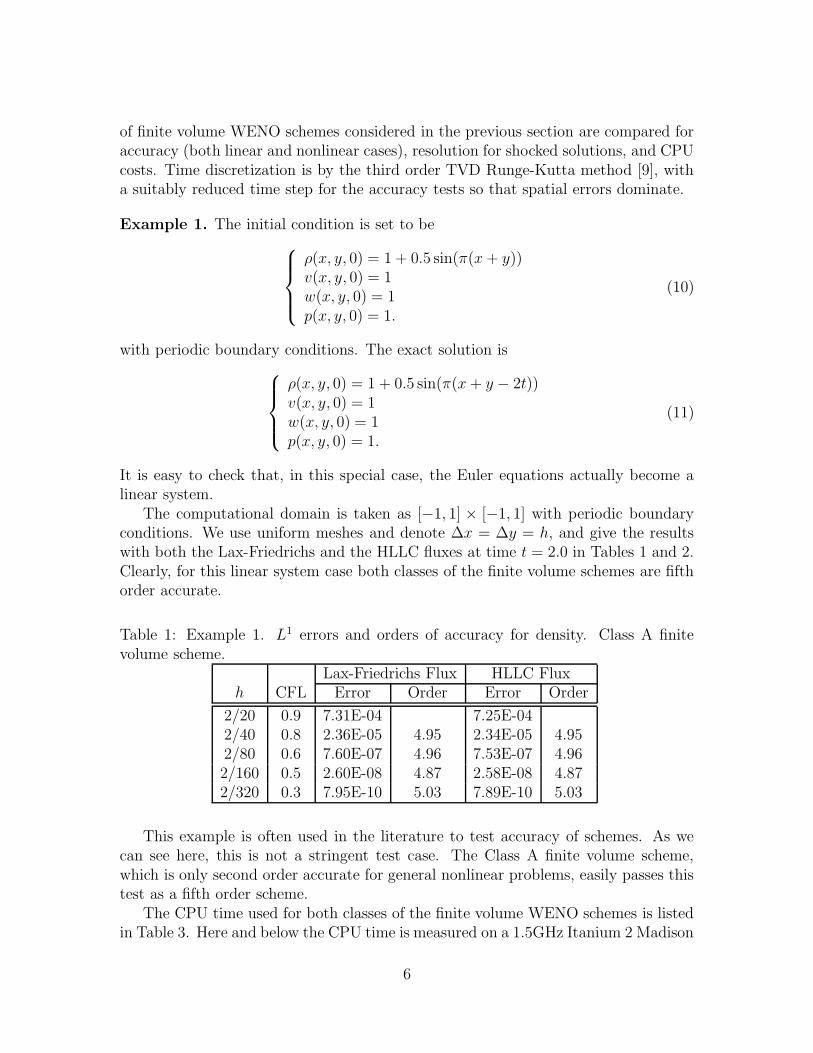
of finite volume WENO schemes considered in the previous section are compared foraccuracy (both linear and nonlinear cases), resolution for shocked solutions, and CPUcosts. Time discretization is by the third order TVD Runge-Kutta method [9], witha suitably reduced time step for the accuracy tests so that spatial errors dominate.
Example 1. The initial condition is set to be
ρ(x, y, 0) = 1 + 0.5 sin(π(x + y))v(x, y, 0) = 1w(x, y, 0) = 1p(x, y, 0) = 1.
(10)
with periodic boundary conditions. The exact solution is
ρ(x, y, 0) = 1 + 0.5 sin(π(x + y − 2t))v(x, y, 0) = 1w(x, y, 0) = 1p(x, y, 0) = 1.
(11)
It is easy to check that, in this special case, the Euler equations actually become alinear system.
The computational domain is taken as [−1, 1] × [−1, 1] with periodic boundaryconditions. We use uniform meshes and denote ∆x = ∆y = h, and give the resultswith both the Lax-Friedrichs and the HLLC fluxes at time t = 2.0 in Tables 1 and 2.Clearly, for this linear system case both classes of the finite volume schemes are fifthorder accurate.
Table 1: Example 1. L1 errors and orders of accuracy for density. Class A finitevolume scheme.
Lax-Friedrichs Flux HLLC Fluxh CFL Error Order Error Order
2/20 0.9 7.31E-04 7.25E-042/40 0.8 2.36E-05 4.95 2.34E-05 4.952/80 0.6 7.60E-07 4.96 7.53E-07 4.962/160 0.5 2.60E-08 4.87 2.58E-08 4.872/320 0.3 7.95E-10 5.03 7.89E-10 5.03
This example is often used in the literature to test accuracy of schemes. As wecan see here, this is not a stringent test case. The Class A finite volume scheme,which is only second order accurate for general nonlinear problems, easily passes thistest as a fifth order scheme.
The CPU time used for both classes of the finite volume WENO schemes is listedin Table 3. Here and below the CPU time is measured on a 1.5GHz Itanium 2 Madison
6
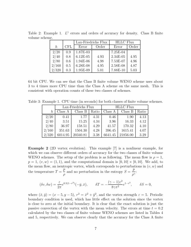
Table 2: Example 1. L1 errors and orders of accuracy for density. Class B finitevolume scheme.
Lax-Friedrichs Flux HLLC Fluxh CFL Error Order Error Order
2/20 0.9 1.87E-03 7.25E-042/40 0.8 6.12E-05 4.93 2.34E-05 4.952/80 0.6 1.94E-06 4.98 7.53E-07 4.962/160 0.5 6.28E-08 4.95 2.58E-08 4.872/320 0.3 1.95E-09 5.01 7.88E-10 5.03
64 bit CPU. We can see that the Class B finite volume WENO scheme uses about3 to 4 times more CPU time than the Class A scheme on the same mesh. This isconsistent with operation counts of these two classes of schemes.
Table 3: Example 1. CPU time (in seconds) for both classes of finite volume schemes.
Lax-Friedrichs Flux HLLC Fluxh Class A Class B Ratio Class A Class B Ratio
2/20 0.41 1.77 4.31 0.46 1.90 4.132/40 3.51 15.25 4.34 3.96 16.33 4.122/80 36.97 158.51 4.29 41.57 170.32 4.10
2/160 351.63 1504.30 4.28 396.45 1615.41 4.072/320 6014.95 20340.81 3.38 6641.45 21856.00 3.29
Example 2 (2D vortex evolution). This example [7] is a nonlinear example, forwhich we can observe different orders of accuracy for the two classes of finite volumeWENO schemes. The setup of the problem is as following. The mean flow is ρ = 1,p = 1, (v, w) = (1, 1), and the computational domain is [0, 10] × [0, 10]. We add, tothe mean flow, an isentropic vortex, which corresponds to perturbations in (v, w) and
the temperature T =p
ρand no perturbation in the entropy S =
p
ργ:
(δv, δw) =ε
2πe0.5(1−r2)(−y, x), δT = −
(γ − 1)ε2
8γπ2e1−r2
, δS = 0,
where (x, y) = (x − 5, y − 5), r2 = x2 + y2, and the vortex strength ε = 5. Periodicboundary condition is used, which has little effect on the solution since the vortexis close to zero at the initial boundary. It is clear that the exact solution is just thepassive convection of the vortex with the mean velocity. The errors at time t = 0.2calculated by the two classes of finite volume WENO schemes are listed in Tables 4and 5, respectively. We can observe clearly that the accuracy for the Class A finite
7
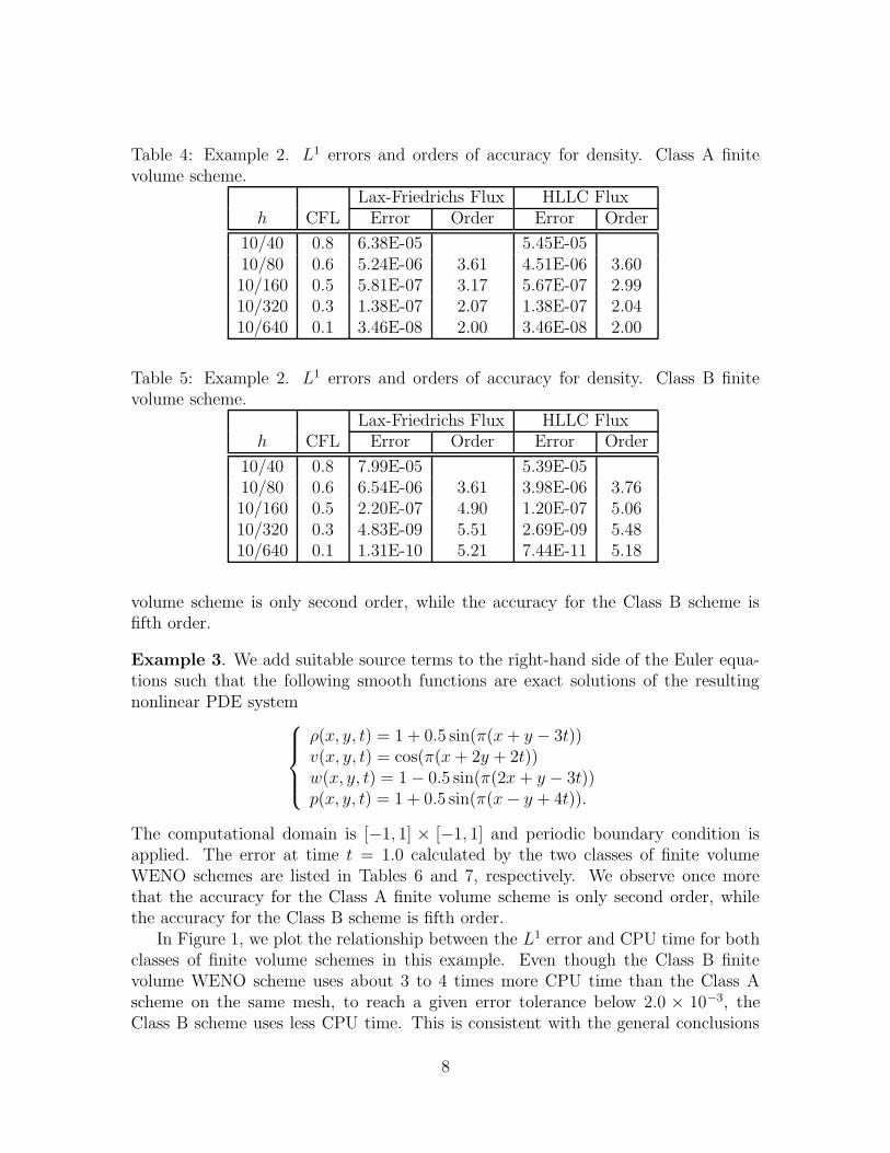
Table 4: Example 2. L1 errors and orders of accuracy for density. Class A finitevolume scheme.
Lax-Friedrichs Flux HLLC Fluxh CFL Error Order Error Order
10/40 0.8 6.38E-05 5.45E-0510/80 0.6 5.24E-06 3.61 4.51E-06 3.6010/160 0.5 5.81E-07 3.17 5.67E-07 2.9910/320 0.3 1.38E-07 2.07 1.38E-07 2.0410/640 0.1 3.46E-08 2.00 3.46E-08 2.00
Table 5: Example 2. L1 errors and orders of accuracy for density. Class B finitevolume scheme.
Lax-Friedrichs Flux HLLC Fluxh CFL Error Order Error Order
10/40 0.8 7.99E-05 5.39E-0510/80 0.6 6.54E-06 3.61 3.98E-06 3.7610/160 0.5 2.20E-07 4.90 1.20E-07 5.0610/320 0.3 4.83E-09 5.51 2.69E-09 5.4810/640 0.1 1.31E-10 5.21 7.44E-11 5.18
volume scheme is only second order, while the accuracy for the Class B scheme isfifth order.
Example 3. We add suitable source terms to the right-hand side of the Euler equa-tions such that the following smooth functions are exact solutions of the resultingnonlinear PDE system
ρ(x, y, t) = 1 + 0.5 sin(π(x + y − 3t))v(x, y, t) = cos(π(x + 2y + 2t))w(x, y, t) = 1 − 0.5 sin(π(2x + y − 3t))p(x, y, t) = 1 + 0.5 sin(π(x − y + 4t)).
The computational domain is [−1, 1] × [−1, 1] and periodic boundary condition isapplied. The error at time t = 1.0 calculated by the two classes of finite volumeWENO schemes are listed in Tables 6 and 7, respectively. We observe once morethat the accuracy for the Class A finite volume scheme is only second order, whilethe accuracy for the Class B scheme is fifth order.
In Figure 1, we plot the relationship between the L1 error and CPU time for bothclasses of finite volume schemes in this example. Even though the Class B finitevolume WENO scheme uses about 3 to 4 times more CPU time than the Class Ascheme on the same mesh, to reach a given error tolerance below 2.0 × 10⁻³, theClass B scheme uses less CPU time. This is consistent with the general conclusions
8
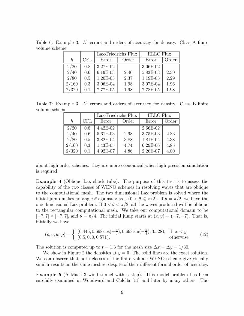
Table 6: Example 3. L1 errors and orders of accuracy for density. Class A finitevolume scheme.
Lax-Friedrichs Flux HLLC Fluxh CFL Error Order Error Order
2/20 0.8 3.27E-02 3.06E-022/40 0.6 6.19E-03 2.40 5.83E-03 2.392/80 0.5 1.20E-03 2.37 1.19E-03 2.292/160 0.3 3.06E-04 1.98 3.07E-04 1.962/320 0.1 7.77E-05 1.98 7.78E-05 1.98
Table 7: Example 3. L1 errors and orders of accuracy for density. Class B finitevolume scheme.
Lax-Friedrichs Flux HLLC Fluxh CFL Error Order Error Order
2/20 0.8 4.42E-02 2.66E-022/40 0.6 5.61E-03 2.98 3.75E-03 2.832/80 0.5 3.82E-04 3.88 1.81E-04 4.382/160 0.3 1.43E-05 4.74 6.29E-06 4.852/320 0.1 4.92E-07 4.86 2.26E-07 4.80
about high order schemes: they are more economical when high precision simulationis required.
Example 4 (Oblique Lax shock tube). The purpose of this test is to assess thecapability of the two classes of WENO schemes in resolving waves that are obliqueto the computational mesh. The two dimensional Lax problem is solved where theinitial jump makes an angle θ against x-axis (0 < θ 6 π/2). If θ = π/2, we have theone-dimensional Lax problem. If 0 < θ < π/2, all the waves produced will be obliqueto the rectangular computational mesh. We take our computational domain to be[−7, 7] × [−7, 7], and θ = π/4. The initial jump starts at (x, y) = (−7,−7). That is,initially we have
(ρ, v, w, p) =
(0.445, 0.698 cos(−π4), 0.698 sin(−π
4), 3.528), if x < y
(0.5, 0, 0, 0.571), otherwise(12)
The solution is computed up to t = 1.3 for the mesh size ∆x = ∆y = 1/30.We show in Figure 2 the densities at y = 0. The solid lines are the exact solution.
We can observe that both classes of the finite volume WENO scheme give visuallysimilar results on the same meshes, despite of their different formal order of accuracy.
Example 5 (A Mach 3 wind tunnel with a step). This model problem has beencarefully examined in Woodward and Colella [11] and later by many others. The
9

1e-007
1e-006
1e-005
0.0001
0.001
0.01
0.1
0.1 1 10 100 1000 10000 100000
Err
or
CPU time(seconds)
Class A WENOClass B WENO
1e-007
1e-006
1e-005
0.0001
0.001
0.01
0.1
0.1 1 10 100 1000 10000 100000
Err
or
CPU time(seconds)
Class A WENOClass B WENO
Figure 1: Example 3. L1 error versus CPU time for both classes of WENO schemes.Left: Lax-Friedrichs flux; Right: HLLC flux.
setup of the problem is the following. The wind tunnel is 1 length unit wide and 3length units long. The step is 0.2 length unit high and is located 0.6 length units fromthe left-hand end of the tunnel. The problem is initialized by a right going Mach 3flow. Reflective boundary conditions are applied along the walls of the tunnel andin-flow and out-flow boundary conditions are applied at the entrance (left-hand end)and the exit (right-hand end). For the treatment of the singularity at the corner ofthe step, we adopt the same technique used in [11], which is based on the assumptionof a nearly steady flow in the region near the corner. The numerical results are shown
in Figure 3, for the mesh sizes ∆x = ∆y =1
160and
1
320. We can observe that both
classes of the finite volume WENO scheme give visually similar results on the samemeshes, despite of their different formal order of accuracy.
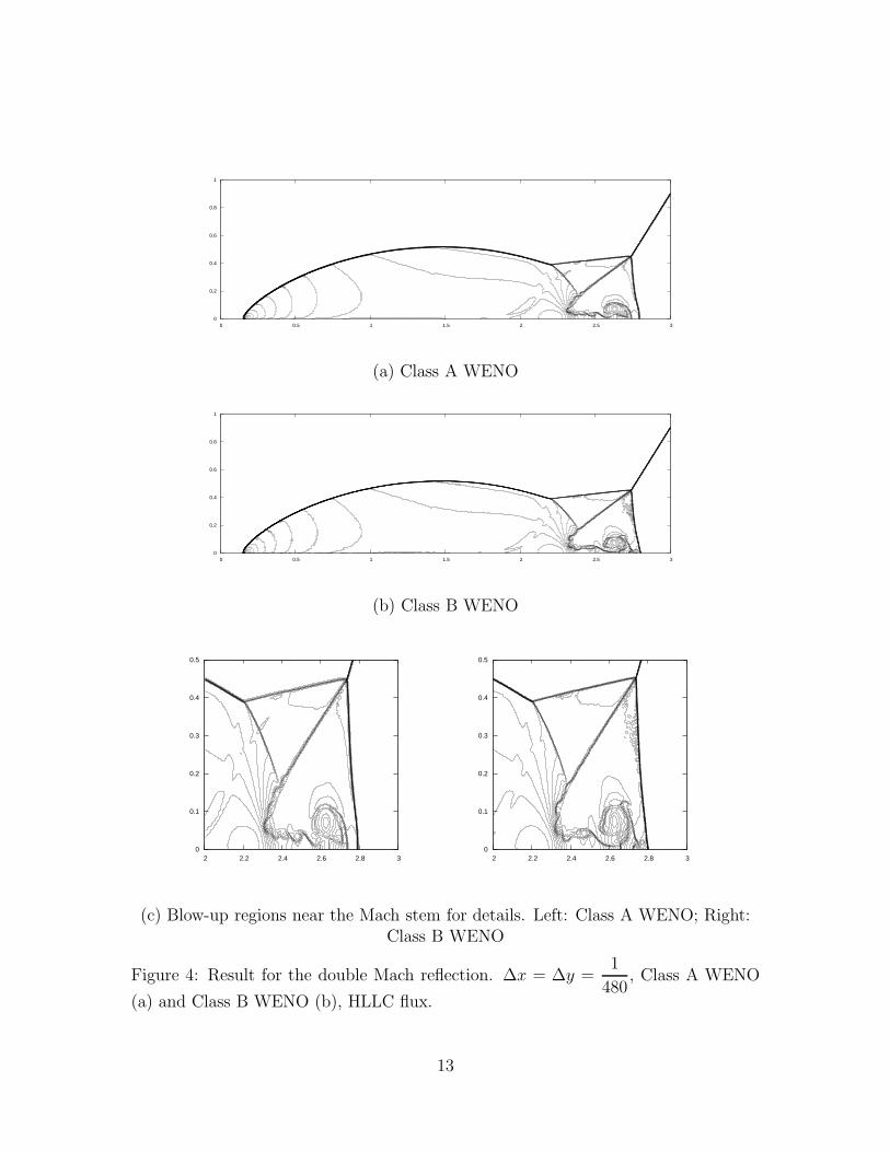
Example 6 (Double Mach reflection of a strong shock). The computational domainfor this problem is chosen to be [0, 4] × [0, 1]. The reflecting wall lies at the bottomof the computational domain starting from x = 1/6. Initially a right-moving Mach10 shock is positioned at x = 1/6, y = 0, and makes a 60 angle with the x-axis.For the bottom boundary, the exact postshock condition is imposed for the part fromx = 0 to x = 1/6 and a reflective boundary condition is used for the rest. At the topboundary of our computational domain, the flow values are set to describe the exactmotion of the Mach 10 shock. See [11] for a detailed description of the problem.
We give the results of both classes of the finite volume WENO schemes in Figure4 with ∆x = ∆y = 1/480. The results with ∆x = ∆y = 1/960 are given in Figure5. Again, we can observe that both classes of the finite volume WENO scheme givecomparable resolutions on the same meshes, despite of their different formal order ofaccuracy.
10

0.3
0.4
0.5
0.6
0.7
0.8
0.9
1
1.1
1.2
1.3
1.4
0 2 4 6 8 10 12 14 0.3
0.4
0.5
0.6
0.7
0.8
0.9
1
1.1
1.2
1.3
1.4
0 2 4 6 8 10 12 14
Figure 2: Oblique Lax shock tube. Density at y = 0. ∆x = ∆y = 1/30. Left: ClassA WENO; Right: Class B WENO.
3 Concluding remarks
Two classes of finite volume WENO schemes are discussed and tested in this paper.We observe numerically and prove theoretically that they are both high order accuratefor linear systems, however the Class A schemes are only second order accurate fornonlinear systems, while the Class B schemes are still high order accurate. Theoperation count and CPU timing for the Class B schemes are about 3 to 4 timesof those for the Class A schemes on the same mesh. However, for high precisionsimulation of smooth flows, Class B schemes could take less CPU time to reach thesame error threshold than Class A schemes. For problems with shocks, at least forthe test problems that we have experimented in this paper, the two classes of finitevolume schemes give comparable resolution on the same meshes, despite of theirdifference in formal order of accuracy. Results in this paper might shed some light onthe popularity of Class A schemes in applications.
A Appendix
In this appendix we describe briefly the fifth order WENO reconstruction procedure,and prove the orders of accuracy for the two classes of WENO schemes studied inthis paper.
11

0 0.5 1 1.5 2 2.5 3 0
0.1
0.2
0.3
0.4
0.5
0.6
0.7
0.8
0.9
1
(a) ∆x = ∆y = 1160
, Class A WENO
0 0.5 1 1.5 2 2.5 3 0
0.1
0.2
0.3
0.4
0.5
0.6
0.7
0.8
0.9
1
(b) ∆x = ∆y = 1160
, Class B WENO
0 0.5 1 1.5 2 2.5 3 0
0.1
0.2
0.3
0.4
0.5
0.6
0.7
0.8
0.9
1
(c) ∆x = ∆y = 1320
, Class A WENO
0 0.5 1 1.5 2 2.5 3 0
0.1
0.2
0.3
0.4
0.5
0.6
0.7
0.8
0.9
1
(d) ∆x = ∆y = 1320
, Class B WENO
Figure 3: Flow past a forward facing step. 30 contours from 0.1 to 6.6, Lax-Friedrichsflux.
12
0 0.5 1 1.5 2 2.5 3 0
0.2
0.4
0.6
0.8
1
(a) Class A WENO
0 0.5 1 1.5 2 2.5 3 0
0.2
0.4
0.6
0.8
1
(b) Class B WENO
2 2.2 2.4 2.6 2.8 3 0
0.1
0.2
0.3
0.4
0.5
2 2.2 2.4 2.6 2.8 3 0
0.1
0.2
0.3
0.4
0.5
(c) Blow-up regions near the Mach stem for details. Left: Class A WENO; Right:Class B WENO
Figure 4: Result for the double Mach reflection. ∆x = ∆y =1
480, Class A WENO
(a) and Class B WENO (b), HLLC flux.
13

0 0.5 1 1.5 2 2.5 3 0
0.2
0.4
0.6
0.8
1
(a) Class A WENO
0 0.5 1 1.5 2 2.5 3 0
0.2
0.4
0.6
0.8
1
(b) Class B WENO
2 2.2 2.4 2.6 2.8 3 0
0.1
0.2
0.3
0.4
0.5
2 2.2 2.4 2.6 2.8 3 0
0.1
0.2
0.3
0.4
0.5
(c) Blow-up regions near the Mach stem for details. Left: Class A WENO; Right:Class B WENO
Figure 5: Result for the double Mach reflection. ∆x = ∆y =1
960, Class A WENO
(a) and Class B WENO (b), HLLC flux.
14

A.1 Fifth order WENO reconstruction
We use the fifth-order WENO reconstruction procedure, described in [3]. Lower orhigher order reconstructions are also possible, see for example those in [4, 1].
For a piecewise smooth function v(x), we denote vi as its cell average. The fifth-order accurate reconstruction with a left-biased stencil is defined as
v−
j+1/2 = ω0v0 + ω1v1 + ω2v2 (13)
where vk are the reconstructed values obtained from cell averages in the k-th stencilSk = (j − k, j − k + 1, j − k + 2):
v0 =1
6(−vi+2 + 5vi+1 + 2vi),
v1 =1
6(2vi+1 + 5vi − vi−1),
v2 =1
6(11vi − 7vi−1 + 2vi−2)
(14)
and ωk, k = 1, 2, 3 are the nonlinear WENO weights given by
ωk =αk
∑3l=0 αl
, α0 =0.3
(ε + IS0)2, α1 =
0.6
(ε + IS1)2, α2 =
0.1
(ε + IS2)2. (15)
Here ε is a small parameter which we take as ε = 10−6 in our numerical tests. Thesmoothness indicators ISk are given by [3]
IS0 =13
12(vi − 2vi+1 + vi+2)
2 +1
4(3vi − 4vi+1 + vi+2)
2,
IS1 =13
12(vi−1 − 2vi + vi+1)
2 +1
4(vi−1 + vi+1)
2,
IS2 =13
12(vi−2 − 2vi−1 + vi)
2 +1
4(3vi−2 − 4vi−1 + 3vi)
2.
(16)
The right-biased reconstruction v+i+1/2 is obtained by symmetry with respect to the lo-
cation i+1/2. Reconstructions to values v(x∗) for x∗ inside the interval [xi−1/2, xi+1/2]can be obtained along the same lines, in fact only the formulas for the reconstructedvalues obtained from the small stencils in (14) and the linear weights (0.3, 0.6 and0.1) in (15) would change. We refer to, e.g. [5] for more details.
For the systems of conservation laws, a local characteristic decomposition is usedin the reconstruction. We refer to [3, 7] for more details.
A.2 Accuracy for the two classes of finite volume WENO
schemes
Theorem A.1. The Class B finite volume WENO scheme is accurate to the order
of accuracy of the reconstruction and quadrature rules.
15
Proof: We take as an example the case of a fifth order reconstruction and threepoint quadrature rules used in this paper. The proof for the general case is the same.The values u±
i+1/2,jkat the Gaussian points in (9) are reconstructed by the fifth-order
WENO procedure, which yields
u±
i+1/2,jk= u(xi+1/2, y
kj ) + O(∆x5 + ∆y5) (17)
where u(x, y) is the exact solution of the PDE (we have suppressed the t variable forsimplicity, as we are considering truncation errors in space only). Since the numericalflux f is Lipschitz continuous, we have
|f(u−
i+1/2,jk, u+
i+1/2,jk) − f(u(xi+1/2, y
kj ))|
= |f(u−
i+1/2,jk, u+
i+1/2,jk) − f(u(xi+1/2, y
kj ), u(xi+1/2, y
kj ))|
6 |f(u−
i+1/2,jk, u+
i+1/2,jk) − f(u−
i+1/2,jk, u(xi+1/2, y
kj ))|
+|f(u−
i+1/2,jk, u(xi+1/2, y
kj )) − f(u(xi+1/2, y
kj ), u(xi+1/2, y
kj ))|
6 L(|u+i+1/2,jk
− u(xi+1/2, ykj )| + |u−
i+1/2,jk− u(xi+1/2, y
kj )|)
= O(∆x5 + ∆y5).
(18)
The error for the 3-point Gaussian integration in (7) is
fi+1/2,j =3∑
k=1
ωkf(u(xi+1/2, ykj )) + O(∆y6). (19)
So we can get the error of the flux fi+1/2,j in (9) as
fi+1/2,j = fi+1/2,j + O(∆x5 + ∆y5) (20)
Assuming the leading term in the error O(∆x5 + ∆y5) in (20) is smooth, we have
1
∆x(fi+1/2,j − fi−1/2,j) −
1
∆x(fi+1/2,j − fi−1/2,j) = O(∆x5 + ∆y5). (21)
Similarly, we have
1
∆y(gi,j+1/2 − gi,j−1/2) −
1
∆y(gi,j+1/2 − gi,j−1/2) = O(∆x5 + ∆y5). (22)
We can see from (21) and (22) that the local truncation error for the Class BWENO scheme is fifth order.
Theorem A.2. The Class A finite volume WENO scheme is second order accurate
for general nonlinear conservation laws, but it is accurate to the order of the recon-
struction and quadrature rules for linear conservation laws with constant coefficients.
16
Proof: The values u±
i+1/2,j in (8) are reconstructed by the fifth order WENO proce-dure, hence we have
u±
i+1/2,j = ui+1/2,j + O(∆x5). (23)
By the Lipschitz continuity of the numerical flux f , we have
|fi+1/2,j − f(ui+1/2,j)| = |f(u−
i+1/2,j, u+i+1/2,j) − f(ui+1/2,j, ui+1/2,j)|
6 |f(u−
i+1/2,j, u+i+1/2,j) − f(u−
i+1/2,j, ui+1/2,j)|
+|f(u−
i+1/2,j, ui+1/2,j) − f(ui+1/2,j, ui+1/2,j)|
6 L(|u−
i+1/2,j − ui+1/2,j| + |u+i+1/2,j − ui+1/2,j|)
= O(∆x5).
(24)
That isfi+1/2,j = f(ui+1/2,j) + O(∆x5). (25)
Therefore we have
fi+1/2,j − fi−1/2,j
∆x=
f(ui+1/2,j) − f(ui−1/2,j)
∆x+ O(∆x5). (26)
Notice that the cell average of a function agrees with its value at the center of thecell to second order:
ui+1/2,j = u(xi+1/2, yj) + O(∆y2), (27)
andfi+1/2,j = f(u(xi+1/2, yj)) + O(∆y2), (28)
the combination of which gives
f(ui+1/2,j) = f(u(xi+1/2, yj) + O(∆y2))= f(u(xi+1/2, yj)) + O(∆y2).
(29)
We now havefi+1/2,j = f(ui+1/2,j) + O(∆y2), (30)
which is the crucial source of second order error regardless of the order of reconstruc-tion. We have, therefore,
1
∆x(fi+1/2,j − fi−1/2,j) −
1
∆x(fi+1/2,j − fi−1/2,j)
=1
∆x(fi+1/2,j − fi−1/2,j) −
1
∆x(f(ui+1/2,j) − f(ui−1/2,j)) + O(∆x5)
=1
∆x(fi+1/2,j − f(ui+1/2,j)) −
1
∆x(fi−1/2,j − f(ui−1/2,j)) + O(∆x5)
= O(∆x5) + O(∆y2)
(31)
where fi+1/2,j is defined with (8).
17
Similarly,
1
∆y(gi,j+1/2 − gi,j−1/2) −
1
∆y(gi,j+1/2 − gi,j−1/2) = O(∆x2) + O(∆y5). (32)
From (31) and (32) we can see that the scheme is only second order accurate.Now, if f(u) = Au is linear, then
∫ yj+1/2
yj−1/2
f(u(xi+1/2, y))dy = f
(
∫ yj+1/2
yj−1/2
u(xi+1/2, y)dy
)
, (33)
that is, instead of (30) we now have
fi+1/2,j = f(ui+1/2,j), (34)
thereby avoiding the crucial second order error. From (31) we can then get
1
∆x(fi+1/2,j − fi−1/2,j) −
1
∆x(fi+1/2,j − fi−1/2,j) = O(∆x5) (35)
which leads to fifth order in the local truncation error for this linear case.
References
[1] D.S. Balsara and C.-W. Shu, Monotonicity preserving weighted essentially non-
oscillatory schemes with increasingly high order of accuracy, Journal of Compu-tational Physics, 160 (2000), 405-452.
[2] A. Harten, B. Engquist, S. Osher and S. Chakravarthy, Uniformly high order
essentially non-oscillatory schemes, III, Journal of Computational Physics, 71(1987), 231-303.
[3] G.-S. Jiang and C.-W. Shu, Efficient implementation of weighted ENO schemes,Journal of Computational Physics, 126 (1996), pp.202-228.
[4] X.-D. Liu, S. Osher and T. Chan, Weighted essentially non-oscillatory schemes,Journal of Computational Physics, 115 (1994), 200-212.
[5] Y.-Y. Liu, C.-W. Shu and M. Zhang, On the positivity of linear weights in WENO
approximations, Acta Mathematicae Applicatae Sinica, 25 (2009), 503-538.
[6] J. Qiu, B.C. Khoo and C.-W. Shu, A numerical study for the performance of the
Runge-Kutta discontinuous Galerkin method based on different numerical fluxes,Journal of Computational Physics, 212 (2006), 540-565.
18

[7] C.-W. Shu, Essentially non-oscillatory and weighted essentially non-oscillatory
schemes for hyperbolic conservation laws, in Advanced Numerical Approximation
of Nonlinear Hyperbolic Equations, B. Cockburn, C. Johnson, C.-W. Shu and E.Tadmor (Editor: A. Quarteroni), Lecture Notes in Mathematics, volume 1697,Springer, Berlin, 1998, 325-432.
[8] C.-W. Shu, High order weighted essentially non-oscillatory schemes for convec-
tion dominated problems, SIAM Review, 51 (2009), 82-126.
[9] C.-W. Shu and S. Osher, Efficient implementation of essentially non-oscillatory
shock-capturing schemes, Journal of Computational Physics, 77 (1988), 439-471.
[10] E.F. Toro, Riemann Solvers and Numerical Methods for Fluid Dynamics, a Prac-
tical Introduction, Springer, Berlin, 1997.
[11] P. Woodward and P. Colella, The numerical simulation of two-dimensional fluid
flow with strong shocks, Journal of Computational Physics, 54 (1984), 115-173.
19