on the long term evolution of the spin of the earthaa.springer.de/papers/7318003/2300975.pdf · 976...

Astron. Astrophys. 318, 975–989 (1997) ASTRONOMYAND

ASTROPHYSICS

On the long term evolution of the spin of the EarthO. Neron de Surgy and J. Laskar

Astronomie et Systemes Dynamiques, Bureau des Longitudes, 3 rue Mazarine, F-75006 Paris, France

Received 6 November 1995 / Accepted 17 May 1996

Abstract. Laskar and Robutel (1993) have globally analyzedthe stability of the planetary obliquities in a conservative frame-work. Here the same model is extended by adding dissipativeeffects in the Earth–Moon system: the body tides and the fric-tion between the core and the mantle. Some constraints on thepoorly known coefficients of dissipation are determined withthe help of paleogeological observations. One consequence isthat the scenario proposed by Williams (1993) for the past his-tory of the Earth’s obliquity seems unlikely. A synthesis of 500numerical integrations of the Earth–Moon system with orbitalperturbations for the next 5 Gyr is presented. It is shown that thetime scale of the dissipative effects is long enough to induce anadiabatic–like evolution of the obliquity which is driven in thechaotic zone within 1.5 to 4.5 Gyr. A statistical study of pos-sible evolutions conducted with a tidal dissipation coefficient∆t of 600 seconds demonstrated that 68.4% of the trajectoriesattained an obliquity larger than 81 degrees, with a maximumof 89.5 degrees.

Key words: Earth – chaos – instabilities – celestial mechanics

1. Introduction

The recent works (Laskar et al., 1993a-b) and (Laskar and Robu-tel, 1993) emphasized the sensitivity of the obliquity εof a planetto the planetary perturbations. Indeed, secular resonances be-tween the precession motion of the rotation axis of a planet andthe slow secular motion of its orbit due to planetary perturba-tions can result in large chaotic variations of its obliquity. In thecase of the Earth, the presence of the Moon changes the Earth’sprecessing frequency by a large amount, and thus keeps it ina stable region, far from the large chaotic zone which resultsfrom secular resonances overlap (Laskar et al., 1993b). But dueto tidal dissipation, the Moon is slowly receding from the Earthand the Earth’s rotation is slowing down. Ultimately, the Earthwill reach the large chaotic zone due to planetary perturbations,and its obliquity will no longer be stable. The object of thepresent work is to provide a quantitative description of the longterm evolution of the Earth’s obliquity, in the future, but also inthe past.

The evolution of the Earth–Moon system is far from beinga new subject. Evidence of the loss of the Earth’s angular mo-mentum has long been observed through paleogeological clocks(for a review, see Williams, 1989), while the present deceler-ation of the lunar mean motion can be directly measured byLunar Laser Ranging (Dickey et al., 1994) with great precision.Nevertheless, accurate quantitative estimates of the length ofthe day over the age of the Earth are still lacking, and it is stilla difficult question to know the precise origins of these evolu-tions. Apart from the early work of (Darwin, 1880), the majorworks on the past history of the Earth-Moon system are dueto MacDonald (1964), Goldreich (1966) and Mignard (1979,1980, 1981). They found the same trends in the variations ofthe Earth’s spin and the lunar orbit due to the effects of thetides raised on the Earth by the Sun and the Moon. Adding theplanetary perturbations to the Earth’s orbit, Touma and Wis-dom (1994) recently confirmed those past variations, the ratesof which nevertheless remain uncertain because the coefficientof tidal dissipation is not well known. On the other hand, noneof these studies have taken into account the action of the frictionbetween the core and the mantle of the Earth as has been donein studies of Venus’ obliquity (see for example Goldreich andPeale, 1970, Lago and Cazenave, 1979, Dobrovolskis, 1980,Yoder, 1995). However, as is pointed out by Williams (1993),this effect could be of great importance, providing the spin withan obliquity decreasing with the time. The controversy aboutthe efficiency of the core–mantle friction arises from the factthat the possible effective viscosities of the outer core cover avery large range of values (Lumb and Aldridge, 1991), and inthe scenario presented by Williams (1993) for the past evolutionof the Earth’s obliquity, a very high value of this viscosity is as-sumed in order to obtain a past obliquity of the Earth reaching70 degrees one billion years ago.

On the other hand, the future of the evolution of the Earth’sobliquity has already been explored by Ward (1982) whichshowed, using a simple model with isolated resonances, thatthe precession frequency is expected to cross planetary secu-lar resonances in the future, which could allow the obliquityto increase up to 60 degrees. The reality is much more severe,as, from the extended work (Laskar et al.1993b) and (Laskarand Robutel, 1993), we know that as the Moon recedes fromthe Earth, as soon as the obliquity reaches the first important

976 O. Neron de Surgy & J. Laskar: On the long term evolution of the spin of the Earth

Fig. 1. The zone of large scale chaotic behavior for the obliquity ofthe Earth for a wide range of precession constant α (in arcseconds peryear). The non-hatched region corresponds to the stable orbits, wherethe variations of the obliquity are moderate, while the hatched zone isthe chaotic zone. The chaotic behavior is estimated by the diffusionrate of the precession frequency measured for each initial condition(ε, α) via numerical frequency map analysis over 36 Myr. In the largechaotic zones, the chaotic diffusion will occur on horizontal lines (α isfixed), and the obliquity of the planet can explore horizontally all thehatched zone. With the Moon, one can consider the present situation ofthe Earth to be represented approximately by the point with coordinatesε = 23.44, α = 54.93 ′′/yr, which is in the middle of a large zoneof regular motion. Without the Moon, for spin periods ranging fromabout 12h to 48h, the obliquity of the Earth would undergo very largechaotic variations ranging from nearly 0 to about 85. This figuresummarizes the results of about 250 000 numerical integrations of theEarth’s obliquity variations under perturbations due to the whole solarsystem for various initial conditions over 36 Myr. (Laskar and Robutel,1993, Laskar et al.1993b).

planetary secular resonance, it will enter a very large chaoticzone, with the possibility of attaining very high obliquities upto nearly 90 degrees.

Indeed, using Laskar’s method of frequency map analysisover more than 250 000 numerical integrations of the Earth’sobliquity for various values of the precession constant, it waspossible to obtain a clear picture of the global dynamics ofthe Earth’s obliquity (Laskar and Robutel, 1993) (Fig.1). Eachpoint of the graph represents one value of the couple (obliquity,precession constant), the precession constant being a quantityproportional to the speed of rotation (see formula (1) in Sect.2). One dot in the non-hatched zone corresponds to a stable po-sition, where the obliquity suffers only small (nearly quasiperi-odic) variations around its mean value, whereas one point inthe hatched zone corresponds to a chaotic behavior so that thehatched area delimits a region of resonances overlap where theEarth can wander horizontally. The present Earth is located in astable region (ε = 23.44 degrees, α = 54.93 arcsec/year), and the

present variations of the obliquity are limited to ±1.3 degreesaround its mean value (Laskar et al., 1993a).

Fig. 1 can be considered as a snapshot of the dynamics ofthe Earth’s obliquity, constructed in a conservative framework,over a relatively short time scale on which the dissipation dueto tidal interaction or core-mantle coupling is not yet visible.However, this picture already allows to forecast the future andpast evolutions of the Earth’s obliquity on much longer timescales, of several billions of years, when the various dissipativeeffects can no longer be neglected. Indeed, the consequence ofthis dissipation is to slow down the rotation of the Earth, so thatan initial point of the graph is slowly brought down to lowervalues of the precession constant. This suggests that the Earth’sspin has smoothly evolved since the formation or capture of theMoon. Our aim in the present work is to give a precise view of thefuture evolution of the Earth’s obliquity, and more specifically,to describe quantitatively its path in the chaotic zone.

The main limitation on a precise evolution of the Earth’srotational state is as much the crudeness and uncertainty of dis-sipative models as it is the values of their parameters, such asthe amplitude of the tidal dissipation, and even more, the vis-cosity of the outer core. The choice of the dissipative modeldoes not seem to be fundamental here, essentially because theEarth’s speed of rotation is not subject to large changes: differentmodels would not lead to very different variations, especiallywhen compared to the ones produced by planetary perturba-tions. Besides, in order to overcome difficulties arising from theuncertainty of the parameters, we will rely on the geological ob-servations of the length of the day (Williams, 1989). This willallow us to obtain a set of plausible values which correspondto these observations, and to fix the time scale of the evolutionalong the way.

Section 2 is devoted to determine the averaged equationsof secular rotational dynamics with planetary perturbations. InSect. 3 we present the chosen models for estimating the addi-tional dissipative contributions to these equations, while somelimits for the coefficients of dissipation will be obtained in Sect.4. Then we discuss in Sect. 5 the history of the Earth’s obliq-uity proposed by Williams (1993). Finally, we present in Sect.6 the results of a set of 500 numerical simulations of the futureevolution of the Earth for the next 5 Gyr, using Laskar’s methodof integration of the solar system (Laskar, 1988, 1994a), andstarting with very close initial conditions. Indeed, the chaoticnature of the motion prevents us from computing a single or-bit, and only a statistical approach becomes meaningful for thisproblem. Before concluding, we discuss some alternatives tothe results in relation to the coefficients of dissipation.

2. Averaged equations for the precession of the Earth withplanetary perturbations

The equations of precession of the Earth are derived from aHamiltonian function H which is the sum of the kinetic energyand of the potential energy Up of the torque exerted by the Sunand the Moon on the equatorial bulge of the Earth.

O. Neron de Surgy & J. Laskar: On the long term evolution of the spin of the Earth 977

Fig. 2. Reference frames for the definition of precession. Eqt and Ect

are the mean equator and ecliptic of the date with equinox γ. Ec0 isthe fixed J2000 ecliptic, with equinox γ0. i is the inclination of theecliptic Ect on Ec0. The general precession in longitude, ψ is definedby ψ = γN + Nγ0, where N is the ascending node of the ecliptic ofdate on the fixed ecliptic. ε is the obliquity, and ` = γA the hour angleof the equinox of date γ.

We suppose here that the Earth is an homogeneous rigidbody with moments of inertia A < B < C and we assumethat its spin axis is also the principal axis of inertia. It is con-venient here to use canonical Andoyer’s action variables (L,X)and their conjugate angles (`,−ψ) (Andoyer, 1923, Kinoshita,1977) (Fig. 2). L = Cω is the modulus of rotational angu-lar momentum of the Earth with rotation angular velocity ω;X = L cos ε, is the projection of the angular momentum on thenormal to the ecliptic, at obliquity ε; ` is the hour angle betweenthe equinox of the date γ and a fixed point of the equator; −ψthe opposite of the general precession angle (see Fig. 2).

Let (i, j, k) be a reference frame fixed with respect to theEarth, (I, J,K) a reference frame linked to the orbital plane ofthe perturbing body (Sun or Moon) around the Earth (see Fig.2), and R the rotation such that (i, j, k) = R(I, J,K).

According to Tisserand (1891) or Smart (1953) the potentialenergy of the torque exerted by a perturbing body P of mass Mat distance r from the Earth (E ), limited to its largest componentis

Up = −GMr

[A + B + C − 3I

2r2+ O

((Rr

)3)]

where R is the Earth’s radius. I denotes the Earth’s moment of

inertia around the radius vector r =−→E P, and is given by

I = A +1r2

(B − A)(r ·R(J))2 +1r2

(C − A)(r ·R(K))2 .

The motion of P around the Earth is determined by its el-liptical orbital elements defined with respect to the fixed eclip-tic Ec0 , with reference direction toward the fixed equinox γ0.Let us denote ω its argument of perigee, v its true anomaly,wd = Ω + ω + ψ + v the true longitude of date, where Ω isthe longitude of ascending node of the apparent orbit of P onEc0 if P is the Sun, and on Ect if it is the Moon.

We first build the precession equations due to the pertur-bation of the Sun only. When P is the Sun (subscript ), wehave:

r = r = r(

cos(ω + v)I + sin(ω + v)J)

and the transformation from the equatorial frame to the eclipticone (I, J,K) is:

R = R3(−ψ − Ω) R1(ε) R3(`) ,

where the rotations R1 and R3 are defined as

R1(θ) =

( 1 0 00 cos θ − sin θ0 sin θ cos θ

);

R3(θ) =

( cos θ − sin θ 0sin θ cos θ 0

0 0 1

).

Hence

1r2

(r ·R(J)

)2 = 14

[(1− cos 2` cos 2wd)(1 + cos2 ε )

+(cos 2wd − cos 2`) sin2 ε − 2 cos ε sin 2` sin 2wd]

1r2

(r ·R(K)

)2 = 12 sin2 ε (1− cos 2wd)

.

We retain only the contribution of terms with no sphericalsymmetry, which gives with Andoyer’s variables

Up =3Gm

4r3

(C − A)

(1− X2

L2

) (1− cos 2wd

)+

B − A2

[ (1− cos 2` cos 2wd

) (1 +

X2

L2

)+(

cos 2wd − cos 2`) (

1− X2

L2

)−2

XL

sin 2` sin 2wd

] .

Let M be the mean anomaly of the Sun. The fast angles `and wd are removed by taking the average

Up =1

2π

∫ 2π

0

(1

2π

∫ 2π

0Upd`

)dM,

unless a spin–orbit resonance occurs, i.e. when the angle` − k

2 M (k ∈ Z) is librating (Peale, 1969). This leads to thefollowing expression for the averaged potential due to the Sun:

Up = −3Gm4a3

C(1− e2)−3/2Ed

X2

L2

where Ed = (2C−A−B)/(2C) is called the dynamical elliptic-ity. The contribution of the Moon (subscript M) to the Hamil-tonian follows the same procedure with

r = rMRM(I)


where RM = R3(ΩM) R1(iM) R3(ωM + vM). Assuming aconstant rate for the precession of the orbit of the Moon (nodeand perihelion), one can also average the subsequent UpM on `,ΩM and MM , which gives:

UpM = −3GmM

4aM3

C(1− eM2)−3/2

(1− 3

2 sin2 iM)Ed

X2

L2

where iM is the inclination of the lunar orbit on the ecliptic.The full averaged Hamiltonian function of the described motionis then obtained by adding the rotational kinetic energy T =12 Cω2 = L2/2C, which gives

H =L2

2C− α

2X2

L

where α is the “precession constant”:

α =3G2ω

[m

(a√

1− e2)3+

mM

(aM√

1− eM2)3

(1− 32 sin2 iM)

]Ed

(1)

For a fast rotating planet like the Earth, Ed can be considered asproportional to ω2 ; this correspond to the hydrostatic equilib-rium (see for example Lambeck, 1980). In this approximation,α is proportional to ω.

Now, when considering the perturbations of the other plan-ets, the ecliptic Ect is not an inertial plane any more and thekinetic energy E of its driving has to be added. We refer here toKinoshita (1977).

Let (L?,X?, `?, ψ?) be Andoyer’s variables relative to thefixed ecliptic Ec0 , and (L,X, `, ψ) the variables relative to theecliptic Ect . Then (see for example Kovalevsky, 1963), if K is theHamiltonian of the system, function of the variables (L,X, `, ψ)relative to the moving Ect , and F the Hamiltonian written withthe variables (L?,X?, `?, ψ?) relative to Ec0 , the transformation

T : (L?,X?; `?,−ψ?) 7−→ (L,X; `,−ψ)

is canonical if, and only if, there exists a total differential formdW such that

Ld`+ Xd(−ψ)− L?d`? − X?d(−ψ?)− (K − F)dt = dW . (2)

The expression K − F is the searched energy E.In the previous section, H was the Hamiltonian F written

with the new variables (L,X, `, ψ). Then, the new HamiltonianK = E + H can be obtain by identifying E and dW in the Eq.(2). Thanks to Danjon (1959), one can establish the followingrelation:

cos(`? − `) = cos(−ψ − Ω) cos(−ψ? − Ω)

+ sin(−ψ − Ω) sin(−ψ? − Ω) cos i

where i is the inclination of Ect on the fixed plane Ec0 . Then, ifthe obliquity ε is oriented from the rotation axis k to the orbitnormal K, we have

d(`? − `) = cos ε d(−ψ − Ω)− cos ε? d(−ψ? − Ω)

− sin(−ψ − Ω) sin ε di

where ε? is the obliquity relative to Ec0 . As cos ε? = cos ε cos i+sin ε sin i cos(−ψ − Ω) (Danjon, 1959) and L = L?, we finallyobtain

Ld`− Xdψ − L?d`? + X?dψ?

−[(X(1− cos i)− L sin ε sin i cos(−ψ − Ω)]

dΩ

−L sin ε sin(−ψ − Ω) di = 0

which leads to

dW = 0

and

E =[(X(1− cos i) −L sin ε sin i cos(Ω + ψ)

] dΩdt

−L sin ε sin(Ω + ψ)di

dt

or

E = 2C (t)X − L√

1− X2

L2

(A(t) sinψ + B (t) cosψ

)with

A(t) =2√

1− p2 − q2

[q + p(qp− pq)

]B (t) =

2√1− p2 − q2

[p− q(qp− pq)

]C (t) = qp− pq

and where q = sin(i/2) cos Ω and p = sin(i/2) sin Ω.The canonical equations dX/dt = ∂K/∂ψ and dψ/dt =−∂K/∂X then give the precession equations on the form(Laskar, 1986, Laskar et al., 1993a-b):

dX

dt= L

√1− X2

L2

(B (t) sinψ −A(t) cosψ

)dψ

dt=αXL− X

L√

1− X2

L2

(A(t) sinψ + B (t) cosψ

)− 2C (t)

As was already done by Laskar et al.(1993b) and Laskar andRobutel (1993), since the contribution of the planetary pertur-bations to ψ is singular for ε = 0, we use for numerical integra-tions, instead of (X, ψ), the complex variable

χ = (1− cos ε)eiψ

which moves the singularity to ε = 180.A, B and C depend on fundamental frequencies of the

solar system and they are implicitly given by the integrationof the planetary motions. In this context, α is obviously not aconstant: e is also given by the integration of the solar system;ω, aM , eM and iM have to be determined as functions of timebecause of the dissipation.


3. Contributions of dissipative effects

Now we give estimations for the averaged contributions of thedissipation to dL/dt and dX/dt due to tides and core-mantleinteraction. For a review of the major features concerning theevolution of the Earth–Moon system, one can refer to the bookedited by Marsden and Cameron (1966). It helped us to delimitwhat was important for this study.

3.1. The body tides

One specific problem of modeling the dissipative tides on Earthis that they have two different origins: friction in the mantleand friction within shallow seas. The simplest way to overcomedifficulties and large formulae is to link the global dissipation toone physical quantity. In particular, this leads to consider herethe Earth, once again, as homogeneous.

The specific dissipation function Q (Munk and MacDon-ald, 1960) is often used. It is defined as the inverse of the ratio∆E/(2πE0) where ∆E is the energy dissipated during one pe-riod of tidal stress and E0 the maximum of energy stored duringthe same period. MacDonald (1964) showed that

Q−1 ' tan δ (3)

where δ is the phase lag of the deformation due to the stress.Q is rather considered as a constant (see for example Kaula,

1964, Goldreich and Peale, 1967, Goldreich and Soter, 1969,Gold and Soter, 1969), what implies in particular that δ is inde-pendent of the speed of rotation. This point remains subject tocontroversy, especially for long time scales. Some others stud-ies have also considered δ dependent of the tidal frequency:(Goldreich and Peale, 1966, 1970), (Lambeck, 1979), (Lagoand Cazenave, 1979), (Dobrovolskis, 1980). Most of them useFourier expansions of the tidal potential (Kaula, 1964) in whichan arbitrary tidal phase lag has to be defined for each argument,and the way these phase lags are related to the frequency is notalways clear. Moreover, relation (3) itself is subject to uncer-tainty as was pointed out by Zschau (1978).

As Touma and Wisdom (1994), we prefer here the simplerand more intuitive approach of Mignard (1979) where the torqueresulting of tidal friction is proportional to the time lag ∆t thatthe deformation takes to reach the equilibrium. This time lag issupposed to be constant, and the angle between the direction ofthe tide–raising body and the direction of the axis of minimalinertia (i.e. the direction of the high tide), which is carried outof the former by the rotation of the Earth, is proportional tothe speed of rotation. Such a model is called “viscous”, andcorresponds to the case for which 1/Q is proportional to thetidal frequency.

Theories on tidal effects are generally based on the follow-ing assertion mainly due to Love at the beginning of the century(see Lambeck, 1988): the tidal potential due to the deformationinduced by the differential gravitational attraction of a perturb-

ing body (the Sun or the Moon) at r∗ from the Earth’s center Oholds, at any point P on its surface:

V (r∗,R) =∑i≥2

kiVi(r∗,R),

where R =−→OP of which the modulus is the planetary radius R,

where ki the ith Love number and Vi the ith spherical harmonic.As was done for the computation of the potential of precession,we restrict ourselves to the first term of the expansion, whatseems to be sufficient for estimating secular variations. Hence

V (r∗,R) = k2V2(r∗,R) = −Gm∗k2

2r∗5

(3(R · r∗)2 − R2r∗2) (4)

The potential V at any point outside the Earth of distance r′ is thesolution of the “Dirichlet’s first boundary–value problem” (seeLambeck, 1988), so to say that it satisfies Laplace’s equation

∇2V = 0

and its value V (r∗,R) on the boundary of the domain r′ > R isknown and given by Eq. (4). The unique solution to this problemis the function

V (r∗, r′) = k2

(Rr′)5

V2(r∗, r′).

Here r∗ stands for the perturbing body and r′ for the in-teracting body at time t. r∗ would also be defined at time t ifthe Earth were perfectly elastic. But this is not the case since,due to internal friction, the deformation permanently takes atime ∆t to reach the equilibrium; the attribute (∗) referring tothe perturbing body also means that the value is taken at timet −∆t.

Assuming∆t small compared to the diurnal period, Mignardgives the following approximation for the perturbing body:

r∗ = r(t −∆t) +−→ω ∆t × r = r + (−→ω × r − v)∆t

where v is the orbital velocity, −→ω the rotational velocity, andwhere all vectors in the right member are defined at time t. ThenMignard expands V at first order in ∆t and derives the force Fand torque Γ undergone by the interacting body:

F = −m′gradr′V = 3Gm∗m′R5k2∆t

r′5r5×

5

r′2

[(r′ · r)

[r · (−→ω × r′) + r′ · v

]− 1

2r2(r · v)

[5(r′ · r)2 − r′2r2

]]r′

−[r · (−→ω × r′) + r′ · v]r

−(r′ · r)[r ×−→ω + v

]+

r · v

r2

[5(r′ · r)r − r2r′

],


Γ = r′ × F = −3Gm∗m′R5k2∆t

r′5r5×[[

r · (−→ω × r′) + r′ · v] − 5

r · v

r2(r′ · r)

](r′ × r)

+(r′ · r)[(r′ · −→ω )r − (r′ · r)−→ω + r′ × v

].

The determination of Γ gives the contribution of the bodytides to the variation of the spin:

dL

dt= − 1

ωΓ · −→ω

dX

dt= −Γ · K

where K is the normal to the ecliptic.We have computed Γ with the help of the algebraic manip-

ulator TRIP (Laskar, 1994b), writing all vectors in ecliptic co-ordinates and averaging both formula over the periods of meananomaly, longitude of node and perigee of the perturbing body(and of the interacting body if it is not the same one). Takingsecond order truncations in eccentricities, we obtain:

• the contributions of the solar tides (r′ = r = r):

dL

dt= −3Gm2

R5k2∆t

2a6×

[(1 + 15

2 e2)(

1 +X2

L2

) LC− 2(1 + 27

2 e2)XL

n

]dX

dt= −3Gm2

R5k2∆t

2a6×[

2(1 + 15

2 e2)X

C− 2(1 + 27

2 e2)n

]where n is the mean motion of the Sun around the Earth.

• the contributions of the lunar tides (r′ = r = rM):

dL

dt= −3Gm2

MR5k2∆t

2a6M

×[

12

(1 + 15

2 eM2)[

3− cos2 iM + (3 cos2 iM − 1)X2

L2

] LC

−2(1 + 272 eM

2)XL

nM cos iM

]dX

dt= −3Gm2

MR5k2∆t

2a6M

×[(1 + 15

2 eM2)(1 + cos2 iM)

XC

−2(1 + 272 eM

2) nM cos iM

]• the contributions of the “cross tides” (r′ = rM and r =

r ; r′ = r and r = rM), the cases where the Moon and the

Sun are respectively the perturbing bodies accounting for thesame quantity:

dL

dt= −3GmmMR5k2∆t

4a3aM3

×

(1 + 3

2 e2)(

1 + 32 eM

2)(3 cos2 iM − 1)

(1− X2

L2

) LC

dX

dt= 0

Let us have a look on the consequences of all these contribu-tions. Neglecting the eccentricities, the variation of the obliquitydue to the direct solar tides or the lunar ones with a low incli-nation of the Moon has the form:

dx

dt= k(x2 − 1)( 1

2ωx − n)

where x = cos ε and k is a positive quantity. This implies thatε = 0 and ε = 180 are two instable positions of equilibriumand that ε = arccos( 2n

ω ) = ε0 is a stable position, but it isa relative stability because the braking of L makes it slowlymoves down to 0. Furthermore, the obliquity increases whenε < ε0 and decreases otherwise.

It is easy to see that the cross tides drive the equator to-wards the orbital plane. They are missing in Mignard’s articlesbut Touma and Wisdom (1994) have pointed out their relativeimportance. Actually, the ratio of their magnitude with the oneof the direct solar tides (21.6% of the lunar one) is

mMa3

2maM3' 1.1 .

As dL/dt is proportional to sin2 ε , this contribution must betaken into account whenever the obliquity reaches high values.

We can derive now from F the variations of the orbit of theinteracting body induced by the tides. They can be obtained bydetermining the components R′, S′ and W ′ of F in an osculatingreference frame. These components write:

R′ =1µr′

F · r′ ,

S′ =1

H ′µr′F · (H′ × r′) ,

W ′ =1

H ′µF · H′,

where µ is the so–called reduced mass of the system Earth-interacting body and H′ the orbital angular momentum of theinteracting body:

µ =m⊕m′

m⊕ + m′ ; H ′ = m′n′a′2√

1− e′2.


The orbital variations are given by the Lagrange equations(see Brouwer and Clemence, 1961):

da′

dt=

2

n′√

1− e′2

[R′e′ sin v′ + S′

a′

r′(1− e′2)

]de′

dt=

√1− e′2

n′a′e′[R′e′ sin v′ + S′

(a′

r′(1− e′2)− r′

a′)]

di′

dt=

r′ cos w′

n′a′2√

1− e′2W ′

where v′,w′, i′ are respectively the true anomaly, the longitudeof perigee and the inclination of the interacting body on theecliptic Ect . After expanding and averaging these equations andtaking second order truncations in eccentricity, we find for theMoon:

daM

dt=

6GmM2R5k2∆t

µaM7

×[(

1 + 272 eM

2) X

CnMcos iM − (1 + 23eM

2)]

deM

dt=

3GmM2R5k2∆t eM

µaM8

[112

XCnM

cos iM − 9]

dcos iMdt

=3GmM

2R5k2∆t2µaM

8(1 + 8eM

2)X

CnMsin2 iM

(5)

and for the Sun:dadt

=6Gm2R5k2∆t

m oa7

[(1 + 27

2 e2) X

Cn− (1 + 23e2)

]dedt

=3Gm2R5k2∆t e

ma8

[112

XCn

− 9]

but both last variations are negligible: about 3 meters per Myrfor da/dt and 10−12 per Myr for de/dt.

Two contributions are missing so far: the tides raised on theMoon by the Earth and by the Sun. With the following assump-tions:a) The inclination of the Moon’s equator on its orbital plane is

small (6.41 at this time), so we can use the approximationsεM ' 0 and i′ ' 0,

b) The Moon is locked in synchronous spin–orbit resonance1:1 with the Earth (i.e. ωM = nM),the tide raised by the Moon on the Earth is obtained by

exchanging Moon and Earth in Eqs. (5) with the above simpli-fications. We obtain the additional contributions:

daM

dt= −57Gm⊕2RM

5k2M∆tMeM2

µaM7

deM

dt= −21Gm⊕2RM

5k2M∆tMeM

2µaM8

If one takes k2M∆tM ' 213 suggested by the DE245 data,k2 = 0.305 (Lambeck, 1980), and ∆t = 638 seconds, these

contributions represent 1.2% of the total daM/dt and 30% ofthe total deM/dt for present conditions. As Mignard pointed itout, the terrestrial tides on the Moon have no substantial effecton the lunar orbit unless it is close to the Earth (at a few Earth’sradii) and when the ratio k2M∆tM/(k2∆t) is much greater than1 (using DE245 data, we have ρ ' 1.1).

Finally, the tides raised on the Moon by the Sun can alsobe neglected because the ratio of the magnitudes of solar andterrestrial tides on the Moon is(m

m⊕

)2(aaM

)6' 3.2× 10−5.

3.2. The core–mantle friction

Here we basically rely on Rochester’s model (1976).The inner Earth is composed of a mantle and a core separated

into a central rigid part and a fluid one. We neglect interactionsbetween both last parts because they are supposed to be stronglycoupled by pressure forces (Hinderer, 1987). The core and themantle have different dynamical ellipticities, so they tend tohave different precession rates. This trend produces a viscousfriction at the core–mantle boundary (CMB). Thus, there aremotions in the outer liquid core inducing electric currents whichgenerate a torque of electromagnetic friction because of mag-netization of the deepest layer of the mantle.

Rochester showed that the magnetic friction has only a fainteffect on the Earth’s long term rotational dynamics. If the co-efficient of viscous friction due to the viscosity of the liquidmetal of the outer core is thought weaker that the magnetic one,some turbulences and inhomogeneıties in the outer core couldmake the viscous friction far more efficient (Lumb and Aldridge,1991), (Williams, 1993), so that we will suppose that the fric-tion is solely viscous. We will consider here that an effectiveviscosity ν can account for a weak laminar friction, as well asa strong turbulent one which thickens the boundary layer.

Two additional torques account for the coupling: the inertialtorque N due to pressure forces at the CMB (which is not spher-ical due to the Earth’s rotation) , and the topographic torque(Hide, 1969) due to likely “bumps” of this boundary. N tends toattach strongly the core and the mantle but its effect is reducedif the boundary layer beneath the CMB is thick. Although irreg-ularities of the CMB increase the surface of friction, this topo-graphic torque (which is not taken into account in Rochester’smodel) would rather have a conservative effect, the bumps act-ing as notches; in this way it can be considered as the irregularpart of N. Besides, it is still too poorly known to estimate its longterm contributions (Jault, private communication). We will alsoignore it.

The angular momentum theorem applied to the core (sub-script c) and to the mantle (subscript m) then gives:

d(Cc−→ωc )

dt= Pc + N + F

d(Cm−→ωm)

dt= Pm − N − F

(S)


where Pc, Pm are the precession torques, and F the frictionaltorque. Cc and Cm denote the moment of inertia with C = Cc +Cm. In first approximation, one can write:

F = κ (−→ωm −−→ωc ) = κ−→δ

where κ is the effective coefficient of friction. Rochester givesthe following approximation to the solution of system (S):

dε

dt= −κψ

2 sin ε cos ε

γelEd c2Cω2

where γel is the elasticity correcting factor of the mantle andψ the Earth’s rate of precession. Ed c is the dynamical elliptic-ity of the core which, as the whole body one, is assumed to beproportional to the square of the speed of rotation. It shouldnot differ from the value corresponding to the hydrostatic equi-librium by more than a few percents (Hinderer, 1987). HenceEd = Ed inω

2/ωin2 and Ed c = Ed cin

ω2/ωin2. where the subscript

in denotes the initial value. As pointed out by Yoder (1995),such approximations would not be valid any more for a slowrotation, for which the non-hydrostatic parts of the ellipticitiescan dominate.

This solution is valid only when the inertial torque N is non–zero. This happens when the ellipticity of the CMB exceeds theratio of the rotation period to the precession period (Poincare,1910, see also Peale, 1976). Assuming that this ellipticity isroughly in hydrostatic equilibrium, this condition is equivalentto:

ω >(πGρc | ψ |

)1/3, (C)

where ρc is the density of the outer core. The rate ψ beingproportional toω (see Sect. 2), such a condition is satisfied sinceω exceeds a given constant; this is the case for a fast–rotatingplanet like the Earth.

We determine κ as a function of the effective viscosity withthe help of Goldreich and Peale (1967, 1970). First, we computethe “spin-up” time which corresponds to the time that the coreneeds to adjust its rotation to the one of the mantle in absenceof any external force. This is the characteristic time τ of thefollowing system:

d(Cm−→ωm)

dt= −F = −κ−→δ

d(Cc−→ωc )

dt= F = κ

−→δ

The solution is

−→δ =

−→δ0 e−t/τ , τ =

CcCm

κC.

Thus, according to Greenspan and Howard (1963),

τ =Rc√νω

.

Hence

κ =CcCm

√νω

CRc

what yields

dε

dt= −CcCmψ

2√ν cos ε sin ε

γelC2RcEd c2ω3/2

i.e.

dcos ε

dt=

CcCmψ2√ν

γel

√CRcEd c

2

(1− X2

L2

) X

L5/2.

The contributions of the core–mantle friction to dL/dt anddX/dt are obtained thanks to the fact that −→ωc is very close to−→ωm because of the action of N. Then the precession torques Lm

and Lc belonging to the orbital plane of normal K (this clearlyappears when the torques are expressed in a vectorial form; seefor example Goldreich 1966), the addition of both equations of(S) and the scalar product by K of the resulting equation leadsto

dX

dt' 0,

which implies

dL

dt= − CcCmψ

2√νγel

√CRcEd c

2

(1− X2

L2

) 1L1/2

.

This quantity being always negative, the core–mantle friction(CMF) tends to slow down the rotation and to bring the obliquitydown to 0 if ε < 90 and up to 180 otherwise, what contrastswith the effect of the tides. Furthermore, one can see that, despitethe strong coupling by pressure forces, there can be a substantialcontribution to the variation of the spin for high viscosities andmoderate speeds of rotation. It must be pointed out that thiscontribution has no sense for an arbitrary high viscosity (whichwould attach the core to the mantle) and for an arbitrary smallcore dynamical ellipticity (for which N vanishes).

Finally, the equation dX/dt = 0 has also the followingremarkable consequence: since

dcos ε

dt=

1L

(dX

dt− X

L

dL

dt

),

we havedLL

= −d cos εcos ε

what yields∫ t2

t1

dωω

= −∫ t2

t1

d cos εcos ε

i.e.ω(t1)ω(t2)

=cos ε (t2)cos ε (t1)

(R)

This simple relation is independent of the variations of ν andstrongly constraints the possible evolution of ε.


3.3. The atmospheric tides

The Earth’s atmosphere also undergoes some torques whichcan be transmitted to the surface by friction: a torque caused bythe gravitational tides raised by the Moon and the Sun, a mag-netic one generated by interactions between the magnetosphereand the solar wind. Both effects are negligible; see respectivelyChapman and Lindzen (1970) and Volland (1988).

Finally, a torque is produced by the daily solar heating whichinduces a redistribution of the air pressure, mainly driven bya semidiurnal wave, hence the so-called thermal atmospherictides (Chapman and Lindzen, 1970). The axis of symmetry ofthe resulting bulge of mass is permanently shifted out of thedirection of the Sun by the Earth’s rotation. As for the bodytides, this loss of symmetry is responsible for the torque which,at present conditions, tends to accelerate the spin.

Volland (1988) showed that this effect is not negligible, re-ducing the Earth’s despinning by about 7.5%. But, although theestimate of their long term contributions surely deserves carefulattention, we have not taken the atmospheric tides into accountin the computations presented in the next sections, assumingthat, as the uncertainty on some of the other factors is still im-portant, the global results obtained here will not differ muchwhen taking this additional effect into consideration.

4. Some limits to the coefficients of dissipation

Goldreich (1966), Mignard (1979, 1980, 1981) and Touma andWisdom (1994) have studied the past evolution of the Earth–Moon system taking the distance of the Moon to the Earth asthe independent variable instead of the time. This is because ifone takes the present value ∆t = 638 seconds which fits theobserved receding of the Moon for which Dickey et al. (1994)give 3.82 cm per year, it is found that the capture or formation ofthe Moon occurred at about −1.2 Gyr which contradicts mostof paleogeological observations (see for example Piper, 1978,Lambeck, 1980).

So ∆t has clearly been smaller in the past, probably be-cause of the changes in the continental distribution (Krohn andSundermann, 1978) and in the oceanic loading during glacia-tions. We only need for our purpose to consider some acceptableaverage value anyway.

With a review of experiments in laboratories and observa-tions of fluctuations of the Earth’s spin, Lumb and Aldridge(1991) give a range of possible values for the effective viscosityν going from 10−7 up to 4.6 × 105 m2s−1. Although the influ-ence of the friction is proportional to

√ν, the uncertainty about

the effect of internal friction still remains a serious problem.Rochester has chosen to set the upper limit to 10 m2s−1 whichcomes from observations of the fluctuations of the Earth’s nu-tation (Toomre, 1974). Actually this last value changes the spinvery little. On the opposite, Williams asserts that ν should bemuch larger. This comes out from his assessment of observa-tions of sediments and fossils which suggests that the historyof the obliquity would have been very different from the con-sensual one, starting from 70 and going down to the present

2327′ with a drastic falldown at about −630 Myr (Williams,1993).

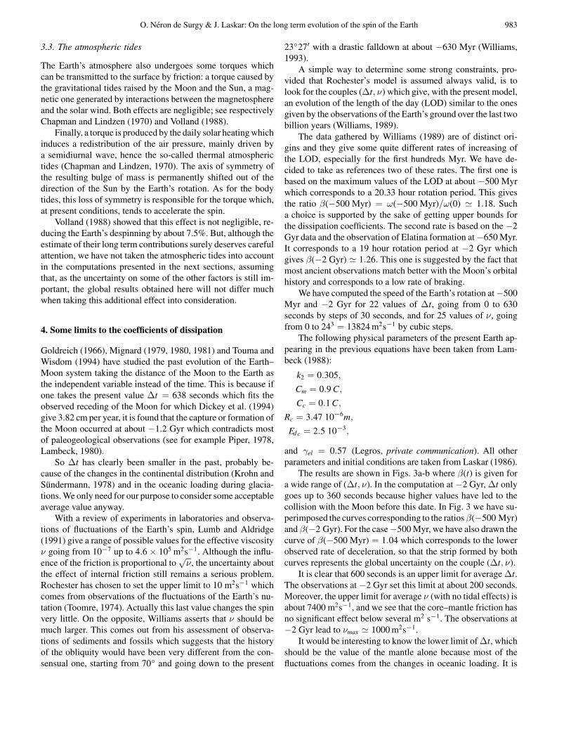
A simple way to determine some strong constraints, pro-vided that Rochester’s model is assumed always valid, is tolook for the couples (∆t, ν) which give, with the present model,an evolution of the length of the day (LOD) similar to the onesgiven by the observations of the Earth’s ground over the last twobillion years (Williams, 1989).

The data gathered by Williams (1989) are of distinct ori-gins and they give some quite different rates of increasing ofthe LOD, especially for the first hundreds Myr. We have de-cided to take as references two of these rates. The first one isbased on the maximum values of the LOD at about −500 Myrwhich corresponds to a 20.33 hour rotation period. This givesthe ratio β(−500 Myr) = ω(−500 Myr)/ω(0) ' 1.18. Sucha choice is supported by the sake of getting upper bounds forthe dissipation coefficients. The second rate is based on the −2Gyr data and the observation of Elatina formation at−650 Myr.It corresponds to a 19 hour rotation period at −2 Gyr whichgives β(−2 Gyr) ' 1.26. This one is suggested by the fact thatmost ancient observations match better with the Moon’s orbitalhistory and corresponds to a low rate of braking.

We have computed the speed of the Earth’s rotation at−500Myr and −2 Gyr for 22 values of ∆t, going from 0 to 630seconds by steps of 30 seconds, and for 25 values of ν, goingfrom 0 to 243 = 13824 m2s−1 by cubic steps.

The following physical parameters of the present Earth ap-pearing in the previous equations have been taken from Lam-beck (1988):

k2 = 0.305,

Cm = 0.9 C,

Cc = 0.1 C,

Rc = 3.47 10−6m,

Ed c = 2.5 10−3,

and γel = 0.57 (Legros, private communication). All otherparameters and initial conditions are taken from Laskar (1986).

The results are shown in Figs. 3a-b where β(t) is given fora wide range of (∆t, ν). In the computation at −2 Gyr, ∆t onlygoes up to 360 seconds because higher values have led to thecollision with the Moon before this date. In Fig. 3 we have su-perimposed the curves corresponding to the ratiosβ(−500 Myr)and β(−2 Gyr). For the case−500 Myr, we have also drawn thecurve of β(−500 Myr) = 1.04 which corresponds to the lowerobserved rate of deceleration, so that the strip formed by bothcurves represents the global uncertainty on the couple (∆t, ν).

It is clear that 600 seconds is an upper limit for average ∆t.The observations at −2 Gyr set this limit at about 200 seconds.Moreover, the upper limit for average ν (with no tidal effects) isabout 7400 m2s−1, and we see that the core–mantle friction hasno significant effect below several m2 s−1. The observations at−2 Gyr lead to νmax ' 1000 m2s−1.

It would be interesting to know the lower limit of ∆t, whichshould be the value of the mantle alone because most of thefluctuations comes from the changes in oceanic loading. It is


Fig. 3. a Percentage of the ratio of the speed of rotation at −500 Myrover the present one for various values of the tidal delay ∆t and the vis-cosity ν. The two bold lines delimit an acceptable range, in agreementwith the observations from sediments and fossils. b Same percentage at−2 000 Myr. The bold line corresponds to the observation of Williams(1989).

possible to give an rough estimate to it, knowing that the energydissipated in the oceans accounts for about 90 or 95% of the total(Zschau, 1978), (Cazenave, 1983), (Mignard, 1983), (Lambeck,1988). In this case, the lowest ∆t would equal 30 or 60 seconds,hence a largest ν of about 600 or 800 m2s−1 if one relies onthe−2 Gyr observations, and about 4400 or 4700 m2s−1 for the−500 Myr ones.

5. Williams’ scenario for the history of the Earth’s obliquity

The dissipation mechanisms presented therein give us someconstraints on scenarios of the Earth’s evolution, and our aimhere would be to provide a general framework in which allscenario for the evolutions of the Earth’s obliquity should bedescribed. As an example, we show here that the dynamicalconstraints obtained here allow to question the scenario pro-posed by Williams (1993). Interpreting observations of variousdeposits in the Earth’s soil which depend on weathering con-

Fig. 4a. Example of possible evolution of the Earth’s obliquity for 5Gyr in the future, for ∆t = 600 s. The background of the figure isthe same one as in Fig. 1, and is a global view of the stability of theobliquity, obtained by means of frequency map analysis (see Laskar andRobutel, 1993). The precession constant (on the left) is plotted againstthe obliquity: the two bold curves correspond to the minimum andmaximum values reached by the obliquity. The right y-axis gives thecorresponding time for the motion. The non-hatched zone correspondsto very regular regions, and we actually observe that in these regions,the motion suffers only small (and regular) variations. The hatchedparts are the regions of strong chaotic behavior. Indeed, in the presentsimulation, as soon as the orbit enters this chaotic zone, very strongvariations of the obliquity are observed, and very high values, close to90 degrees, are reached.

Fig. 4b. Same as Fig. 4a, but with a difference of 10−8 degree in theinitial obliquity.

ditions, Williams devised the following scenario for the pastevolution of the Earth’s obliquity:

a) a slow and regular decreasing from 70 to 60 between−4.5 Gyr and −630 Myr;


b) a quick falldown from 60 to 26 between −630 and−220 Myr;

c) a slow decreasing till the present value.

Concerning the first stage, the main objection to such asmooth evolution arises from the fact that a 70 obliquity wouldimply a crossing of the chaotic zone (see Fig. 1), hence strongfluctuations ranging from about 65 degrees to about 90 degrees(Laskar et al., 1993b).

Then, we have estimated the value of ν which would corre-spond to the second and third ones. The slow decreasing of 2.5

during the last 430 Myr might be possible, the correspondingν being about 300 m2s−1. Now, a falldown from 60 to 26

within 220 Myr gives, with ∆t = 200 seconds, a huge value of1.3 × 106 m2s−1 which exceeds the upper limit of Lumb andAldridge (1991). Such a viscosity would strongly slow downthe Earth and the corresponding LOD in the past would be veryfar from the observed one with β(−220 Myr) ' 1.72.

More simply and independently of the problem of the pos-sible evolution of the value of ν, it is straightforward to verifythat the variations proposed by Williams do not respect relation(R). Indeed, as

cos(26)cos(60)

' 1.8,

we should haveω(−630Myr) = ω(−220Myr)×1.8 which doesnot correspond to any plausible despinning factor even duringthe whole last Gyr.

Williams found a support to his assessment in the very largerate of dε/dt = −0.1′′cy−1 (Kakuta and Aoki, 1972) due tocore–mantle coupling. One one hand, as Rochester (1976) no-ticed it, this value was based on a model which is irrelevant sinceit does not take into account the inertial coupling; Aoki’s model(Aoki, 1969) is adapted only to a slow–rotating planet like Venusat present time for which dω/dt is proportional to ν−1/2 (if νis not too small). On the other hand, Aoki’s model also verifiesrelation (R) — which does not depend on Rochester’s approx-imations —, and such a rate for dε/dt does not correspond tothe low rate of braking ω/ω = −5.8×10−14 proposed by Aokiand Kakuta (1971); Williams thought this last rate was coherentwith the loss of rotational kinetic energy due to CMF estimatedby Rochester, but he did not take the right term of this loss tocompare with.

Williams mentions that some “special conditions” shouldhave occurred at the CMB in order to explain the drastic fall-down. He also suggests that a resonance between the free corenutation and the retrograde annual nutation caused by the so-lar torque may have played an important role. Climate friction(Bills, 1995) might also be a candidate for additional variationsof the obliquity. Such effects remain uncertain. Characteristicsof the Earth’s interior may have been somewhat different in aremote past, but unless system (S) has been very incomplete forsome time in the last Gyr, his scenario should be rejected.

6. the next five billion years evolution of the Earth–Moonsystem

As we have managed to set up some limitations on the possiblevalues of the tidal dissipation and the viscosity of the outercore, by using the available geological observations of the pastevolution of the Earth, we are now ready to study its future overits expected lifetime, i.e. about 5 Gyr.

6.1. with the present tidal coefficient and no core–mantlefriction

Using Laskar’s theory of the solar system, we simultaneouslyintegrate over 5 Gyr the motion of all the planets (Pluto is nottaken into account) and the angular momenta of the Earth andthe Moon with a 250 yr time step.

The equations for the planetary orbital motion used here arethe averaged equations which were previously used by Laskarfor the demonstration of the chaotic behavior of the solar sys-tem. They include the Newtonian interactions of the 8 majorplanets of the solar system (Pluto is neglected), and relativis-tic and Lunar corrections (Laskar, 1985, 1989, 1990). The nu-merical solution of these averaged equations showed excellentagreement when compared over 4400 years with the numeri-cal ephemeris DE102 (Newhall et al., 1983, Laskar, 1986), andover 3 millions years with the numerical integration performedby Quinn, Tremaine and Duncan (Quinn et al., 1991, Laskaret al., 1992). Similar agreement was observed with subsequentnumerical integration by Sussman and Wisdom (1992).

This system of equations was obtained with dedicated com-puter algebra and contains about 50000 monomial terms of theform αz1z2z3z4z5 (Laskar, 1985). It was first constructed in avery extensive way, containing all terms up to second orderwith respect to the masses, and up to 5th degree in eccentricityand inclination, which led to 153824 terms, and then truncatedto improve the efficiency of the integration, without significantloss of precision (Laskar, 1994). The numerical evaluation ofthis simplified system is very efficient, since fewer than 6000monomials need to be evaluated because of symmetries. Numer-ical integration is carried out using an Adams method (PECE)of order 12 and with a 250-year stepsize. The integration errorwas measured by integrating the equations back and forth over10 Myr. It amounts to 3× 10−13 after 107 years (40 000 steps),and behaves like t1.4. Ignoring the chaotic behavior of the orbits,this would give a numerical error of only 4×10−9 after 10 Gyr.

It is clear that because of the chaotic dynamics with a char-acteristic time of 5 Myr, the orbital solution loses its accuracybeyond 100 Myr. This is not important since we do not look forthe exact solution, but for what happens when the system entersthe chaotic zone; the fact that this zone may not be at the exactlocation has not much importance.

We have chosen to take the near present value of 600 secondsfor ∆t and no core–mantle friction. In order to have a statisticalview of the possible behaviors, the whole system is simultane-ously integrated over 5 Gyr for 500 different initial orientationswith obliquities very close to εJ2000 (23 26′ 21.448′′): 10 ini-


Fig. 5. Probability P for the maximum obliquity εmax to exceed a givenvalue ε for the Earth with ∆t = 600s. This was performed over 500orbits with very close initial conditions followed over 5 Gyr.

tial phases ψ separated by 10−9 rad and 50 initial obliquitiesseparated by 10−8 degree.

Thus we have performed a frequency analysis (see Laskar,1993) on the precession frequency and also plotted the minimumand maximum reached obliquity each 10.26 Myr. The wholecomputation, for such an experiment, took about 13 days on aIBM-RS6000/390.

It is quite obvious that we cannot display all the varioussolutions, and we just selected two examples of the possibleevolution of the Earth (Fig.4a-b) which are representative ofthe whole experiment. The two curves plotted in Figs. 4a and4b have initial obliquities differing by 36 µas. We see that theobliquity enters the chaotic region at about +1.5 Gyr and thatit can go from 0 to values close to 90 as was the case in theconservative framework. When superimposed on Fig. 1, thosegraphs show possible paths of the evolving obliquity throughthe different zones of the global dynamics.

The computed speed of rotation of the Earth after 5 Gyris about 0.42 ωin. Provided that ρc ' 10 kg m−3 (Hinderer etal., 1990) and that ψ(5Gyr) < ψin, one can easily check thatcondition (C) of Sect. 3 has not been violated.

The 500 different paths obtained in this manner allow usto get a fairly good idea of the probability for the obliquity toattain some given threshold once the chaotic zone entered. Forinstance, we have found that 342 maximum obliquities haveexceeded 81 at least once, hence a probability P(ε > 81) =68.4% (see Fig. 5).

6.2. some alternatives

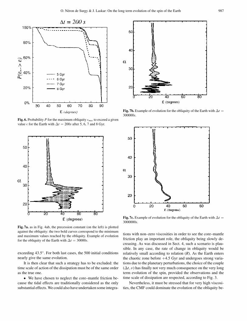
•∆t = 600 seconds is close to the present measured value of thedissipation coefficient, and is in agreement with the observationsat−500 Myr (Fig. 3a), but this leads to a lunar collision at about1.2 Gyr in the past. For this reason, we also considered for ∆tthe smaller value of 200 seconds which is close to the lowestvalue compatible with these geological observations (Fig. 3a).As previously, for ∆t = 200 seconds, we followed the evolutionof 500 obliquities. As the dissipation is three times weaker, theEarth reaches the chaotic zone on a much longer time, after about4.5 Gyr, and after 5 Gyr it has spent only about 500 Myr in thischaotic zone; the probability of reaching a given high value ofobliquity is then lower than in the previous case of ∆t = 600seconds for which the same situation lasted 3.5 Gyr (see Fig.6), and we have P(ε > 81) = 36.6%, which nevertheless isnot a small value. If we continue the integrations over 6 Gyr,which is still a possible future lifetime for the Earth, we obtainfor P(ε > 81) the much higher value of 60.4% (Fig. 6). Wecarried on the computation till 8 Gyr in order to look at theevolution of this probability, and we also plotted in Fig. 6 thecorresponding curves for 7 and 8 Gyr. Then, the set of the fourcurves shows that the longer the Earth remains in the chaoticzone, the higher are the probabilities for the maximum obliquityto reach any value (the possible maximum hardly exceeding 90

after 8 Gyr).

We can thus conclude that for any value of the tidal dis-sipation compatible with the geological observations depictedin Fig. 3a, a very large obliquity in the future of the Earth is ahighly probable event.

Finally, we notice that all curves present a falldown at about70 and a step till a second falldown to 0 close to 90. This can beunderstood by the fact that, as is shown in Laskar et al.(1993b),the chaotic zone is divided into two regions of strong overlapof secular resonances. In each of these regions, the diffusion ofthe orbits is rapid, but the connection between these two boxesis more difficult. As soon as a given orbit enters the second box,related to high values of the obliquity, it will rapidly describeit entirely, so we observe in this case a jump in the maximumvalue reached by the obliquity.

• One would like to consider some very larger coefficients∆t or ν in order to accelerate the effect of the dissipation andto shorten a lot the time of integration by the way. For example,Touma and Wisdom (1994) set a tidal effect about 4000 timesstronger than the present value in their study of the past evolutionof the Earth’s obliquity. We have integrated the system with threedifferent values: ∆t = 3 × 104, 3 × 105, and 3 × 106 seconds,the last one roughly corresponding to what Touma and Wisdomtook. The equivalent despinning of the Earth is then respectivelyachieved after 100 Myr, 10 Myr and 1 Myr instead of 5 Gyr.

The results clearly show that the dynamics are altered asmuch as the time scale of braking is reduced (see Figs. 7a-c). Inthe first case, we have found P(ε > 81) = 1.2%. In the secondone, the obliquity remains confined below 47.3. Finally, secularresonances have a faint effect in the last case, the obliquity never


Fig. 6. Probability P for the maximum obliquity εmax to exceed a givenvalue ε for the Earth with ∆t = 200s after 5, 6, 7 and 8 Gyr.

Fig. 7a. as in Fig. 4ab, the precession constant (on the left) is plottedagainst the obliquity: the two bold curves correspond to the minimumand maximum values reached by the obliquity. Example of evolutionfor the obliquity of the Earth with ∆t = 30000s.

exceeding 43.5. For both last cases, the 500 initial conditionsnearly give the same evolution.

It is then clear that such a strategy has to be excluded: thetime scale of action of the dissipation must be of the same orderas the true one.

• We have chosen to neglect the core–mantle friction be-cause the tidal effects are traditionally considered as the onlysubstantial effects. We could also have undertaken some integra-

Fig. 7b. Example of evolution for the obliquity of the Earth with ∆t =300000s.

Fig. 7c. Example of evolution for the obliquity of the Earth with ∆t =3000000s.

tions with non–zero viscosities in order to see the core–mantlefriction play an important role, the obliquity being slowly de-creasing. As was discussed in Sect. 4, such a scenario is plau-sible. In any case, the rate of change in obliquity would berelatively small according to relation (R). As the Earth entersthe chaotic zone before +4.5 Gyr and undergoes strong varia-tions due to the planetary perturbations, the choice of the couple(∆t, ν) has finally not very much consequence on the very longterm evolution of the spin, provided the observations and thetime scale of dissipation are respected, according to Fig. 3.

Nevertheless, it must be stressed that for very high viscosi-ties, the CMF could dominate the evolution of the obliquity be-


fore the 5 Gyr term. With the highest possible value ν = 7400m2s−1 suggested by the palaeo-observations, dε/dt reaches only−16/Gyr when ω = 0.5ωin. Then, such a situation appears tobe extreme; this supports our studies with ν = 0.

• The formulation of the tidal dissipation used in these in-tegrations corresponds to a model for which the function Q isinversely proportional to the speed of rotation. Consequently, assuggested by MacDonald’s computations (MacDonald, 1964)with a constant geometrical phase lag and the present tidal dis-sipation rate, the choice of the model for which Q is constantwould lead to a faster despinning in the future, and the chaoticzone would be attained sooner.

7. Conclusion

By adding the non-conservative effects to the previous modelfor the long time evolution of the obliquity of the Earth used byLaskar et al., (1993ab), we possess now a complete model forthe study of the long term variations of the spin of the Earth andof the orbit of the Moon over time scales comparable to the ageof the Solar System. It has allowed us to find some significantconstraints on the poorly known tidal time lag ∆t and effectiveviscosity of the outer core ν thanks to paleo–observations, inspite of the uncertainty in the interpretation of geological data.Any further improvement in the knowledge of one of these twoquantities would directly induce an improvement for the secondone and in the history of the Earth’s spin by the way.

It appears in this study that the action of dissipative effectsis weak enough not to cause very significative changes in thebehavior of the obliquity compared to one could expect in aconservative framework, so to say that with a rough idea of thetime scale of these effects, most of the essential dynamics couldbe described from Laskar et al.(1993b), Laskar and Robutel(1993). The combination of this model with Laskar’s seculartheory of the solar system provides us with a powerful tool forexploring plausible scenarii for the long term evolution of theobliquity of the terrestrial planets, and reinforces the importanceof having a global view of the planetary dynamics.

It is still remarkable that in most cases, when using ac-ceptable rates for the dissipation, the obliquity of the Earth ex-plores a large part of the chaotic region discovered by Laskaret al.(1993b), reaching very high maximum values, close to 90degrees.

The chaotic behavior of the obliquity of the Earth preventedus to describe precisely the evolution of its spin over its age,but here we have shown in a simple probabilistic manner thatthe most probable destiny of the Earth is to undergo very strongvariations of its obliquity before the inflation of the Sun, if itdoes not occur.

These computations also confirms that in absence of theMoon, that is for precession constants of the order of 20 arc-sec/year, the Earth would suffer very large variations of its obliq-uity, which could reach nearly 90 degrees with a high probabil-ity.

Finally, it should be noted that the chaotic regions for theobliquity of Venus (Laskar and Robutel, 1993) is very simi-

lar to the one of the Earth (Fig. 1), and thus similar behaviorprobably occurred for this planet in the past. We are presentlyundertaking similar computations for this planet, for which asupplementary difficulty consist in a precise understanding ofthe possible strong effect of the atmospheric tides.

Acknowledgements. We wish to thank Marianne Greff–Lefftz, HilaireLegros, Jacques Hinderer (EOPGS, Strasbourg), Dominique Jault,Jean-Louis Le Mouel and Gautier Hulot (IPG, Paris) for their ex-pressed interest in this work and their help for the understanding ofthe geophysical aspects of this study. The help provided by FredericJoutel concerning some computational aspects of this work was alsovery appreciated. This work was supported by the CEE contract ER-BCHRXCT940460, and by the PNP of CNRS. Part of the computationswere made at CNUSC.

References

Aoki, S.: 1969, AJ, 74, (284-291)Aoki, S., Kakuta, C.: 1971, Cel. Mech., 4, (171-181)Brouwer, D., Clemence, G.M.: 1961, Celestial Mechanics, Academic

PressCazenave, A.: 1983, Tidal friction and the Earth’s rotation, Brosche

and Sundermann, eds., Springer, II, (4-18)Chapman, S., Lindzen, R.S.: 1970, Atmospheric tides (D. Reidel, Dor-

drecht)Darwin, G.H.: 1880, Philos. Trans. R. Soc. London, 171, (713-891)Dickey et al.: 1994, Science, 265, (182-190)Dobrovolskis, A.R.: 1980, Icarus, 41, (18-35)Gold, T., Soter S.: 1969, Icarus, 11, (356-366)Goldreich, P.: 1966, Rev. of Geophys., 4, (411-439)Goldreich, P., Peale S.: 1966, Astron. J., 71, (425-438)Goldreich, P., Peale S.: 1967, AJ, 72, (662-668)Goldreich, P., Peale S.: 1970, AJ, 75, (273-284)Goldreich, P., Soter S.: 1969, Icarus, 5, (375-389)Greenspan, H.P., Howard, L.N.: 1963, J. Fluid Mech., 17, (385).Hide, R.: 1976, Nature, 222, (1055-1056)Hinderer, J.: 1987, These de Doctorat d’Etat, Universite Louis Pasteur

de StrasbourgHinderer, J., Legros, H., Jault, D., Le Mouel, J.-L.: 1990, Physics of

the Earth and Planetary Interiors, 59, (329-341)Kakuta, C., Aoki, S.: 1972, Proceedings of the IAU Symposium No.48,

Reidel, DordrechtKaula, W.: 1964, J. Geophys. Res., 2, (661-685)Kinoshita, H.: 1977, Cel. Mech., 15, (277-326)Kovalevsky, J.: 1963, Introduction a la Mecanique celeste, Armand

Colin, ParisKrohn, J., Sundermann, J.: 1978, Tidal friction and the Earth’s rotation,

Brosche and Sundermann, eds. Springer, I, (190-209)Lago, B., Cazenave A.: 1979, The Moon and the Planets, 21, (127-154)Lambeck, K.: 1979, J. Geophys. Res., 84-B10, (5651-5658)Lambeck, K.: 1980, The Earth’s variable rotation, Cambridge Univer-

sity PressLambeck, K.: 1988, Geophysical Geodesy, Oxford University PressLaskar, J.: 1985, A&A 144, 133Laskar, J.: 1986, A&A, 157, (59-70)Laskar, J.: 1988, Icarus, 88, (266-291)Laskar, J.: 1989, Nature 338, 237Laskar, J.: 1990, Icarus 88, 266Laskar, J., Quinn, T., Tremaine, S.: 1992, Icarus 95, 148


Laskar, J., Joutel, F., Boudin, F.: 1993a, A&A, 270, (522-533)Laskar, J., Joutel, F., Robutel, P.: 1993b, Nature, 361, (615-617)Laskar, J., Robutel, P.: 1993, Nature, 361, (608-612)Laskar, J.: 1993, Physica D, 67, (257-281)Laskar, J.: 1994a, A&A, 287, (L9-L12)Laskar, J.: 1994b, Description des routines utilisateur de TRIP 0.8,

preprintLumb, L.I., Aldridge, K.D.: 1991, J. Geophys. Geoelectr., 43, (93-110)MacDonald G.J.F.: 1964, J. Geophys. Res., 2, (467-541)Marsden, B.G., Cameron, A.G.W.: 1966, The Earth–Moon system

(Plenum Press, N.Y)Mignard, F.: 1979, The Moon and the Planets, 20, (301-315)Mignard, F.: 1980, The Moon and the Planets, 23, (185-206)Mignard, F.: 1981, The Moon and the Planets, 24, (189-207)Mignard, F.: 1983, Tidal friction and the Earth’s rotation, Brosche and

Sundermann, eds. Springer, II, (66-91)Munk, W.H., MacDonald, G.J.: 1960, The rotation of the Earth (Cam-

bridge University Press, N.Y)Newhall, X. X., Standish, E. M., Williams, J. G.: 1983, A&A 125, 150Peale, S.: 1969, AJ, 74, (483-489)Peale, S.: 1974, AJ, 79, (722-744)Peale, S.: 1976, Icarus, 28, (459-467)Piper, J.D.A.: 1978, Tidal friction and the Earth’s rotation, Brosche and

Sundermann, eds. Springer, I, (197-239)

Poincare, H.: 1910, Bull. Astron., 27, (321)Quinn, T.R., Tremaine, S., Duncan, M.: 1991, AJ 101, 2287Rochester, M.G.: 1976, Geophys.J.R.A.S., 46, (109-126)Rubincam, D.P.: 1995, Paleoceanography, 10, (365-372)Smart, W.M.: 1953, Celestial Mechanics (Longmans)Sussman, G.J., and Wisdom, J.: 1992, Sci 257, 56Tisserand, F.: 1891, Traite de Mecanique Celeste (Tome II), (Gauthier–

Villars, Paris)Toomre, A.: 1974, Geophys.J.R.A.S., 38, (335)Touma, J., Wisdom, J.: 1994, AJ, 108, (1943-1961)Volland, H.: 1978, Earth’s rotation from eons to days, Brosche and

Sundermann,eds. Springer, (62-94)Ward, W.R.: 1982, Icarus, 50, (444-448)Ward, W.R.: 1991, Icarus, 94, (160-164)Williams, G.E.: 1989, Episodes, 12, (vol 3)Williams, G.E.: 1993, Earth-Science review, 34, (1-45)Yoder, C.F.: 1995, Icarus, 117, (250-284)Zschau, J.: 1978, Tidal friction and the Earth’s rotation, Brosche and

Sundermann, eds. Springer, I, (62-94)

This article was processed by the author using Springer-Verlag TEXA&A macro package version 4.

on the long term evolution of the spin of the earthaa.springer.de/papers/7318003/2300975.pdf · 976...

Documents