on the log-logistic distribution and its generalizations
TRANSCRIPT
International Journal of Statistics and Probability; Vol. 10, No. 3; May 2021
ISSN 1927-7032 E-ISSN 1927-7040
Published by Canadian Center of Science and Education
93
On the Log-Logistic Distribution and Its Generalizations: A Survey
Abdisalam Hassan Muse1, Samuel M. Mwalili1,2, Oscar Ngesa1,2,3
1 Mathematics Department, Pan African University, Institute of Basic Sciences, Technology, and Innovation, Kenya
2 Statistics and Actuarial Sciences Department, Jomo Kenyatta University of Agriculture and Technology, Kenya
3 Mathematics and Informatics Department, Taita-Taveta University, Kenya
Correspondence: Abdisalam Hassan Muse, Mathematics Department (Statistics Option), Pan African University,
Institute of Basic Sciences, Technology, and Innovation, (PAUSTI), P.O. Box 62000 00200 Nairobi, Kenya.
Received: February 4, 2021 Accepted: April 7, 2021 Online Published: April 20, 2021
doi:10.5539/ijsp.v10n3p93 URL: https://doi.org/10.5539/ijsp.v10n3p93
Abstract
In this paper, we present a review on the log-logistic distribution and some of its recent generalizations. We cite more
than twenty distributions obtained by different generating families of univariate continuous distributions or
compounding methods on the log-logistic distribution. We reviewed some log-logistic mathematical properties,
including the eight different functions used to define lifetime distributions. These results were used to obtain the
properties of some log-logistic generalizations from linear representations. A real-life data application is presented to
compare some of the surveyed distributions.
Keywords: log-logistic distribution, log-logistic generalizations, generalized classes of distributions, construction of
new families, censored data, survival analysis
1. Introduction
The log-logistic distribution, also known as Fisk distribution in economics, is one of the important continuous
probability distributions with a heavy tail defined by one scale (or one rate) and one shape parameters. The log-logistic
distribution is a distribution with a non-negative random variable whose logarithm has the very popular logistic
distribution. It was initially introduced to model population growth by (Verhulst, 1838). It is often applied to model
random lifetimes, and hence has applications in time-to-event analysis. So; if the original data of variable is
𝑥1, 𝑥2, 𝑥3, …, etc., then 𝑙𝑜𝑔 (𝑥1), 𝑙𝑜𝑔(𝑥2), 𝑙𝑜𝑔(𝑥3), …, etc. follow logistic distribution. A logarithmic transformation
on the logistic. The LL distribution is similar in shape to the 2-parameter log-normal distribution but it is more suitable
for use in the time-to-event data analysis since it has heavier tails than the 2-parameter log-normal. The good thing for
log-logistic distribution is that it has greater mathematical tractability when dealing with incomplete (or censored) data
and also its cumulative distribution can be written in closed form. Log-logistic distribution is particularly applicable to
model heavy tailed data in business, medicine, economics, income, wealth, and social sciences. It can also be found in
modeling non-monotone (i.e., unimodal) hazard functions.
The log-logistic distribution has various important properties compared to many other parametric distributions used in
the field of survival and reliability analysis: (i) it is cumulative distribution function (cdf) has an explicit closed-from
expression, which is very useful for analyzing time-to-event data with incomplete information (e.g. censoring and
truncation); (ii) it has a similar shape of pdf and hazard function as the log-normal distribution but has heavier-tails and
the tail properties are what the inference is based on; (iii) it has a non-monotonic hazard function: the hazard function is
unimodal when shape parameter is greater than 1 and is decreasing monotonically when shape parameter is less than or
equal to 1; this is what makes to be different from the Weibull distribution; (iv) it has the potential for analysis of
time-to-event data whose rate increases initially and decreases later; (v) it is also used to analyse the skewed data; (vi)
the LL distribution can be adopted as the basis of an accelerated failure time (AFT) model by allowing the scale
parameter α to differ between groups (Reath et al. 2018), (vii) it has also closed under the proportional odds model;
and the last but not the least (viii) The generalization of the LL distribution has an attractive feature of being a member
to both AFT and Proportional hazard (PH) models. These important properties are what makes that the log-logistic
distribution can be viewed as a simple while useful parametric model which can be widely used in many different
disciplines, including demography for modeling population growth (Verhulst, 1838); economics for the distribution of
wealth or income inequality (Fisk, 1961); engineering for reliability analysis (Ashkar & Mahdi, 2003); and hydrology
for modelling stream flow rates and precipitation (Rowinski et al. 2002) and many other fields.
http://ijsp.ccsenet.org International Journal of Statistics and Probability Vol. 10, No. 3; 2021
94
Some other authors who discussed and studied the properties and applications of LL distribution are (Kleiber and Kotz,
2003) studied the application of LL distribution in economics. Collatt (2003) discussed the application of LL
distribution in health science for modeling the time following for heart transplantation, Tahir et al (2014) discussed it is
useful for modeling censored data usually common in survival and reliability experiments. Other authors who studied
the applications of LL distribution are (Prentice, 1976) (Prentice and Kalbfleisch, 1979); (Bennett, 1983); (Singh and
George, 1988); (Nandram, 1989); (Diekmann, 1992); (Bacon, 1993); (Little et al. 1994); (BRÜEDERL and Diekmann,
1995); (Gupta et al. 1999) among others. The LL distribution has been widely used in different fields such as actuarial
science, economics, survival analysis, reliability analysis, hydrology and engineering. In some cases, the log-logistic
distribution is verified to be a good alternative to the log-normal distribution for modeling censored data in survival and
reliability analysis due to its mathematical simplicity and it is characterizing increasing hazard rate function. However
due to the symmetry of the log-logistic model, it may be poor when the hazard rate is heavily tailed or skewed.
Therefore, there is an increasing trend in generalization of the baseline LL distribution by adding an extra shape
parameter to the parent (or baseline) distribution or by using other generalization techniques. In the statistical literature,
proposing new probability distributions is rich and growing rapidly and various are the papers extending the LL
distribution designed to serve as statistical models for a wide range of real lifetime applications with does not follow
any of the existing probability distributions.
The remainder of the paper is organized as follows. Section 2 reviews the LL distribution, and the two common
parametrization methods for LL distribution and some mathematical properties of the LL distribution are discussed.
Section 3 discussed the extensions of the LL distribution. Section 4 methods for generating new families of continuous
probability distributions and we cite telegraphically twenty distributions obtained by different generated families and
compounding methods on the log-logistic distribution. Section 5 presents the estimation of the parameters. A real-life
data application is presented in section 6. Section 7 we discussed the censored data and the G- families of the
distributions. concluding remarks and the summary of the work is presented in section 8. Finally, Section 9 we highlight
some future works after the survey.
2. Log-logistic Distribution
There are several different parametrizations of the distribution in use. In this study we focused on the two common ones;
scale parametrization and rate parametrization. There are several functions related to continuous probability
distributions. In this study, we focused on those functions which are related to lifetime distributions as a random
variable. The most common ones are; cumulative distribution function (cdf), probability density function (pdf), survival
(reliability function), hazard (failure) rate function (HR), cumulative hazard rate (CHR) function, cumulative hazard
rate average function (HRA), and the conditional survival function (CSF). The good thing for these functions is that
they completely describe the distribution of lifetime, and if you know any of these functions, it is easy to determine the
others.
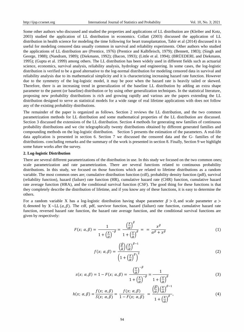
For a random variable X has a log-logistic distribution having shape parameter 𝛽 > 0, and scale parameter 𝛼 >0, denoted by X ~LL (𝛼, 𝛽). The cdf, pdf, survivor function, hazard (failure) rate function, cumulative hazard rate
function, reversed hazard rate function, the hazard rate average function, and the conditional survival functions are
given by respectively:
𝐹(𝑥; 𝛼, 𝛽) = 1
1 + (𝑥𝛼)−𝛽=
(𝑥𝛼)𝛽
1 + (𝑥𝛼)𝛽 = =
𝑥𝛽
𝛼𝛽 + 𝑥𝛽 (1)
𝑓(𝑥; 𝛼, 𝛽) = (𝛽𝛼) (𝑥𝛼)𝛽−1
(1 + (𝑥𝛼)𝛽
)2 (2)
𝑠(𝑥; 𝛼, 𝛽) = 1 − 𝐹(𝑥; 𝛼, 𝛽) = (𝑥𝛼)−𝛽
1 + (𝑥𝛼)−𝛽=
1
1 + (𝑥𝛼)𝛽 (3)
ℎ(𝑥; 𝛼, 𝛽) =𝑓(𝑥; 𝛼, 𝛽)
𝑆(𝑥; 𝛼, 𝛽)=
𝑓(𝑥; 𝛼, 𝛽)
1 − 𝐹(𝑥; 𝛼, 𝛽) =
(𝛽𝛼) (𝑥𝛼)𝛽−1
1 + (𝑥𝛼)𝛽, (4)
http://ijsp.ccsenet.org International Journal of Statistics and Probability Vol. 10, No. 3; 2021
95
𝐻(𝑥) = −𝑙𝑜𝑔𝑅(𝑥) = ∫ ℎ(𝑥)𝑑𝑥, (5) 𝑥
0
𝑟(𝑥; 𝛼, 𝛽) =𝑓(𝑥; 𝛼, 𝛽)
𝐹(𝑥; 𝛼, 𝛽)==
[ (𝛽𝛼) (𝑥𝛼)𝛽−1
(1 + (𝑥𝛼)𝛽
)2
]
[(𝑥𝛼)𝛽
1 + (𝑥𝛼)𝛽 ]
=(𝛽𝛼) (𝑥𝛼)−1
1 + (𝑥𝛼)𝛽 (6)
𝐻𝑅𝐴(𝑥) = 𝐻(𝑥)
𝑥=∫ ℎ(𝑥)𝑑𝑥.𝑥
0
𝑥, 𝑥 > 0, (7)
𝐶𝑆𝐹 = 𝑃(𝑋 > 𝑥 + 𝑡|𝑋 > 𝑡) = 𝑅(𝑥|𝑡) =𝑅(𝑥 + 𝑡)
𝑅(𝑥), 𝑡 > 0, 𝑥 > 0 𝑅(. ) > 0, (8)
Where 𝐹(𝑥; 𝛼, 𝛽)is the CDF of x analogous to H(x) in HRA(x).
2.1 Alternative Parametrization
An alternative parametrization is given by applying the rate parameter which is commonly used in some families like
the exponential distribution (is the reciprocal of the scale parameter α) 𝜌 =1
𝛼
Therefore, without loss of generality the cumulative density function, probability density function, survivor function
and hazard function of the LL distribution are, respectively
𝐹(𝑥) = 1
1 + (𝜌𝑥)−𝛽, (9)
𝑓(𝑥) = 𝛽𝜌(𝜌𝑥)𝛽−1
(1 + (𝜌𝑥)𝛽)2, (10)
𝑆(𝑥) = 1
1 + (𝜌𝑥)𝛽, (11)
ℎ(𝑥) = 𝛽𝜌(𝜌𝑥)𝛽−1
1 + (𝜌𝑥)𝛽, (12)
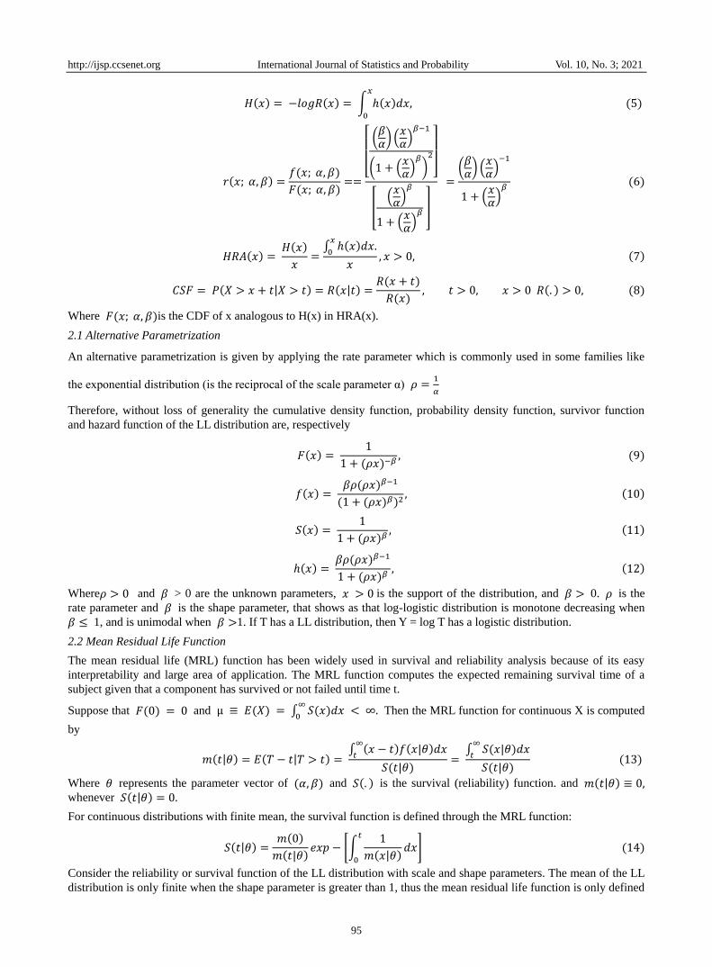
Where𝜌 > 0 and 𝛽 > 0 are the unknown parameters, 𝑥 > 0 is the support of the distribution, and 𝛽 > 0. 𝜌 is the
rate parameter and 𝛽 is the shape parameter, that shows as that log-logistic distribution is monotone decreasing when
𝛽 ≤ 1, and is unimodal when 𝛽 >1. If T has a LL distribution, then Y = log T has a logistic distribution.
2.2 Mean Residual Life Function
The mean residual life (MRL) function has been widely used in survival and reliability analysis because of its easy
interpretability and large area of application. The MRL function computes the expected remaining survival time of a
subject given that a component has survived or not failed until time t.
Suppose that 𝐹(0) = 0 and µ ≡ 𝐸(𝑋) = ∫ 𝑆(𝑥)𝑑𝑥∞
0 < ∞. Then the MRL function for continuous X is computed
by
𝑚(𝑡|𝜃) = 𝐸(𝑇 − 𝑡|𝑇 > 𝑡) = ∫ (𝑥 − 𝑡)𝑓(𝑥|𝜃)𝑑𝑥∞
𝑡
𝑆(𝑡|𝜃)= ∫ 𝑆(𝑥|𝜃)𝑑𝑥∞
𝑡
𝑆(𝑡|𝜃) (13)
Where 𝜃 represents the parameter vector of (𝛼, 𝛽) and 𝑆(. ) is the survival (reliability) function. and 𝑚(𝑡|𝜃) ≡ 0, whenever 𝑆(𝑡|𝜃) = 0.
For continuous distributions with finite mean, the survival function is defined through the MRL function:
𝑆(𝑡|𝜃) =𝑚(0)
𝑚(𝑡|𝜃)𝑒𝑥𝑝 − [∫
1
𝑚(𝑥|𝜃)𝑑𝑥
𝑡
0
] (14)
Consider the reliability or survival function of the LL distribution with scale and shape parameters. The mean of the LL
distribution is only finite when the shape parameter is greater than 1, thus the mean residual life function is only defined
http://ijsp.ccsenet.org International Journal of Statistics and Probability Vol. 10, No. 3; 2021
96
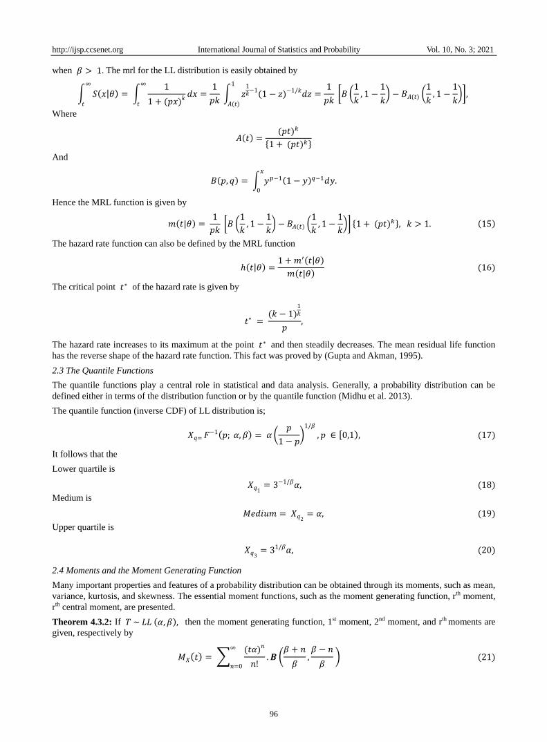
when 𝛽 > 1. The mrl for the LL distribution is easily obtained by
∫ 𝑆(𝑥|𝜃) = ∫1
1 + (𝑝𝑥)𝑘𝑑𝑥 =
1
𝑝𝑘 ∫ 𝑧
1𝑘−1(1 − 𝑧)−1/𝑘𝑑𝑧 =
1
𝑝𝑘 [𝐵 (
1
𝑘, 1 −
1
𝑘) − 𝐵𝐴(𝑡) (
1
𝑘, 1 −
1
𝑘)]
1
𝐴(𝑡)
∞
𝑡
∞
𝑡
,
Where
𝐴(𝑡) =(𝑝𝑡)𝑘
{1 + (𝑝𝑡)𝑘}
And
𝐵(𝑝, 𝑞) = ∫ 𝑦𝑝−1(1 − 𝑦)𝑞−1𝑑𝑦.𝑥
0
Hence the MRL function is given by
𝑚(𝑡|𝜃) = 1
𝑝𝑘 [𝐵 (
1
𝑘, 1 −
1
𝑘) − 𝐵𝐴(𝑡) (
1
𝑘, 1 −
1
𝑘)] {1 + (𝑝𝑡)𝑘}, 𝑘 > 1. (15)
The hazard rate function can also be defined by the MRL function
ℎ(𝑡|𝜃) =1 +𝑚′(𝑡|𝜃)
𝑚(𝑡|𝜃) (16)
The critical point 𝑡∗ of the hazard rate is given by
𝑡∗ = (𝑘 − 1)
1𝑘
𝑝,
The hazard rate increases to its maximum at the point 𝑡∗ and then steadily decreases. The mean residual life function
has the reverse shape of the hazard rate function. This fact was proved by (Gupta and Akman, 1995).
2.3 The Quantile Functions
The quantile functions play a central role in statistical and data analysis. Generally, a probability distribution can be
defined either in terms of the distribution function or by the quantile function (Midhu et al. 2013).
The quantile function (inverse CDF) of LL distribution is;
𝑋𝑞= 𝐹−1(𝑝; 𝛼, 𝛽) = 𝛼 (
𝑝
1 − 𝑝)1/𝛽
, 𝑝 ∈ [0,1), (17)
It follows that the
Lower quartile is
𝑋𝑞1 = 3−1/𝛽𝛼, (18)
Medium is
𝑀𝑒𝑑𝑖𝑢𝑚 = 𝑋𝑞2 = 𝛼, (19)
Upper quartile is
𝑋𝑞3 = 31/𝛽𝛼, (20)
2.4 Moments and the Moment Generating Function
Many important properties and features of a probability distribution can be obtained through its moments, such as mean,
variance, kurtosis, and skewness. The essential moment functions, such as the moment generating function, rth moment,
rth central moment, are presented.
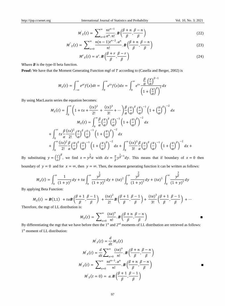
Theorem 4.3.2: If 𝑇 ~ 𝐿𝐿 (𝛼, 𝛽), then the moment generating function, 1st moment, 2nd moment, and rth moments are
given, respectively by
𝑀𝑋(𝑡) = ∑(𝑡𝛼)𝑛
𝑛!
∞
𝑛=0
. 𝑩 (𝛽 + 𝑛
𝛽,𝛽 − 𝑛
𝛽 ) (21)
http://ijsp.ccsenet.org International Journal of Statistics and Probability Vol. 10, No. 3; 2021
97
𝑀′𝑋(𝑡) = ∑
𝑛𝑡𝑛−1
𝛼𝑛. 𝑛!
∞
𝑛=0
. 𝑩 (𝛽 + 𝑛
𝛽,𝛽 − 𝑛
𝛽 ) (22)
𝑀′′𝑋(𝑡) = ∑
𝑛(𝑛 − 1)𝑡𝑛−2. 𝛼𝑛
𝑛!
∞
𝑛=0
. 𝑩 (𝛽 + 𝑛
𝛽,𝛽 − 𝑛
𝛽 ) (23)
𝑀𝑟𝑋(𝑡) = 𝛼𝑟. 𝑩 (
𝛽 + 𝑟
𝛽,𝛽 − 𝑟
𝛽 ) (24)
Where 𝐵 is the type-II beta function.
Proof: We have that the Moment Generating Function mgf of 𝑇 according to (Casella and Berger, 2002) is
𝑀𝑋(𝑡) = ∫ 𝑒𝜌𝑡𝑓(𝑥)𝑑𝑡 = ∫ 𝑒𝑡𝑥𝑓(𝑥)𝑑𝑥 = ∞
0
∞
−∞
∫ 𝑒𝑡𝑥
𝛽𝛼 (𝑥𝛼)𝛽−1
(1 + (𝑥𝛼)𝛽
)2 𝑑𝑥
∞
0
By using MacLaurin series the equation becomes:
𝑀𝑋(𝑡) = ∫ (1 + 𝑡𝑥 +(𝑡𝑥)2
2! +
(𝑡𝑥)3
3!+ ⋯)
𝛽
𝛼(𝑥
𝛼)𝛽
(𝑥
𝛼)−1
(1 + (𝑥
𝛼)𝛽
)−2
𝑑𝑥
∞
0
𝑀𝑋(𝑡) = ∫𝛽
𝛼(𝑥
𝛼)𝛽
(𝑥
𝛼)−1
(1 + (𝑥
𝛼)𝛽
)−2
𝑑𝑥
∞
0
+∫ 𝑡𝑥𝛽
𝛼
(𝑡𝑥)2
2!(𝑥
𝛼)𝛽
(𝑡
𝛼)−1
(1 + (𝑥
𝛼)𝛽
)−2
𝑑𝑥
∞
0
+∫(𝑡𝑥)2
2!
𝛽
𝛼(𝑥
𝛼)𝛽
(𝑥
𝛼)−1
(1 + (𝑥
𝛼)𝛽
)−2
𝑑𝑥 +∫(𝑡𝑥)3
3!
𝛽
𝛼(𝑥
𝛼)𝛽
(𝑥
𝛼)−1
(1 + (𝑥
𝛼)𝛽
)−2
𝑑𝑥 +
∞
0
∞
0
By substituting 𝑦 = (𝑥
𝛼)𝛽
, we find 𝑥 = 𝑦1
𝛽𝛼 with 𝑑𝑥 = 𝛼
𝛽𝑦1
𝛽−1𝑑𝑦. This means that if boundary of 𝑥 = 0 then
boundary of 𝑦 = 0 and for 𝑥 = ∞, then 𝑦 = ∞. Then, the moment generating function it can be written as follows:
𝑀𝑋(𝑡) = ∫1
(1 + 𝑦)2𝑑𝑦 + 𝑡𝛼∫
𝑦1𝛽
(1 + 𝑦)2𝑑𝑦 + (𝑡𝛼)2
∞
0
∫𝑦2𝛽
(1 + 𝑦)2𝑑𝑦
∞
0
+ (𝑡𝛼)3 ∫𝑦3𝛽
(1 + 𝑦)2𝑑𝑦
∞
0
∞
0
By applying Beta Function:
𝑀𝑋(𝑡) = 𝑩(1,1) + 𝑡𝛼𝑩 (𝛽 + 1
𝛽,𝛽 − 1
𝛽 ) +
(𝑡𝛼)2
2!𝑩 (
𝛽 + 1
𝛽,𝛽 − 1
𝛽 ) +
(𝑡𝛼)3
3!(𝛽 + 1
𝛽,𝛽 − 1
𝛽 ) + ⋯
Therefore, the mgt of LL distribution is:
𝑀𝑋(𝑡) = ∑(𝑡𝛼)𝑛
𝑛!
∞
𝑛=0
. 𝑩 (𝛽 + 𝑛
𝛽,𝛽 − 𝑛
𝛽 ) ∎
By differentiating the mgt that we have before then the 1st and 2nd moments of LL distribution are retrieved as follows:
1st moment of LL distribution:
𝑀′𝑋(𝑡) =
𝑑
𝑑𝑡𝑀𝑋(𝑡)
𝑀′𝑋(𝑡) =
𝑑
𝑑𝑡∑
(𝑡𝛼)𝑛
𝑛!
∞
𝑛=0
. 𝑩 (𝛽 + 𝑛
𝛽,𝛽 − 𝑛
𝛽 )
𝑀′𝑋(𝑡) = ∑
𝑛𝑡𝑛−1. 𝛼𝑛
𝑛!
∞
𝑛=0
. 𝑩 (𝛽 + 𝑛
𝛽,𝛽 − 𝑛
𝛽 ) ∎
𝑀′𝑋(𝑡 = 0) = 𝛼. 𝑩 (
𝛽 + 1
𝛽,𝛽 − 1
𝛽 )
http://ijsp.ccsenet.org International Journal of Statistics and Probability Vol. 10, No. 3; 2021
98
2nd moment of LL distribution:
𝑀′′𝑋(𝑡) =
𝑑2
𝑑𝑡2𝑀𝑋(𝑡)
𝑀′′𝑋(𝑡) =
𝑑2
𝑑𝑡2∑
(𝑡𝛼)𝑛
𝑛!
∞
𝑛=0
. 𝑩 (𝛽 + 𝑛
𝛽,𝛽 − 𝑛
𝛽 )
𝑀′′𝑋(𝑡) =∑
𝑛(𝑛 − 1)𝑡𝑛−2. 𝛼𝑛
𝑛!
∞
𝑛=0
. 𝑩 (𝛽 + 𝑛
𝛽,𝛽 − 𝑛
𝛽 ) ∎
𝑀′′𝑋(𝑡 = 0) = 𝛼2. 𝑩 (
𝛽 + 2
𝛽,𝛽 − 2
𝛽 )
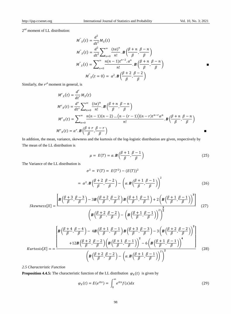
Similarly, the 𝑟𝑡ℎ moment in general, is
𝑀𝑟𝑋(𝑡) =
𝑑𝑟
𝑑𝑡𝑟𝑀𝑋(𝑡)
𝑀𝑟𝑋(𝑡) =
𝑑𝑟
𝑑𝑡𝑟∑
(𝑡𝛼)𝑛
𝑛!
∞
𝑛=0. 𝑩 (
𝛽 + 𝑛
𝛽,𝛽 − 𝑛
𝛽 )
𝑀𝑟𝑋(𝑡) =∑
𝑛(𝑛 − 1)(𝑛 − 2)… (𝑛 − (𝑟 − 1))(𝑛 − 𝑟)𝑡𝑛−𝑟𝛼𝑛
𝑛!
∞
𝑛=0. 𝑩 (
𝛽 + 𝑛
𝛽,𝛽 − 𝑛
𝛽 )
𝑀𝑟𝑋(𝑡) = 𝛼
𝑟 . 𝑩 (𝛽 + 𝑟
𝛽,𝛽 − 𝑟
𝛽 ) ∎
In addition, the mean, variance, skewness and the kurtosis of the log-logistic distribution are given, respectively by
The mean of the LL distribution is
𝜇 = 𝐸(𝑇) = 𝛼.𝑩 (𝛽 + 1
𝛽,𝛽 − 1
𝛽 ) (25)
The Variance of the LL distribution is
𝜎2 = 𝑉(𝑇) = 𝐸(𝑇2) − (𝐸(𝑇))2
= 𝛼2. 𝑩 (𝛽 + 2
𝛽,𝛽 − 2
𝛽 ) − (𝛼. 𝑩 (
𝛽 + 1
𝛽,𝛽 − 1
𝛽 ))
2
(26)
𝑆𝑘𝑒𝑤𝑛𝑒𝑠𝑠[𝑋] =
[𝑩(𝛽 + 3𝛽
,𝛽 − 3𝛽
) − 3𝑩(𝛽 + 2𝛽
,𝛽 − 2𝛽
)𝑩 (𝛽 + 1𝛽
,𝛽 − 1𝛽
) + 2(𝑩(𝛽 + 1𝛽
,𝛽 − 1𝛽
))
𝟑
]
(𝑩(𝛽 + 2𝛽
,𝛽 − 2𝛽
) − (𝑩(𝛽 + 1𝛽
,𝛽 − 1𝛽
))
2
)
𝟑𝟐
(27)
𝐾𝑢𝑟𝑡𝑜𝑠𝑖𝑠[𝑋] = =[ 𝑩 (
𝛽 + 4𝛽
,𝛽 − 4𝛽
) − 4𝑩(𝛽 + 1𝛽
,𝛽 − 1𝛽
)𝑩 (𝛽 + 3𝛽
,𝛽 − 3𝛽
) − 3(𝑩(𝛽 + 2𝛽
,𝛽 − 2𝛽
))
𝟐
+12𝑩(𝛽 + 2𝛽
,𝛽 − 2𝛽
) (𝑩(𝛽 + 1𝛽
,𝛽 − 1𝛽
))
𝟐
− 6(𝑩(𝛽 + 1𝛽
,𝛽 − 1𝛽
))
𝟒
]
(𝑩(𝛽 + 2𝛽
,𝛽 − 2𝛽
) − (𝛼. 𝑩 (𝛽 + 1𝛽
,𝛽 − 1𝛽
))
2
)
𝟐 (28)
2.5 Characteristic Function
Proposition 4.4.5: The characteristic function of the LL distribution 𝜑𝑋(𝑡) is given by
𝜑𝑋(𝑡) = 𝐸(𝑒𝑖𝑡𝑥) = ∫ 𝑒𝑖𝑡𝑥𝑓(𝑥)𝑑𝑥
∞
0
(29)
http://ijsp.ccsenet.org International Journal of Statistics and Probability Vol. 10, No. 3; 2021
99
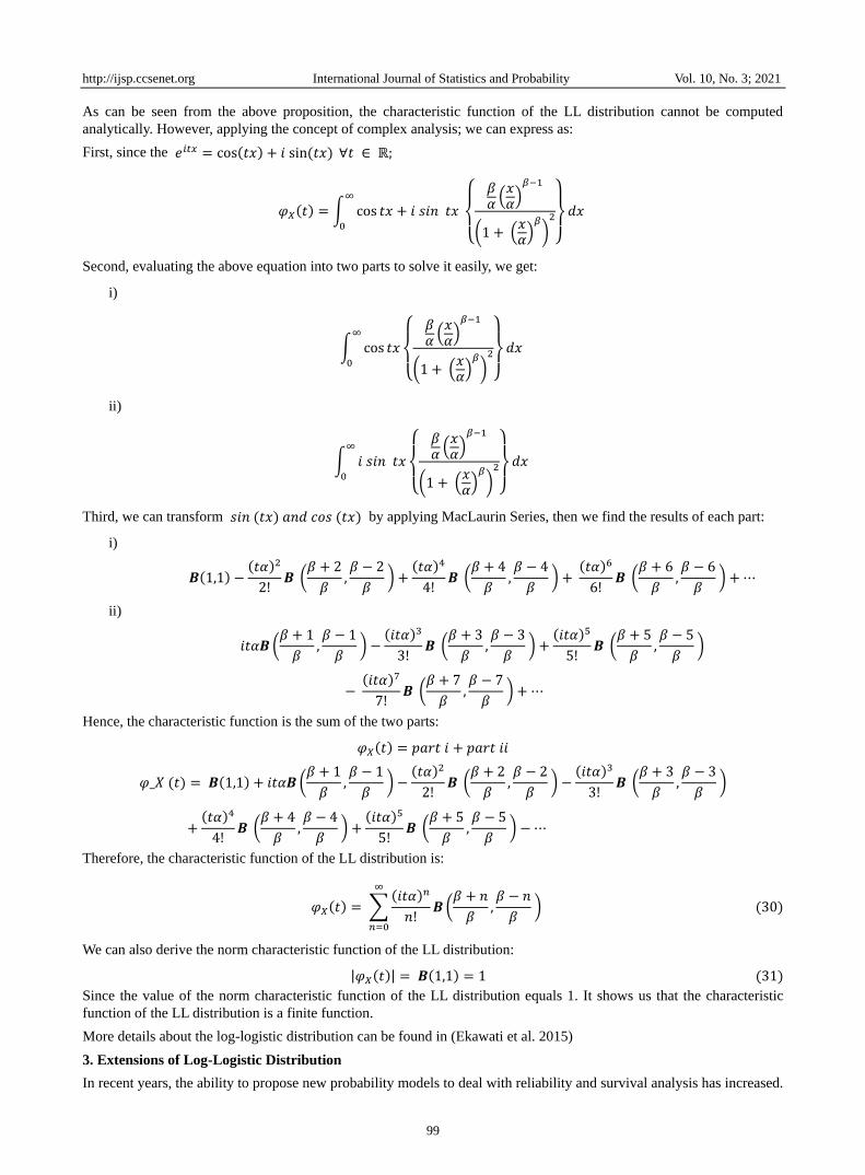
As can be seen from the above proposition, the characteristic function of the LL distribution cannot be computed
analytically. However, applying the concept of complex analysis; we can express as:
First, since the 𝑒𝑖𝑡𝑥 = cos(𝑡𝑥) + 𝑖 sin (𝑡𝑥) ∀𝑡 ∈ ℝ;
𝜑𝑋(𝑡) = ∫ cos 𝑡𝑥 + 𝑖 𝑠𝑖𝑛 𝑡𝑥
{
𝛽𝛼(𝑥𝛼)𝛽−1
(1 + (𝑥𝛼)𝛽
)2
}
𝑑𝑥 ∞
0
Second, evaluating the above equation into two parts to solve it easily, we get:
i)
∫ cos 𝑡𝑥
{
𝛽𝛼(𝑥𝛼)𝛽−1
(1 + (𝑥𝛼)𝛽
)2
}
𝑑𝑥 ∞
0
ii)
∫ 𝑖 𝑠𝑖𝑛 𝑡𝑥
{
𝛽𝛼(𝑥𝛼)𝛽−1
(1 + (𝑥𝛼)𝛽
)2
}
𝑑𝑥 ∞
0
Third, we can transform 𝑠𝑖𝑛 (𝑡𝑥) 𝑎𝑛𝑑 𝑐𝑜𝑠 (𝑡𝑥) by applying MacLaurin Series, then we find the results of each part:
i)
𝑩(1,1) −(𝑡𝛼)2
2!𝑩 (
𝛽 + 2
𝛽,𝛽 − 2
𝛽 ) +
(𝑡𝛼)4
4!𝑩 (
𝛽 + 4
𝛽,𝛽 − 4
𝛽 ) +
(𝑡𝛼)6
6!𝑩 (
𝛽 + 6
𝛽,𝛽 − 6
𝛽 ) +⋯
ii)
𝑖𝑡𝛼𝑩(𝛽 + 1
𝛽,𝛽 − 1
𝛽 ) −
(𝑖𝑡𝛼)3
3!𝑩 (
𝛽 + 3
𝛽,𝛽 − 3
𝛽 ) +
(𝑖𝑡𝛼)5
5!𝑩 (
𝛽 + 5
𝛽,𝛽 − 5
𝛽 )
− (𝑖𝑡𝛼)7
7!𝑩 (
𝛽 + 7
𝛽,𝛽 − 7
𝛽 ) + ⋯
Hence, the characteristic function is the sum of the two parts:
𝜑𝑋(𝑡) = 𝑝𝑎𝑟𝑡 𝑖 + 𝑝𝑎𝑟𝑡 𝑖𝑖
𝜑_𝑋 (𝑡) = 𝑩(1,1) + 𝑖𝑡𝛼𝑩(𝛽 + 1
𝛽,𝛽 − 1
𝛽 ) −
(𝑡𝛼)2
2!𝑩 (
𝛽 + 2
𝛽,𝛽 − 2
𝛽 ) −
(𝑖𝑡𝛼)3
3!𝑩 (
𝛽 + 3
𝛽,𝛽 − 3
𝛽 )
+(𝑡𝛼)4
4!𝑩 (
𝛽 + 4
𝛽,𝛽 − 4
𝛽 ) +
(𝑖𝑡𝛼)5
5!𝑩 (
𝛽 + 5
𝛽,𝛽 − 5
𝛽 ) −⋯
Therefore, the characteristic function of the LL distribution is:
𝜑𝑋(𝑡) = ∑(𝑖𝑡𝛼)𝑛
𝑛!𝑩 (
𝛽 + 𝑛
𝛽,𝛽 − 𝑛
𝛽 ) (30)
∞
𝑛=0
We can also derive the norm characteristic function of the LL distribution:
|𝜑𝑋(𝑡)| = 𝑩(1,1) = 1 (31)
Since the value of the norm characteristic function of the LL distribution equals 1. It shows us that the characteristic
function of the LL distribution is a finite function.
More details about the log-logistic distribution can be found in (Ekawati et al. 2015)
3. Extensions of Log-Logistic Distribution
In recent years, the ability to propose new probability models to deal with reliability and survival analysis has increased.
http://ijsp.ccsenet.org International Journal of Statistics and Probability Vol. 10, No. 3; 2021
100
Many extensions (or generalizations) of the log-logistic distribution have been proposed in the last two decades. In
terms of applications, the log-logistic distribution and its generalizations have become the most popular models for
survival and reliability data. Some recent applications have included: modeling for AIDS and Melanoma data (de
Santana, Ortega, Cordeiro, & Silva, 2012); used for minification process (Gui, 2013); modeling breast cancer data
(Ramos et al. 2013); (Tahir et al. 2014); modeling on censored survival data (Lemonte, 2014); modeling time up to first
calving of cows (Louzada & Granzotto, 2016); modeling, inference, and use to a polled Tabapua Race Time up to First
Calving Data (Granzotto et al. 2017); modeling positive real data in many areas (Lima & Cordeiro, 2017); analysing a
right-censored data (Shakhatreh, 2018); modeling lung cancer data (Alshangiti, et al. 2016); and modeling of breaking
stress data (Aldahlan, 2020).
Because of the increasing interest in terms of applications and methodology, we feel it is timely that a survey is
provided of the log-logistic distribution and its generalizations. In this study, we provide such a review. We review in
the following sections nearly twenty generalizations. For each generalized one, we try to give expressions for the cdf,
pdf, reliability (or survival) function, the failure (or hazard) rate function, the reversed hazard function, the quantile
function and the cumulative hazard function. Sometimes not all of these functions are given if they are not stated in the
original source or if nice closed form expressions are not known.
In the statistics and probability, the literature on statistical theory abounds in surveys of topics of current interest.
Ghitany (1998) provided thorough reviews of the recent modifications of the gamma distribution. Pham and Lai (2007)
provided through reviews of the recent generalizations of the Weibull distribution. Nadarajah (2013) provided an
extensive survey of the exponentiated Weibull distribution. Li and Nadarajah (2020) provided an extensive review of
the student’s t distribution and its generalizations. Rahman et al. (2020) provided an expository review of the
transmuted probability distributions. Tomy et al. 2020) provided an extensive review of the recent generalizations of the
exponential distribution. Dey, et al. (2021) provided an extensive review of the transmuted distributions. We contribute
to the literature by reviewing the log-logistic distribution and its generalizations. While it is common to come across
reviews which deal with generalizations of an existing distributions, our approach is significantly different. Our focus is
on the method. To be the best of our knowledge, there is no other work which attempts to bring together at one place
nearly twenty generalizations (or extensions) of the LL distribution. In this work, we have reviewed only univariate
log-logistic distribution and related distributions. A future work is to review bivariate, multivariate, matrix variate and
complex variate log-logistic distribution.
4. Review of the Methods for Building New Log-Logistic Distributions
In this section, we present up-to-date review of the methods for building new families of continuous probability
distributions. In probability and applied statisticians have shown great interest in building and generating new
generalized probability models that extend well-known probability distributions and are more flexible for data modeling
in many different disciplines of applications.in recent decades, some different extensions of continuous distributions
have received great attention in the recent literature. Gupta and Kundu (2009) discussed six different techniques for the
induction of shape/skewness parameter(s) in probability distributions namely: (1) method of proportional hazard model,
(2) method of proportional reversed hazard model, (3) method of proportional cumulants model, (4) method of
proportional odds model, (5) method of power transformed model, and (6) method of Azzalini’s skewed model. On the
other hand, Lee et al. (2013), reviewed the different methods of generating new probability distributions and they
focused on the two main techniques; adding parameters and combining existing probability distributions. On the other
hand, they discussed three methods developed before 1980s, and they are: (1) method of differential equation, (2)
method of transformation, and (3) method of quantile. Then they discussed five generating techniques developed since
1980s, those are : (1) method of adding parameters to an existing distribution, (2) composite method, (3) the
beta-generated method, (4) the transformed-transformer (T-X) method, and (5) methods of generating skewed
distributions. Tahir and Nadarajah (2015) wrote a review of methods for generating probability distributions with more
than 300 reference papers, most of these distributions were introduced in the recent years, (Nadarajah et al. 2013);
(Tahir and Cordeiro (2015), (Ahmad et al. 2019) and (De Brito et al. 2019) gives an excellent review on the recent
developments of univariate continuous distributions.
This study work offers a survey of recently different methods for developing families of probability distributions. The
technique of obtaining a new generalized distribution is of different forms; generally speaking, the five methods
developed since 1980s, can be named them as a combination methods because of the reason because of the reason that
these techniques attempt to add an extra parameters to an existing probability distribution or combining existing
distributions into new distributions (Lee et al., 2013). In this work, we will categorize into two headings; (1) generator
method or Parameter Induction method, and (2) Compound method.
http://ijsp.ccsenet.org International Journal of Statistics and Probability Vol. 10, No. 3; 2021
101
4.1 Generator Method
There are several different methods described in the literature used to extend well-known probability distributions.
Probably, one of the most popular method is to consider distribution generators and is called generator method (also
known as parameter induction method). The method deals with an induction a shape parameter(s) to a baseline (or
parent) distribution to improve goodness-of-fits and to explore tail properties. In the generator method, we can
categorize into; exponentiated-G family, beta-G family, gamma-G family, Marshall-Olkin class, Kumaraswamy class,
transmuted family, cubic transmuted family, a general transmuted family, alpha-power transformation, T-X family
method, Zubair-G family, and the Cordeiro-Tahir’s family.
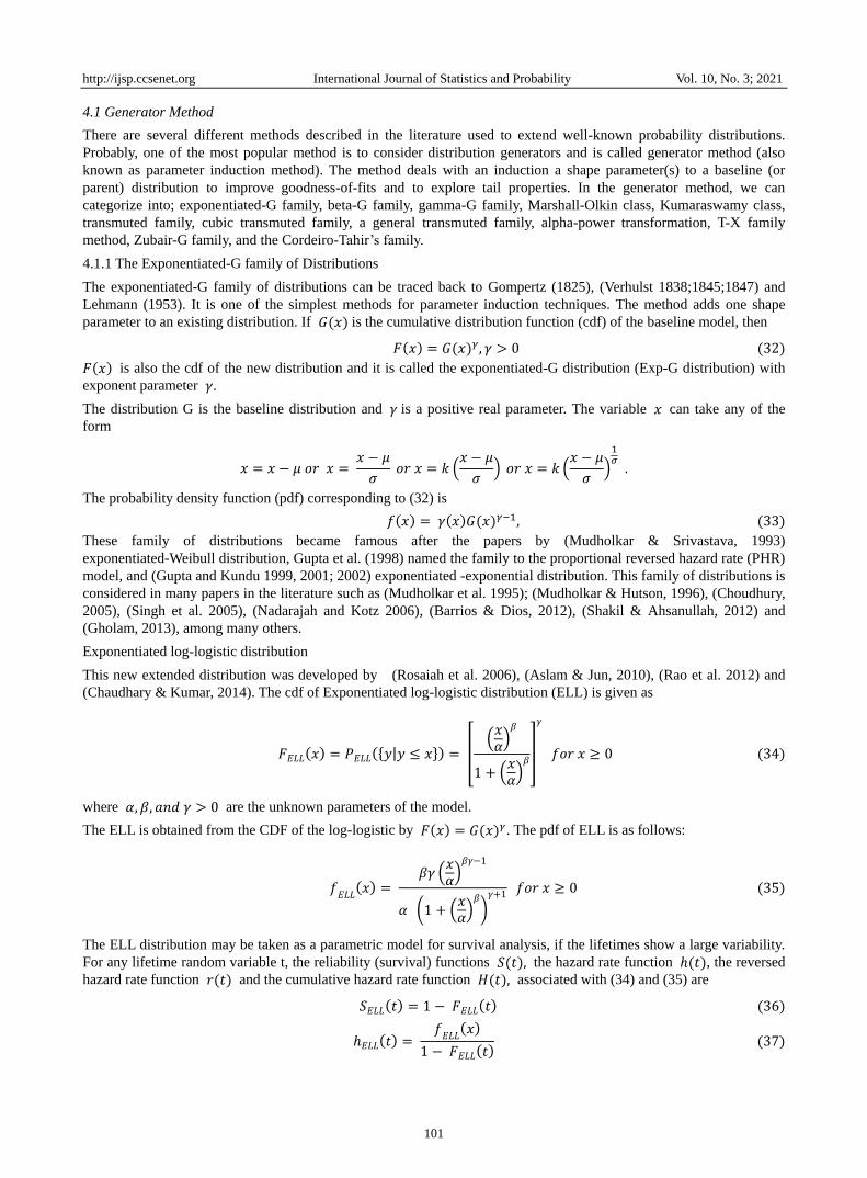
4.1.1 The Exponentiated-G family of Distributions
The exponentiated-G family of distributions can be traced back to Gompertz (1825), (Verhulst 1838;1845;1847) and
Lehmann (1953). It is one of the simplest methods for parameter induction techniques. The method adds one shape
parameter to an existing distribution. If 𝐺(𝑥) is the cumulative distribution function (cdf) of the baseline model, then
𝐹(𝑥) = 𝐺(𝑥)𝛾, 𝛾 > 0 (32)
𝐹(𝑥) is also the cdf of the new distribution and it is called the exponentiated-G distribution (Exp-G distribution) with
exponent parameter 𝛾.
The distribution G is the baseline distribution and 𝛾 is a positive real parameter. The variable 𝑥 can take any of the
form
𝑥 = 𝑥 − 𝜇 𝑜𝑟 𝑥 = 𝑥 − 𝜇
𝜎 𝑜𝑟 𝑥 = 𝑘 (
𝑥 − 𝜇
𝜎) 𝑜𝑟 𝑥 = 𝑘 (
𝑥 − 𝜇
𝜎)
1𝜎 .
The probability density function (pdf) corresponding to (32) is
𝑓(𝑥) = 𝛾(𝑥)𝐺(𝑥)𝛾−1, (33)
These family of distributions became famous after the papers by (Mudholkar & Srivastava, 1993)
exponentiated-Weibull distribution, Gupta et al. (1998) named the family to the proportional reversed hazard rate (PHR)
model, and (Gupta and Kundu 1999, 2001; 2002) exponentiated -exponential distribution. This family of distributions is
considered in many papers in the literature such as (Mudholkar et al. 1995); (Mudholkar & Hutson, 1996), (Choudhury,
2005), (Singh et al. 2005), (Nadarajah and Kotz 2006), (Barrios & Dios, 2012), (Shakil & Ahsanullah, 2012) and
(Gholam, 2013), among many others.
Exponentiated log-logistic distribution
This new extended distribution was developed by (Rosaiah et al. 2006), (Aslam & Jun, 2010), (Rao et al. 2012) and
(Chaudhary & Kumar, 2014). The cdf of Exponentiated log-logistic distribution (ELL) is given as
𝐹𝐸𝐿𝐿(𝑥) = 𝑃𝐸𝐿𝐿({𝑦|𝑦 ≤ 𝑥}) = [(𝑥𝛼)𝛽
1 + (𝑥𝛼)𝛽]
𝛾
𝑓𝑜𝑟 𝑥 ≥ 0 (34)
where 𝛼, 𝛽, 𝑎𝑛𝑑 𝛾 > 0 are the unknown parameters of the model.
The ELL is obtained from the CDF of the log-logistic by 𝐹(𝑥) = 𝐺(𝑥)𝛾. The pdf of ELL is as follows:
𝑓𝐸𝐿𝐿(𝑥) =
𝛽𝛾 (𝑥𝛼)𝛽𝛾−1
𝛼 (1 + (𝑥𝛼)𝛽
)𝛾+1 𝑓𝑜𝑟 𝑥 ≥ 0 (35)
The ELL distribution may be taken as a parametric model for survival analysis, if the lifetimes show a large variability.
For any lifetime random variable t, the reliability (survival) functions 𝑆(𝑡), the hazard rate function ℎ(𝑡), the reversed
hazard rate function 𝑟(𝑡) and the cumulative hazard rate function 𝐻(𝑡), associated with (34) and (35) are
𝑆𝐸𝐿𝐿(𝑡) = 1 − 𝐹𝐸𝐿𝐿(𝑡) (36)
ℎ𝐸𝐿𝐿(𝑡) = 𝑓𝐸𝐿𝐿(𝑥)
1 − 𝐹𝐸𝐿𝐿(𝑡) (37)
http://ijsp.ccsenet.org International Journal of Statistics and Probability Vol. 10, No. 3; 2021
102
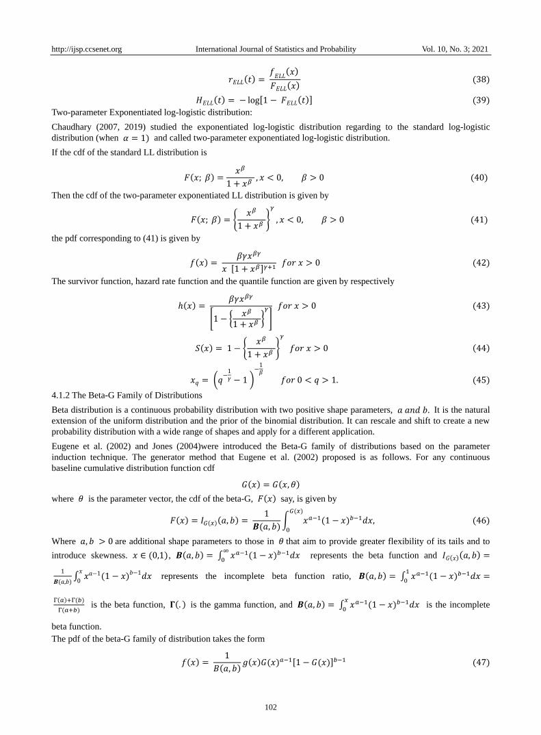
𝑟𝐸𝐿𝐿(𝑡) = 𝑓𝐸𝐿𝐿(𝑥)
𝐹𝐸𝐿𝐿(𝑥) (38)
𝐻𝐸𝐿𝐿(𝑡) = − log[1 − 𝐹𝐸𝐿𝐿(𝑡)] (39)
Two-parameter Exponentiated log-logistic distribution:
Chaudhary (2007, 2019) studied the exponentiated log-logistic distribution regarding to the standard log-logistic
distribution (when 𝛼 = 1) and called two-parameter exponentiated log-logistic distribution.
If the cdf of the standard LL distribution is
𝐹(𝑥; 𝛽) =𝑥𝛽
1 + 𝑥𝛽 , 𝑥 < 0, 𝛽 > 0 (40)
Then the cdf of the two-parameter exponentiated LL distribution is given by
𝐹(𝑥; 𝛽) = {𝑥𝛽
1 + 𝑥𝛽 }
𝛾
, 𝑥 < 0, 𝛽 > 0 (41)
the pdf corresponding to (41) is given by
𝑓(𝑥) = 𝛽𝛾𝑥𝛽𝛾
𝑥 [1 + 𝑥𝛽]𝛾+1 𝑓𝑜𝑟 𝑥 > 0 (42)
The survivor function, hazard rate function and the quantile function are given by respectively
ℎ(𝑥) = 𝛽𝛾𝑥𝛽𝛾
[1 − {𝑥𝛽
1 + 𝑥𝛽 }𝛾
]
𝑓𝑜𝑟 𝑥 > 0 (43)
𝑆(𝑥) = 1 − {𝑥𝛽
1 + 𝑥𝛽 }
𝛾
𝑓𝑜𝑟 𝑥 > 0 (44)
𝑥𝑞 = (𝑞−1𝛾 − 1 )
−1𝛽
𝑓𝑜𝑟 0 < 𝑞 > 1. (45)
4.1.2 The Beta-G Family of Distributions
Beta distribution is a continuous probability distribution with two positive shape parameters, 𝑎 𝑎𝑛𝑑 𝑏. It is the natural
extension of the uniform distribution and the prior of the binomial distribution. It can rescale and shift to create a new
probability distribution with a wide range of shapes and apply for a different application.
Eugene et al. (2002) and Jones (2004)were introduced the Beta-G family of distributions based on the parameter
induction technique. The generator method that Eugene et al. (2002) proposed is as follows. For any continuous
baseline cumulative distribution function cdf
𝐺(𝑥) = 𝐺(𝑥, 𝜃)
where 𝜃 is the parameter vector, the cdf of the beta-G, 𝐹(𝑥) say, is given by
𝐹(𝑥) = 𝐼𝐺(𝑥)(𝑎, 𝑏) = 1
𝑩(𝑎, 𝑏)∫ 𝑥𝑎−1(1 − 𝑥)𝑏−1𝑑𝑥,𝐺(𝑥)
0
(46)
Where 𝑎, 𝑏 > 0 are additional shape parameters to those in 𝜃 that aim to provide greater flexibility of its tails and to
introduce skewness. 𝑥 ∈ (0,1), 𝑩(𝑎, 𝑏) = ∫ 𝑥𝑎−1(1 − 𝑥)𝑏−1𝑑𝑥∞
0 represents the beta function and 𝐼𝐺(𝑥)(𝑎, 𝑏) =
1
𝑩(𝑎,𝑏)∫ 𝑥𝑎−1(1 − 𝑥)𝑏−1𝑑𝑥 𝑥
0 represents the incomplete beta function ratio, 𝑩(𝑎, 𝑏) = ∫ 𝑥𝑎−1(1 − 𝑥)𝑏−1𝑑𝑥 =
1
0
Γ(𝑎)+Γ(𝑏)
Γ(𝑎+𝑏) is the beta function, 𝚪(. ) is the gamma function, and 𝑩(𝑎, 𝑏) = ∫ 𝑥𝑎−1(1 − 𝑥)𝑏−1𝑑𝑥
𝑥
0 is the incomplete
beta function.
The pdf of the beta-G family of distribution takes the form
𝑓(𝑥) = 1
𝐵(𝑎, 𝑏)𝑔(𝑥)𝐺(𝑥)𝑎−1[1 − 𝐺(𝑥)]𝑏−1 (47)
http://ijsp.ccsenet.org International Journal of Statistics and Probability Vol. 10, No. 3; 2021
103
The beta-G family is also called the beta logit family. These family of distributions become much more popular after
Eugene et al. (2002) .This class is studied and discussed the estimation methods and the characterization by maximum
entropy by (Zografos & Balakrishnan, 2009) and the moments from beta-G family are studied by (Cordeiro &
Nadarajah, 2011)
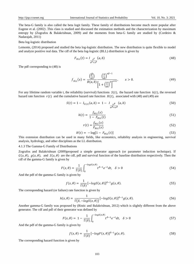
Beta log-logistic distribution
Lemonte, (2014) proposed and studied the beta log-logistic distribution. The new distribution is quite flexible to model
and analyze positive real data. The cdf of the beta log-logistic (BLL) distribution is given by
𝐹𝐵𝐿𝐿(𝑡) = 𝐼 𝑥𝛽
𝛼𝛽+𝑥𝛽
(𝑎, 𝑏) (48)
The pdf corresponding to (48) is
𝑓𝐵𝐿𝐿(𝑥) =
(𝛽𝛼)
𝐵(𝑎, 𝑏)
(𝑥𝛼)𝑎𝛽−1
[1 + (𝑥𝛼)𝛽
]𝑎+𝑏
, 𝑥 > 0. (49)
For any lifetime random variable t, the reliability (survival) functions 𝑆(𝑡), the hazard rate function ℎ(𝑡), the reversed
hazard rate function 𝑟(𝑡) and the cumulative hazard rate function 𝐻(𝑡), associated with (48) and (49) are
𝑆(𝑡) = 1 − 𝐼𝐺(𝑥)(𝑎, 𝑏) = 1 − 𝐼 𝑥𝛽
𝛼𝛽+𝑥𝛽
(𝑎, 𝑏) (50)
ℎ(𝑡) = 𝑓𝐵𝐿𝐿(𝑥)
1 − 𝐹𝐵𝐿𝐿(𝑡) (51)
𝑟(𝑡) =𝑓𝐵𝐿𝐿(𝑥)
𝐹𝐵𝐿𝐿(𝑥) (52)
𝐻(𝑡) = − log[1 − 𝐹𝐵𝐿𝐿(𝑡)] (53)
This extension distribution can be used in many fields, like economics, reliability analysis in engineering, survival
analysis, hydrology, and other disciplines as the LL distribution.
4.1.3 The Gamma-G Family of Distributions
Zografos and Balakrishnan (2009)proposed a simple generator approach (or parameter induction technique). If
𝐺(𝑥, 𝜃), 𝑔(𝑥, 𝜃), and 𝑆(𝑥, 𝜃) are the cdf, pdf and survival function of the baseline distribution respectively. Then the
cdf of the gamma-G family is given by
𝐹(𝑥, 𝜃) = 1
Γ(𝛿)∫ 𝑡𝛿−1𝑒−𝑡𝑑𝑡, 𝛿 > 0 (54)−𝑙𝑜𝑔𝑆(𝑥,𝜃)
0
And the pdf of the gamma-G family is given by
𝑓(𝑥, 𝜃) = 1
Γ(𝛿)[−𝑙𝑜𝑔𝑆(𝑥, 𝜃)]𝛿−1𝑔(𝑥, 𝜃). (55)
The corresponding hazard (or failure) rate function is given by
ℎ(𝑥, 𝜃) = 1
Γ(𝛿, −𝑙𝑜𝑔𝑆(𝑥, 𝜃))[−𝑙𝑜𝑔𝑆(𝑥, 𝜃)]𝛿−1𝑔(𝑥, 𝜃). (56)
Another gamma-G family was proposed by (Ristic and Balakrishnan, 2012) which is slightly different from the above
generator. The cdf and pdf of their generator was defined by
𝐹(𝑥, 𝜃) = 1 − 1
Γ(𝛿)∫ 𝑡𝛿−1𝑒−𝑡𝑑𝑡, 𝛿 > 0 (57)−𝑙𝑜𝑔𝑆(𝑥,𝜃)
0
And the pdf of the gamma-G family is given by
𝑓(𝑥, 𝜃) = 1
Γ(𝛿)[−𝑙𝑜𝑔𝐹(𝑥, 𝜃)]𝛿−1𝑔(𝑥, 𝜃). (58)
The corresponding hazard function is given by
http://ijsp.ccsenet.org International Journal of Statistics and Probability Vol. 10, No. 3; 2021
104
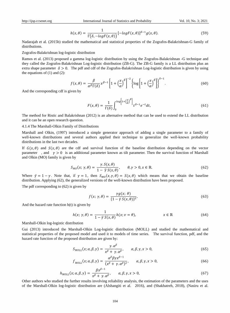
ℎ(𝑥, 𝜃) = 1
Γ(𝛿, −𝑙𝑜𝑔𝐹(𝑥, 𝜃))[−𝑙𝑜𝑔𝐹(𝑥, 𝜃)]𝛿−1𝑔(𝑥, 𝜃). (59)
Nadarajah et al. (2015b) studied the mathematical and statistical properties of the Zografos-Balakrishnan-G family of
distributions.
Zografos-Balakrishnan log-logistic distribution
Ramos et al. (2013) proposed a gamma log-logistic distribution by using the Zografos-Balakrishnan -G technique and
they called the Zografos-Balakrishnan Log-logistic distribution (ZB-G). The ZB-G family is a LL distribution plus an
extra shape parameter 𝛿 > 0. The pdf and cdf of the Zografos-Balakrishnan Log-logistic distribution is given by using
the equations of (1) and (2):
𝑓(𝑥, 𝜃) = 𝛽
𝛼𝛽Γ(𝛿)𝑥𝛽−1 [1 + (
𝑥
𝛼)𝛽
]
−2
{log [1 + (𝑥
𝛼)𝛽
]}
𝛿−1
. (60)
And the corresponding cdf is given by
𝐹(𝑥, 𝜃) = 1
Γ(𝛿)∫ 𝑡𝛿−1𝑒−𝑡𝑑𝑡, (61)𝑙𝑜𝑔[1+(
𝑥𝛼)
𝛽]
0
The method for Ristic and Balakrishnan (2012) is an alternative method that can be used to extend the LL distribution
and it can be an open research question.
4.1.4 The Marshall-Olkin Family of Distributions
Marshall and Olkin, (1997) introduced a simple generator approach of adding a single parameter to a family of
well-known distributions and several authors applied their technique to generalize the well-known probability
distributions in the last two decades.
If 𝐺(𝑥, 𝜃) and 𝑆(𝑥, 𝜃) are the cdf and survival function of the baseline distribution depending on the vector
parameter , and 𝛾 > 0 is an additional parameter known as tilt parameter. Then the survival function of Marshall
and Olkin (MO) family is given by
𝑆𝑀𝑂(𝑥; 𝛾, 𝜃) = 𝛾. 𝑆(𝑥, 𝜃)
1 − �̅� 𝑆(𝑥, 𝜃), 𝜃, 𝛾 > 0, 𝑥 ∈ ℝ. (62)
Where �̅� = 1 − 𝛾 . Note that, if 𝛾 = 1 , then 𝑆𝑀𝑂(𝑥, 𝛾, 𝜃) = 𝑆(𝑥, 𝜃) which means that we obtain the baseline
distribution. Applying (62), the generalized versions of the well-known distribution have been proposed.
The pdf corresponding to (62) is given by
𝑓(𝑥; 𝛾, 𝜃) = 𝛾𝑔(𝑥; 𝜃)
{1 − �̅� 𝑆(𝑥, 𝜃)}2, (63)
And the hazard rate function h(t) is given by
ℎ(𝑥; 𝛾, 𝜃) = 1
1 − �̅� 𝑆(𝑥, 𝜃)ℎ(𝑥; 𝑣 = 𝜃), 𝑥 ∈ ℝ (64)
Marshall-Olkin log-logistic distribution
Gui (2013) introduced the Marshall-Olkin Log-logistic distribution (MOLL) and studied the mathematical and
statistical properties of the proposed model and used it to models of time series. The survival function, pdf, and the
hazard rate function of the proposed distribution are given by:
𝑆𝑀𝑂𝐿𝐿(𝑥; 𝛼, 𝛽, 𝛾) = 𝛾. 𝛼𝛽
𝑥𝛽 + 𝛾. 𝛼𝛽, 𝛼, 𝛽, 𝛾, 𝑥 > 0, (65)
𝑓𝑀𝑂𝐿𝐿
(𝑥; 𝛼, 𝛽, 𝛾) = 𝛼𝛽𝛽𝛾𝑥𝛽−1
(𝑥𝛽 + 𝛾. 𝛼𝛽)2, 𝛼, 𝛽, 𝛾, 𝑥 > 0, (66)
ℎ𝑀𝑂𝐿𝐿(𝑥; 𝛼, 𝛽, 𝛾) = 𝛽𝑥𝛽−1
𝑥𝛽 + 𝛾. 𝛼𝛽, 𝛼, 𝛽, 𝛾, 𝑥 > 0, (67)
Other authors who studied the further results involving reliability analysis, the estimation of the parameters and the uses
of the Marshall-Olkin log-logistic distribution are (Alshangiti et al. 2016), and (Shakhatreh, 2018), (Nasiru et al.
http://ijsp.ccsenet.org International Journal of Statistics and Probability Vol. 10, No. 3; 2021
105
2019)
4.1.5 The Alpha Power Transformation
Mahdavi and Kundu (2017) proposed a new generator technique that many authors applied to introduce for new
statistical distributions to increase flexibility of the given family. The technique adds a new parameter to the baseline
distribution. The cdf of Alpha power transformation (AP) is defined as
𝐹𝐴𝑃𝑇(𝑥; 𝜃, 𝛾) = 𝛾𝐺(𝑥;𝜃) − 1
𝛾 − 1
′
𝜃, 𝛾 > 0 , 𝛾 ≠ 1, 𝑥 ∈ ℝ. (68)
where 𝐺(𝑥; 𝜃) is the cdf of the baseline distribution and 𝜃 is the vector parameter.
The pdf corresponding to (68) is given as
𝐹𝐴𝑃𝑇(𝑥; 𝜃, 𝛾) = log(𝛾) 𝛾
𝐺(𝑥;𝜃)
𝛾 − 1𝑔(𝑥; 𝜃); 𝜃, 𝛾 > 0 , 𝛾 ≠ 1, 𝑥 ∈ ℝ. (69)
Two-parameter Alpha Power Transformed Log-logistic distribution
Several researchers have applied the alpha power technique to extend the log-logistic distribution.
Malik and Ahmad (2020) proposed the two-parameter alpha power log-logistic distribution (APLL) of two unknown
parameters 𝜃 scale parameters and 𝛾 shape parameter. Note that, Malik and Ahmad (2020) extended the standard
log-logistic distribution (where the shape parameter equals 1).
If the cdf of the standard LL distribution takes the form:
𝐹(𝑥; 𝜃) = 𝑥𝜃
1 + 𝑥𝜃, (70)
Then the cdf of the APLL is given by
𝐹𝐴𝑃𝐿𝐿(𝑥; 𝜃, 𝛾) = 𝛾 (
𝑥𝜃
1 + 𝑥𝜃 ) − 1
𝛾 − 1 𝜃, 𝛾 > 0 , 𝛾 ≠ 1, 𝑥 ∈ ℝ. (71)
The pdf corresponding to (71) is given by
𝑓𝐴𝑃𝐿𝐿
(𝑥; 𝜃, 𝛾) = log(𝛾)
𝛾 − 1
𝜃𝑥𝜃−1
(1 + 𝑥𝜃)2𝛾(𝑥𝜃
1+𝑥𝜃); 𝜃, 𝛾 > 0 , 𝛾 ≠ 1, 𝑥 ∈ ℝ. (72)
The survival function of the APLL is defined as
𝑆𝐴𝑃𝐿𝐿(𝑥; 𝜃, 𝛾) = 𝛾(𝑥𝜃
1+𝑥𝜃)[𝛾(
1
1+𝑥𝜃 )−1
𝛾−1]
; 𝜃, 𝛾 > 0 , 𝛾 ≠ 1, 𝑥 ∈ ℝ. (73)
The hazard rate function of the APLL is given by
ℎ𝐴𝑃𝐿𝐿(𝑥; 𝜃, 𝛾) = log (𝛾)𝜃𝑥𝜃−1
(1 + 𝑥𝜃)21
𝛾 (1
1 + 𝑥𝜃 ) − 1
; 𝜃, 𝛾 > 0 , 𝛾 ≠ 1, 𝑥 ∈ ℝ. (74)
The reverse hazard rate function of the APLL is given by
𝑟𝐴𝑃𝐿𝐿(𝑥; 𝜃, 𝛾) = log (𝛾)𝜃𝑥𝜃−1
(1 + 𝑥𝜃)2
𝛾 (1
1 + 𝑥𝜃 )
𝛾 (1
1 + 𝑥𝜃 )− 1
; 𝜃, 𝛾 > 0 , 𝛾 ≠ 1, 𝑥 ∈ ℝ. (75)
The Alpha Power Transformed Log-logistic distribution
Aldahlan (2020) proposed an Alpha Power Transformed Log-logistic distribution (APTLL) and studied the
mathematical and statistical properties of the new distribution. Aldahlan (2020) extended the two-parameter
log-logistic distribution. If the cdf of the two-parameter baseline log-logistic distribution takes the form:
𝐹(𝑥; 𝛼, 𝛽) = 1
1 + (𝑥𝛼)−𝛽, (76)
http://ijsp.ccsenet.org International Journal of Statistics and Probability Vol. 10, No. 3; 2021
106
Then the cdf of the APTLL is given by
𝐹𝐴𝑃𝑇𝐿𝐿(𝑥; 𝛼, 𝛽, 𝛾) =
𝛾(1
1 + (𝑥𝛼)−𝛽) − 1
𝛾 − 1 𝛼, 𝛽, 𝛾 > 0 , 𝛾 ≠ 1, 𝑥 > 0. (77)
The pdf corresponding to (77) is given by
𝑓𝐴𝑃𝑇𝐿𝐿
(𝑥; 𝛼, 𝛽, 𝛾) = log(𝛾)
𝛼𝛽(𝛾 − 1)
𝛽𝑥𝛽−1
(1 + (𝑥𝛼)𝛽
)2 𝛾
(1
1+(𝑥𝛼)−𝛽)
; 𝛼, 𝛽, 𝛾 > 0 , 𝛾 ≠ 1, 𝑥 > 0. (78)
The survival function of the APTLL is defined as
𝑆𝐴𝑃𝑇𝐿𝐿(𝑥; 𝛼, 𝛽, 𝛾) = 𝛾 − 𝛾
(1
1+(𝑥𝛼)−𝛽)
𝛾 − 1; 𝛼, 𝛽, 𝛾 > 0 , 𝛾 ≠ 1, 𝑥 > 0. (79)
The hazard rate function of the APTLL is given by
ℎ𝐴𝑃𝐿𝐿(𝑥; 𝛼, 𝛽, 𝛾) =
𝛼−𝛽log (𝛾)𝛽𝑥𝛽−1
(1 + (𝑥𝛼)𝛽
)2 𝛾
(1
1+(𝑥𝛼)
−𝛽)
𝛾 − 𝛾
(1
1+(𝑥𝛼)
−𝛽)
; 𝛼, 𝛽, 𝛾 > 0 , 𝛾 ≠ 1, 𝑥 > 0. (80)
The reverse hazard rate function of the APTLL is given by
𝑟𝐴𝑃𝑇𝐿𝐿(𝑥; 𝛼, 𝛽, 𝛾) =
𝛼−𝛽log (𝛾)𝛽𝑥𝛽−1
(1 + (𝑥𝛼)𝛽
)2 𝛾
(1
1+(𝑥𝛼)
−𝛽)
𝛾 (1
1 + (𝑥𝛼)−𝛽)− 1
; 𝛼, 𝛽, 𝛾 > 0 , 𝛾 ≠ 1, 𝑥 > 0. (81)
The cumulative hazard rate function of the APTLL is given by
𝐻𝐴𝑃𝑇𝐿𝐿(𝑥; 𝛼, 𝛽, 𝛾) = − log
[
𝛾 − 𝛾
(1
1+(𝑥𝛼)−𝛽)
𝛾 − 1
]
; 𝛼, 𝛽, 𝛾 > 0 , 𝛾 ≠ 1, 𝑥 > 0. (82)
4.1.6 The Kumaraswamy-G Family of Distributions
Kumaraswamy Distribution
Kumaraswamy (1980) introduced a new two-parameter continuous distribution on (0,1) named Kumaraswamy
distribution. Kumaraswamy distribution has the cdf and pdf of the form
𝐺(𝑥) = 1 − (1 − 𝑥𝑎)𝑏, (83)
where 𝑥 ∈ (0,1) and 𝑎 𝑎𝑛𝑑 𝑏 are both shape parameters.
𝑔(𝑥) = 𝑎 𝑏 𝑥𝑎−1(1 − 𝑥𝑎)𝑏−1, (84)
http://ijsp.ccsenet.org International Journal of Statistics and Probability Vol. 10, No. 3; 2021
107
The Kumaraswamy distribution has the same basic shape properties to the beta distribution; where (1) 𝑎 > 1 𝑎𝑛𝑑 𝑏 >1 unimodal; (2) 𝑎 < 1 𝑎𝑛𝑑 𝑏 < 1 bathtub; (3) 𝑎 ≤ 1 𝑎𝑛𝑑 𝑏 > 1 decreasing; (4) 𝑎 > 1 𝑎𝑛𝑑 𝑏 ≤ 1 increasing, and
(4) 𝑎 = 𝑏 = 1 constant.
Kumaraswamy-G family of distributions
Jones (2009) and Cordeiro and de Castro (2011) introduced the Kumaraswamy-G family of distributions by extending
the beta-G family of distributions by applying Kumaraswamy distribution as a generator instead of the beta generator.
That is; the cdf of the Kumaraswamy-G of distributions is derived by replacing the cdf in (46) by the Kumaraswamy
distribution as the following:
The cdf of the Kumaraswamy-G family of distributions
𝐹𝐾𝑈−𝐺(𝑥) = 1 − [1 − 𝐺(𝑥)𝑎]𝑏, (85)
The pdf corresponding to (85) is given by
𝑓𝐾𝑈−𝐺
(𝑥) = 𝑎 𝑏 𝑔(𝑥)𝐺(𝑥)𝑎−1[1 − 𝐺(𝑥)𝑎]𝑏−1, (86)
Where 𝑥 > 0, 𝑎, 𝑏 > 0 are the two extra shape parameters in addition to those in the baseline model whose role are to
govern tail weights and skewness. The pdf of the Kumaraswamy-G family has many similar properties to the beta-G
family, but has some advantages in terms of mathematical tractability, since it doesn’t involve any specific function
such as the beta function.
Kumaraswamy log-logistic distribution
de Santana et al. (2012) and Muthulakshmi, (2013) proposed and studied the mathematical and statistical properties of
the Kumaraswamy log-logistic distribution. de Santana et al. (2012) proposed a new distribution that contain several
essential distributions as sub-models to the extended distribution.
The cdf and pdf of the Kumaraswamy Log-logistic distribution (KULL) are defined as
𝐹𝐾𝑈𝐿𝐿(𝑥) = [(1 − 1
1 + (𝑥𝛼)𝛽)
𝑎
]
𝑏
, (87)
𝑓𝐾𝑈𝐿𝐿(𝑥) =𝑎 𝑏 𝛽
𝛼𝑎𝛽𝑥𝑎𝛽−1 [1 + (
𝑥
𝛼)𝛽
]
−(𝑎+1)
{1 − [1 −1
1 + (𝑥𝛼)𝛽]
𝑎
}
𝑏−1
, 𝑥 > 0 (88)
The survival function corresponding to (87) is
𝑆𝐾𝑈𝐿𝐿(𝑥) = 1 − 𝐹𝐾𝑈𝐿𝐿(𝑥) = [1 − (1 − 1
1 + (𝑥𝛼)𝛽)
𝑎
]
𝑏
, (89)
The hazard function corresponding to (87) is
ℎ𝐾𝑈𝐿𝐿(𝑥) =𝑎 𝑏 𝛽
𝛼𝑎𝛽𝑥𝑎𝛽−1 [1 + (
𝑥
𝛼)𝛽
]
−(𝑎+1)
{1 − [1 −1
1 + (𝑥𝛼)𝛽]
𝑎
}
−1
, 𝑥 > 0 (90)
where 𝛼 is the scale parameter, and the shape parameters 𝑎, 𝑏, 𝑎𝑛𝑑 𝛽 govern the skewness of (87).
4.1.7 The McDonald-G family of Distributions
McDonald Distribution
McDonald, (2008) introduced a new distribution called McDonald distribution with cdf of the form
𝐹(𝑥; 𝑎, 𝑏, 𝑐) = 𝐼𝑥𝑐(𝑎𝑐−1, 𝑏) =
𝐵𝑥𝑐(𝑎𝑐−1, 𝑏)
𝐵(𝑎𝑐−1, 𝑏)=
1
𝐵(𝑎𝑐−1, 𝑏)∫ 𝑥𝑎𝑐
−1−1(1 − 𝑥)𝑏−1𝑑𝑥 (91)𝑥𝑐
0
http://ijsp.ccsenet.org International Journal of Statistics and Probability Vol. 10, No. 3; 2021
108
where 𝑎, 𝑏, 𝑐 > 0 𝑎re the three shape parameters. Some of the special cases of the Mc distribution includes the beta
type 1 distribution (c=1) and the Kumaraswamy distribution (a=1).
The pdf corresponding to (91) is
𝑓(𝑥; 𝑎, 𝑏, 𝑐) = 𝑐
𝐵(𝑎𝑐−1, 𝑏)𝑥𝑎−1(1 − 𝑥𝑐)𝑏−1, 0 < 𝑥 < 1 (92)
McDonald-G family of distributions
Alexander et al. (2012) introduced the McDonald-G family of distributions by replacing the upper limit 𝑥𝑐of the
integral in equation (91) with 𝐺(𝑥𝑐).
For any baseline cumulative distribution function (cdf) 𝐺(𝑥), the resulting cdf 𝐹(𝑥) of the Mc-generalized family of
distribution Mc-G is
𝐹𝑀𝑐𝐺(𝑥, 𝜃) = 𝐼𝐺(𝑥)𝑐(𝑎𝑐−1, 𝑏) =
1
𝐵(𝑎𝑐−1, 𝑏)∫ 𝑥𝑎𝑐
−1−1(1 − 𝑥)𝑏−1𝑑𝑥 (93)𝐺(𝑥)𝑐
0
where the 𝐼𝐺(𝑥)𝑐(𝑎, 𝑏) is the incomplete beta function ratio and 𝐼𝐺(𝑥)𝑐(𝑎, 𝑏) = 𝐵𝐺(𝑥)𝑐(𝑎𝑐
−1,𝑏)
𝐵(𝑎𝑐−1,𝑏)
The pdf corresponding to (93) is
𝑓𝑀𝑐𝐺(𝑥, 𝜃) =
𝑐
𝐵(𝑎𝑐−1, 𝑏)𝑔(𝑥){𝐺(𝑥)}𝑎−1{1 − 𝐺(𝑥)𝑐}𝑏−1 (94)
Lemonte and Cordeiro (2013) stated that this method of parameter induction facilitates the computation of several
statistical and mathematical properties of the G family of probability distributions.
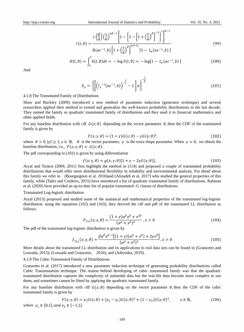
McDonald Log-logistic distribution
Tahir et al. (2014) introduced and studied the McDonald log-logistic distribution and they considered three of the above
extended models of log-logistic distribution, (1) beta log-logistic distribution; (2) Kumaraswamy log-logistic
distribution; and (3) gamma log-logistic or Zografos-Balakrishnan log-logistic distribution.
Using the equations of the cdf and pdf of the McDonald-G family, they obtained the CDF and pdf of the McDonald
log-logistic distribution.
The cdf of the McDonald is given by
𝐹𝑀𝑐𝐿𝐿(𝑥, 𝜃) = 𝐼𝑤(𝑎𝑐−1, 𝑏) =
1
𝐵(𝑎, 𝑏)∫ 𝑤𝑎𝑐
−1−1(1 − 𝑤)𝑏−1𝑑𝑤 (95)𝑤𝑐
0
Where 𝑤 = 𝐶𝐷𝐹 𝑜𝑓 𝐿𝐿 𝑑𝑖𝑠𝑡𝑟𝑖𝑏𝑢𝑡𝑖𝑜𝑛 = [1 + (𝑥
𝛼)−𝛽
]−1
and 𝑎, 𝑏, 𝑐, 𝛼, 𝛽 > 0, where 𝑎, 𝑏, 𝑐, 𝑎𝑛𝑑 𝛽 are shape
parameters while 𝛼 is a scale parameter.
The corresponding pdf of the (95) is given by
𝑓𝑀𝑐𝐿𝐿
(𝑥, 𝜃) = 𝑐
𝐵(𝑎𝑐−1, 𝑏)(𝛽
𝛼) (𝑥
𝛼)𝑎𝛽−1
[1 + (𝑥
𝛼)𝛽
]−(𝑎+1)
[1 − {1 − [1 + (𝑥
𝛼)𝛽
]−1
}
𝑐
]
𝑏−1
, (96)
For a lifetime random variable t, the survivor function, the hazard (failure) rate function, the reversed hazard rate
function, the cumulative hazard rate function and the quantile function of the McDLL distribution are given by
𝑆(𝑡, 𝜃) = 1 − 𝐹(𝑡, 𝜃) = 1 − 𝐼𝑤(𝑎𝑐−1, 𝑏) (97)
ℎ(𝑡, 𝜃) =
𝑐 (𝛽𝛼) (𝑡𝛼)𝑎𝛽−1
[1 − {1 − [1 + (𝑡𝛼)𝛽
]−1
}
𝑐
]
𝑏−1
𝐵(𝑎𝑐−1, 𝑏) [1 + (𝑡𝛼)𝛽
](𝑎+1)
[𝐼𝑤(𝑎𝑐−1, 𝑏) ]
(98)
http://ijsp.ccsenet.org International Journal of Statistics and Probability Vol. 10, No. 3; 2021
109
𝑟(𝑡, 𝜃) =
𝑐 (𝛽𝛼) (𝑡𝛼)𝑎𝛽−1
[1 − {1 − [1 + (𝑡𝛼)𝛽
]−1
}
𝑐
]
𝑏−1
𝐵(𝑎𝑐−1, 𝑏) [1 + (𝑡𝛼)𝛽
](𝑎+1)
[1 − 𝐼𝑤(𝑎𝑐−1, 𝑏) ]
(99)
𝐻(𝑡, 𝜃) = ∫ ℎ(𝑡, 𝜃)𝑑𝑡 = − log 𝑆(𝑡, 𝜃) = − log[1 − 𝐼𝑤(𝑎𝑐−1, 𝑏) ]
𝑡
0
(100)
And
𝑋𝑞 = {[(𝐼𝑞−1(𝑎𝑐−1, 𝑏))
−1𝑐− 1 ]𝛼}
−1𝛽
(101)
4.1.8 The Transmuted Family of Distributions
Shaw and Buckley (2009) introduced a new method of parameter induction (generator technique) and several
researchers applied their method to extend and generalize the well-known probability distributions in the last decade.
They named the family as quadratic transmuted family of distributions and they used it to financial mathematics and
other applied fields.
For any baseline distribution with cdf 𝐺(𝑥; 𝜃) depending on the vector parameter 𝜃, then the CDF of the transmuted
family is given by
𝐹(𝑥; 𝛾, 𝜃) = (1 + 𝛾)𝐺(𝑥; 𝜃) − 𝛾𝐺(𝑥; 𝜃)2, (102)
where 𝜃 > 0, |𝛾| ≥ 1, 𝑥 ∈ ℝ. 𝜃 is the vector parameter, 𝛾 is the extra shape parameter. When 𝛾 = 0, we obtain the
baseline distribution, i.e., 𝐹(𝑥; 𝛾, 𝜃) = 𝐺(𝑥; 𝜃).
The pdf corresponding to (102) is given by using differentiation
𝑓(𝑥; 𝛾, 𝜃) = 𝑔(𝑥; 𝛾, 𝜃)[1 + 𝛾 − 2𝛾𝐺(𝑥; 𝜃)], (103)
Aryal and Tsokos (2009, 2011) first highlight the method in (114) and proposed a couple of transmuted probability
distributions that would offer more distributional flexibility in reliability and environmental analysis. For detail about
this family we refer to (Bourguignon et al. 2016)and (Alizadeh et al. 2017) who studied the general properties of this
family, while (Tahir and Cordeiro, 2015) have introduced a list of quadratic transmuted family of distributions. Rahman
et al. (2020) have provided an up-to-date list of popular transmuted -G classes of distributions.
Transmuted Log-logistic distribution
Aryal (2013) proposed and studied some of the statistical and mathematical properties of the transmuted log-logistic
distribution. using the equations (102) and (103); they derived the cdf and pdf of the transmuted LL distribution as
follows:
𝐹𝑇𝐿𝐿(𝑥; 𝛾, 𝜃) =(1 + 𝛾)𝛼𝛽𝑥𝛽 + 𝑥2𝛽
(𝛼𝛽 + 𝑥𝛽)2 , 𝑥 > 0 (104)
The pdf of the transmuted log-logistic distribution is given by
𝑓𝑇𝐿𝐿(𝑥; 𝛾, 𝜃) =
𝛽𝛼𝛽𝑥𝛽−1[(1 + 𝛾)(𝛼𝛽 + 𝑥𝛽) + 2𝛾𝑥𝛽]
(𝛼𝛽 + 𝑥𝛽)3, 𝑥 > 0 (105)
More details about the transmuted LL distribution and its applications to real data sets can be found in (Granzotto and
Louzada, 2015); (Louzada and Granzotto, 2016); and (Adeyinka, 2019).
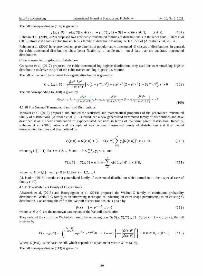
4.1.9 The Cubic Transmuted Family of Distributions
Granzotto et al. (2017) introduced a new parameter induction technique of generating probability distributions called
Cubic Transmutation technique. The reason behind developing of cubic transmuted family was that the quadratic
transmuted distribution captures the complexity of unimodal data but the real-life data become more complex to use
them, and sometimes cannot be fitted by applying the quadratic transmuted family.
For any baseline distribution with cdf 𝐺(𝑥; 𝜃) depending on the vector parameter 𝜃, then the CDF of the cubic
transmuted family is given by
𝐹(𝑥; 𝛾, 𝜃) = 𝛾1𝐺(𝑥; 𝜃) + (𝛾2 − 𝛾1)𝐺(𝑥; 𝜃)2 + (1 − 𝛾2)𝐺(𝑥; 𝜃)
3, 𝑥 ∈ ℝ, (106)
where 𝛾1 ∈ [0,1], 𝑎𝑛𝑑 𝛾2 ∈ [−1,1].
http://ijsp.ccsenet.org International Journal of Statistics and Probability Vol. 10, No. 3; 2021
110
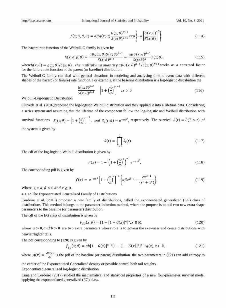
The pdf corresponding to (106) is given by
𝑓(𝑥; 𝛾, 𝜃) = 𝑔(𝑥; 𝜃)[𝛾1 + 2 (𝛾2 − 𝛾1)𝐺(𝑥; 𝜃) + 3(1 − 𝛾2)𝐺(𝑥; 𝜃)2], 𝑥 ∈ ℝ, (107)
Rahman et al. (2019, 2020) proposed two new cubic transmuted families of distributions. On the other hand, Aslam et al.
(2018)introduced another cubic transmuted-G family of distributions using the T-X idea of (Alzaatreh et al, 2013).
Rahman et al. (2020) have provided an up-to-date list of popular cubic transmuted -G classes of distributions. In general,
the cubic transmuted distributions show better flexibility to handle multi-modal data than the quadratic transmuted
distributions.
Cubic transmuted Log-logistic distribution
Granzotto et al. (2017) proposed the cubic transmuted log-logistic distribution. they used the transmuted log-logistic
distribution to derive the pdf of the cubic transmuted log-logistic distribution.
The pdf of the cubic transmuted log-logistic distribution is given by
𝑓𝐶𝑇𝐿𝐿(𝑥; 𝛾, 𝜃) =𝛽𝑥𝛽−1𝑒𝛼
(1 + 𝑒𝛼𝑥𝛽)4[𝛾1(1 − 𝑒
2𝛼𝑥2𝛽) + 𝛾2𝑒𝛼𝑥𝛽(2 − 𝑒𝛼𝑥𝛽) + 3𝑒2𝛼𝑥2𝛽], 𝑥 > 0 (108)
The cdf corresponding to (108) is given by
(109)
4.1.10 The General Transmuted Family of Distributions
Merovci et al. (2016) proposed and studied the statistical and mathematical properties of the generalized transmuted
family of distributions. (Alizadeh et al. 2017) introduced a new generalized transmuted family of distributions and have
described it as a linear combination of exponentiated densities in terms of the same parent distribution. Recently,
Rahman et al. (2018) introduced a couple of new general transmuted family of distributions and they named
k-transmuted families and they defined by
𝐹(𝑥; 𝜃) = 𝐺(𝑥; 𝜃) + [1 − 𝐺(𝑥; 𝜃)]∑𝛾𝑖[𝐺(𝑥; 𝜃)]𝑖
𝑘
𝑖=1
, 𝑥 𝑥 ∈ ℝ, (110)
where 𝛾𝑖 ∈ [−1,1] for 𝑖 = 1,2, … , 𝑘 and −𝑘 ≤ ∑ 𝛾𝑖 ≤ 1,𝑘𝑖=1 and
𝐹(𝑥; 𝜃) = 𝐺(𝑥; 𝜃) + 𝐺(𝑥; 𝜃)∑𝛾𝑖[𝐺(𝑥; 𝜃)]𝑖
𝑘
𝑖=1
, 𝑥 𝑥 ∈ ℝ, (111)
where 𝛾1 ∈ [−1,1] and 𝛾𝑖 ∈ [−1,1]for 𝑖 = 1,2, … , 𝑘.
AL-Kadim (2018) introduced a generalized family of transmuted distribution which turned out to be a special case of
family (110).
4.1.11 The Weibull-G Family of Distributions
Alzaatreh et al. (2013) and Bourguignon et al. (2014) proposed the Weibull-G family of continuous probability
distributions. Weibull-G family is an interesting technique of inducting an extra shape parameter(s) to an existing G
distribution. Considering the cdf of the Weibull distribution which is given by
𝐹(𝑥) = 1 − 𝑒−𝛼𝑥𝛽, 𝑥 > 0 (112)
where 𝛼, 𝛽 > 0 are the unknown parameters of the Weibull distribution.
They defined the cdf of the Weibull-G family by replacing 𝑥 𝑤𝑖𝑡ℎ 𝐺(𝑥; 𝜃)/𝑆(𝑥; 𝜃) [𝑆(𝑥; 𝜃) = 1 − 𝐺(𝑥; 𝜃), ], the cdf
is given by
𝐹(𝑥; 𝛼, 𝛽, 𝜃) = ∫ 𝛼𝛽𝑡𝛽−1𝑒−𝛼𝑡𝛽𝑑𝑡 = 1 − exp {−𝛼 [
𝐺(𝑥; 𝜃)
𝑆(𝑥; 𝜃)]
𝛽
}
𝐺(𝑥;𝜃)1−𝐺(𝑥;𝜃)
0
, 𝑥 ∈ 𝐷 ⊆ ℝ; 𝛼, 𝛽 > 0, (113)
Where 𝐺(𝑥; 𝜃) is the baseline cdf, which depends on a parameter vector 𝜽′ = (𝛼, 𝛽).
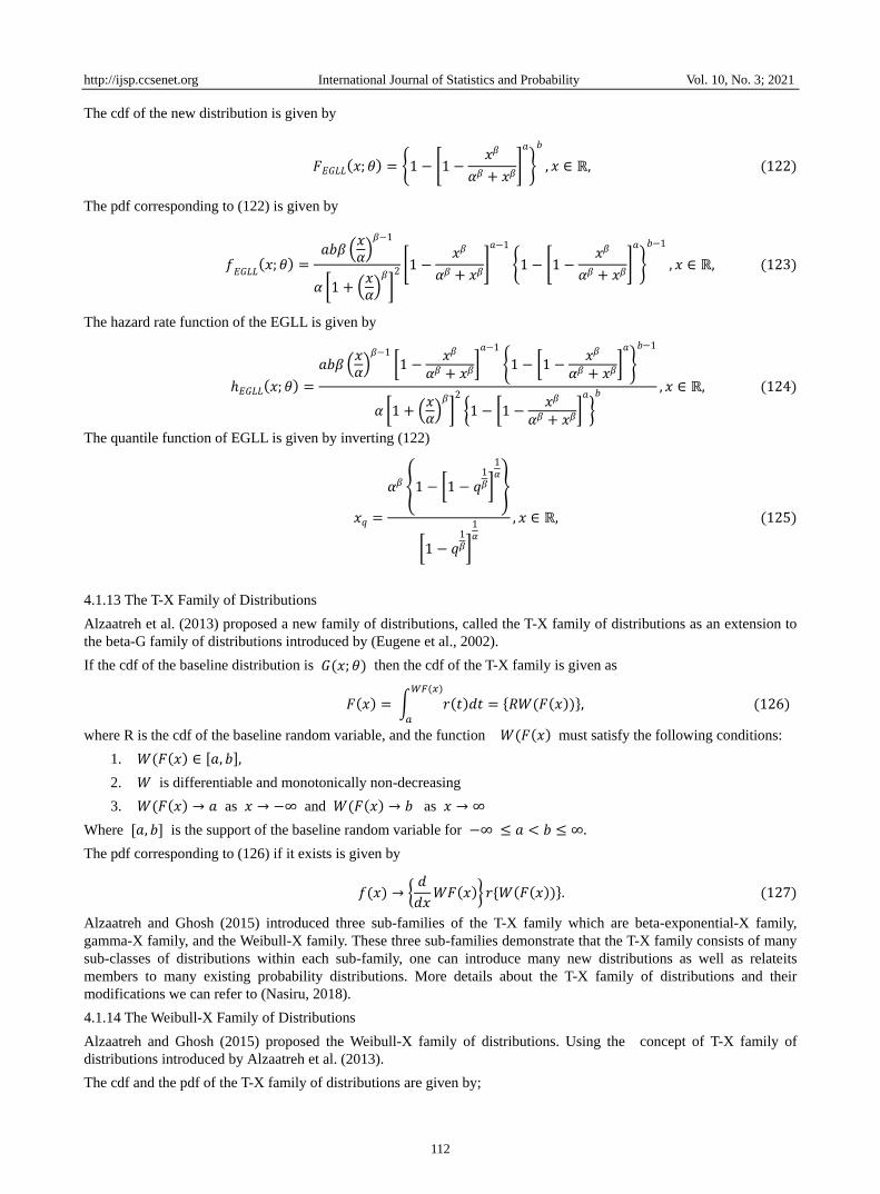
The pdf corresponding to (113) is given by
http://ijsp.ccsenet.org International Journal of Statistics and Probability Vol. 10, No. 3; 2021
111
𝑓(𝑥; 𝛼, 𝛽, 𝜃) = 𝛼𝛽𝑔(𝑥; 𝜃)𝐺(𝑥; 𝜃)𝛽−1
𝑆(𝑥; 𝜃)𝛽+1𝑒𝑥𝑝 {−𝛼 [
𝐺(𝑥; 𝜃)
𝑆(𝑥; 𝜃)]
𝛽
}, (114)
The hazard rate function of the Weibull-G family is given by
ℎ(𝑥; 𝛼, 𝛽, 𝜃) = 𝛼𝛽𝑔(𝑥; 𝜃)𝐺(𝑥; 𝜃)𝛽−1
𝑆(𝑥; 𝜃)𝛽+1= 𝛼𝛽𝐺(𝑥; 𝜃)𝛽−1
𝑆(𝑥; 𝜃)𝛽ℎ(𝑥; 𝜃), (115)
whereℎ(𝑥; 𝜃) = 𝑔(𝑥; 𝜃)/𝑆(𝑥; 𝜃) . 𝑡ℎ𝑒 𝑚𝑢𝑙𝑡𝑖𝑝𝑙𝑦𝑖𝑛𝑔 𝑞𝑢𝑎𝑛𝑡𝑖𝑡𝑦 𝛼𝛽𝐺(𝑥; 𝜃)𝛽−1/𝑆(𝑥; 𝜃)𝛽+1 works as a corrected factor
for the failure rate function of the parent (or baseline) distribution.
The Weibull-G family can deal with general situations in modeling and analysing time-to-event data with different
shapes of the hazard (or failure) rate function. For example, if the baseline distribution is a log-logistic distribution the
𝐺(𝑥; 𝜃)𝛽−1
𝑆(𝑥; 𝜃)𝛽+1= [1 + (
𝑥
𝑠)𝑐
]−1
, 𝑥 > 0 (116)
Weibull-Log-logistic Distribution
Oluyede et al. (2016)proposed the log-logistic Weibull distribution and they applied it into a lifetime data. Considering
a series system and assuming that the lifetime of the component follow the log-logistic and Weibull distribution with
survival functions 𝑆1(𝑡; 𝜃) = [1 + (𝑡
𝑠)𝑐
]−1
, 𝑎𝑛𝑑 𝑆2(𝑡; 𝜃) = 𝑒−𝛼𝑡𝛽 , respectively. The survival 𝑆(𝑡) = 𝑃(𝑇 > 𝑡) of
the system is given by
𝑆(𝑡) = ∏𝑆𝑖(𝑡)
2
𝑖=1
(117)
The cdf of the log-logistic-Weibull distribution is given by
𝐹(𝑥) = 1 − (1 + (𝑥
𝑠)𝑐
)−1
𝑒−𝛼𝑥𝛽, (118)
The corresponding pdf is given by
𝑓(𝑥) = 𝑒−𝛼𝑥𝛽[1 + (
𝑥
𝑠)𝑐
]−1
{𝛼𝛽𝑥𝛽−1 +𝑐𝑥𝑐−1
(𝑠𝑐 + 𝑥𝑐)}, (119)
Where 𝑠, 𝑐, 𝛼, 𝛽 > 0 𝑎𝑛𝑑 𝑥 ≥ 0.
4.1.12 The Exponentiated Generalized Family of Distributions
Cordeiro et al. (2013) proposed a new family of distributions, called the exponentiated generalized (EG) class of
distributions. This method belongs to the parameter induction method, where the purpose is to add two new extra shape
parameters to the baseline (or parameter) distribution.
The cdf of the EG class of distribution is given by
𝐹𝐸𝐺(𝑥; 𝜃) = {1 − [1 − 𝐺(𝑥)]𝑎}𝑏, 𝑥 ∈ ℝ, (120)
where 𝑎 > 0, 𝑎𝑛𝑑 𝑏 > 0 are two extra parameters whose role is to govern the skewness and create distributions with
heavier/lighter tails.
The pdf corresponding to (120) is given by
𝑓𝐸𝐺(𝑥; 𝜃) = 𝑎𝑏[1 − 𝐺(𝑥)]𝑎−1{1 − [1 − 𝐺(𝑥)]𝑎}𝑏−1𝑔(𝑥), 𝑥 ∈ ℝ, (121)
where 𝑔(𝑥) = 𝑑𝐺(𝑥)
𝑑𝑥 is the pdf of the baseline (or parent) distribution. the two parameters in (121) can add entropy to
the center of the Exponentiated Generalized density or possible control both tail weights.
Exponentiated generalized log-logistic distribution
Lima and Cordeiro (2017) studied the mathematical and statistical properties of a new four-parameter survival model
applying the exponentiated generalized (EG) class.
http://ijsp.ccsenet.org International Journal of Statistics and Probability Vol. 10, No. 3; 2021
112
The cdf of the new distribution is given by
𝐹𝐸𝐺𝐿𝐿(𝑥; 𝜃) = {1 − [1 −𝑥𝛽
𝛼𝛽 + 𝑥𝛽]
𝑎
}
𝑏
, 𝑥 ∈ ℝ, (122)
The pdf corresponding to (122) is given by
𝑓𝐸𝐺𝐿𝐿
(𝑥; 𝜃) =𝑎𝑏𝛽 (
𝑥𝛼)𝛽−1
𝛼 [1 + (𝑥𝛼)𝛽
]2 [1 −
𝑥𝛽
𝛼𝛽 + 𝑥𝛽]
𝑎−1
{1 − [1 −𝑥𝛽
𝛼𝛽 + 𝑥𝛽]
𝑎
}
𝑏−1
, 𝑥 ∈ ℝ, (123)
The hazard rate function of the EGLL is given by
ℎ𝐸𝐺𝐿𝐿(𝑥; 𝜃) =
𝑎𝑏𝛽 (𝑥𝛼)𝛽−1
[1 −𝑥𝛽
𝛼𝛽 + 𝑥𝛽]𝑎−1
{1 − [1 −𝑥𝛽
𝛼𝛽 + 𝑥𝛽]𝑎
}
𝑏−1
𝛼 [1 + (𝑥𝛼)𝛽
]2
{1 − [1 −𝑥𝛽
𝛼𝛽 + 𝑥𝛽]𝑎
}𝑏 , 𝑥 ∈ ℝ, (124)
The quantile function of EGLL is given by inverting (122)
𝑥𝑞 =
𝛼𝛽 {1 − [1 − 𝑞1𝛽]
1𝛼
}
[1 − 𝑞1𝛽]
1𝛼
, 𝑥 ∈ ℝ, (125)
4.1.13 The T-X Family of Distributions
Alzaatreh et al. (2013) proposed a new family of distributions, called the T-X family of distributions as an extension to
the beta-G family of distributions introduced by (Eugene et al., 2002).
If the cdf of the baseline distribution is 𝐺(𝑥; 𝜃) then the cdf of the T-X family is given as
𝐹(𝑥) = ∫ 𝑟(𝑡)𝑑𝑡 = {𝑅𝑊(𝐹(𝑥))}, (126)𝑊𝐹(𝑥)
𝑎
where R is the cdf of the baseline random variable, and the function 𝑊(𝐹(𝑥) must satisfy the following conditions:
1. 𝑊(𝐹(𝑥) ∈ [𝑎, 𝑏],
2. 𝑊 is differentiable and monotonically non-decreasing
3. 𝑊(𝐹(𝑥) → 𝑎 as 𝑥 → −∞ and 𝑊(𝐹(𝑥) → 𝑏 as 𝑥 → ∞
Where [𝑎, 𝑏] is the support of the baseline random variable for −∞ ≤ 𝑎 < 𝑏 ≤ ∞.
The pdf corresponding to (126) if it exists is given by
𝑓(𝑥) → {𝑑
𝑑𝑥𝑊𝐹(𝑥)} 𝑟{𝑊(𝐹(𝑥))}. (127)
Alzaatreh and Ghosh (2015) introduced three sub-families of the T-X family which are beta-exponential-X family,
gamma-X family, and the Weibull-X family. These three sub-families demonstrate that the T-X family consists of many
sub-classes of distributions within each sub-family, one can introduce many new distributions as well as relateits
members to many existing probability distributions. More details about the T-X family of distributions and their
modifications we can refer to (Nasiru, 2018).
4.1.14 The Weibull-X Family of Distributions
Alzaatreh and Ghosh (2015) proposed the Weibull-X family of distributions. Using the concept of T-X family of
distributions introduced by Alzaatreh et al. (2013).
The cdf and the pdf of the T-X family of distributions are given by;
http://ijsp.ccsenet.org International Journal of Statistics and Probability Vol. 10, No. 3; 2021
113
𝐹(𝑥) = ∫ 𝑟(𝑡)𝑑𝑡 (128−log [1−𝐺(𝑥)]
𝑎
)
𝑓(𝑥) →𝑔(𝑥)
1 − 𝐺(𝑥)𝑟{− log[1 − 𝐺(𝑥)] = ℎ𝑔(𝑥)𝑟𝐻𝑓(𝑥). (129)
Where ℎ𝑔(𝑥) 𝑎𝑛𝑑 𝐻𝑓(𝑥) are the hazard rate and the cumulative hazard rate functions associated with 𝑔(𝑥).
If a random variable T follows the Weibull distribution with a pdf of
𝑟(𝑡) = (𝛽
𝛼) (𝑡
𝛼) 𝛽−1𝑒−(
𝑡𝛼)
𝛽
, 𝑡 > 0 (130)
The pdf and cdf of the Weibull-X family of distributions is given by
𝑓(𝑥) →𝛽𝑔(𝑥)
𝛼(1 − 𝐺(𝑥))(− log[1 − 𝐺(𝑥)]
𝛼)
𝛽−1
𝑒𝑥𝑝 {−(− log[1 − 𝐺(𝑥)]
𝛼 ) 𝛽} (131)
𝐹(𝑥) = 1 − 𝑒𝑥𝑝 {−(− log[1 − 𝐺(𝑥)]
𝛼 ) 𝛽} , 𝑥 ∈ ℝ (132)
5.1.15 The Exponentiated Kumaraswamy-G family
Lemonte et al. (2013)proposed the exponentiated Kumaraswamy-G family of distributions. The cdf and the pdf of the
EK family are given by
𝐹(𝑥; 𝜃) = [1 − (1 − 𝑥𝛼)𝛽]𝛾, 𝑥 ∈ (0,1) (133)
𝑓(𝑥; 𝜃) = 𝛼𝛽𝛾𝑥𝛼−1(1 − 𝑥𝛼)𝛽−1[1 − (1 − 𝑥𝛼)𝛽−1]𝛾−1
, 𝑥 ∈ (0,1) (134)
where 𝛼𝛽 𝑎𝑛𝑑 𝛾 are extra positive shape parameters. The distribution (134) provides more options for analysing data
restricted to the interval (0,1).
5.1.16 The Generalized Weibull-G Family of Probability Distributions
Cordeiro et al. (2015)proposed a new generalized Weibul-G family of probability distributions and they studied the
mathematical and statistical properties of the family and some special models.
The cdf of the generalized Weibull family is given by
𝐹(𝑥; 𝛼, 𝛽, 𝜃) = 𝛼𝛽∫ 𝑡𝛼−1𝑒−𝛼𝑡𝛽𝑑𝑡 = 1 − exp{−𝛼(− log[1 − 𝐺(𝑥; 𝜃)])𝛽}
−log[1−𝐺(𝑥;𝜃)]
0
(135)
The pdf corresponding to (130) is given by
𝑓(𝑥; 𝛼, 𝛽, 𝜃) =𝛼𝛽𝑔(𝑥; 𝜃)
[1 − 𝐺(𝑥; 𝜃)]{− log[1 − 𝐺(𝑥; 𝜃)]}𝛽−1𝑒𝑥𝑝{−𝛼(− log[1 − 𝐺(𝑥; 𝜃)])𝛽} (136)
The generalized Weibull-Log-logistic Distribution
Cordeiro et al. (2015) introduced the generalized Weibull log-logistic distribution (GWLL).
the pdf of the GWLL with a log-logistic distribution having a scale parameter of a and a shape parameter of b is given
by;
𝑓(𝑥) =𝛼𝛽𝑎𝑥𝑏−1
𝑏𝑎(1 + (
𝑥
𝑏)𝑎
)−1
{log (1 + (𝑥
𝑏)𝑎
)}𝛽−1
𝑒𝑥𝑝 {−𝛼 (log [(1 + (𝑥
𝑏)𝑎
)])𝛽
} (137)
The literature on the generalized log-logistic distribution using generator (or parameter induction) methods is enrich
enough and is also rapidly improving. We now describe the generalization of the log-logistic distribution using
compounding and other methods in the following.
5.1.17 The Gamma Uniform Family of Probability Distributions
Torabi and Hedesh (2016) proposed a new generator approach called the gamma-uniform family of distributions. the
cdf of the family is given by
𝐹(𝑥) = 𝛼𝛽∫𝑒−𝑤𝛽𝑤𝛼−1
Γ(𝛼)𝛽𝛼𝑑𝑤 = 1 − Q {𝛼
𝑥 − 𝑎
𝛽(𝑏 − 𝑥)} , 𝑎 < 𝑥 < 𝑏.
𝑥−𝑎𝑏−𝑥
0
(138)
http://ijsp.ccsenet.org International Journal of Statistics and Probability Vol. 10, No. 3; 2021
114
The pdf and hazard rate function corresponding to (138) are given by
𝑓(𝑥) = (𝑏 − 𝑎)𝑒
−𝑥−𝑎
𝛽(𝑏−𝑥) (𝑥 − 𝑎𝑏 − 𝑥
)𝛼−1
(b − x)2Γ(𝛼)𝛽𝛼, 𝑎 < 𝑥 < 𝑏 (139)
ℎ(𝑥) =(𝑏 − 𝑎)𝑒
−𝑥−𝑎
𝛽(𝑏−𝑥) (𝑥 − 𝑎𝑏 − 𝑥
)𝛼−1
(b − x)2Γ(𝛼,𝑥 − 𝑎
𝛽(𝑏 − 𝑥))𝛽𝛼
, 𝑎 < 𝑥 < 𝑏 (140)
This distribution can be applied for modeling any data set with changing the extra parameters.
4.2 Compounding Methods
The compounding method is a technique that combine two or more existing distributions
4.2.1 The Exponentiated G-Geometric Class
Nadarajah et al. (2015)introduced the exponentiated G-geometric also known as the generalized G-geometric class. If
𝑇[𝐺(𝑥; 𝜏); 𝛾] = 𝐺(𝑥; 𝜏)𝛾 and N be a geometric random variable with failure probability parameter 𝑝 ∈ (0,1) and
probability mass function ℙ(𝑁 = 𝑛) = 𝑞𝑝𝑛−1, 𝑛 = 1,2, … , 𝑝. where p is the success probability.
If we define 𝑋 = 𝑚𝑖𝑛(𝑌1, … , 𝑌𝑁), the unconditional of cdf of the exponentiated G-geometric (EGG) class can follow as
𝐹𝐸𝐺𝐺(𝑥; 𝜃) =∑(1 − 𝑝)𝑝𝑛−1[1 − (1 − 𝐺(𝑥; 𝜏)𝛾)𝑛] =
𝐺(𝑥; 𝜏)𝛾
{1 − 𝑝[1 − 𝐺(𝑥; 𝜏)𝛾]} (141)
∞
𝑛=1
Where 𝛾 > 0, 0 < 𝑝 < 1 are two extra shape parameters. This new family can also be obtained by modification or an
extension of Marshall-Olkin family of distribution by replacing the baseline CDF with its exponentiation and adding
two more extra shape parameters to the original distribution.
The pdf corresponding to (141) is given by
𝑓𝐸𝐺𝐺(𝑥; 𝜃) =
𝛾(1 − 𝑝)𝐺𝛾−1(𝑥; 𝜏)𝑔(𝑥; 𝜏)
{1 − 𝑝[1 − 𝐺(𝑥; 𝜏)𝛾]}2 (142)
The exponentiated log-logistic geometric distribution
Mendoza et al. (2016)proposed and studied the exponentiated log-logistic geometric distribution. they derived some of
the mathematical and statistical properties of the EEG Log-logistic distribution.
If {𝑌𝑖}𝑖=1𝑍 are an i.i.d random variables having the exponentiated log-logistic distribution with cdf and pdf
𝐹𝐸𝐿𝐿(𝑥) = 𝑃𝐸𝐿𝐿({𝑦|𝑦 ≤ 𝑥}) = [(𝑥𝛼)𝛽
1 + (𝑥𝛼)𝛽]
𝛾
𝑓𝑜𝑟 𝑥 ≥ 0 (143)
𝑓𝐸𝐿𝐿(𝑥) =
𝛽𝛾 (𝑥𝛼)𝛽𝛾−1
𝛼 (1 + (𝑥𝛼)𝛽
)𝛾+1 𝑓𝑜𝑟 𝑥 ≥ 0 (144)
where 𝛼, 𝛽, 𝑎𝑛𝑑 𝛾 > 0 are the unknown parameters of the model. For 𝛾 = 1, we obtain as a special case the LL
distribution.
Then,
The conditional density function of EGG log-logistic function for 𝑋1 = min({𝑌𝑖}𝑖=1𝑍 ): is
𝑓(𝑥|𝑧; 𝛾, 𝛼, 𝛽) = 𝑧𝛽𝛾
𝛼(𝑥
𝛼)𝛽𝛾−1
[1 + (𝑥
𝛼 )𝛽
]
−(𝛾+1)
{1 − [1 + (𝑥
𝛼)−𝛽
]
−𝛾
}
𝑧−1
(145)
The pdf of the exponentiated log-logistic geometric type I (ELLGI) distribution reduces to
http://ijsp.ccsenet.org International Journal of Statistics and Probability Vol. 10, No. 3; 2021
115
𝑓𝐸𝐿𝐿𝐺𝐼
(𝑥; 𝜃) = (1−𝑝)𝛽𝛾
𝛼(𝑥
𝛼)𝛽𝛾−1
[1 + (𝑥
𝛼 )𝛽
]−(𝛾+1)
{1 − 𝑝 [1 − {1 + (𝑥
𝛼)−𝛽
}−𝛾
]}−2
(146)
Where 𝑥 > 0, 𝜃 is the vector of parameters ((𝛼, 𝛽, 𝛾 > 0, 𝑎𝑛𝑑 𝑝 ∈ (0,1)..
The cdf corresponding to (146) is given by
𝐹𝐸𝐿𝐿𝐺𝐼(𝑥; 𝜃) = [1 + (𝑥
𝛼 )−𝛽
]−𝛾
{1 − 𝑝 [1 − {1 + (𝑥
𝛼)−𝛽
}−𝛾
]}
−1
, 𝑥 > 0 (147)
The hazard rate function corresponding to (146) is given by
ℎ𝐸𝐿𝐿𝐺𝐼(𝑥; 𝜃) = (1 − 𝑝)𝛽𝛾
𝛼(𝑥
𝛼)𝛽𝛾−1
[1 + (𝑥
𝛼 )𝛽
]−(𝛾+1)
{1 − 𝑝 [1 − {1 + (𝑥
𝛼)−𝛽
}−𝛾
]}
−1
× {1 − 𝑝 [1 − {1 + (𝑥
𝛼)−𝛽
}−𝛾
] − {1 + (𝑥
𝛼)−𝛽
}−𝛾
}
−1
, 𝑥 > 0 (148)
The conditional density function of EGG log-logistic function for 𝑋2 = max({𝑌𝑖}𝑖=1𝑍 ): is
𝑓(𝑥|𝑧; 𝛾, 𝛼, 𝛽) = 𝑧𝛽𝛾
𝛼(𝑥
𝛼)𝛽𝛾−1
[1 + (𝑥
𝛼 )𝛽
]
−(𝛾+1)
[1 + (𝑥
𝛼)−𝛽
]
−𝛾(𝑧−1)
(149)
The pdf of the exponentiated log-logistic geometric type II (ELLGII) distribution reduces to
𝑓𝐸𝐿𝐿𝐺𝐼𝐼
(𝑥; 𝜃) = (1−𝑝)𝛽𝛾
𝛼(𝑥
𝛼)𝛽𝛾−1
[1 + (𝑥
𝛼 )𝛽
]−(𝛾+1)
{1 − 𝑝 [1 + (𝑥
𝛼)−𝛽
]−𝛾
}−2
(150)
Where 𝑥 > 0, 𝜃 is the vector of parameters ((𝛼, 𝛽, 𝛾 > 0, 𝑎𝑛𝑑 𝑝 ∈ (0,1)..
The cdf corresponding to (150) is given by
𝐹𝐸𝐿𝐿𝐺𝐼𝐼(𝑥; 𝜃) = (1 − 𝑝) [1 + (𝑥
𝛼 )−𝛽
]−𝛾
{1 − 𝑝 [1 + (𝑥
𝛼)−𝛽
]−𝛾
}
−1
, 𝑥 > 0 (151)
The hazard rate function corresponding to (150) is given by
ℎ𝐸𝐿𝐿𝐺𝐼𝐼(𝑥; 𝜃) =
(1 − 𝑝)𝛽𝛾𝛼
(𝑥𝛼)𝛽𝛾−1
[1 + (𝑥𝛼 )𝛽
]−(𝛾+1)
{1 − 𝑝 [1 + (𝑥𝛼)−𝛽
]−𝛾
}−2
1 − (1 − 𝑝) [1 + (𝑥𝛼)−𝛽
]−𝛾
{1 − 𝑝 [1 + (𝑥𝛼)−𝛽
]−𝛾
}−1
(152)
4.3 Other Methods
In this section, we present some new techniques for generating new probability distributions.
4.3.1 Khan and Khosa’s Generalized Log-Logistic Distribution
Khan and Khosa (2015) proposed a generalized log-logistic distribution that belongs to the PH family and they
described that it has properties identical to those of log-logistic, and tend to the Weibull in the limit, and they defined
that these features enable the model to handle all kinds of hazard functions.
The pdf, survivor function, hazard rate function, and the cumulative hazard rate function of the Generalized log-logistic
distribution is given by respectively;
𝑓(𝑡; 𝜃) = 𝑘𝜌(𝜌𝑡)𝑘−1
(1 + (𝛾𝑡)𝑘)2, t > 0, (153)
𝑆(𝑡; 𝜃) = [ 1 + (𝛾𝑡)𝑘]−𝑝𝑘
𝛾𝑘 , (154)
ℎ(𝑡; 𝜃) = 𝑘𝜌(𝜌𝑡)𝑘−1
1 + (𝛾𝑥)𝑘, (155)
𝐻(𝑡; 𝜃) =𝑝𝑘
𝛾𝑘log[ 1 + (𝛾𝑡)𝑘], (156)
5. Estimation of the Parameters
In the statistics literature, due to the importance of the LL distribution and its generalizations, the estimation of the
http://ijsp.ccsenet.org International Journal of Statistics and Probability Vol. 10, No. 3; 2021
116
unknown parameters has been widely studied from the two main inferential statistics of thought: frequentists and
Bayesians. From the frequentist approach, there are several different techniques that were proposed for parameter
estimation but the maximum likelihood estimators (MLEs) are commonly used in most of the studies because of their
appealing properties and can be applied when building confidence regions and intervals and also in test statistics.
Although MLE method has been proven to be consistent, asymptotically efficient under very general conditions, it was
found that it breaks down as one parameter tending to cause the likelihood to be infinite, rendering the other parameters
inconsistent and is not applicable to J-shape distributions (Cheng and Amin, 1983). Ranneby, (1984) mentioned that the
MLE is unbound and inefficient in the estimation of the mixtures of continuous distributions and heavy-tailed
distributions. Therefore, to overcome the drawbacks in the MLE method (Cheng and Amin, 1979) proposed a maximum
product of spacings (MPS) estimator to deal with those problems as it will return valid results over a much wider range
of distributions and their generalizations. The method was also developed independently by (Ranneby, 1984).
In this study, we applied the maximum product spacings (MPS) method to estimate the unknown parameters for most of
the generalized distributions discussed in this paper. For more information about the MPS estimator we can refer to
(Cheng and Amin, 1979, 1983; Kawanishi, 2020; Ranneby, 1984; Thongkairat et al. 2018). The MPS estimator is a
general technique used for estimating unknown parameters from observations with continuous univariate distributions
and is an alternative to the MLE method. The log-likelihood for the distribution parameters can be maximized by using
nonlinear likelihood equations obtained by differentiating the log-likelihood or by using software programs and
packages. In this study, we applied the MPS (Maximum Product Spacing) package (version 2.3.1) (Teimouri, 2018)
available in the R programming language to estimate the unknown parameters of the generalized distributions. The
package has been continuously updated and more information can be obtained from
https://cran.rstudio.com/web/packages/MPS/index.html. Currently, Bayesian inference of the log-logistic parameters
and some of its generalizations has also received attention in the literature and some of them are still needs to be
studied.
6. Real-life Data Application
In this section, we compare the performances of some of the generalizations of the log-logistic distribution in Section 5
using a real-life data set. The data represent the survival times of 121 patients with breast cancer obtained from a large
hospital in a period from 1929 to 1938 (Lee and Wang, 2003). The data are:
(154.0, 139.0, 129.0, 129.0, 127.0, 126.0, 125.0, 117.0, 115.0, 111.0, 109.0, 109.0, 105.0, 103.0, 96.0, 93.0, 90.0,
89.0, 88.0, 83.0, 80.0, 78.0, 69.0, 68.0, 67.0, 67.0, 65.0, 65.0, 62.0, 61.0, 60.0, 60.0, 60.0, 59.0, 58.0, 57.0, 56.0,
55.0, 54.0, 52.0, 51.0, 51.0, 51.0, 49.0, 48.0, 47.0, 46.0, 46.0, 45.0, 45.0, 44.0, 43.0, 43.0, 43.0, 42.0, 41.0, 41.0,
41.0, 40.0, 40.0, 40.0, 39.0, 39.0, 38.0, 38.0, 38.0, 37.0, 37.0, 37.0, 35.0, 35.0, 32.0, 31.0, 31.0, 30.0, 29.1, 28.2,
27.9, 24.0, 24.0, 23.6, 23.4, 23.0, 21.1, 21.0, 21.0, 20.9, 20.4, 19.8, 17.9, 17.5, 17.3, 17.2, 16.8, 16.5, 16.3, 16.2,
15.7, 15.5, 14.8, 14.4, 14.4, 13.5, 12.3, 12.2, 11.8, 11.0, 10.3, 8.4, 8.4, 7.5, 7.4, 6.8, 6.6, 6.3, 6.2, 5.6, 5.0, 4.0,
0.3, 0.3)
Table 1. Descriptive statistics of the data
Mean Median Variance Skewness Kurtosis Minimum Maximum
46.33 40 1244.464 1.03 0.35 0.3 154
We fitted the following scale-shape variations of some of the surveyed distributions: The beta log-logistic distribution
(BLL), the Kumaraswamy log-logistic distribution (KWLL), the exponentiated log-logistic distribution (ELL), the
exponentiated generalized log-logistic distribution (EGLL), the Zografos-Balakrishnan log-logistic distribution (ZBLL),
the Marshall-Olkin log-logistic distribution (MO-LL), the Weibull-log-logistic distribution (WLL), the Weibull-X (T-X)
log-logistic distribution (WXLL) , the exponentiated Kumaraswamy log-logistic distribution (EKWLL), the
gamma-uniform log-logistic distribution (GLL), and the Log-logistic (LL) distribution.
Each distribution was fitted by the method of maximum product spacings (MPS). Table 2 gives the values of the MPS
estimates of the model parameters for the BLL, KWLL, ELL, ZBLL, EGLL, MO-LL, WLL, WXLL, EKWLL, GLL,
and LL models fitted to the exceedances of breast cancer data. We estimate the unknown parameters of each model by
maximum product spacings (MPS). There exist many maximization methods in R packages like NM (Nelder-Mead),
BFGS (Broyden-Fletcher Goldfarb-Shanno), NR (Newton-Raphson), BHHH (Berndt-Hall-Hall-Hausman), and SANN
(Simulated-Annealing) methods. In this study, the maximum product spacing estimators (MPS) are computed using
Nelder-Mead optimization (NM) and the measures of goodness of fit AIC, BIC, CAIC, HQIC, Anderson-Darling (A*)
http://ijsp.ccsenet.org International Journal of Statistics and Probability Vol. 10, No. 3; 2021
117
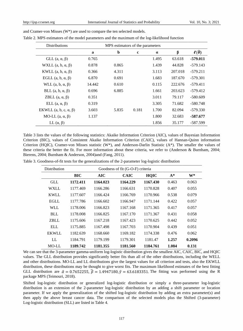
and Cramer-von Misses (W*) are used to compare the ten selected models.
Table 2. MPS estimators of the model parameters and the maximum of the log-likelihood function
Distributions MPS estimators of the parameters
a b c α β 𝓵(�̂�)
GLL (a, α, β) 0.765 1.495 63.618 -579.011
WXLL (a, b, α, β) 0.878 0.865 1.439 44.828 -579.143
KWLL (a, b, α, β) 0.366 4.311 3.113 207.018 -579.211
EGLL (a, b, α, β) 6.870 0.691 1.683 187.670 -579.301
WLL (a, b, α, β) 14.442 0.610 0.115 222.676 -579.411
BLL (a, b, α, β) 0.696 6.885 1.661 203.623 -579.412
ZBLL (a, α, β) 0.351 3.011 79.117 -580.609
ELL (a, α, β) 0.319 3.305 71.682 -580.748
EKWLL (a, b, c, α, β) 3.603 5.835 0.181 1.700 82.094 -579.330
MO-LL (a, α, β) 1.137 1.800 32.683 -587.677
LL (α, β) 1.856 35.177 -587.599
Table 3 lists the values of the following statistics: Akaike Information Criterion (AIC), values of Bayesian Information
Criterion (BIC), values of Consistent Akaike Information Criterion (CAIC), values of Hannan-Quinn information
Criterion (HQIC), Cramer-von Misses statistic (W*), and Anderson-Darlin Statistic (A*). The smaller the values of
these criteria the better the fit. For more information about these criteria, we refer to (Anderson & Burnham, 2004;
Bierens, 2004; Burnham & Anderson, 2004)and (Fang, 2011).
Table 3. Goodness-of-fit tests for the generalizations of the 2-parameter log-logistic distribution
Distribution Goodness of fit (G-O-F) criteria
BIC AIC CAIC HQIC A* W*
GLL 1172.411 1164.023 1164.229 1167.430 0.463 0.063
WXLL 1177.469 1166.286 1166.631 1170.828 0.407 0.055
KWLL 1177.607 1166.424 1166.769 1170.966 0.538 0.079
EGLL 1177.786 1166.602 1166.947 1171.144 0.422 0.057
WLL 1178.006 1166.823 1167.168 1171.365 0.417 0.057
BLL 1178.008 1166.825 1167.170 1171.367 0.431 0.058
ZBLL 1175.606 1167.218 1167.423 1170.625 0.442 0.052
ELL 1175.885 1167.498 1167.703 1170.904 0.439 0.051
EKWLL 1182.639 1168.660 1169.182 1174.338 0.476 0.062
LL 1184.791 1179.199 1179.301 1181.47 1.257 0.2096
MO-LL 1189.742 1181.355 1181.560 1184.761 1.084 0.131
We can see that the 3-parameter gamma-uniform log-logistic distribution gives the smallest AIC, CAIC, BIC, and HQIC
values. The GLL distribution provides significantly better fits than all of the other distributions, including the WELL
and other distributions. MO-LL and LL distributions give the largest values for all criterion and tests, also the EKWLL
distribution, these distributions may be thought to give worst fits. The maximum likelihood estimates of the best fitting
GLL distribution are �̂� = 0.7652255, �̂� = 1.4947180, �̂� = 63.6183351. The fitting was performed using the R
package MPS (Teimouri, 2018).
Shifted log-logistic distribution or generalized log-logistic distribution or simply a three-parameter log-logistic
distribution is an extension of the 2-parameter log-logistic distribution by an adding a shift parameter or location
parameter. If we apply the generalization of the shifted log-logistic distribution by adding an extra parameter(s) and
then apply the above breast cancer data. The comparison of the selected models plus the Shifted (3-parameter)
Log-logistic distribution (SLL) are listed in Table 4.
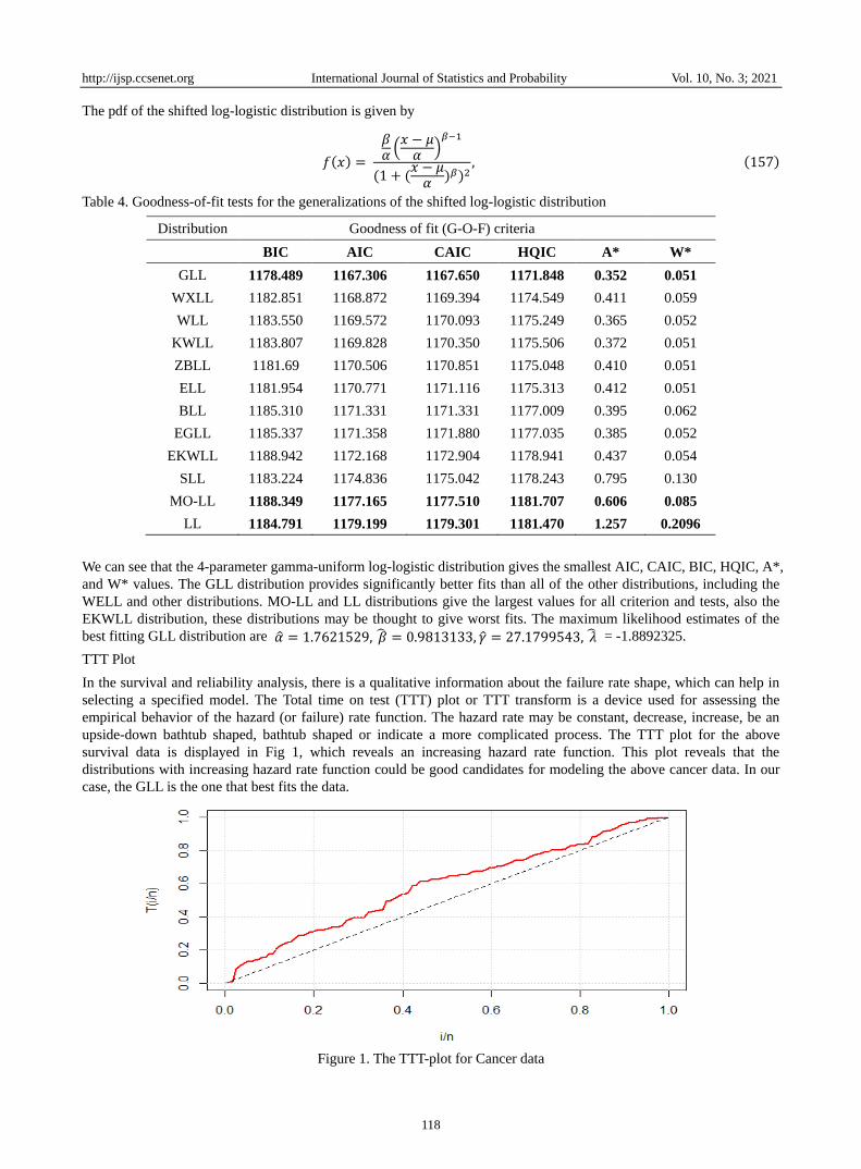
http://ijsp.ccsenet.org International Journal of Statistics and Probability Vol. 10, No. 3; 2021
118
The pdf of the shifted log-logistic distribution is given by
𝑓(𝑥) =
𝛽𝛼(𝑥 − 𝜇𝛼
)𝛽−1
(1 + (𝑥 − 𝜇𝛼
)𝛽)2, (157)
Table 4. Goodness-of-fit tests for the generalizations of the shifted log-logistic distribution
Distribution Goodness of fit (G-O-F) criteria
BIC AIC CAIC HQIC A* W*
GLL 1178.489 1167.306 1167.650 1171.848 0.352 0.051
WXLL 1182.851 1168.872 1169.394 1174.549 0.411 0.059
WLL 1183.550 1169.572 1170.093 1175.249 0.365 0.052
KWLL 1183.807 1169.828 1170.350 1175.506 0.372 0.051
ZBLL 1181.69 1170.506 1170.851 1175.048 0.410 0.051
ELL 1181.954 1170.771 1171.116 1175.313 0.412 0.051
BLL 1185.310 1171.331 1171.331 1177.009 0.395 0.062
EGLL 1185.337 1171.358 1171.880 1177.035 0.385 0.052
EKWLL 1188.942 1172.168 1172.904 1178.941 0.437 0.054
SLL 1183.224 1174.836 1175.042 1178.243 0.795 0.130
MO-LL 1188.349 1177.165 1177.510 1181.707 0.606 0.085
LL 1184.791 1179.199 1179.301 1181.470 1.257 0.2096
We can see that the 4-parameter gamma-uniform log-logistic distribution gives the smallest AIC, CAIC, BIC, HQIC, A*,
and W* values. The GLL distribution provides significantly better fits than all of the other distributions, including the
WELL and other distributions. MO-LL and LL distributions give the largest values for all criterion and tests, also the
EKWLL distribution, these distributions may be thought to give worst fits. The maximum likelihood estimates of the
best fitting GLL distribution are �̂� = 1.7621529, �̂� = 0.9813133, �̂� = 27.1799543, �̂� = -1.8892325.
TTT Plot
In the survival and reliability analysis, there is a qualitative information about the failure rate shape, which can help in
selecting a specified model. The Total time on test (TTT) plot or TTT transform is a device used for assessing the
empirical behavior of the hazard (or failure) rate function. The hazard rate may be constant, decrease, increase, be an
upside-down bathtub shaped, bathtub shaped or indicate a more complicated process. The TTT plot for the above
survival data is displayed in Fig 1, which reveals an increasing hazard rate function. This plot reveals that the
distributions with increasing hazard rate function could be good candidates for modeling the above cancer data. In our
case, the GLL is the one that best fits the data.
Figure 1. The TTT-plot for Cancer data
http://ijsp.ccsenet.org International Journal of Statistics and Probability Vol. 10, No. 3; 2021
119
7. Censored Data and G-Classes of the Log-Logistic Distribution
The generating and extension of the existing probability distributions is an essential topic in survival and reliability
analysis and has been applied in many applications in fields like social sciences, biological sciences, engineering,
economics, physics, chemistry, medicine among others. Extension and generating of an existing probability distribution
might allow to the resulting distribution to accommodate non-monotone forms for the failure rate function. Lai et al
(2013) stated that the time of failure or life can have different interpretations depending on the area applications.
Therefore, we can obtain more flexible distributions for modeling this kind of random variables. On the other hand,
effectiveness and tractability for modeling censored data require, among other things, closed form expressions for the
cumulative distribution function.
The LL distribution has been found to be very useful for modeling and analysing the incomplete (censored and
truncated) data in the area of survival and reliability analysis. The LL distribution is an effective model for censored
data, especially where the hazard rate is non-monotonic (i.e. incidence of an event increases after some finite time and
then slowly decreases). When it comes to the extension of the log-logistic distribution using the G-classes of
distributions, the Kumaraswamy-G family of distributions can be effective and tractable models for incomplete (or
censored) data. The Marshall-Olkin family and the Exponentiated-G family of distributions can also be effective and
tractable models for censored data, provided G is in closed form. However, beta-G and Mc-G distributions may not be
effective or tractable models for censored data since their cumulative distribution functions involve the incomplete beta
function.
8. Concluding Remarks
The LL distribution is one of the most commonly used distributions in survival and reliability analysis, particularly for
events where the hazard rate is non-monotonic. It has also appeared in the literature under other names, such as Fisk
distribution. Various LL extensions and generalizations have been introduced in recent years. In this paper, we have
listed twenty distributions obtained from different generated families and compounding methods on the LL distribution.
We review some of the statistical and mathematical properties of the LL distribution. We expect that these extensions or
generalizations of the LL distributions will be an addition to the art of constructing useful models and lifetime
distributions in general. One can discover easier the type of G-Classes that still is not applied to the LL distribution. The
generalization of log-logistic distribution through generator, compounding and other methods was first applied in the
area of survival and reliability analysis. After that time, several researchers have successfully applied these methods of
generalizations to model lifetime and survival data. At present, these methods are being applied in the areas of
engineering, economics, environmental, medical, hydrology, social science among others to handle more complex data.
9. Future Projects after the Survey
We hope our work will be of value to the statistical and probability community. As for the scope of future work, the
possible future projects are: (1) to propose more new extensions of the LL distribution which have not been attempted;
(2) to review and extend some of the generalized LL distributions, (3) to prepare a review and new developments on
parametric survival models, (4) to derive some mathematical and statistical properties of the new extended distributions,
(5) to estimate the parameters of the new extensions using both the classical and Bayesian approaches; (6) to review the
multi variate, matrix variate and complex variate of the generalized LL distribution; and (6) to applied the new
extensions of the LL distribution into a real-life data sets.
Acknowledgements
We would like to express our heartfelt appreciation to Pan African University, Institute for Basic Sciences, Technology
and Innovation (PAUSTI), and African Union (AU) Commission for their financial support during the research study.
The first author would also like to thank the supervisors for their tireless effort during the study. Also, the authors would
like to thank the editor and reviewers for their careful checking of the details and for the insightful comments and
suggestions that made this manuscript better.
References
Ahmad, Z., Hamedani, G. G., & Butt, N. S. (2019). Recent developments in distribution theory: A brief survey and
some new generalized classes of distributions. Pakistan Journal of Statistics and Operation Research, 15(1), 87–
110. https://doi.org/10.18187/pjsor.v15i1.2803
AL-Kadim, K. A. (2018). {P}roposed {G}eneralized {F}ormula for {T}ransmuted {D}istribution. Journal of
University of Babylon, 26(4), 66–74.
Aldahlan, M. A. (2020). Alpha Power Transformed Log-Logistic Distribution with Application to Breaking Stress Data.
Advances in Mathematical Physics, 2020. https://doi.org/10.1155/2020/2193787
http://ijsp.ccsenet.org International Journal of Statistics and Probability Vol. 10, No. 3; 2021
120
Alexander, C., Cordeiro, G. M., Ortega, E. M. M., & Sarabia, J. M. (2012). Generalized beta-generated distributions.
Computational Statistics and Data Analysis, 56(6), 1880–1897. https://doi.org/10.1016/j.csda.2011.11.015
Alizadeh, M., Merovci, F., & Hamedani, G. G. (2017). Generalized transmuted family of distributions: Properties and
applications. Hacettepe Journal of Mathematics and Statistics, 46(4).
https://doi.org/10.15672/HJMS.201610915478
Alshangiti, A. M., Kayid, M., & Alarfaj, B. (2016). Further results involving Marshall–Olkin log-logistic distribution:
reliability analysis, estimation of the parameter, and applications. SpringerPlus, 5(1).
https://doi.org/10.1186/s40064-016-2007-x
Alzaatreh, A., & Ghosh, I. (2015). On the Weibull-X family of distributions. Journal of Statistical Theory and
Applications, 14(2), 169. https://doi.org/10.2991/jsta.2015.14.2.5
Alzaatreh, A., Lee, C., & Famoye, F. (2013). A new method for generating families of continuous distributions. Metron,
71(1), 63–79. https://doi.org/10.1007/s40300-013-0007-y
Anderson, D., & Burnham, K. (2004). Model selection and multi-model inference. Second. NY: Springer-Verlag,
63(2020), 10.
Aryal, G. R. (2013). Transmuted log-logistic distribution. Journal of Statistics Applications & Probability, 2(1), 11.
Aryal, G. R., & Tsokos, C. P. (2009). On the transmuted extreme value distribution with application. Nonlinear Analysis,
Theory, Methods and Applications, 71(12), e1401–e1407. https://doi.org/10.1016/j.na.2009.01.168
Aryal, G. R., & Tsokos, C. P. (2011). Transmuted Weibull Distribution: A Generalization of the Weibull Probability
Distribution. European Journal of Pure and Applied Mathematics, 4(2), 89–102.
Ashkar, F., & Mahdi, S. (2003). Comparison of two fitting methods for the log‐logistic distribution. Water Resources
Research, 39(8).
Aslam, M., Hussain, Z., & Asghar, Z. (2018). Cubic transmuted-g family of distributions and its properties. Stochastics
and Quality Control, 33(2), 103–112.
Aslam, M., & Jun, C.-H. (2010). A double acceptance sampling plan for generalized log-logistic distributions with
known shape parameters. Journal of Applied Statistics, 37(3), 405–414.
Bacon, R. W. (1993). PRACTITIONERS CORNER: A Note on the Use of the Log‐Logistic Functional Form for
Modelling Saturation Effects. Oxford Bulletin of Economics and Statistics, 55(3), 355–361.
https://doi.org/10.1111/j.1468-0084.1993.mp55003006.x
Barrios, R., & Dios, F. (2012). Exponentiated Weibull distribution family under aperture averaging for Gaussian beam
waves. Optics Express, 20(12), 13055–13064.
Bennett, S. (1983). Log‐logistic regression models for survival data. Journal of the Royal Statistical Society: Series C
(Applied Statistics), 32(2), 165–171.
Bierens, H. J. (2004). Information criteria and model selection. Manuscript, Penn State University.
Bourguignon, M., Ghosh, I., & Cordeiro, G. M. (2016). General Results for the Transmuted Family of Distributions and
New Models. Journal of Probability and Statistics, 2016. https://doi.org/10.1155/2016/7208425
Bourguignon, M., Silva, R. B., & Cordeiro, G. M. (2014). The Weibull-G Family of Probability Distributions. Journal
of Data Science, 12(1), 53–68. https://doi.org/10.6339/JDS.2014.12(1).1210
BRÜEDERL, J., & Diekmann, A. (1995). The log-logistic rate model: Two generalizations with an application to
demographic data. Sociological Methods & Research, 24(2), 158–186.
Burnham, K. P., & Anderson, D. R. (2004). Multimodel inference: understanding AIC and BIC in model selection.
Sociological Methods & Research, 33(2), 261–304.
Casella, G., & Berger, R. L. (2002). Statistical inference (Vol. 2). Duxbury Pacific Grove, CA.
Chaudhary, A. K. (2019). Frequentist Parameter Estimation of Two-Parameter Exponentiated Log-logistic Distribution
BB. NCC Journal, 4(1), 1–8. https://doi.org/10.3126/nccj.v4i1.24727
Chaudhary, A. K., & Kumar, V. (2014). Bayesian Estimation of Three-Parameter Exponentiated Log-logistic
Distribution, 9(2), 66–81.
Chaudhary, A. K., & Ph, D. (2007). Bayesian Analysis of Two-Parameter Exponentiated Log-logistic Distribution, 25(1),
1–12.
http://ijsp.ccsenet.org International Journal of Statistics and Probability Vol. 10, No. 3; 2021
121
Cheng, R. C. H., & Amin, N. A. K. (1979). Maximum product of spacings estimation with applications to the lognormal
distribution. Math Report, 791.
Cheng, R. C. H., & Amin, N. A. K. (1983). Estimating parameters in continuous univariate distributions with a shifted
origin. Journal of the Royal Statistical Society: Series B (Methodological), 45(3), 394–403.
Choudhury, A. (2005). A simple derivation of moments of the exponentiated Weibull distribution. Metrika, 62(1), 17–
22.
Collatt, D. (2003). David Collett Modelling Survival Data in Medical Research - Copy.pdf.
Cordeiro, G. M., & de Castro, M. (2011). A new family of generalized distributions. Journal of Statistical Computation
and Simulation, 81(7), 883–898. https://doi.org/10.1080/00949650903530745
Cordeiro, G. M., Edwin, E. M., & Ramires, T. G. (2015). A new generalized Weibull family of distributions:
mathematical properties and applications. Journal of Statistical Distributions and Applications, 2(1).
https://doi.org/10.1186/s40488-015-0036-6
Cordeiro, G. M., & Nadarajah, S. (2011). Closed-form expressions for moments of a class of beta generalized
distributions. Brazilian Journal of Probability and Statistics, 25(1), 14–33. https://doi.org/10.1214/09-BJPS109
Cordeiro, G. M., Ortega, E. M. M., & Cunha, D. C. C. (2013). The Exponentiated Generalized Class of Distributions.
Journal of Data Science, 11(1), 109–142. https://doi.org/10.6339/JDS.2013.11(1).1086
De Brito, C. R., Rêgo, L. C., De Oliveira, W. R., & Gomes-Silva, F. (2019). Method for generating distributions and
classes of probability distributions: The univariate case. Hacettepe Journal of Mathematics and Statistics, 48(3),
897–930. https://doi.org/10.15672/HJMS.2018.619
de Santana, T. V. F., Ortega, E. M. M., Cordeiro, G. M., & Silva, G. O. (2012). {T}he
{K}umaraswamy-{L}og-{L}ogistic {D}istribution. {J}ournal of {S}tatistical {T}heory and {A}pplications, 11(3),
265–291.
Dey, S., Kumar, D., Anis, M. Z., Nadarajah, S., & Okorie, I. (2021). A Review of Transmuted Distributions. Journal of
the Indian Society for Probability and Statistics. https://doi.org/10.1007/s41096-021-00096-0
Diekmann, A. (1992). The log-logistic distribution as a model for social diffusion processes. Journal of Scientific and
Industrial Research, 51, 285–290.
Ekawati, D., Warsono, W., & Kurniasari, D. (2015). On the Moments, Cumulants, and Characteristic Function of the
Log-Logistic Distribution. IPTEK The Journal for Technology and Science, 25(3).
Eugene, N., Lee, C., & Famoye, F. (2002). BETA-NORMAL DISTRIBUTION AND ITS APPLICATIONS.
Communications in Statistics - Theory and Methods, 31(4), 497–512. https://doi.org/10.1081/STA-120003130
Fang, Y. (2011). Asymptotic equivalence between cross-validations and Akaike information criteria in mixed-effects
models. Journal of Data Science, 9(1), 15–21.
Fisk, P. R. (1961). The graduation of income distributions. Econometrica: Journal of the Econometric Society, 171–185.
Ghitany, M. E. (1998). On a recent generalization of gamma distribution. Communications in Statistics - Theory and
Methods, 27(1), 223–233. https://doi.org/10.1080/03610929808832662
Gholam, H. H. (2013). Characterizations of exponentiated distributions. Pakistan Journal of Statistics and Operation
Research, 9(1), 17–24. https://doi.org/10.18187/pjsor.v9i1.435
Gompertz, B. (1825). XXIV. On the nature of the function expressive of the law of human mortality, and on a new mode
of determining the value of life contingencies. In a letter to Francis Baily, Esq. FRS &c. Philosophical
Transactions of the Royal Society of London, (115), 513–583.
Granzotto, D. C. T., Louzada, F., & Balakrishnan, N. (2017). Cubic rank transmuted distributions: inferential issues and
applications. Journal of Statistical Computation and Simulation, 87(14), 2760–2778.
https://doi.org/10.1080/00949655.2017.1344239
Granzotto, D. C. T., & Louzada, F. (2015). The Transmuted Log-Logistic Distribution: Modeling, Inference, and an
Application to a Polled Tabapua Race Time up to First Calving Data. Communications in Statistics - Theory and
Methods, 44(16), 3387–3402. https://doi.org/10.1080/03610926.2013.775307
Gui, W. (2013). Marshall-olkin extended log-logistic distribution and its application in minification processes. Applied
Mathematical Sciences, 7(77–80), 3947–3961. https://doi.org/10.12988/ams.2013.35268
Gupta, R. C., & Akman, H. O. (1995). On the reliability studies of a weighted inverse Gaussian model. Journal of
http://ijsp.ccsenet.org International Journal of Statistics and Probability Vol. 10, No. 3; 2021
122
Statistical Planning and Inference, 48(1), 69–83.
Gupta, R. C., Akman, O., & Lvin, S. (1999). A study of log‐logistic model in survival analysis. Biometrical Journal:
Journal of Mathematical Methods in Biosciences, 41(4), 431–443.
Gupta, R. C., Gupta, P. L., & Gupta, R. D. (1998). Modeling failure time data by Lehman alternatives. Communications
in Statistics-Theory and Methods, 27(4), 887–904.
Gupta, R. D., & Kundu, D. (1999). Theory & methods: Generalized exponential distributions. Australian & New
Zealand Journal of Statistics, 41(2), 173–188.
Gupta, R. D., & Kundu, D. (2001). Exponentiated exponential family: an alternative to gamma and Weibull
distributions. Biometrical Journal: Journal of Mathematical Methods in Biosciences, 43(1), 117–130.
Gupta, R. D., & Kundu, D. (2009). Introduction of shape/skewness parameter (s) in a probability distribution. J Probab
Stat Sci, 7, 153–171.
Gupta, R. D., & Kundu, D. (2002). Generalized exponential distributions: statistical inferences. Journal of Statistical
Theory and Applications, 1(1), 101–118.
Jones, M. C. (2009). Kumaraswamy’s distribution: A beta-type distribution with some tractability advantages. Statistical
Methodology, 6(1), 70–81. https://doi.org/10.1016/j.stamet.2008.04.001
Jones, M. C. (2004). Families of distributions arising from distributions of order statistics. Test, 13(1), 1–43.
Kawanishi, T. (2020). Maximum likelihood and the maximum product of spacings from the viewpoint of the method of
weighted residuals. Computational and Applied Mathematics, 39(3). https://doi.org/10.1007/s40314-020-01179-7
Khan, S. A., & Khosa, S. K. (2015). Generalized log-logistic proportional hazard model with applications in survival
analysis. Journal of Statistical Distributions and Applications, 3(1). https://doi.org/10.1186/s40488-016-0054-z
Kleiber, C., & Kotz, S. (2003). Statistical size distributions in economics and actuarial sciences (Vol. 470). John Wiley
& Sons.
Kumaraswamy, P. (1980). A generalized probability density function for double-bounded random processes. Journal of
Hydrology, 46(1–2), 79–88. https://doi.org/10.1016/0022-1694(80)90036-0
Lee, C., Famoye, F., & Alzaatreh, A. Y. (2013). Methods for generating families of univariate continuous distributions
in the recent decades. Wiley Interdisciplinary Reviews: Computational Statistics, 5(3), 219–238.
https://doi.org/10.1002/wics.1255
Lee, E. T., & Wang, J. (2003). Statistical methods for survival data analysis (Vol. 476). John Wiley & Sons.
Lehmann, E. L. (1953). The power of rank tests. The Annals of Mathematical Statistics, 23–43.
Lemonte, A. J. (2014). The beta log-logistic distribution. Brazilian Journal of Probability and Statistics, 28(3), 313–332.
https://doi.org/10.1214/12-BJPS209
Lemonte, A. J., Barreto-Souza, W., & Cordeiro, G. M. (2013). The exponentiated Kumaraswamy distribution and its
log-transform. Brazilian Journal of Probability and Statistics, 27(1), 31–53. https://doi.org/10.1214/11-BJPS149
Lemonte, A. J., & Cordeiro, G. M. (2013). An extended Lomax distribution. Statistics, 47(4), 800–816.
https://doi.org/10.1080/02331888.2011.568119
Li, R., & Nadarajah, S. (2020). A review of Student’s t distribution and its generalizations. Empirical Economics, 58(3),
1461–1490. https://doi.org/10.1007/s00181-018-1570-0
Lima, S. R., & Cordeiro, G. M. (2017). The extended log-logistic distribution: Properties and application. Anais Da
Academia Brasileira de Ciencias, 89(1), 3–17. https://doi.org/10.1590/0001-3765201720150579
Little, C. L., Adams, M. R., Anderson, W. A., & Cole, M. B. (1994). Application of a log-logistic model to describe the
survival of Yersinia enterocolitica at sub-optima pH and temperature. International Journal of Food Microbiology,
22(1), 63–71.
Louzada, F., & Granzotto, D. C. T. (2016). The transmuted log-logistic regression model: a new model for time up to
first calving of cows. Statistical Papers, 57(3), 623–640. https://doi.org/10.1007/s00362-015-0671-5
Mahdavi, A., & Kundu, D. (2017). A new method for generating distributions with an application to exponential
distribution. Communications in Statistics - Theory and Methods, 46(13), 6543–6557.
https://doi.org/10.1080/03610926.2015.1130839
Malik, A. S., & Ahmad, S. P. (2020). An Extension of Log-Logistic Distribution for Analyzing Survival Data. Pakistan
http://ijsp.ccsenet.org International Journal of Statistics and Probability Vol. 10, No. 3; 2021
123
Journal of Statistics and Operation Research, 16(4), 789–801. https://doi.org/10.18187/PJSOR.V16I4.2961
Marshall, A. W., & Olkin, I. (1997). A new method for adding a parameter to a family of distributions with application
to the exponential and Weibull families. Biometrika, 84(3), 641–652.
McDonald, J. B. (2008). Some generalized functions for the size distribution of income. In Modeling income
distributions and Lorenz curves (pp. 37–55). Springer.
Mendoza, N. V. R., Ortega, E. M. M., & Cordeiro, G. M. (2016). The exponentiated-log-logistic geometric distribution:
Dual activation. Communications in Statistics - Theory and Methods, 45(13), 3838–3859.
https://doi.org/10.1080/03610926.2014.909937
Merovci, F., Alizadeh, M., & Hamedani, G. G. (2016). Another generalized transmuted family of distributions:
Properties and applications. Austrian Journal of Statistics, 45(3), 71–93. https://doi.org/10.17713/ajs.v45i3.109
Midhu, N. N., Sankaran, P. G., & Nair, N. U. (2013). A class of distributions with the linear mean residual quantile
function and it’s generalizations. Statistical Methodology, 15, 1–24.
Mudholkar, G. S., & Hutson, A. D. (1996). The exponentiated Weibull family: some properties and a flood data
application. Communications in Statistics--Theory and Methods, 25(12), 3059–3083.
Mudholkar, G. S., & Srivastava, D. K. (1993). Exponentiated Weibull family for analyzing bathtub failure-rate data.
IEEE Transactions on Reliability, 42(2), 299–302.
Mudholkar, G. S., Srivastava, D. K., & Freimer, M. (1995). The exponentiated Weibull family: A reanalysis of the
bus-motor-failure data. Technometrics, 37(4), 436–445.
Muthulakshmi, S. (2013). Double sampling plan for Truncated Life test based on Kumaraswamy-Log-Logistic
Distribution. IOSR Journal of Mathematics, 7(4), 29–37. https://doi.org/10.9790/5728-0742937
Nadarajah, S., Cordeiro, G. M., & Ortega, E. M. M. (2013). The exponentiated Weibull distribution: A survey.
Statistical Papers, 54(3), 839–877. https://doi.org/10.1007/s00362-012-0466-x
Nadarajah, S., Cordeiro, G. M., & Ortega, E. M. M. (2015a). The exponentiated G geometric family of distributions.
Journal of Statistical Computation and Simulation, 85(8), 1634–1650.
https://doi.org/10.1080/00949655.2014.885977
Nadarajah, S., Cordeiro, G. M., & Ortega, E. M. M. (2015b). The zografos-balakrishnan-G family of distributions:
Mathematical properties and applications. Communications in Statistics - Theory and Methods, 44(1), 186–215.
https://doi.org/10.1080/03610926.2012.740127
Nadarajah, S., & Kotz, S. (2006). The exponentiated type distributions. Acta Applicandae Mathematica, 92(2), 97–111.
Nandram, B. (1989). Discrimination between the complementary log-log and logistic model for ordinal data.
Communications in Statistics-Theory and Methods, 18(6), 2155–2164.
Nasiru, S. (2018). A New Generalization of Transformed-Transformer Family of Distributions. Retrieved from
http://ir.jkuat.ac.ke:8080/bitstream/handle/123456789/4674/MS400-0002-16%28THESIS
FINAL%29.pdf?sequence=1&isAllowed=y
Nasiru, S., Mwita, P. N., & Ngesa, O. (2019). Alpha power transformed Fréchet distribution. Applied Mathematics and
Information Sciences, 13(1), 129–141. https://doi.org/10.18576/AMIS/130117
Oluyede, B. O., Foya, S., Warahena-Liyanage, G., & Huang, S. (2016). The log-logistic weibull distribution with
applications to lifetime data. Austrian Journal of Statistics, 45(3), 43–69. https://doi.org/10.17713/ajs.v45i3.107
Pham, H., & Lai, C. D. (2007). On recent generalizations of the Weibull distribution. IEEE Transactions on Reliability,
56(3), 454–458. https://doi.org/10.1109/TR.2007.903352
Prentice, R. L. (1976). A Generalization of the Probit and Logit Methods for Dose Response Curves. Biometrics, 32(4),
761–768. https://doi.org/10.2307/2529262
Prentice, R. L., & Kalbfleisch, J. D. (1979). Hazard rate models with covariates. Biometrics, 25–39.
Rahman, M. M., Al-Zahrani, B., & Shahbaz, M. Q. (2018). A general transmuted family of distributions. Pakistan
Journal of Statistics and Operation Research, 14(2), 463–481. https://doi.org/10.18187/pjsor.v14i2.2334
Rahman, M. M., Al-Zahrani, B., & Shahbaz, M. Q. (2019). Cubic transmuted Weibull distribution: properties and
applications. Annals of Data Science, 6(1), 83–102.
Rahman, M. M., Al-Zahrani, B., & Shahbaz, M. Q. (2020). Cubic transmuted pareto distribution. Annals of Data
Science, 7(1), 91–108.
http://ijsp.ccsenet.org International Journal of Statistics and Probability Vol. 10, No. 3; 2021
124
Rahman, M. M., Al-Zahrani, B., Shahbaz, S. H., & Shahbaz, M. Q. (2020). Transmuted probability distributions: A
review. Pakistan Journal of Statistics and Operation Research, 16(1), 83–94.
https://doi.org/10.18187/PJSOR.V16I1.3217
Ramos, M. W. A. (2013). The Zografos-Balakrishnan Log-Logistic Distribution. Properties and Application, Journal of
Statistical Theory and Applications, 12(3), 244–255.
Ranneby, B. (1984). The maximum spacing method. An estimation method related to the maximum likelihood method.
Scandinavian Journal of Statistics, 93–112.
Rao, G. S., Kantam, R. R. L., Rosaiah, K., & Prasad, S. V. (2012). Reliability test plans for type-II exponentiated
log-logistic distribution. Journal of Reliability and Statistical Studies, 5(1), 55–64.
Reath, J., Dong, J., & Wang, M. (2018). Improved parameter estimation of the log-logistic distribution with applications.
Computational Statistics, 33(1), 339–356. https://doi.org/10.1007/s00180-017-0738-y
Rosaiah, K., Kantam, R. R. L., & Kumar, S. (2006). Reliability test plans for exponentiated log-logistic distribution.
Stochastics and Quality Control, 21(2), 279–289.
Rowinski, P. M., Strupczewski, W. G., & Singh, V. P. (2002). A note on the applicability of log-Gumbel and log-logistic
probability distributions in hydrological analyses: I. Known pdf. Hydrological Sciences Journal, 47(1), 107–122.
Samuel, A. F. (2019). On Transmuted Four Parameters Generalized Log-Logistic Distribution. International Journal of
Statistical Distributions and Applications, 5(2), 32. https://doi.org/10.11648/j.ijsd.20190502.12
Shakhatreh, M. K. (2018). A new three-parameter extension of the log-logistic distribution with applications to survival
data. Communications in Statistics - Theory and Methods, 47(21), 5205–5226.
https://doi.org/10.1080/03610926.2017.1388399
Shakil, M., & Ahsanullah, M. (2012). Review on Order Statistics and Record Values from F^{α} Distributions. Pakistan
Journal of Statistics and Operation Research, 101–120.
Shaw, W. T., & Buckley, I. R. C. (2009). The alchemy of probability distributions: beyond Gram-Charlier expansions,
and a skew-kurtotic-normal distribution from a rank transmutation map, 1–8. Retrieved from
http://arxiv.org/abs/0901.0434
Singh, K. P., Lee, C. M. ‐., & George, E. O. (1988). On Generalized Log‐Logistic Model for Censored Survival Data.
Biometrical Journal, 30(7), 843–850. https://doi.org/10.1002/bimj.4710300714
Singh, U., Gupta, P. K., & Upadhyay, S. K. (2005). Estimation of three-parameter exponentiated-Weibull distribution
under type-II censoring. Journal of Statistical Planning and Inference, 134(2), 350–372.
Tahir, M.H., Mansoor, M., Zubair, M., & Hamedani, G. G. (2014). McDonald log-logistic distribution with an
application to breast cancer data. Journal of Statistical Theory and Applications, 13(1), 65.
https://doi.org/10.2991/jsta.2014.13.1.6
Tahir, M. H., & Cordeiro, G. M. (2015). Compounding of distributions: a survey and new generalized classes. Journal
of Statistical Distributions and Applications (Vol. 3). Journal of Statistical Distributions and Applications.
https://doi.org/10.1186/s40488-016-0052-1
Tahir, Muhammad H., & Nadarajah, S. (2015). Parameter induction in continuous univariate distributions:
Well-established G families. Anais Da Academia Brasileira de Ciencias, 87(2), 539–568.
https://doi.org/10.1590/0001-3765201520140299
Teimouri, M. (2018). MPS: An R package for modelling new families of distributions. ArXiv Preprint
ArXiv:1809.02959.
Thongkairat, S., Yamaka, W., & Sriboonchitta, S. (2018). Maximum product spacings method for the estimation of
parameters of linear regression. Journal of Physics: Conference Series, 1053(1).
https://doi.org/10.1088/1742-6596/1053/1/012110
Tomy, L., Jose, M., & Veena, G. (2020). A review on recent generalizations of exponential distribution, (October).
https://doi.org/10.15406/bbij.2020.09.00313
Torabi, H., & Hedesh, N. M. (2016). The gamma-uniform distribution and its applications Kybernetika Hamzeh Torabi ;
Narges Montazeri Hedesh, (January 2012).
Verhulst, P.-F. (1838). Notice sur la loi que la population suit dans son accroissement. Corresp. Math. Phys., 10, 113–
126.
http://ijsp.ccsenet.org International Journal of Statistics and Probability Vol. 10, No. 3; 2021
125
Verhulst, P. (1847). Deuxième mémoire sur la loi d’accroissement de la population. Mémoires de l’académie Royale
Des Sciences, Des Lettres et Des Beaux-Arts de Belgique, 20, 1–32.
Verhulst, P. F. (1845). Recherches Mathématiques sur La Loi D’Accroissement de la Population, Nouveaux Mémoires
de l’Académie Royale des Sciences et Belles-Lettres de Bruxelles, 18, Art. 1, 1-45. N.
Zografos, K., & Balakrishnan, N. (2009). On families of beta- and generalized gamma-generated distributions and
associated inference. Statistical Methodology, 6(4), 344–362. https://doi.org/10.1016/j.stamet.2008.12.003
Copyrights
Copyright for this article is retained by the author(s), with first publication rights granted to the journal.
This is an open-access article distributed under the terms and conditions of the Creative Commons Attribution license
(http://creativecommons.org/licenses/by/4.0/).