Generalized Linear ModelsLogistic RegressionLog-Linear Models

© G. Quinn & M. Keough, 2004

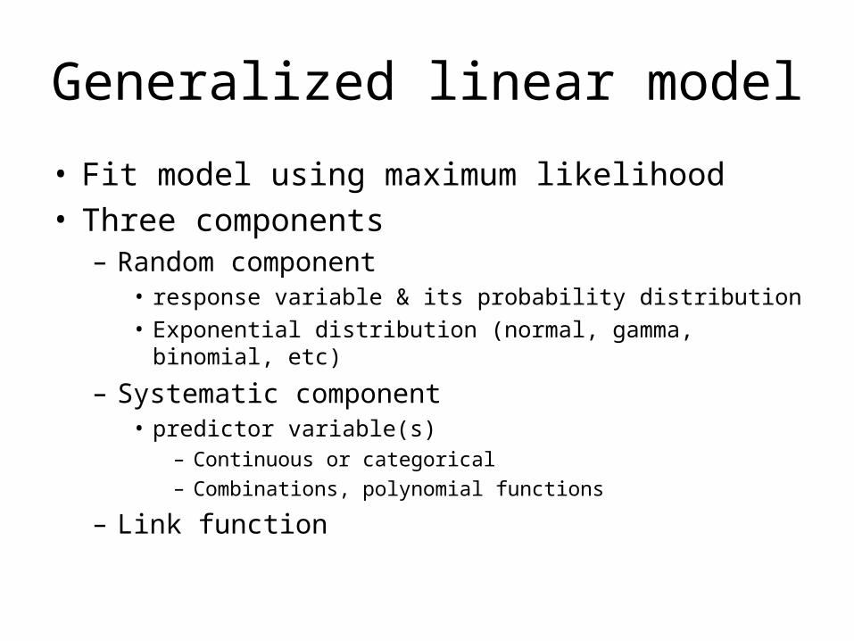
Generalized linear model

• Fit model using maximum likelihood• Three components

– Random component • response variable & its probability distribution• Exponential distribution (normal, gamma, binomial, etc)

– Systematic component• predictor variable(s)

– Continuous or categorical

– Combinations, polynomial functions

– Link function

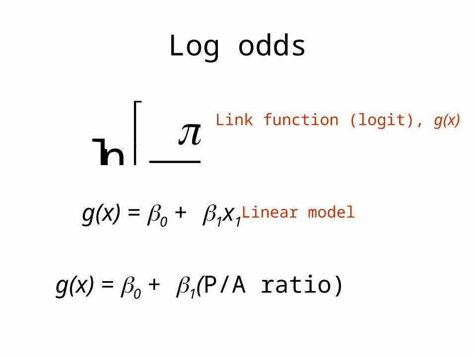
Link function

• Links expected value of Y to predictors

0 1 1 2 2( ) ...g X X

Three common link functions

• Identity link– g() = – Models mean or expected value of Y– Standard linear models

• Log link– g() = log()– Used for count data, which cannot be negative

• Logit link– g() = log(/(1-))– Used for binary data and logistic regression

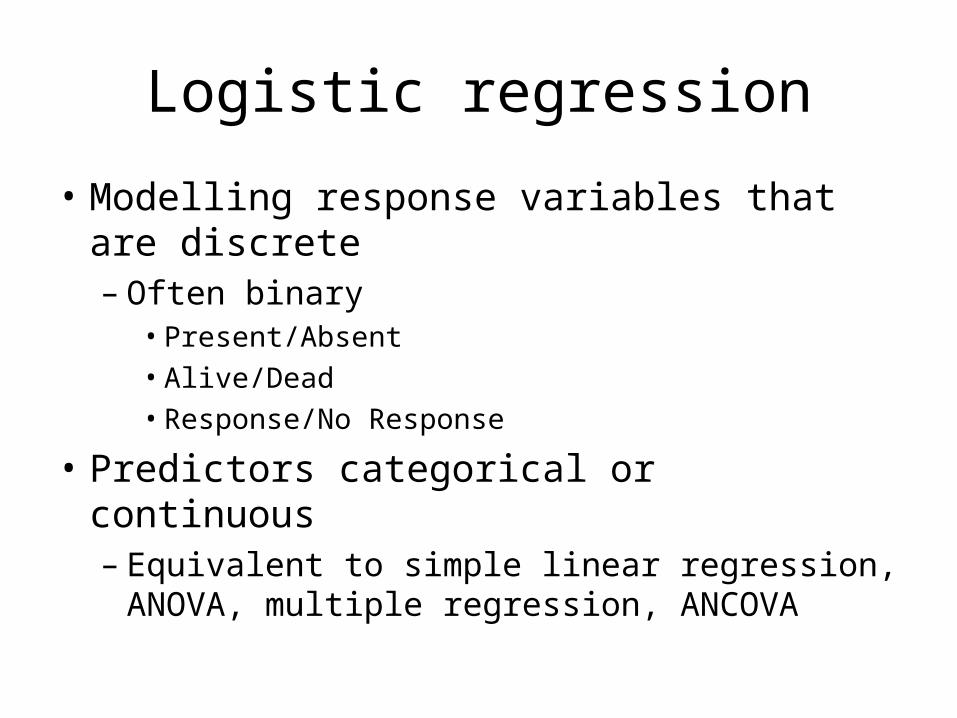
Logistic regression

• Modelling response variables that are discrete– Often binary

• Present/Absent• Alive/Dead• Response/No Response

• Predictors categorical or continuous– Equivalent to simple linear regression,

ANOVA, multiple regression, ANCOVA

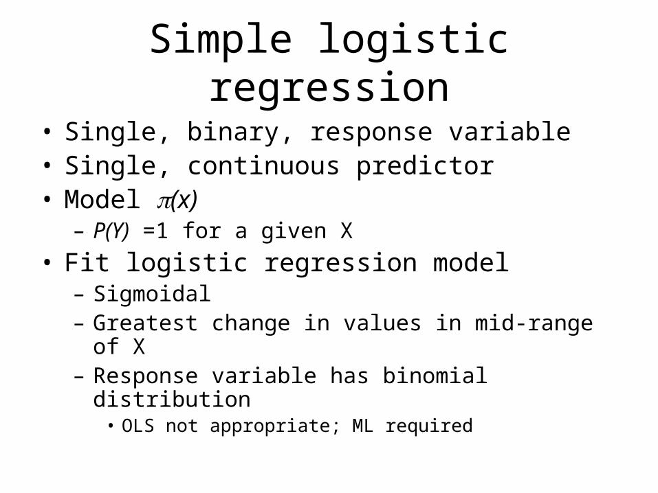
Simple logistic regression

• Single, binary, response variable• Single, continuous predictor• Model (x)

– P(Y) =1 for a given X

• Fit logistic regression model– Sigmoidal– Greatest change in values in mid-range of X– Response variable has binomial distribution

• OLS not appropriate; ML required

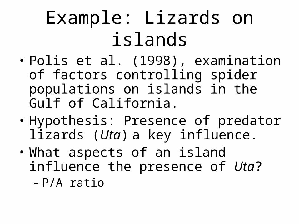
Example: Lizards on islands

• Polis et al. (1998), examination of factors controlling spider populations on islands in the Gulf of California.

• Hypothesis: Presence of predator lizards (Uta) a key influence.

• What aspects of an island influence the presence of Uta?– P/A ratio

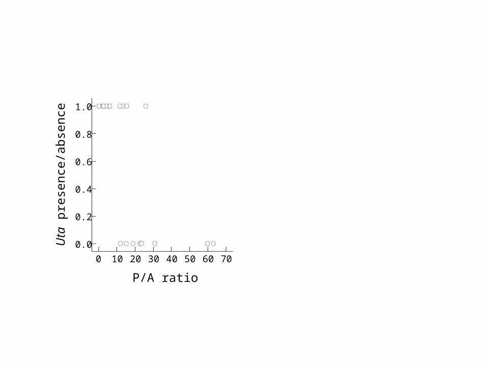
0 10 20 30 40 50 60 70

P/A ratio

0.0

0.2

0.4

0.6

0.8

1.0

Uta

pre

senc

e/ab

senc

e

The logistic model

0 1

0 1

( )1

x

x

ex

e

0 and 1 are parameters to be estimated•Slope and intercept

A simpler model

• Calculate odds – P(event)/P(1-event)

– P(yi = 1)/P(yi = 0)

( )

1 ( )

x

x

( )ln

1 ( )

x

x

Log odds

Link function (logit), g(x)

g(x) = 0 + 1x1Linear model

g(x) = 0 + 1(P/A ratio)

Interpretation

1 is the rate of change in the log(odds) for a unit change in X

• More often expressed as the Odds Ratio– Change in odds for unit change in X

–e

0 is the intercept

– not often of biological interest

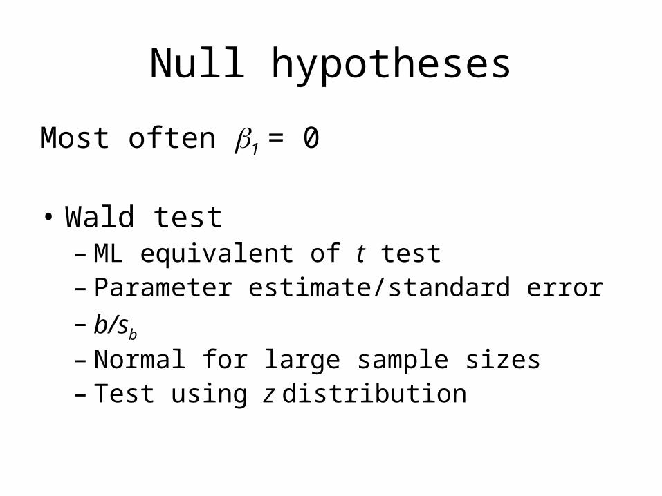
Null hypotheses

Most often 1 = 0

• Wald test– ML equivalent of t test– Parameter estimate/standard error– b/sb

– Normal for large sample sizes– Test using z distribution

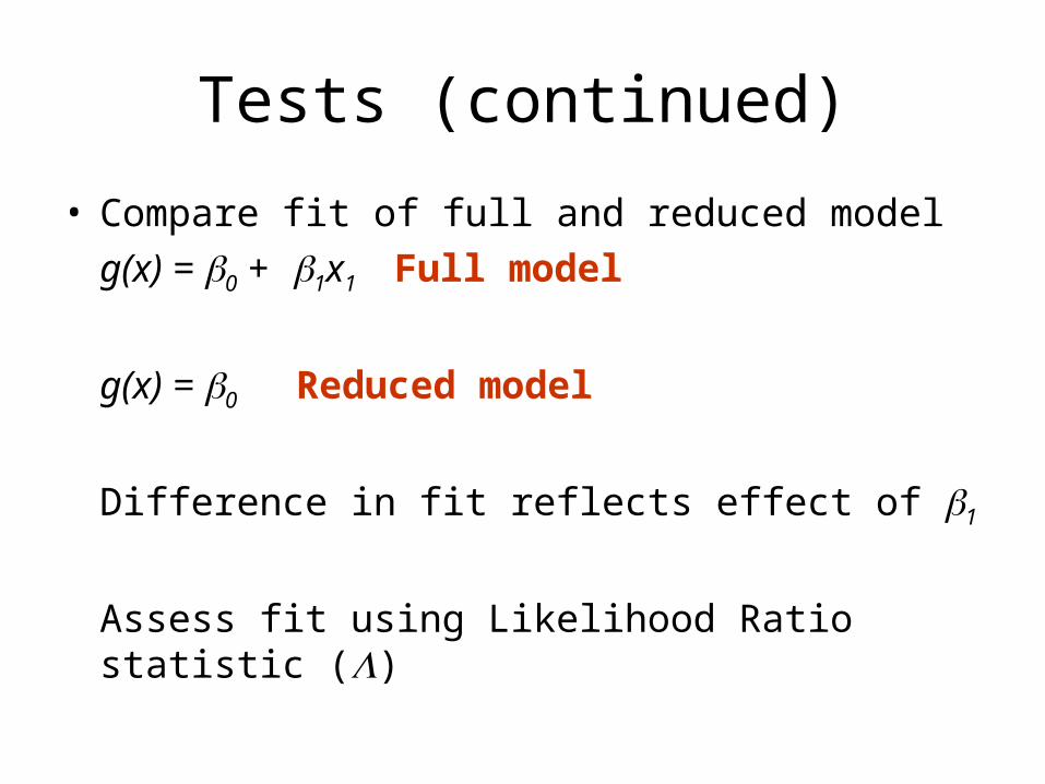
Tests (continued)

• Compare fit of full and reduced model

g(x) = 0 + 1x1 Full model

g(x) = 0 Reduced model

Difference in fit reflects effect of 1

Assess fit using Likelihood Ratio statistic ()

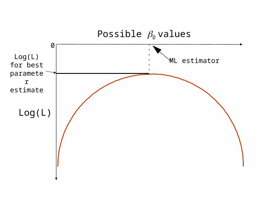
Log(L)

ML estimator

Possible 0 values

Log(L) for best

parameter estimate

0

1 values0 values

Log(L)

Log(L) for best

parameter estimate

Tests (continued)

is the ratio of the likelihood of the reduced model to that of the full model

If is near 1, 1 contributes littleIf is <1, 1 has an effect

G2 = -2 ln() Log-likelihood 2 or G statisticG2 = - 2 (log-likelihood reduced – log-likelihood full)G2 follows 2 with 1 df

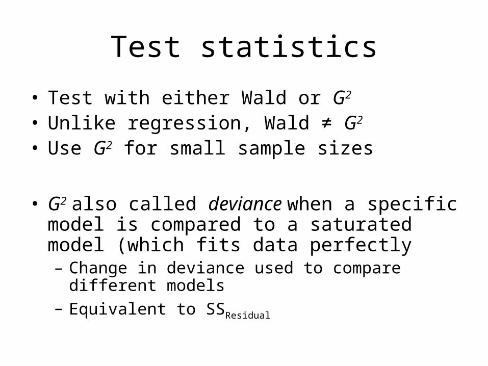
Test statistics

• Test with either Wald or G2

• Unlike regression, Wald ≠ G2

• Use G2 for small sample sizes

• G2 also called deviance when a specific model is compared to a saturated model (which fits data perfectly– Change in deviance used to compare different models– Equivalent to SSResidual

Worked example

Category choices

0 (REFERENCE) 9

1 (RESPONSE) 10

Total : 19

L-L at iteration 1 is -13.170

L-L at iteration 2 is -8.837

L-L at iteration 3 is -7.529

L-L at iteration 4 is -7.138

L-L at iteration 5 is -7.111

L-L at iteration 6 is -7.110

L-L at iteration 7 is -7.110

Log Likelihood: -7.110

Maximum Likelihood estimation, so procedure is iterative: estimate parameters,

calculate log-likelihood. Refine parameter estimates, recalculate log-likelihood.

Continue until convergence:

SYSTAT output:

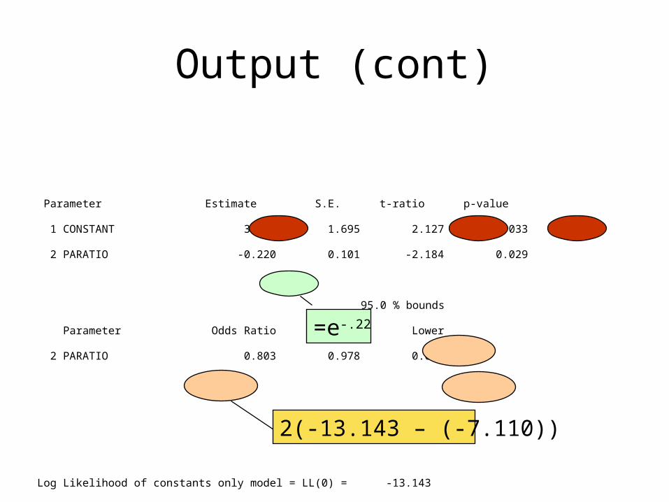
Output (cont)

Parameter Estimate S.E. t-ratio p-value

1 CONSTANT 3.606 1.695 2.127 0.033

2 PARATIO -0.220 0.101 -2.184 0.029

95.0 % bounds

Parameter Odds Ratio Upper Lower

2 PARATIO 0.803 0.978 0.659

Log Likelihood of constants only model = LL(0) = -13.143

2*[LL(N)-LL(0)] = 12.066 with 1 df Chi-sq p-value = 0.001

=e-.22

2(-13.143 – (-7.110))

0 10 20 30 40 50 60 70

P/A ratio

0.0

0.2

0.4

0.6

0.8

1.0

Pre

dict

ed p

roba

bilit

y of

occ

urre

nce

0 10 20 30 40 50 60 70

P/A ratio

0.0

0.2

0.4

0.6

0.8

1.0

Uta

pre

senc

e/ab

senc

e

A special case: toxicity testing

• Logistic regression used to estimate relationship between concentration of substance and response variable

• Equation used to solve for concentration that produces a given level of response– LC50– EC50

Worked example: toxicity testing

• Effect of copper on larvae of a marine invertebrate, Bugula dentata

• Methods– Larvae exposed to copper

at range of concentrations• Range of [Cu] 0 – 400

g/L

– Recorded as swimming or not after 6 hours

– Recorded as live or dead after 24 h

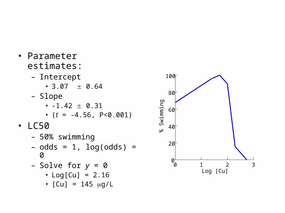
• Parameter estimates:– Intercept

• 3.07 0.64

– Slope• -1.42 0.31 • (t = -4.56, P<0.001)

• LC50– 50% swimming– odds = 1, log(odds) = 0– Solve for y = 0

• Log[Cu] = 2.16• [Cu] = 145 g/L

0 1 2 3Log [Cu]

0

20

40

60

80

100

% S

wim

min

g

0

0 1 2 3

Log [Cu]

0

20

40

60

80

100

% S

wim

min

g

Extension to multiple regression

• Analogous to least squares multiple regression• Generates partial regression coefficients• Test overall regression by comparing fit of

– Full model

– Reduced model (constant or 0 only)

• Wald tests as equivalent to t tests• Use likelihood ratio statistics (deviance)• Assumptions

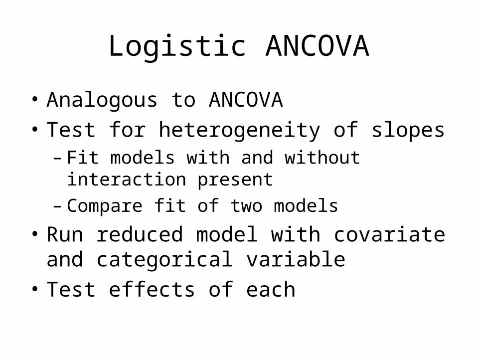
Logistic ANCOVA

• Analogous to ANCOVA

• Test for heterogeneity of slopes– Fit models with and without interaction

present– Compare fit of two models

• Run reduced model with covariate and categorical variable

• Test effects of each

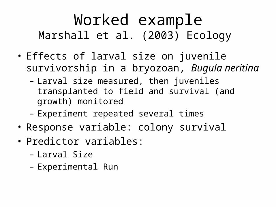
Worked exampleMarshall et al. (2003) Ecology

• Effects of larval size on juvenile survivorship in a bryozoan, Bugula neritina– Larval size measured, then juveniles transplanted to

field and survival (and growth) monitored– Experiment repeated several times

• Response variable: colony survival• Predictor variables:

– Larval Size– Experimental Run

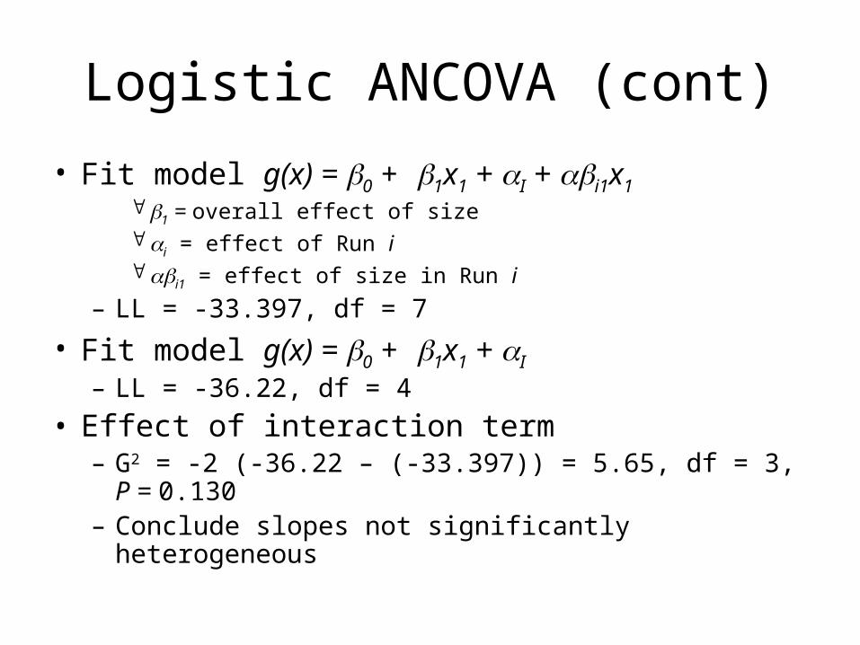
Logistic ANCOVA (cont)

• Fit model g(x) = 0 + 1x1 + I + i1x1 1 = overall effect of size i = effect of Run i i1 = effect of size in Run i

– LL = -33.397, df = 7

• Fit model g(x) = 0 + 1x1 + I

– LL = -36.22, df = 4

• Effect of interaction term– G2 = -2 (-36.22 – (-33.397)) = 5.65, df = 3, P = 0.130– Conclude slopes not significantly heterogeneous

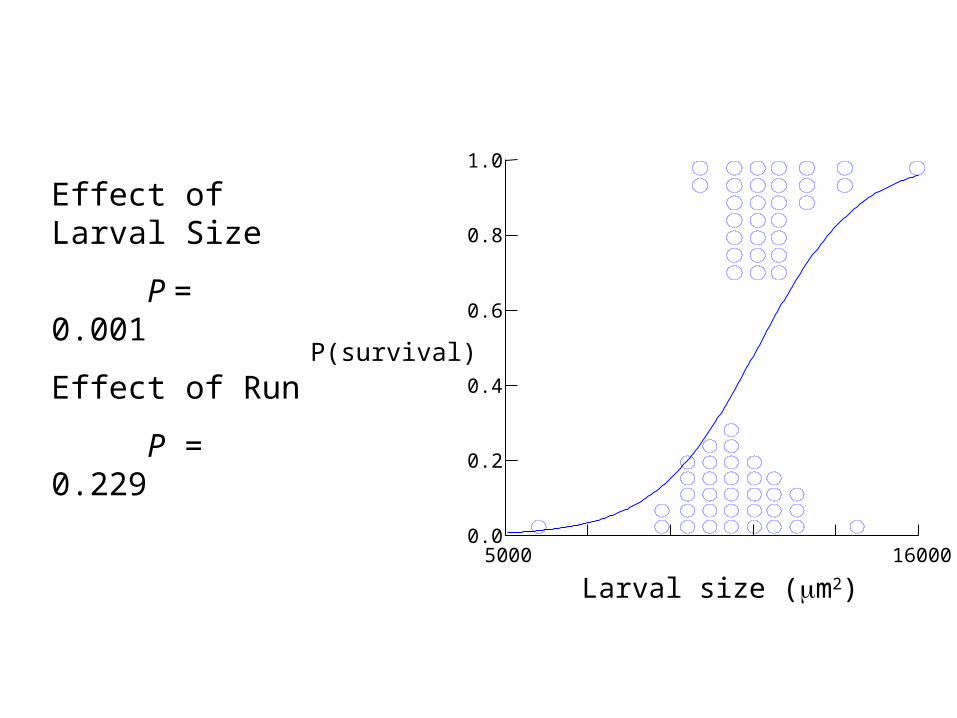
5000 16000

Larval size (m2)

0.0

0.2

0.4

0.6

0.8

1.0

P(survival)

Effect of Larval Size

P = 0.001

Effect of Run

P = 0.229

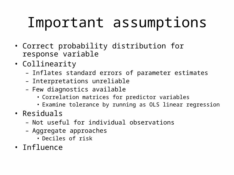
Important assumptions

• Correct probability distribution for response variable• Collinearity

– Inflates standard errors of parameter estimates– Interpretations unreliable– Few diagnostics available

• Correlation matrices for predictor variables• Examine tolerance by running as OLS linear regression

• Residuals– Not useful for individual observations– Aggregate approaches

• Deciles of risk

• Influence

Contingency tables and log-linear models

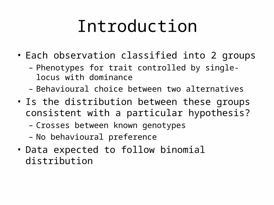
Introduction

• Each observation classified into 2 groups– Phenotypes for trait controlled by single-locus with

dominance– Behavioural choice between two alternatives

• Is the distribution between these groups consistent with a particular hypothesis?– Crosses between known genotypes– No behavioural preference

• Data expected to follow binomial distribution

Binomial test

• Behavioural experiment– n1, n2 are numbers making choices 1 & 2

• Null hypothesis: no preference– p = q = 0.5

• Test– Calculate probability of observing ≥ n1 by

chance– Binomial expansion

• (p + q)n

( ) n n N nNP y n C p q

Example

Binomial Expansion0 1 2 3 4 5 6

0.016 0.094 0.234 0.313 0.234 0.094 0.016

5 animals choose A, 1 chooses B.

One-tailed test: P(5 or more) = P(5) + P(6) = 0.094 + 0.016 = 0.110

Two-tailed test: P(≥ 5 or ≤ 1) = P(5) + P(6) + P(1) +P(0)

= 0.094 + 0.016 + 0.094 + 0.016

= 0.220

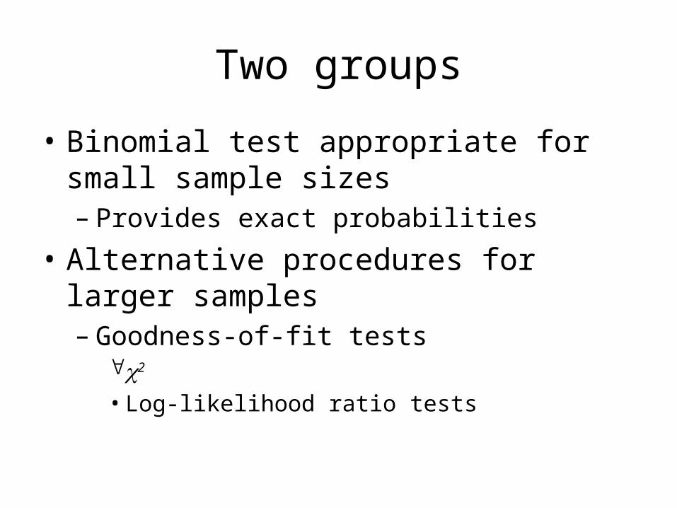
Two groups

• Binomial test appropriate for small sample sizes– Provides exact probabilities

• Alternative procedures for larger samples– Goodness-of-fit tests

2

• Log-likelihood ratio tests

2

1

( )Ki i

i i

o e

e

2 Goodness of fit test

• Data in K groups

• oi is observed number in group i

• ei is expected number in group I

• Assess using 2 with k-1 df

More groups

• Outcome no longer binomial, but multinomial:(p1 + p2 + … pi + … pk)n

• Computationally difficult

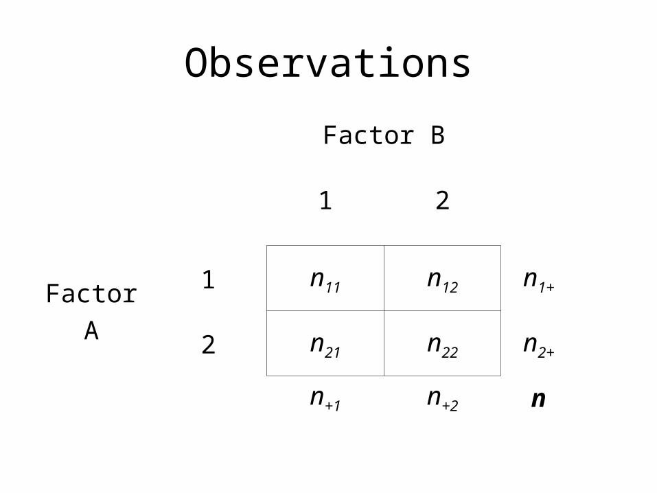
Observations

Factor B

1 2

Factor

A

1 n11 n12 n1+

2 n21 n22 n2+

n+1 n+2 n

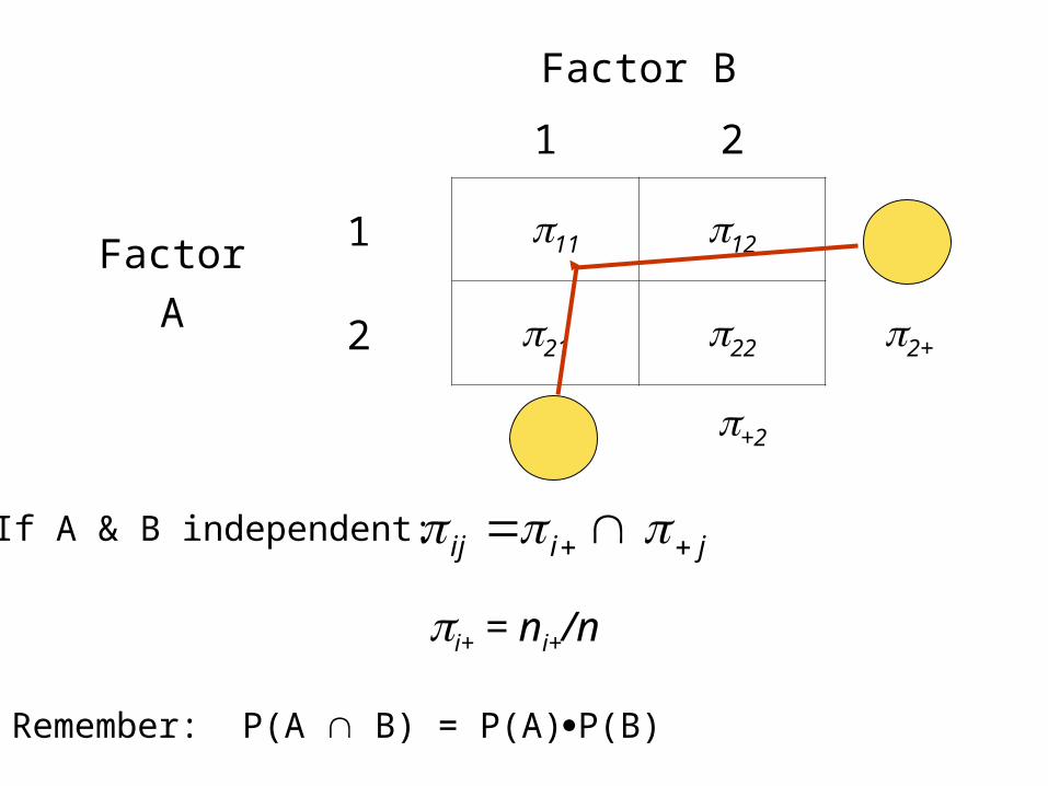
Factor B

1 2

Factor

A

1 11 12 1+

2 21 22 2+

+1 +2

i+ = ni+/n

ij i j If A & B independent:

Remember: P(A B) = P(A)P(B)

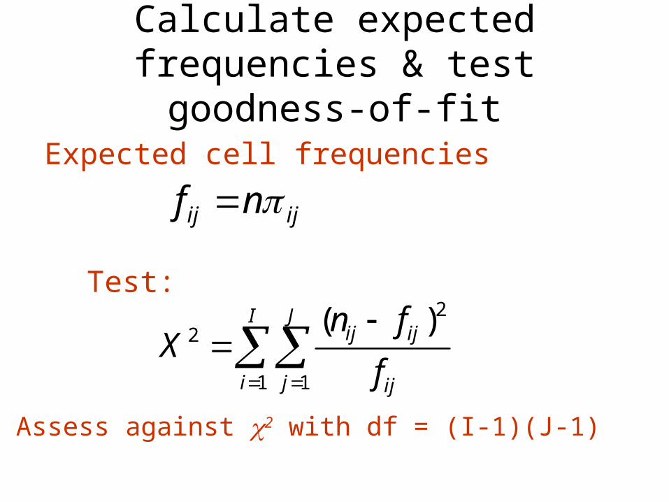
Calculate expected frequencies & test goodness-of-fit

f nij ij

22

1 1

( )I Jij ij

i j ij

n fX

f

Test:

Assess against 2 with df = (I-1)(J-1)

Expected cell frequencies

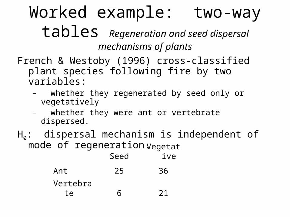
Worked example: two-way tables Regeneration and seed dispersal mechanisms of plants

French & Westoby (1996) cross-classified plant species following fire by two variables: – whether they regenerated by seed only or vegetatively – whether they were ant or vertebrate dispersed.

H0: dispersal mechanism is independent of mode of regeneration.

Seed Vegetative

Ant 25 36

Vertebrate 6 21

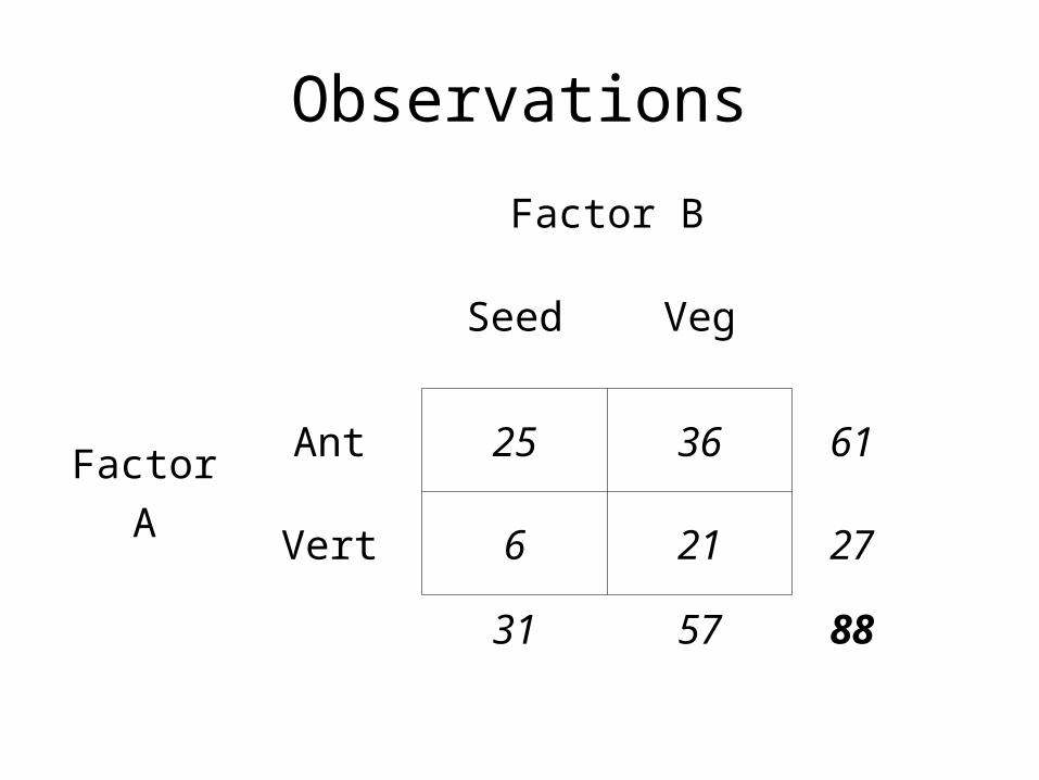
Observations

Factor B

Seed Veg

Factor

A

Ant 25 36 61

Vert 6 21 27

31 57 88

Expected values

25 36 61

6 21 27

31 57 88

21.5 39.5 0.69

9.5 17.5 0.31

0.35 0.65

(25-21.5)2 / 21.5 = 0.57

2 = 2.89, df = 1, P = 0.089

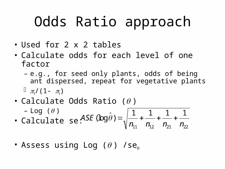
Odds Ratio approach

• Used for 2 x 2 tables• Calculate odds for each level of one factor

– e.g., for seed only plants, odds of being ant dispersed, repeat for vegetative plants

i/(1- i)

• Calculate Odds Ratio ( )– Log ( )

• Calculate se:

• Assess using Log ( ) /se

ASEn n n n

(log ) 1 1 1 1

11 12 21 22

Example: odds ratio test

25 36 61

6 21 27

31 57 88

0.81 0.63

0.19 0.37

4.17 1.71 Odds

4.17 / 1.71 = 2.43 = 0.89

se = 0.53

95% CI = 0.86 to 6.89

Small Sample Sizes

• Aim for expected values <5 in no more than 20% of cells– Pool categories to raise expected numbers

• Yate’s correction– Adjustment for continuity– Not widely recommended now

• Fisher’s exact test– For 2 x 2 tables

• Other exact methods– Randomisation tests

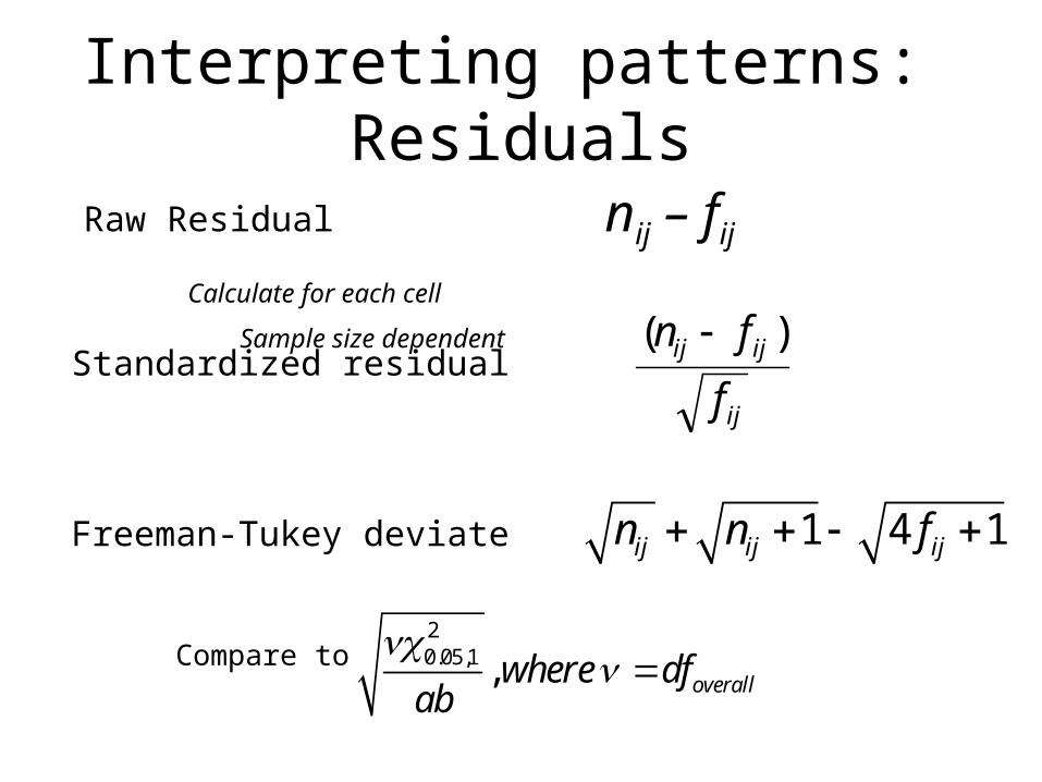
Interpreting patterns: Residuals

Raw Residual nij – fij

Calculate for each cell

Sample size dependent ( )n f

fij ij

ij

Standardized residual

1 4 1ij ij ijn n f

20.05,1 , overallwhere dfab

Freeman-Tukey deviate

Compare to

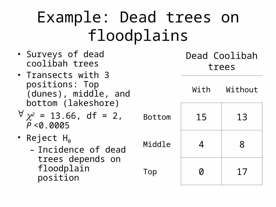
Example: Dead trees on floodplains

• Surveys of dead coolibah trees

• Transects with 3 positions: Top (dunes), middle, and bottom (lakeshore)

2 = 13.66, df = 2, P <0.0005

• Reject H0

– Incidence of dead trees depends on floodplain position

Dead Coolibah trees

With Without

Bottom 15 13

Middle 4 8

Top 0 17

Dead Coolibah trees

With Without

Bottom 1.855 -1.312

Middle 0.000 0.000

Top -2.380 1.683

Example: Dead trees on floodplains

• Standardized residuals

• More dead than expected near bottom, fewer than expected on dunes

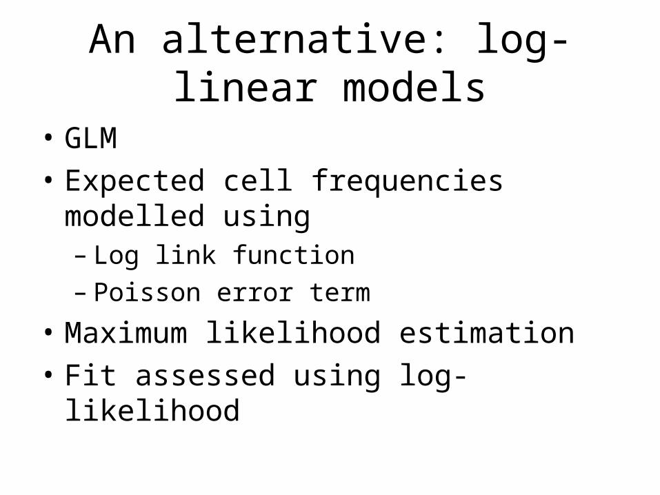
An alternative: log-linear models

• GLM

• Expected cell frequencies modelled using– Log link function– Poisson error term

• Maximum likelihood estimation

• Fit assessed using log-likelihood

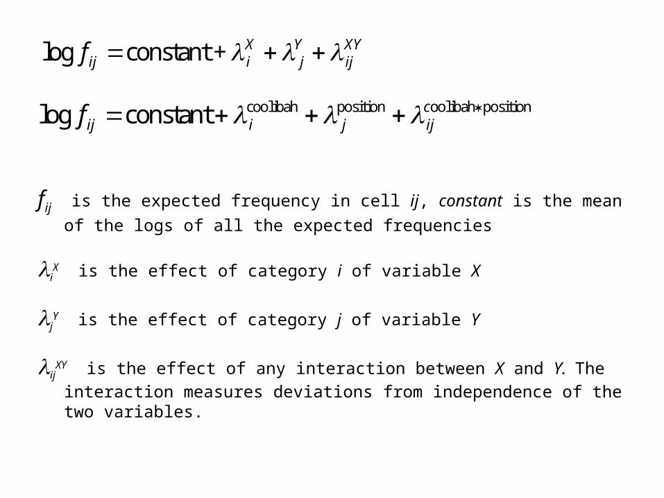
log f ij iX

jY

ijXY constant +

log f ij i j ijc constant coolibah position oolibah position

fij is the expected frequency in cell ij, constant is the mean of the logs of all the

expected frequencies

iX is the effect of category i of variable X

jY is the effect of category j of variable Y

ijXY is the effect of any interaction between X and Y. The interaction measures

deviations from independence of the two variables.

log f ij iX

jY

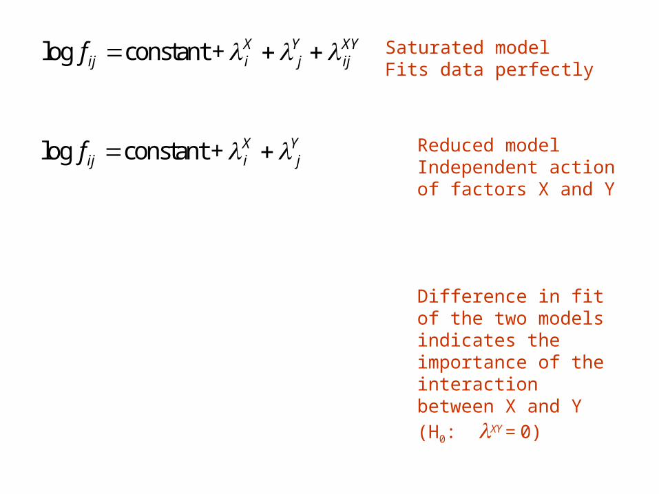
ijXY constant + Saturated model

Fits data perfectly

log f ij iX

jY constant + Reduced model

Independent action of factors X and Y

Difference in fit of the two models indicates the importance of the interaction between X

and Y (H0: XY = 0)

For coolibah example

log f ij i j ijc constant coolibah position oolibah position

log f ij i j constant coolibah position

Log-likelihood

-10.429, df = 3

-19.735, df = 2

G2 = -2(LLmodel – LLsaturated)

= -2(-19.735 – (-10.429))

= 18.61, df = 1, P < 0.001

Reject H0

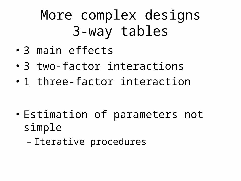
More complex designs3-way tables

• 3 main effects

• 3 two-factor interactions

• 1 three-factor interaction

• Estimation of parameters not simple– Iterative procedures

log f ijk iX

jY

kZ

ijXY

ikXZ

jkYZ

ijkXYZ constant

Full model:

Loglinear model df

X + Y + Z IJK-I-J-K+2

X + Y + Z + XY (K-1)(IJ-1)

X + Y + Z + XZ (J-1)(IK-1)

X + Y + Z + YZ (I-1)(JK-1)

X + Y + Z + XZ + YZ K(I-1)(J-1)

X + Y + Z + XY + YZ J(I-1)(K-1)

X + Y + Z + XY + XZ I(J-1)(K-1)

X + Y + Z + XY + XZ + YZ (I-1)(J-1)(K-1)

Saturated model:X + Y + Z + XY + XZ + YZ + XYZ

0

Models are hierarchical:Higher order term “forces” all simpler terms inOmission of two-way term forces omission of 3-way

Representative models

Comparison of models

• Choosing best model– Lowest value of G2

– Akaike Information Criterion (AIC)• Adjusts for number of parameters in model

• G2 – 2 dftest of model

• Tests of hypothesis– Contrast fit of two models differing in the

presence of the term in question

Worked exampleWildebeeste carcasses (Sinclair & Arcese 1995)

• Carcasses classified according to– Sex

– Cause of death • (predation or not)

– Health (state of bone marrow)

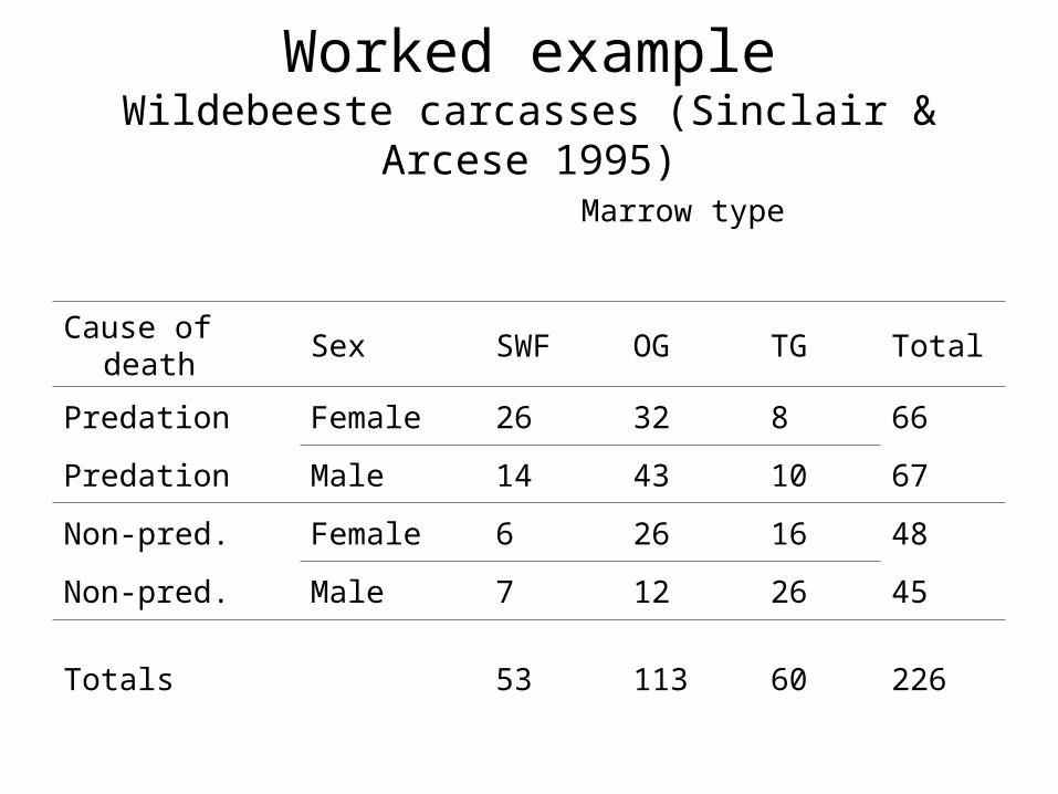
Worked exampleWildebeeste carcasses (Sinclair & Arcese 1995)

Marrow type

Cause of death Sex SWF OG TG Total

Predation Female 26 32 8 66

Predation Male 14 43 10 67

Non-pred. Female 6 26 16 48

Non-pred. Male 7 12 26 45

Totals 53 113 60 226

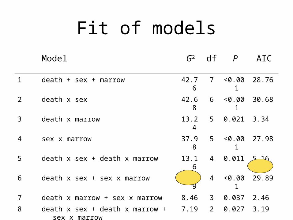
Fit of models

Model G2 df P AIC

1 death + sex + marrow 42.76 7 <0.001 28.76

2 death x sex 42.68 6 <0.001 30.68

3 death x marrow 13.24 5 0.021 3.34

4 sex x marrow 37.98 5 <0.001 27.98

5 death x sex + death x marrow 13.16 4 0.011 5.16

6 death x sex + sex x marrow 37.89 4 <0.001 29.89

7 death x marrow + sex x marrow 8.46 3 0.037 2.46

8 death x sex + death x marrow + sex x marrow 7.19 2 0.027 3.19

9 Saturated (full) model 0 0

Tests of hypotheses1 death + sex + marrow 42.76 7

2 death x sex 42.68 6

3 death x marrow 13.24 5

4 sex x marrow 37.98 5

5 death x sex + death x marrow 13.16 4

6 death x sex + sex x marrow 37.89 4

7 death x marrow + sex x marrow 8.46 3

8 death x sex + death x marrow + sex x marrow 7.19 2

9 Saturated (full) model 0 0