on the interior regularity of weak … e-publica˘coes do departamento de matem atica universidade...

Pre-Publicacoes do Departamento de MatematicaUniversidade de CoimbraPreprint Number 16–18

ON THE INTERIOR REGULARITY OF WEAK SOLUTIONSTO THE 2-D INCOMPRESSIBLE EULER EQUATIONS

JUHANA SILJANDER AND JOSE MIGUEL URBANO

Abstract: We consider the 2-D incompressible Euler equations in a bounded do-main and show that local weak solutions are exponentially integrable, uniformly intime, under minimal integrability conditions. This is a Serrin-type interior regular-ity result

u ∈ L2+εloc (ΩT ) =⇒ regularity

for weak solutions in the energy space L∞t L

2x satisfying appropriate vorticity esti-

mates. The argument is completely local in nature as the result follows from thestructural properties of the equation alone, while completely avoiding all sorts ofboundary conditions and related gradient estimates. To the best of our knowledge,the approach we follow is new in the context of Euler equations and provides analternative look at interior regularity issues. We also show how our method can beused to give a modified proof of the classical Serrin condition for the regularity ofthe Navier-Stokes equations in any dimension.

Keywords: Incompressible Euler and Navier-Stokes system, Moser iteration, Biot-Savart law, local regularity.

AMS Subject Classification (2010): Primary 35Q31. Secondary 76B03, 35B65,35Q30.

1. IntroductionIn this paper, we consider local weak solutions u ∈ L2

loc(ΩT ) of the incom-pressible Euler equations in two space dimensions

∂tu+ (u · ∇)u+∇p = 0 and div u = 0, (1.1)

and show, under appropriate integrability conditions on u and its vorticityω, they are exponentially integrable uniformly in time.

Received April 22, 2016.J.S. was supported by the Academy of Finland grant 259363 and by a Vaisala Foundation travel

grant. J.M.U. was partially supported by the Centre for Mathematics of the University of Coimbra– UID/MAT/00324/2013, funded by the Portuguese Government through FCT/MCTES and co-funded by the European Regional Development Fund through the Partnership Agreement PT2020.This work initiated while the authors were visiting the Mittag-Leffler Institute during the program”Evolutionary Problems” and was concluded while J.S. visited the University of Coimbra; we thankboth institutions for the kind hospitality.

1

2 J. SILJANDER AND J.M. URBANO

Despite their physical relevance, for instance in the context of Kolmogorov’stheory of turbulence, much of what we know about the weak solutions of (1.1)concerns some sort of pathological behaviour. For example, weak solutionsare not unique: Scheffer constructed in [21] a two-dimensional weak solutionwhich is compactly supported in space and time; a simpler counter-examplewas provided later by Shnirelman [23]. More recently, De Lellis and Szeke-lyhidi Jr. [8] have shown that even locally bounded weak solutions may failto be unique. Another line of research deals with Onsager’s conjecture thatthe critical exponent for Holder continuous weak solutions to dissipate en-ergy is 1

3 . The current threshold exponent for anomalous dissipation is 15 (see

[14, 4]) and the fact that any C0, 13 weak solution conserves energy was provenby Constantin, E and Titi in [6]. For more on Euler equations we refer to thebook of Majda and Bertozzi [19], and the expository articles by Constantin[5] or Bardos and Titi [2]. Recent interesting papers in two dimensions are[15, 16].

Instead of studying pathological behaviour, we aim here at establishinga regularity result. In the whole space R2, or in a bounded domain withthe Neumann boundary condition u · ν = 0, it is well known that sufficientintegrability of the vorticity ω implies the gradient estimate

u, ω ∈ L∞t L2x =⇒ u ∈ L∞t H1

x. (1.2)

By Poincare inequality, one immediately obtains that u ∈ L∞t BMOx, whichis also known to be optimal by explicit solution formulas. Our contribu-tion is in showing that almost the same optimal regularity can be obtained,by purely local arguments, merely from the structural properties of equa-tions (1.1).

More precisely, we work in a domain Ω ⊂ R2, without any sort of boundaryconditions, and prove the exponential integrability of the velocity, uniformlyin time, under minimal integrability assumptions. Our main result is a Serrin-type [22] interior regularity theorem

u ∈ L2+εloc (ΩT ) =⇒ regularity

for weak solutions in the energy space L∞t L2x. In particular, we do not make

any kind of assumptions on initial data.In the proof we study the vorticity formulation of the Euler equations. In

order to make sense of weak solutions, we assume ω ∈ L2loc(ΩT ) and exploit

the corresponding energy estimates for the vorticity. We then combine these

ON THE INTERIOR REGULARITY OF THE 2-D EULER EQUATIONS 3

vorticity estimates with the Hardy-Littlewood-Sobolev theorem on fractionalintegration, and apply a Biot-Savart type potential estimate to improve theintegrability of the velocity field in a Moser iteration procedure, to obtainthe main result. Our reasoning, in a nutshell, is that a proper modification ofthe Moser local regularity machinery (see [20]) can still be applied completelywithout gradient estimates, such as (1.2), if we have a suitable Biot-Savarttype result at our disposal.

The same approach naturally applies to the Navier-Stokes system and wegive a modified proof of the classical Serrin regularity condition [22] througha Moser iteration technique where, contrary to the original argument of Ser-rin, we first prove u ∈ L∞t L

px, for a large enough p, and only then show

the boundedness of the vorticity ω. While this machinery is probably well-known to the experts, the argument is still somewhat delicate and all thedetails we provide are scattered and difficult to find in the literature. Inter-estingly enough, we manage to improve the original Serrin result in the twodimensional setting.

2. Preliminaries and main result2.1. Notation. We denote by Br(xo) the standard open ball in Rd, withradius r > 0 and centre at xo. Let Ω be an open set in Rd and denote the

space-time cylinder ΩTdef= Ω × (0, T ]. For the boundary of the set we use

the standard notation ∂Ω. We define the parabolic boundary of a space-timecylinder as

∂pΩTdef=(∂Ω× [0, T ]

)∪(Ω× 0

)and denote dµ

def= dx dt.

As we will only consider interior regularity results, it is enough to considerlocal space-time cylinders Br(xo)×(to−r, to). By translation, we may alwaysassume xo = to = 0. For such cylinder, we will use the notation

Qr = Br × Irdef= Br(0)× (−r, 0),

for r > 0. For the integral average, we write

−∫

Ω

|u| dx def=

1

|Ω|

∫Ω

|u| dx.


The corresponding averaged Lq-norm will be denoted by

‖u‖Lq(Ω),avgdef=

(−∫

Ω

|u|q dx) 1

q

,

for q > 0. For γ > 0, we define the class of exponentially integrable functionsu ∈ exp

(γ√L(Ω)

)by requiring∫

Ω

eγ√|u(x)| dx <∞.

The corresponding local space is defined by requiring the finiteness of thisintegral for all compact sets K b Ω.

2.2. Definitions. We now make precise the concept of weak solution we willbe using.

Definition 2.1. We say a vector field u ∈ L2loc(ΩT ) is a weak solution of

equation (1.1) in ΩT if ∫Ω

u(x, t) · ∇ψ(x) dx = 0,

for every ψ ∈ H10(Ω) and almost every t ∈ [0, T ], and if∫ T

0

∫Ω

u · ∂tφ+d∑i=1

ui(u · ∇)φi dx dt = 0, (2.1)

for every smooth test function φ with compact support in space-time such that∇ · φ = 0.

Let us now restrict to the two-dimensional setting and introduce the vor-ticity

ωdef= curlu = ∂x1u2 − ∂x2u1.

It is an easy exercise to show that if u is a weak solution of equation (1.1) inΩT and ω ∈ L2

loc(ΩT ), then the vorticity equation

∂tω + (u · ∇)ω = 0

holds in the weak sense. We will exploit in the sequel energy estimates forthis equation, which we formalize into the following definition.


Definition 2.2. Let Ω ⊂ R2 and u be a weak solution of equation (1.1) inΩT . We say that u satisfies the vorticity estimates if ω ∈ L2

loc(ΩT ) and thereexists a constant Vo > 0 such that

esssup0≤t≤T

∫Ω

|ω|1+αζ(x, t) dx

≤ Vo

∫ T

0

∫Ω

|ω|1+α[|u||∇ζ|+ |∂tζ|

]dµ,

(VE)

for every α ∈ [0, 1), and for every non-negative test function ζ ∈ C∞(ΩT )that vanishes in a neighbourhood of the parabolic boundary ∂pΩT .

Remark 2.1. A rigorous treatment of the vorticity estimates would typicallyrequire an approximation scheme, for example in the spirit of the celebratedDiPerna-Lions theory [9]. Strictly speaking, this requires the vorticity to beat least in L∞t L

2x, which is stronger than we assume. This notwithstand-

ing, subsequent results by Ambrosio [1] and Bouchut-Crippa [3] brought theintegrability threshold closer to ours.

The focus in this paper is not in deriving these a priori estimates but ratherin showing that, once they hold, interior regularity can be obtained underminimal integrability assumptions. The underlying reasoning parallels theuse of De Giorgi classes in the context of regularity theory for second-orderelliptic and parabolic equations [7, 12]; see also [26] for an application to theNavier-Stokes system.

2.3. The main result. Our main theorem is an exponential integrabilityresult implying that the velocity field u of the incompressible Euler systemcannot form singularities too fast if it is – a priori – sufficiently integrabletogether with its vorticity. This is a Serrin-type [22] interior regularity resultyielding, for weak solutions u ∈ L∞t L2

x satisfying (VE),

u ∈ L2+εloc (ΩT ) =⇒ regularity.

In other words, if a weak solution blows up then either our integrabilityassumptions must be violated or the blow-up can only be, roughly speaking,of logarithmic type.

Theorem 2.1. Let u ∈ L∞loc(0, T ;L2loc(Ω)) be a weak solution of equation (1.1)

in two dimensions satisfying the vorticity estimates (VE). Then, if u ∈


L2+εloc (ΩT ) for some ε > 0, there exists a constant C = C(ε, Vo) > 0 such that

for every Q4r = B4r × I4r b ΩT we have

u ∈ L∞(Ir; exp(γ√L(Br)

)),

where

γdef= C

[(r2−∫Q4r

|ω|2 dµ+ 1

) 12(−∫Q4r

|u|2+ε dµ+ 1

) 12+ε

+ ‖u‖L∞(I4r;L1(B4r),avg)

].

Remark 2.2. If Ω = R2, or in the case of the Neumann boundary conditionu · ν = 0, the DiPerna-Lions borderline assumption is known to be equivalentto u ∈ L∞t H1

x, provided u belongs to the energy space L∞t L2x. In particular,

we have

u, ω ∈ L∞t L2x =⇒ u ∈ L∞t H1

x (2.2)

and obtain immediately, from the Poincare inequality, that u ∈ L∞t BMOx.This is also known to be optimal due to an explicit stationary solution ob-tained via

u(x) =(−x2

r2,x1

r2

)T∫ r

0

sω(s) ds, r = |x|,

with the radial vorticity

ω(s) =1

s log 1s

.

For details we refer to [19, Section 2.2.1].We work in the interior and our results are local in the sense that we do not

use any sort of boundary (or initial) information, which is crucial in the abovereasoning. Our contribution is thus in showing that one is still able to obtainthe almost optimal interior integrability estimate u ∈ L∞t exp(γ

√Lx) merely

from the structural properties of equation (1.1), while completely avoidingboundary conditions and the heavy machinery of gradient estimates suchas (2.2). Finally, while we have stated the theorem with the standard en-ergy space L∞t L

2x, our proof actually works with merely u ∈ L∞t L1

x.

The proof uses a Moser iteration technique, with the Sobolev embeddingreplaced by the Hardy-Littlewood-Sobolev theorem on fractional integration.This provides the required bound for the Biot-Savart potential, which is thenused to improve the integrability of u. We iterate the obtained estimates todeduce a quantitative growth rate for the spatial Lp-norm of u, uniformly in


time. This enables us to show that the norms are exponentially summable,and we conclude the result.

In the case of the Navier-Stokes system, where we have additional controlon the gradient, we may use our method to give a modified proof of the clas-sical Serrin regularity condition. Moreover, we can relax the Serrin conditionin two dimensions to assume merely u ∈ Lq for q > 2 instead of the Serrincondition which, more or less, assumes q > 4.

2.4. Auxiliary tools. Although we do not employ the Sobolev embeddingin our arguments for the Euler equations, we will use it in the very end whenstudying the Navier-Stokes system. Even there, we only use it as a formaltool, whereas the rigorous argument is conducted for suitable mollificationssuch that no existence of Sobolev gradients is required. We recall that ford ≥ 2 and for u ∈ H1

0(Ω), by the Sobolev embedding, there exists a constantC = C(d) > 0 such that(

−∫

Ω

|u|2∗ dx) 1

2∗

≤ Cdiam(Ω)

(−∫

Ω

|∇u|2 dx) 1

2

,

where

2∗def=

any number in (2,∞), for d = 22dd−2 , for d ≥ 3.

An easy consequence of the above result is a parabolic Sobolev embedding foru ∈ L∞(0, T ;L2(Ω)) ∩ L2(0, T ;H1

0(Ω)). In this case, there exists a constantC = C(d) > 0 such that(∫ T

0

(−∫

Ω

|u|q dx) s

q

dt

) 1s

≤ Cdiam(Ω)2s

(esssup0≤t≤T−

∫Ω

|u|2 dx+

∫ T

0

−∫

Ω

|∇u|2 dµ) 1

2

,

(2.3)

for any 2 < q, s <∞ satisfying

d

q+

2

s=d

2.


Next we turn to a Hardy-Littlewood-Sobolev lemma on fractional integra-tion. We recall the definition of the Riesz potential

(Iβf)(x) = (−∆)−β2 f(x) = cβ

∫Rd

f(y)

|x− y|d−βdy,

with 0 < β < d, which arises naturally via the Biot-Savart law. Here the vor-ticity ω plays the role of f and we have for the velocity field |u| ≤ C|(I1ω)(x)|(cf. Lemma 3.1). We will however work in a ball rather than the whole spaceand for this reason we will always consider all locally defined functions as be-ing extended as zero outside the local set to make sense of the above non-localintegral. With this convention in mind, we have the following well-knownlemma.

Lemma 2.1. Let 0 < β < d and f ∈ Lq(Rd) for 1 < q < d/β. Then thereexists a constant C = C(d, β, q) > 0 such that

‖Iβf‖Ls(Rd) ≤ C‖f‖Lq(Rd),for

s =dq

d− βqand

C(d, β, q) ≤ C(d, β) max

(q − 1)−(1−βd), s1−βd.

For the proof see [24, Chapter V, §1.3].

3. A local Biot-Savart estimateIn this section we establish a version of the local Biot-Savart law for

solenoidal vector fields. Observe that, under our assumptions, the error termbelow is a constant, bounded both in space and time, unlike what happensin the classical paper of Serrin [22, Lemma 2], where the error is known to bemerely a harmonic function in space. In order to obtain the uniform boundin time, we need to use the assumption that u is a weak solution and locallyin L∞t L

1x ∩ L2+ε

t,x . In particular, it does not seem to be enough to assume ubeing solenoidal.

Let σ > 0. In order to simplify the notation we will denote

σQdef= Qσr

as well as

σIdef= Iσr and σB

def= Bσr.


In the same spirit, for σ = 1, we denote Qdef= Qr, B

def= Br and I

def= Ir.

Lemma 3.1. Let ε > 0, k ∈ R2 and 0 < σ < 1. Suppose u is a weak solutionto equation (1.1) in ΩT c 2Q satisfying (VE) such that u ∈ L2+ε(2Q). Thenthere exists a constant C = C(ε, Vo) > 0 such that for every (x, t) ∈ σQ wehave

|u(x, t)− k| ≤ 1

2π

∫B

|ω(y, t)||x− y|

dy +C

(1− σ)3

[‖u(·, t)− k‖L1(B),avg + Γ

],

where

Γ = Γ(2Q)def= 2r

(−∫

2Q

|ω|2 dµ) 1

2(−∫

2Q

|u|2+ε + 1 dµ

) 12+ε

. (3.1)

Remark 3.1. Observe that the term ‖u(·, t) − k‖L1(B),avg is, a priori, well-defined only for almost every t ∈ 2I. In case this quantity is not well-defined,we interpret the value being infinite, and the estimate holds trivially.

Proof : By translation, we may assume Q to be centred at the origin, asalready suggested by the slight abuse of notation in the statement of thelemma. Since div u = 0 in Ω, there exists a stream function ϕ(x, t) such that

u1 = −∂x2ϕ and u2 = ∂x1ϕ. (3.2)

Observe that ω = curlu = ∆ϕ in Ω c B. Recalling that the Green functionfor the Laplacian in the ball Br(0) ⊂ R2 is given by

G(x, y) =1

2π

[ln

(|x|r

∣∣∣∣y − x

|x|2r2

∣∣∣∣)− ln |x− y|],

we have

ϕ(x, t) = −∫∂Br(0)

∂G(x, y)

∂yνϕ(y, t) dH1(y)−

∫Br(0)

G(x, y)ω(y, t) dy

def= J1(x, t) + J2(x, t).

(3.3)


Here H1 denotes the one-dimensional Hausdorff measure on ∂Br(0). A te-dious but straightforward calculation shows for x, y ∈ Br(0) that

∂xiG(x, y) = − 1

2π

xi − yi|x− y|2−|y|(|y|xi − yi

|y|r2)

∣∣∣|y|x− y|y|r

2∣∣∣2

≤ − 1

2π

xi − yi|x− y|2

− |y|∣∣∣|y|x− y|y|r

2∣∣∣

≤ − 1

2π

[xi − yi|x− y|2

− 1

r − |x|

].

Therefore, we obtain

|∂xiJ2(x, t)| ≤1

2π

∫B

[1

|x− y|+

1

r − |x|

]|ω(y, t)| dy.

We choose a test function ζ ∈ C∞(2Q) such that ζ = 1 in Q, ζ = 0 on∂p(2Q) and satisfies the bounds

|∇ζ| ≤ Cr−1 and

∣∣∣∣∂ζ∂t∣∣∣∣ ≤ Cr−1.

We apply the vorticity estimates (VE) with α = 0 and Holder’s inequalityto obtain

esssupt∈I

∫B

|ω(y, t)| dy ≤ Cr−1

∫2Q

|ω||u|+ |ω| dµ

≤ Cr−1

(∫2Q

|ω|2 dµ) 1

2(∫

2Q

(|u|+ 1)2 dµ

) 12

,

(3.4)

and, therefore, we may conclude that

esssupσB

∫B

|ω(y, t)|r − |x|

dy ≤ 1

(1− σ)resssupt∈I

∫B

|ω(y, t)| dy

≤ C

(1− σ)r2

(∫2Q

|ω|2 dµ) 1

2(∫

2Q

(|u|+ 1)2 dµ

) 12

≤ Cr

(1− σ)

(−∫

2Q

|ω|2 dµ) 1

2(−∫

2Q

|u|2+ε dµ+ 1

) 12(1+ε)

,


uniformly for almost every t ∈ I.

Let ldef= (−k1, k2). We have shown that

∂xiϕ(x, t)− lj = [∂xiJ1(x, t)− lj] + ∂xiJ2(x, t), i = 1, 2, i 6= j, (3.5)

where

esssupσB|∂xiJ2(x, t)| ≤1

2π

∫B

|ω(y, t)||x− y|

dy +CΓ

1− σ, (3.6)

for a constant C independent of the time variable t.It remains to show a similar estimate for ∂xiJ1(x, t) − lj. We begin by

observing that, for each t, this is a harmonic function in the space variables.Therefore, using the L∞−L1 estimate for harmonic functions, the represen-tation (3.5) and (3.6), as well as Jensen’s inequality, give

esssupσB|∂xiJ1(·, t)− lj|

≤ C

(1− σ)2−∫

1+σ2 B

|∂xiJ1(x, t)− lj| dx

≤ C

(1− σ)2−∫

1+σ2 B

|∂xiϕ(x, t)− lj| dx+C

(1− σ)2−∫

1+σ2 B

|∂xiJ2(x, t)| dx

≤ C

(1− σ)2−∫B

|u(x, t)− k| dx+CΓ

(1− σ)3

+C

(1− σ)2

(−∫B

(∫B

|ω(y, t)||x− y|

dy

)2(1+ε)

dx

) 12(1+ε)

,

(3.7)

for almost every t ∈ I. Now, by the Hardy-Littlewood-Sobolev estimate ofLemma 2.1 and by the vorticity estimates (VE), with α = 2 − 2

2+ε − 1, weobtain that

esssupt∈I

∥∥∥∥∫B

|ω(y, t)|| · −y|

dy

∥∥∥∥L2(1+ε)(B),avg

≤ C(ε) resssupt∈I‖ω(·, t)‖L2− 2

2+ε (B),avg

≤ Cr

(−∫

2Q

|ω|2 dµ) 1

2(−∫

2Q

|u|2+ε dµ+ 1

) 12(1+ε)

.


Combining the above estimates yields

esssupσB|∂xiJ1(·, t)− lj|

≤ Cr

(1− σ)3

(−∫

2Q

|ω|2 dµ)1/2(

−∫

2Q

|u|2+ε + 1 dµ

) 12(1+ε)

+C‖u(·, t)− k‖L1(B),avg

(1− σ)2,

as required. This, together with (3.5), (3.6) and (3.2) concludes the proof.

As a simple corollary of the previous lemma we obtain the following esti-mate.

Corollary 3.1. Let 0 < σ < 1. Suppose u is a weak solution to equation (1.1)in ΩT c 2Q satisfying (VE) such that u ∈ L2+ε(2Q), for some ε > 0. Thenthere exists a constant C = C(ε, Vo) > 0 such that for every (x, t) ∈ σQ wehave

|u(x, t)− u2B| ≤1

2π

∫B

|ω(y, t)||x− y|

dy +C

(1− σ)3

[‖u(·, t)− u2B‖L1(2B),avg + Γ

],

where Γ is as in (3.1). In particular, the constant C is independent of thetime variable t.

Proof : Choose k =((u1)2B, (u2)2B

)in Lemma 3.1.

We will next use the above Biot-Savart law in place of a Sobolev embeddingin a suitable Moser iteration scheme. This allows us to iteratively improvethe integrability of the velocity field u. Observe that we only require someintegrability of ω rather than the existence of full Sobolev gradients.

4. Uniform integrability estimates for the weak solutionsIn this section we will prove Theorem 2.1. The main steps of the proof are

as follows:

1. use the vorticity estimates (VE) to obtain an Lq estimate for ω uni-formly in time, where on the right hand side the integrability assump-tions on u and ω are used to control the different terms;

2. combine this uniform in time Lq estimate with the Hardy-Littlewood-Sobolev estimate of Lemma 2.1 and the Biot-Savart type estimate ofLemma 3.1 to obtain that u ∈ L2+ρ, for some quantitatively deter-minable ρ > ε;


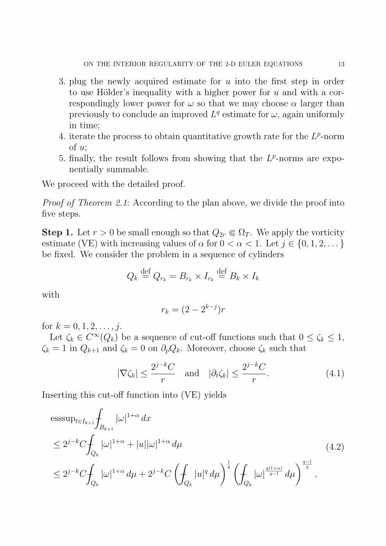
3. plug the newly acquired estimate for u into the first step in orderto use Holder’s inequality with a higher power for u and with a cor-respondingly lower power for ω so that we may choose α larger thanpreviously to conclude an improved Lq estimate for ω, again uniformlyin time;

4. iterate the process to obtain quantitative growth rate for the Lp-normof u;

5. finally, the result follows from showing that the Lp-norms are expo-nentially summable.

We proceed with the detailed proof.

Proof of Theorem 2.1: According to the plan above, we divide the proof intofive steps.

Step 1. Let r > 0 be small enough so that Q2r b ΩT . We apply the vorticityestimate (VE) with increasing values of α for 0 < α < 1. Let j ∈ 0, 1, 2, . . . be fixed. We consider the problem in a sequence of cylinders

Qkdef= Qrk = Brk × Irk

def= Bk × Ik

with

rk = (2− 2k−j)r

for k = 0, 1, 2, . . . , j.Let ζk ∈ C∞(Qk) be a sequence of cut-off functions such that 0 ≤ ζk ≤ 1,

ζk = 1 in Qk+1 and ζk = 0 on ∂pQk. Moreover, choose ζk such that

|∇ζk| ≤2j−kC

rand |∂tζk| ≤

2j−kC

r. (4.1)

Inserting this cut-off function into (VE) yields

esssupt∈Ik+1−∫Bk+1

|ω|1+α dx

≤ 2j−kC−∫Qk

|ω|1+α + |u||ω|1+α dµ

≤ 2j−kC−∫Qk

|ω|1+α dµ+ 2j−kC

(−∫Qk

|u|q dµ) 1

q(−∫Qk

|ω|q(1+α)q−1 dµ

) q−1q

,

(4.2)


for 2 < q ≤ ∞ and for a uniform constant C. For each q ∈ (2,∞], we chooseα ∈ (0, 1] such that

q(1 + α)

q − 1= 2.

This choice yields α = 1− 2/q ∈ (0, 1), and we obtain from (4.2) that

esssupt∈Ik+1−∫Bk+1

|ω|2(1− 1q) dx

≤ 2j−kC

(−∫Qk

|ω|2 dµ)1− 1

q

+ 2j−kC

(−∫Qk

|u|q dµ) 1

q(−∫Qk

|ω|2 dµ)1− 1

q

.

(4.3)

Thus, if u ∈ Lq(Qk), we also have ω ∈ L∞(Ik+1;L2(1− 1

q)(Bk+1)).

Step 2. By Lemma 3.1, we further obtain for every (x, t) ∈ Bk+2× Ik+2 that

|u(x, t)| ≤ 1

2π

∫Bk+1

|ω(y, t)||x− y|

dy + C8j−kΛo,

where we have denoted

Λo = Λo(Qo)def= sup

t∈Io−∫Bo

|u| dx+

(4r2−∫Qo

|ω|2 dµ+ 1

) 12(−∫Qo

|u|2+ε + 1 dµ

) 12+ε

.

We estimate the right hand side above with the Hardy-Littlewood-Sobolevpotential estimate of Lemma 2.1 together with (4.3). We will use the Lemma

with ω ∈ L2(1− 1q) and q ∈ [2 + ε,∞). Observe that the constant in the

Lemma depends on q and we have to carefully analyze the dependence. Forq ∈ [2 + ε,∞), we obtain

‖u(·, t)‖L2(q−1)(Bk+2)

≤ C q12‖ω(·, t)‖

L2(1− 1q )(Bk+1)

+ C8j−kr1q−1Λo

≤ C8j−kq12r

1q−1

r(−∫Qk

|ω|2 dµ) 1

2

[1 +

(−∫Qk

|u|q dµ) 1

q

] q2(q−1)

+ Λo

(4.4)

uniformly for all t ∈ Ik+2.Since the above estimate is uniform in time, averaging the integrals yields

‖u‖L2(q−1)(Qk+2),avg

≤ C8(j−k)q12

[r‖ω‖L2(Qo),avg[1 + ‖u‖Lq(Qk),avg]

q2(q−1) + Λo

].

(4.5)


Observe that for q > 2, we have

2(q − 1) > q.

Steps 3. and 4. Starting from u ∈ L2+ε, for some ε > 0, we may iterate toeventually obtain that u is integrable to an arbitrary high power. Indeed, wewill iterate (4.5) with increasing values of q. The constant will consequentlyblow up in the above estimate and we are not able to obtain local boundednessof u, as expected, since such a result is not true. Instead, we will show thatour estimates are enough to show an exponential integrability estimate.

First, we will however, renumber the cylinders Qk, since for technical rea-sons we will need to jump over Qk+1 in the above estimate. We denotelk = 2k and consider the subsequence (Qlk) instead of (Qk). For simplicity,we may, however, return notationally back to (Qk) and identify it with thesubsequence (Qlk).

Choose q0 = 2 + ε as well as

qk+1 = 2 (qk − 1) ,

for 0 ≤ k ≤ j − 1. This gives

qk = 2kε+ 2, k = 0, 1, 2, . . . .

Plugging qk into (4.5), and taking in account the above renumbering of cylin-ders Qk, yields

‖u‖Lqk+1(Qk+1),avg ≤ C(j−k)q12

k

[r‖ω‖L2(Qo),avg[1 + ‖u‖Lqk (Qk),avg]

qkqk+1 + Λo

]≤ C(j−k)q

12

kΛo

[‖u‖

qkqk+1

Lqk (Qk),avg + 1

]for every integer 0 ≤ k ≤ j − 1. Here we used the fact that

r‖ω‖L2(Qo),avg ≤ Λo.


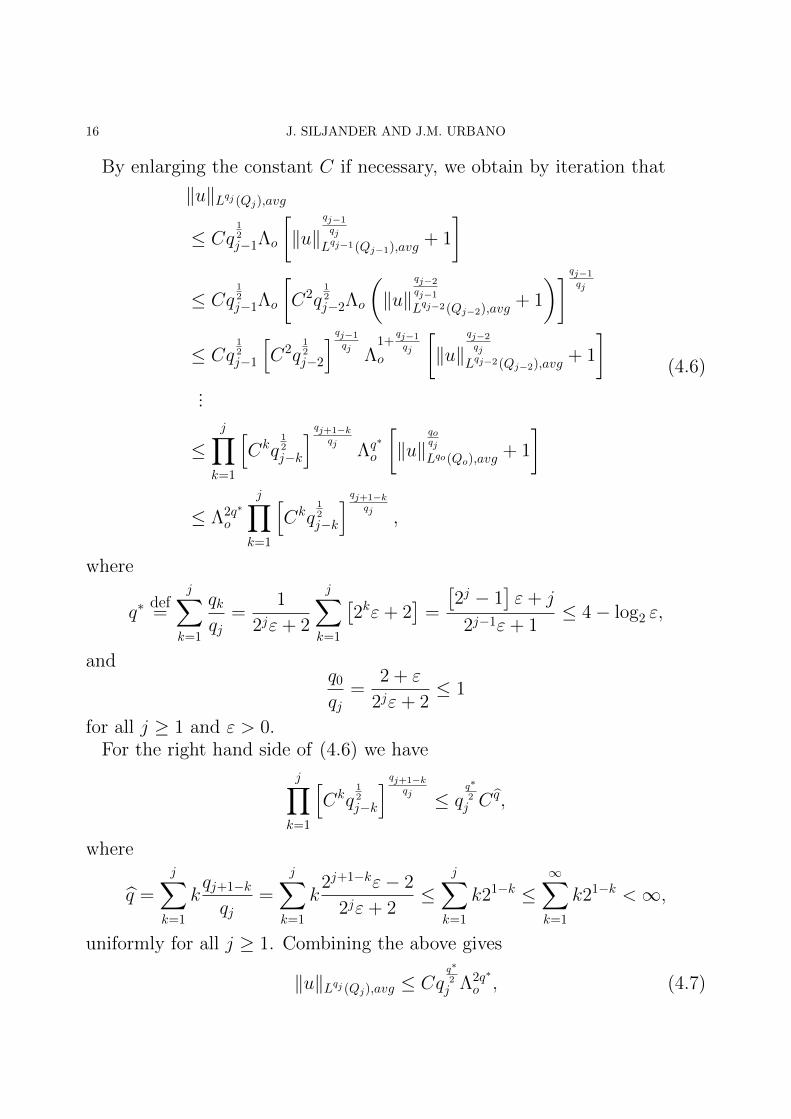
By enlarging the constant C if necessary, we obtain by iteration that

‖u‖Lqj (Qj),avg

≤ Cq12

j−1Λo

[‖u‖

qj−1qj

Lqj−1(Qj−1),avg+ 1

]≤ Cq

12

j−1Λo

[C2q

12

j−2Λo

(‖u‖

qj−2qj−1Lqj−2(Qj−2),avg

+ 1

)] qj−1qj

≤ Cq12

j−1

[C2q

12

j−2

] qj−1qj

Λ1+

qj−1qj

o

[‖u‖

qj−2qj

Lqj−2(Qj−2),avg+ 1

]...

≤j∏

k=1

[Ckq

12

j−k

] qj+1−kqj

Λq∗

o

[‖u‖

qoqj

Lqo(Qo),avg+ 1

]

≤ Λ2q∗

o

j∏k=1

[Ckq

12

j−k

] qj+1−kqj

,

(4.6)

where

q∗def=

j∑k=1

qkqj

=1

2jε+ 2

j∑k=1

[2kε+ 2

]=

[2j − 1

]ε+ j

2j−1ε+ 1≤ 4− log2 ε,

andq0

qj=

2 + ε

2jε+ 2≤ 1

for all j ≥ 1 and ε > 0.For the right hand side of (4.6) we have

j∏k=1

[Ckq

12

j−k

] qj+1−kqj ≤ q

q∗2

j Cq,

where

q =

j∑k=1

kqj+1−k

qj=

j∑k=1

k2j+1−kε− 2

2jε+ 2≤

j∑k=1

k21−k ≤∞∑k=1

k21−k <∞,

uniformly for all j ≥ 1. Combining the above gives

‖u‖Lqj (Qj),avg ≤ Cqq∗2

j Λ2q∗

o , (4.7)


for a uniform constant C independent of j.

Step 5. Let k ≥ 2 and choose j such that

k ≤ qj = 2jε+ 2 ≤ 2k.

Plugging this into (4.7) yields

−∫Qr

|u|k dµ ≤ Ckkkq∗2 Λ2q∗k

o

for all k ≥ 2. Using this to estimate the right hand side in (4.4) gives

esssupt∈I r2

−∫B r

2

|u(x, t)|k dx ≤ Ckkk2 Λk

o

[1 +−

∫Qr

|u|k dµ]

≤ [CΛcoo ]kkcok,

for k ≥ 2, and

codef= 2q∗ + 1.

By using the previous estimate, together with Holder’s inequality, we obtain,for an integer γ ≥ 1, that

−∫B r

2

eγ√|u(x,t)| dx ≤ −

∫B r

2

∞∑k=0

|u(x, t)|kγ

k!dx

≤∞∑k=0

1

k!−∫B r

2

|u(x, t)|kγ dx

≤ C

[−∫B r

2

|u(x, t)| dx+ 1

] 1γ

+

γ2−1∑k=2

[CΛcoo ]

kγk

cokγ

k!

+∞∑

k=γ2

[CΛcoo ]

kγk

cokγ

k!

uniformly for all t ∈ I r2. By Stirling’s formula, there exists a uniform constant

C1 such that, by choosing γ = C1coΛo, we obtain for the tail

∞∑k=γ2

[CΛcoo ]

kγk

cokγ

k!≤

∞∑k=γ2

[CC1

]kkk

k!≤ 1.


We finally get

esssupt∈I r2

−∫B r

2

eγ√|u(x,t)| dx ≤ C(ε,Λo),

where

Λo = Λo(Qo) = esssupt∈Io−∫Bo

|u| dx

+C

(r2−∫Qo

|ω|2 dµ+ 1

) 12(−∫Qo

|u|2+ε dµ+ 1

) 12+ε

,

for a uniform constant C. This finishes the proof.

Remark 4.1. The above proof of the main theorem only relies on the vortic-ity estimates (VE) for the weak solutions of the Euler equation and on theBiot-Savart law of Lemma 3.1. Therefore, the whole argument can also becompleted for weak solutions of the incompressible Navier-Stokes system

∂tu−∆u+ (u · ∇)u = −∇p.Indeed, the diffusive viscosity term ∆u will only add a positive contributionon the left hand side of (VE). This can also be used to absorb the additionalterm appearing in the vorticity formulation

∂tω −∆ω + (u · ∇)ω + (ω · ∇)u = 0

in higher dimensions.Consequently, it is an easy exercise to show that there exists a constant

C = C(αo) > 0 such that, for every α ≥ αo > 0, the vorticity formallysatisfies the energy estimate

esssup0≤t≤T

∫Ω

|ω|1+αζ2(x, t) dx+

∫ T

0

∫Ω

|∇|ω|1+α2 |2ζ2 dx dt

≤ C

∫ T

0

∫Ω

|ω|1+α

[|u||∇ζ|+ χd>2|u|2ζ2 +

(∂ζ

∂t

)+

]dx dt,

(4.8)

for every non-negative test function ζ ∈ C∞(ΩT ) vanishing on the parabolicboundary ∂pΩT . Observe that here one requires the existence of weak gra-dients for ω. A rigorous treatment removing this assumption requires anapproximation argument, for which we refer to [25].

The above energy estimate now includes a term of the form |u|2|ω|1+α, inaddition to |u||ω|1+α. Therefore, for the higher-dimensional Navier-Stokes


system the assumptions of Theorem 2.1 must be modified to ω ∈ Ldloc andu ∈ Lκ+ε

loc , for

κ =

2 if d = 2,2dd−2 if d ≥ 3.

(4.9)

The modifications, to extend Theorem 2.1 for the Navier-Stokes system, arestraightforward and we omit the details, even though we exploit this in thenext section, where we use our methodology to conclude the Serrin regularitytheorem [22].

5. On the interior regularity for Navier-StokesWe will now comment on how our reasoning can be used to give a modified

proof of the classical Serrin regularity theorem [22] for weak solutions of theincompressible Navier-Stokes system

∂tu−∆u+ u · ∇u = −∇p,∇ · u = 0,

(5.1)

in a space-time cylinder ΩT ⊂ Rd × R+. Moreover, we will also show howthe assumptions can be slightly relaxed in two dimensions, while acknowl-edging that the original goal of Serrin was to consider the case d ≥ 3;the well-posedness of the two-dimensional Navier-Stokes system had alreadybeen established by the seminal contributions of Leray, Hopf and Ladyzhen-skaya [18, 13, 17].

Theorem 5.1. Suppose

u ∈ L∞loc(0, T ;L2loc(Ω)) ∩ Lqloc(0, T ;Lsloc(Ω))

is a weak solution of the Navier-Stokes system (5.1) such that ω ∈ L2loc(ΩT )

and

q, s > 2, if d = 2,

2

q+d

s≤ 1 if d ≥ 3. (5.2)

Then u ∈ C∞ in the space variable with locally bounded derivatives.

Remark 5.1. The result is originally due to Serrin [22], where (5.2) is as-sumed also for d = 2. In addition to providing a slightly modified argumentfor the result, we observe that this requirement can be relaxed in two dimen-sions to just assuming q, s > 2.


Observe that – similarly to Serrin – we do not assume the existence ofSobolev gradients, which makes it possible to apply our method also for theEuler equations, as we have seen. If one assumes that the solution is a prioriin the energy space with full Sobolev gradients, then one may use the Sobolevembedding to obtain that a function satisfying our condition also satisfies theoriginal Serrin condition in two dimensions. The borderline case of equalityin (5.2) is originally due to Fabes, Jones and Riviere [11]. Later on, differentarguments have been provided, for instance, by Struwe [25].

We also exclude the case q =∞ and s = d, where important contributionshave been made in the three-dimensional case, for instance, by Escauriaza,Seregin and Sverak [10].

Proof : The Navier-Stokes and the Euler equations have different scalings andfor this reason we redefine the space-time cylinders by setting

σQ = σB × σI = B(0, σr)× (−σr2, 0),

for σ > 0. Let 0 < δ < 1 and choose a standard cut-off function ζ ∈C∞((1 + δ)Q) such that ζ = 0 on ∂p(1 + δ)Q with ζ = 1 in Q, and

|∇ζ| ≤ C

δras well as

∣∣∣∣∂ζ∂t∣∣∣∣ ≤ C

(δr)2.

We may now apply the energy estimate (4.8) for the vorticity formulation ofthe Navier-Stokes equations.

Let 0 < r < 1 be so small that

Q3r = B3r(0)×(− 3r2, 0

)⊂ B3r(0)× (−3r, 0)

def= U b Ω× (0, T ).

Assume first that u is in Lp, for p large enough. We will later use Theorem 2.1and the subsequent Remark 4.1 to prove this. We obtain from the parabolic


Sobolev embedding (2.3) and the energy estimate (4.8) that−∫I

(−∫B

(|ω|

1+α2

)s∗dx

) q∗s∗

dt

2q∗

≤ C

−∫(1+δ)I

(−∫

(1+δ)B

(|ω|

1+α2 ζ)s∗

dx

) q∗s∗

dt

2q∗

≤ C

(esssup(1+δ)I−

∫(1+δ)B

|ω|1+αζ2(x, t) dx+ r2−∫

(1+δ)Q

∣∣∇(|ω| 1+α2 ζ)∣∣2 dµ)≤ Cr2−

∫(1+δ)Q

|ω|1+α

[|u||∇ζ|+ χd>2|u|2ζ2 +

(∂ζ

∂t

)+

]dµ

≤C(1 + r2‖u‖Lp,avg

)δ2

−∫

(1+δ)Q

|ω|(1+α) pp−2 dµ,

(5.3)

for every p > 1 and for every (1 + δ)Q b ΩT , as well as for every 2 < s∗, q∗ <∞ with

d

s∗+

2

q∗≥ d

2. (5.4)

Now we may choose

q∗ = s∗ = 2

(1 +

2

d

)and p large enough to guarantee that

s∗

2>

p

p− 2.

This allows us to conclude, by a standard Moser iteration, that

esssupQr|ω| ≤ C

(−∫Q2r

|ω|2 dµ)1/2

,

where the constant C depends on the locally uniform bound of ‖u‖Lp. This isachieved by iterating (5.3) for increasing values of α, starting with α = 1. Thetheorem now follows as in Serrin [22] from the standard iterative argumentof using the convolution representation of ω in terms of u.


It remains to show the Lp-boundedness of u in Q2r. For d = 2, we imme-diately obtain, from Theorem 2.1 and Remark 4.1, that if

u ∈ L∞(I3r;L1(B3r)) ∩ L2+ε(U) for some ε > 0,

then u ∈ Lp(U), for all p > 1, which finishes the proof. For higher dimen-sions, we need to show that the assumptions of Theorem 2.1 hold. Thiscan be done in a manner similar to [25], but instead of proving that ω ∈L∞(2I;Ld+ε(2B)), it is enough to show that

ω ∈ Ld(2Q) ∩ L∞(2I;L2+ε(2B)) (5.5)

for some ε > 0. Indeed, by Lemma 2.1, we have that if ω ∈ L∞(I;L2+ε(B)),we directly obtain from the Biot-Savart law of Lemma 3.1 that

u ∈ Lκ+ρ(Q(2r)),

for κ as in (4.9), and ρ = ρ(ε) > 0. This is then enough to conclude theproof as described in the Remark 4.1.

We proceed similarly to [25]. By using the fact that u ∈ Lqloc(Lsloc) we may

use Holder’s inequality to control the term containing |ω|1+α|u|2, on the righthand side of (5.3), as

‖|ω|1+α|u|2ζ2‖L1 ≤ ‖ωζ2

1+α‖1+α

L(1+α)qo

2

(L

(1+α)so2

)‖u‖2Lq(Ls)(spt ζ), (5.6)

where

sodef=

2s

s− 2and qo

def=

2q

q − 2.

In order to improve the integrability of ω with the above estimate we needto guarantee that

s∗ ≥ so and q∗ ≥ qo. (5.7)

In this case we may absorb the term obtained in (5.6) to the left hand sideof (5.3) by choosing the support of the test function small enough. This ispossible as long as the pair (qo, so) satisfies the condition (5.4), i.e.,

d

2≤ d

so+

2

qo= 1 +

d

2− d

s− 2

q.

This yields the Serrin condition (5.2) for s and q. Finally, the result followsfrom iterating (5.3) for increasing values of α. For the details we refer to [25],where the only difference is that we may conclude the iteration already afterobtaining (5.5).


References[1] L. Ambrosio. Transport equation and Cauchy problem for BV vector fields. Invent. Math. 158

(2004), no. 2, 227–260.[2] C. Bardos and E. Titi. Euler equations for incompressible ideal fluids. Russian Math. Surveys

62 (2007), no. 3, 409–451.[3] F. Bouchut and G. Crippa. Lagrangian flows for vector fields with gradient given by a singular

integral. J. Hyperbolic Differ. Equ. 10 (2013), no. 2, 235–282.[4] T. Buckmaster, C. De Lellis, Ph. Isett and L. Szekelyhidi Jr. Anomalous dissipation for 1/5-

Holder Euler flows. Ann. of Math. 182 (2015) no. 1, 127–172.[5] P. Constantin. On the Euler equations of incompressible fluids. Bull. Amer. Math. Soc. (N.S.)

44 (2007), no. 4, 603–621.[6] P. Constantin, W. E and E. Titi. Onsager’s conjecture on the energy conservation for solutions

of Euler’s equation. Comm. Math. Phys. 165 (1994), no. 1, 207–209.[7] E. De Giorgi. Sulla differenziabilita e l’analiticita delle estremali degli integrali multipli rego-

lari. Mem. Accad. Sci. Torino. Cl. Sci. Fis. Mat. Nat. (3) 3 (1957), 25–43.[8] C. De Lellis and L. Szekelyhidi, Jr. The Euler equations as a differential inclusion. Ann. of

Math. (2) 170 (2009), no. 3, 1417–1436.[9] R. DiPerna and P.-L. Lions. Ordinary differential equations, transport theory and Sobolev

spaces. Invent. Math. 98 (1989), no. 3, 511–547.[10] L. Escauriaza, G. Seregin and V. Sverak. Backward uniqueness for parabolic equations. Arch.

Ration. Mech. Anal. 169 (2003), no. 2, 147–157.[11] E.B. Fabes, B.F. Jones Jr. and N.M. Riviere. The initial value problem for the Navier-Stokes

equations with data in Lp. Arch. Rational Mech. Anal. 45 (1972), 222–240.[12] U. Gianazza and V. Vespri. Parabolic De Giorgi classes of order p and the Harnack inequality.

Calc. Var. Partial Differential Equations 26 (2006), no. 3, 379–399.

[13] E. Hopf. Uber die Anfangswertaufgabe fur die hydrodynamischen Grundgleichungen. Math.Nachrichten 4 (1950-51), 213–231.

[14] Ph. Isett. Holder continuous Euler flows in three dimensions with compact support in time.arXiv:1211.4065v4 [math.AP], 2014.

[15] A. Kiselev and V. Sverak. Small scale creation for solutions of the incompressible two-dimensional Euler equation. Ann. of Math. (2) 180 (2014), no. 3, 1205–1220.

[16] A. Kiselev and A. Zlatos. Blow up for the 2D Euler equation on some bounded domains. J.Differential Equations 259 (2015) no. 7, 3490–3494.

[17] O.A. Ladyzhenskaya. Solution in the large to the boundary-value problem for the Navier-Stokes equations in two space variables. Soviet Physics Dokl. 123 (1958) no. 3, 1128–1131.

[18] J. Leray. Sur le mouvement d’un liquide visqueux emplissant l’espace. Acta Math. 63 (1934),pp. 193–248.

[19] A.J. Majda and A.L. Bertozzi. Vorticity and incompressible flow. Cambridge Texts in AppliedMathematics 27. Cambridge University Press, 2002.

[20] J. Moser. On Harnack’s theorem for elliptic differential equations. Comm. Pure Appl. Math.14 (1961), 577–591.

[21] V. Scheffer. An inviscid flow with compact support in space-time. J. Geom. Anal. 3 (1993),no. 4, 343–401.

[22] J. Serrin. On the interior regularity of weak solutions of the Navier-Stokes equations. Arch.Arch. Rational Mech. Anal. 9 (1962), 187–195.

[23] A. Shnirelman. On the nonuniqueness of weak solution of the Euler equation. Comm. PureAppl. Math. 50 (1997), no. 12, 1261–1286.


[24] E.M. Stein. Singular integrals and differentiability properties of functions. Princeton Mathe-matical Series 30. Princeton University Press, 1970.

[25] M. Struwe. On partial regularity results for the Navier-Stokes equations. Comm. Pure Appl.Math. 41 (1988), no. 4, 437–458.

[26] A. Vasseur. A new proof of partial regularity of solutions to Navier-Stokes equations. NoDEANonlinear Differential Equations Appl. 14 (2007), no. 5-6, 753–785.

Juhana SiljanderUniversity of Jyvaskyla, Department of Mathematics and Statistics, P.O. Box 35, FI-40014 University of Jyvaskyla, Finland.

E-mail address: [email protected]

Jose Miguel UrbanoCMUC, Department of Mathematics, University of Coimbra, 3001-501 Coimbra, Portugal.

E-mail address: [email protected]

on the interior regularity of weak … e-publica˘coes do departamento de matem atica universidade...

Documents