on the combined effect of periodic signals and coloured

On the Combined Effect of Periodic Signals and Coloured Noise

on Velocity Uncertainties

Anna Klos1, German Olivares2,3, Felix Norman Teferle2, Addisu Hunegnaw2 and Janusz Bogusz1 1) Military University of Technology, Faculty of Civil Engineering and Geodesy, Warsaw, Poland, e-mail: [email protected] 2) University of Luxembourg, Geophysics Laboratory, FSTC, Luxembourg, Luxembourg 3) CRC for Spatial Information, Melbourne, Australia

A B S T R A C T

The velocity estimates and their uncertainties derived from position time series of Global

Navigation Satellite System (GNSS) stations are affected by seasonal signals and their

harmonics, and the statistical properties, i.e. the stochastic noise, contained in the series. If the

deterministic model (linear trend and periodic terms) to describe the time series is not accurate

enough, then this will alter the stochastic model and the resulting effect on the velocity

uncertainties can be perceived as a consequence of a misfit of the deterministic model applied to

the time series. In other words, the effect of insufficiently modeled seasonal signals will

propagate into the stochastic model and falsify the results of the noise analysis besides the

velocity estimates and their uncertainties. In this study we provide the General Dilution of

Precision (GDP) of velocity uncertainties as being a ratio between uncertainties of velocities

determined when two different deterministic models are applied while accounting for stochastic

noise at the same time. In this newly defined GDP the first deterministic model includes a linear

trend, while the second one includes a linear trend and seasonal signals. These two are tested

with the assumption of power-law noise in the data. The more seasonal terms were added to the

series, the more biased the velocity uncertainties become, especially for short time scales. With

the increasing time span of observations, the assumption of seasonal signals becomes less

important and the power-law character of the residuals starts to play a crucial role in the

determined velocity uncertainties. With reference frame and sea level applications in mind we

argue that even smaller change in GDP than 5% could be considered as significant. This means,

that 7 and 9 years of continuous observations is the threshold for white and flicker noise, while

mailto:[email protected]

The General Dilution of Precision of Velocity Uncertainties

2

17 years are required for random-walk to make GDP to decrease below 5% and to omit periodic

oscillations in the GNSS-derived time series taking only the noise model into consideration.

Key words: Time-series analysis; Numerical modeling; Satellite geodesy; Reference systems.

1 I N T R O D U C T I O N

Today, Global Navigation Satellite System (GNSS) measurements, in particular those from the Global

Positioning System (GPS), are fundamental to many geodetic and geophysical investigations and are

frequently used during the construction of kinematic reference frames, such as the International Terrestrial

Reference Frame 2014 (ITRF2014) (Altamimi et al. 2016). From the processing or re-processing of the

observables of permanently installed GNSS stations, daily or weekly geocentric coordinate solutions are

obtained, from which position time series are formed. The primary product from the analysis of these time

series is often the linear rate of change, or velocity, and the associated uncertainty (Zhang et al. 1997).

The velocities are assumed to represent the linear movement of the Earth’s crust or land due to tectonic plate

motions (Larson et al. 1997, Altamimi et al. 2012) or the viscoelastic relaxation associated with glacial

isostatic adjustment (GIA) (Johansson et al. 2002, Bradley et al. 2009). Besides this, almost all sites within

the global network of GPS stations also show some non-linear, periodic motions, which have been associated

primarily with the seasonal changes on Earth. However, some stations may also exhibit motions of non-

linear and non-periodic character (Shih et al. 2008, Bogusz 2015). This may be due to the elastic response of

the Earth’s crust from the rapid ice mass loss at the polar ice sheets or mountain glaciers (Wahr et al. 2013),

being located in the deforming zones near plate boundaries (Wdowinski et al. 2004) or areas of oil and gas or

groundwater extraction (Munekane et al. 2004). In this study we will not deal with cases showing such non-

linear and non-periodic behavior.

Blewitt & Lavallée (2002) were one of the first to investigate the effect of periodic signals on GPS time

series and today it is widely acknowledged that such seasonal terms affect GPS and other geodetic time

series (e.g. Bos et al. 2010, Davis et al. 2012). The causes are almost completely recognized and can be

grouped into categories suggested by Dong et al. (2002): real geophysical effects of atmospheric (e.g.


3

Tregoning & van Dam 2005), hydrological (e.g. van Dam et al. 2001) or ocean loadings (e.g. van Dam et al.

2012) with thermal expansion (Romagnoli et al. 2003) and numerical artifacts of navigation satellite

systems. Penna & Stewart (2003) described aliased periodic signals in the coordinate time series due to

under-sampling of residual diurnal and semi-diurnal tidal signatures. Griffith & Ray (2013) extended this

analysis for the largest waves in the International Earth Rotation and Reference Frame Service (IERS)

Conventions 2010 diurnal and semi-diurnal tidal polar motion model assuming 24-h sampling. The second

technique-related error is associated with satellite orbits (draconitics). Agnew & Larson (2007) found that for

daily sampling rates in GPS-derived coordinates this period will alias to a frequency of 1.04333 cpy. Ray et

al. (2008) compared harmonics obtained using different techniques (GPS, VLBI and SLR) when they

discovered an anomalous peak in the GPS derived time series, which was not present in other series. They

explained it to be related to the interval required for the constellation to repeat its inertial orientation with

respect to the sun (GPS year). Amiri-Simkooei (2013) upon the analysis of the JPL (Jet Propulsion

Laboratory) data processed at the GPS Analysis Center obtained a period of 351.6±0.2 days. Finally,

multipath (King et al. 2012), insufficient modeling of antennas (Sidorov 2016), errors in network, the

adjustment that transfer from fiducial stations or the inclusion of the scale (Tregoning & van Dam 2005)

contribute to constellation-specific periodic signals in the time series.

From this it is clear that the deterministic model of a GNSS position time series needs to include the

parameters for both the linear and periodic motions at a given station (Bevis & Brown, 2014). Furthermore,

in a true geodetic approach the model must provide a means to obtain the most realistic uncertainties

associated with the parameter estimates in order to provide confidence limits at a given significance level for

these. In this respect, we model the time series, which have been pre-processed for outliers, offsets and gaps,

with Least Squares Estimation as:

ttAStACtvxtxn

i

Ti

iTi

i 1

0 sincos (1)

where x0, v, ACi, ASi, n are the intercept, velocity, cosine and sine terms of ith harmonic and the number of

harmonics of angular velocity of period T, respectively. The term ε(t) contains the residuals, all variations

not explicitly modeled and, therefore, disregarded by this station motion model. It is now commonly known


4

that the residuals do not follow a strict random (white noise with spectral index κ = 0) behavior but follow

that of a combination of white and coloured noise, with the latter often being modeled as a power-law

process (Agnew 1992). This temporally-correlated noise is due to mismodelling in GNSS satellites orbits,

Earth Orientation Parameters, large-scale atmospheric or hydrospheric effects (flicker noise with spectral

index κ = -1; Williams et al. 2004, Beavan 2005, Amiri-Simkooei et al. 2007, Bos et al. 2008, Teferle et al.

2008, Kenyeres & Bruyninx 2009, Santamaria-Gomez et al. 2011, Klos et al. 2015a), or the local

environment and monumentation (random walk process with spectral index κ = -2; Johnson & Agnew 1999,

Beavan 2005). Even when a perfect monument is considered with the environment being transparent to the

signal, the noise would be flicker and arise from low-frequency fluctuations of the satellite clocks (Dutta &

Horn 1981). Beyond the above, there are also some seasonal features that add more correlated noise to GNSS

data. As stated by Johnson & Agnew (1999), if time series were too short, it is more difficult to detect any

change due to correlation than it would be for long data. As is now widely acknowledged the stochastic

properties, i.e. the stochastic model of the residuals significantly influence the magnitude of the uncertainties

associated with the parameters (Zhang et al. 1997, Langbein & Johnson 1997, Mao et al. 1999, Williams

2003) and the whiter the noise, the faster the velocity uncertainty decays with increasing time series length.

Therefore, the noise character has the greatest impact on velocity uncertainty and errors of the deterministic

model estimated at the same time.

In this research we provide a General Dilution of Precision (GDP) of the velocity uncertainties being the

ratio of uncertainties of velocities arising from two different assumptions of the deterministic model. The

first of them assumes a linear velocity only, while the second is a combination of linear velocity and periodic

components. Each of the assumptions is presented with certain noise models starting from white, moving on

to flicker and end up with random walk, the most extreme case for GNSS position time series. The

determined errors of the velocities are being discussed along the two previous papers of Blewitt & Lavallée

(2002) and Bos et al. (2010) which provided the first discussion of this topic. We show using simulated data

that our approach gives additional advantages to GNSS time series analysis in comparison to the ones

mentioned before. Finally we apply the newly developed formulae to real GNSS time series of selected

stations in Europe.


5

2 D I L U T I O N O F P R E C I S I O N

Blewitt & Lavallée (2002) developed a model to calculate the bias level while one may not account for

periodic signals of annual frequency. The velocity bias expressed in mm/yr introduced by them was a zero-

crossing oscillatory function of data span, tending to zero for infinitely long time series. According to this

function they discovered the “zero-bias theorem” for unbiased velocity near integer-plus-half years and

introduced the ratio of uncertainties of velocities v1 and v2. They called it the Dilution of Precision (DP) and

estimated its value as (Blewitt & Lavallée 2002):

2

12

2 sincos1

sincos

61

f

ff

f

ff

fDP (2)

where is the time span, v1 and v2 denote the velocity determined without and with accounting for periodic

terms of frequency f, respectively. Figure 1 shows the DP value which increases towards infinity when the

time span is shorter than 1 year. A number of maxima of oscillations in DP can be noticed for integer years.

These come from periodic terms in (1). For certain epochs starting from 1.5 years with a step of 1 year DP =

1. It results from the fact that the velocity uncertainties for a model with linear velocity and model with

seasonal terms added are equal to each other. Besides, for a time span longer than 3.5 years the DP < 1.05,

which means that the difference between both variances is below 5%. However, Blewitt & Lavallée (2002)

considered only white noise, in consequence assumed that the character of residuals ε has no or little impact

on the estimated uncertainties.

However, it is expected that when power-law noise is added, the time when the difference between both

variances is below 5% will increase, as the power-law noise process adds temporal correlation to the time

series. That is why Bos et al. (2010) discussed the results of Blewitt & Lavallée (2002) by empirically

analyzing the effect of periodic signals using six stations, but assuming a combination of white and coloured


6

noise. They noticed, that the choice of character of the stochastic part may be much more important than that

of the seasonal part in the deterministic model. This is due to the fact that velocity uncertainty depends

mostly on the spectral index and amplitude of the power-law process. They concluded that the knowledge of

the noise characteristics of GNSS time series is crucial when velocities and their uncertainties are

determined. Furthermore, they observed a shift in the minimum of the DP from the integer-plus-half years

towards integer-plus-a-quarter years position. In this paper we confirm the results found by Bos et al. (2010),

but deliver the mathematic formulas for that.

Figure 1. Dilution of precision for models: with linear velocity and linear velocity plus periodic signals (recomputated

from Blewitt & Lavallée 2002).

Let us assume that the vector of residuals ε arising from deterministic model matrix x̂ fitted into (1) are

computed from:

xxε ˆ (3)

Then we can write down the observations in (1) as:

εAθx (4)


7

where A is the model or design matrix, θ is a vector with parameters of the model and ε is the vector of

residuals. When the parameters of the model are determined by means of Maximum Likelihood Estimation

(MLE), θ is given by:

xCAACAθ 111ˆ

TT

(5)

with Cεε being the covariance matrix for the vector of residuals ε. The covariance matrix of the parameters of

the model is:

TACAC

1

ˆˆ (6)

If the vector of residuals ε follows a power-law process such as:

i

N

j

jijivwh

1

0

(7)

which is a convolution of white noise of pli

w ,0 and another white noise of wni

v ,0 where pl

and wn are the standard deviations of noise, respectively. N is the number of data, while h is defined by the

recursive formula (Bos et al. 2008):

0 ,12

1

1

0

ii

hih

h

i

i

(8)

with being the spectral index, which when appropriately assigned may characterize the stochastic part of

the time series (Mandelbrot & Van Ness 1968). Then the covariance matrix of the residuals can be written

as:

iNwn

N

j

Nijjplilhh

2

0

2C

(9)

or as:


8

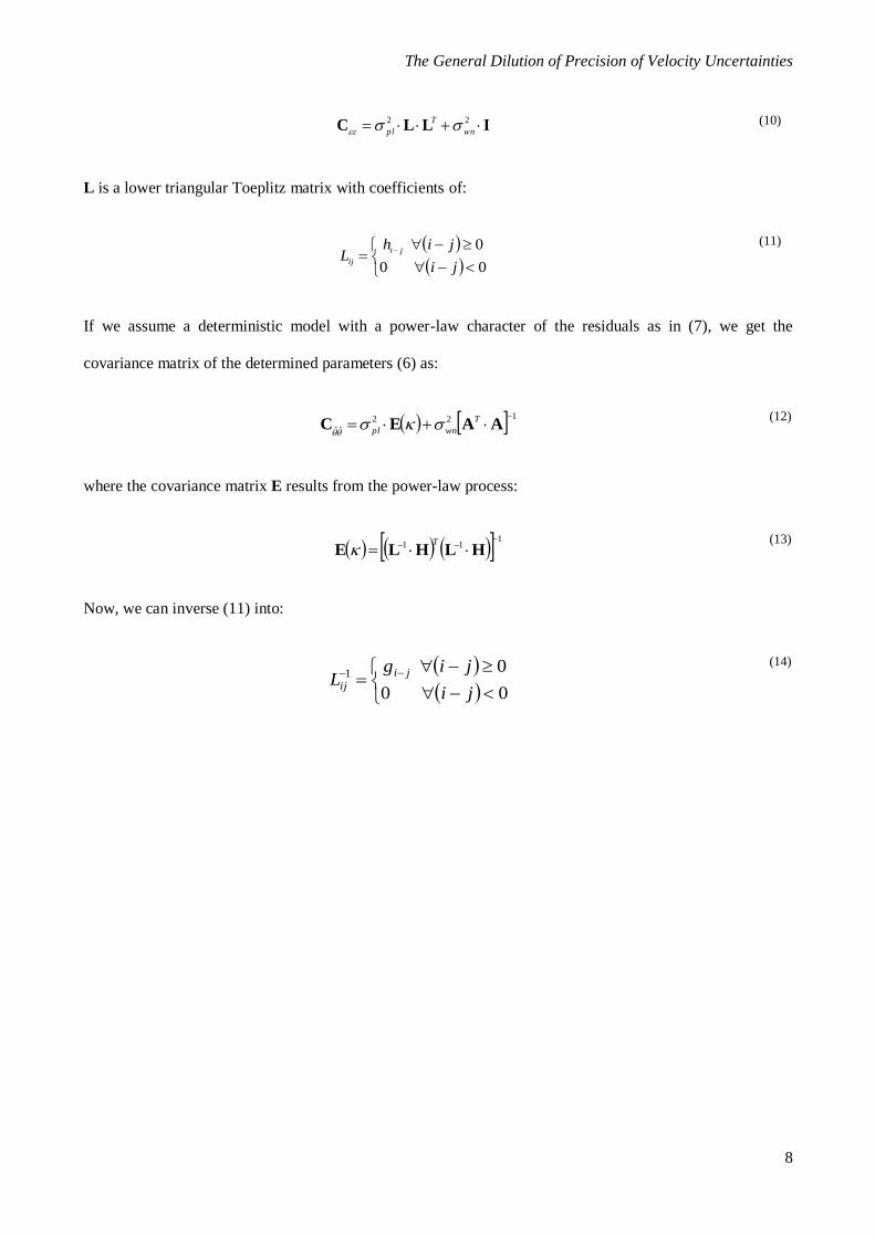
ILLC 22

wn

T

pl (10)

L is a lower triangular Toeplitz matrix with coefficients of:

0 0

0

ji

jihL

ji

ij

(11)

If we assume a deterministic model with a power-law character of the residuals as in (7), we get the

covariance matrix of the determined parameters (6) as:

122

ˆˆ

AAECT

wnpl

(12)

where the covariance matrix E results from the power-law process:

111

HLHLE

T

(13)

Now, we can inverse (11) into:

00

01

ji

ji gL

ji

ij

(14)


9

with:

0 ,12

1

1

0

ii

gig

g

i

i

(15)

These coefficients whiten any fractionally differenced Gaussian noise process as:

1

0

N

i

imim gw

(16)

with defined in (7).

3 M O D E L S

If we assume that the deterministic model of GNSS time series follows a linear trend with a vector of

parameters built as:

Tvx ,0

θ (17)

where v is the slope or velocity and x0 is the intercept and the model matrix A:

1

0

1

1

Nt

t

A (18)

then the variance of velocity that is estimated with the assumption of the general power-law process is

determined with:


10

N

iN

i

i

j

j

N

i

i

j

j

i

j

jiji

j

jij

pl

vv

g

gtg

tg

C

01

0

2

0

21

0 00

2

0

2

(19)

The proper modelling of the seasonal terms may directly influence on reliability of determined parameters,

such as the velocity. Blewitt & Lavallée (2002) showed, that seasonal term influences the uncertainty of

velocity. However, they did not consider the power-law character of residuals, but assumed them to follow a

white noise process. Bos et al. (2010) noticed that not only do the seasonal terms affect the linear velocity

when being improperly removed, but the noise properties are much more important for a reliable estimation

of the velocity error. These directly affect the uncertainty of velocity due to different shapes of covariance

matrix, as in (9-10).

Let us assume now a deterministic model with linear velocity and annual term:

111

000

2sin2cos1

2sin2cos1

NNNtftft

tftft

A

(20)

The vector of parameters is built here as:

TASACvx ,,,0

θ (21)

where AC and AS are the annual cosine and sine term, respectively.

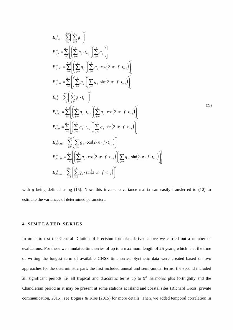
Now, we can compute the inverse of covariance matrix for the general power-law process 1E (13) as:

1

0

2

0

1

,

1

0 00

1

,

1

0

2

0

1

,

1

0 00

1

,

1

0 00

1

,

1

0

2

0

1

,

1

0 00

1

,

1

0 00

1

,

1

0 00

1

,

1

0

2

0

1

,

2sin

2sin2cos

2cos

2sin

2cos

2sin

2cos

0

0

0

00

N

i

i

j

jijASAS

N

i

i

j

jij

i

j

jijASAC

N

i

i

j

jijACAC

N

i

i

j

jij

i

j

jijASv

N

i

i

j

jij

i

j

jijACv

N

i

i

j

jijvv

N

i

i

j

jij

i

j

jASx

N

i

i

j

jij

i

j

jACx

N

i

i

j

j

i

j

jijvx

N

i

i

j

jxx

tfgE

tfgtfgE

tfgE

tfgtgE

tfgtgE

tgE

tfggE

tfggE

gtgE

gE

(22)

with g being defined using (15). Now, this inverse covariance matrix can easily transferred to (12) to

estimate the variances of determined parameters.

4 S I M U L A T E D S E R I E S

In order to test the General Dilution of Precision formulas derived above we carried out a number of

evaluations. For these we simulated time series of up to a maximum length of 25 years, which is at the time

of writing the longest term of available GNSS time series. Synthetic data were created based on two

approaches for the deterministic part: the first included annual and semi-annual terms, the second included

all significant periods i.e. all tropical and draconitic terms up to 9th harmonic plus fortnightly and the

Chandlerian period as it may be present at some stations at island and coastal sites (Richard Gross, private

communication, 2015), see Bogusz & Klos (2015) for more details. Then, we added temporal correlation in


12

form of white plus power-law noise, built an inverse covariance matrix as in (22) and transferred it to

estimate the variances of determined parameters as in (12). We assumed four different spectral indices equal

to 0, -1, -1.5 and -2 that indicate pure white, pure flicker, power-law noise between flicker and random-walk

process and pure random-walk noise, respectively, with 12 pl

and 12 wn

. White noise was added to

flicker, power-law and random-walk, when assumed.

Figure 2 shows the error of the velocity for white, flicker and random-walk noise. For time series shorter

than 70 days, the error of velocity is much higher for white and flicker noise assumptions than for random-

walk noise. This changes when data becomes to be longer than 70 days. The error of velocity is the smallest

for white noise assumption. Random-walk noise delivers the greatest errors of parameters. The longer the

data is, the greater is the difference between errors delivered for random-walk noise and flicker or white

noise assumptions. Having assumed white, flicker and random-walk noises, for 20 years of data, one will

obtain the error of velocity equal to 10-3, 10-2 and 10-1 mm/yr, respectively.

Figure 2. Error of velocity v (in mm/yr) for different lengths of time series in double logarithmic scale. The integer

spectral indices are examined. We assumed that 12 pl and 12 wn .

We estimated the relative differences in velocity variances for two deterministic models: with linear velocity

denoted as 2

1v and with linear velocity plus seasonal terms denoted as 22v as:


13

2

1

2

2

2

12

v

vvv

(23)

Adding seasonal terms results in oscillations in the estimated velocity error when the length of time series

changes. These of course are not so obvious any more, when a spectral index of power-law dependencies

increases. The same has been already noticed by Bos et al. (2010). The largest differences between two

models are being observed for the random-walk noise assumption. As the spectral index was shifted from 0

towards -3, the differences between velocity uncertainty will of course enlarge much more. Due to the above,

the largest differences between two models are being expected for badly monumented stations (Langbein &

Johnson 1997, Beavan 2005, Klos et al. 2015b).

A difference between the two uncertainties estimated with and without periodic terms can be better

understood by computing a ratio between them. We called it the General Dilution of Precision (GDP) in

accordance with Blewitt & Lavallée (2002) and as in (2), but taking into consideration a power-law noise in

the stochastic part, as was underlined in (12). We have adopted two approaches: widely used annual and

semi-annual terms to be subtracted and the approach consistent with Bogusz & Klos (2015): tropical and

draconitics up to their 9th harmonics plus Chandlerian and fortnightly. Figures 3 & 4 show a GDP for white,

flicker, random-walk and power-law noise of spectral indices equal to 0, -1, -2 and -1.5, respectively.


14

Figure 3. General Dilution of Precision (GDP) for white noise (blue), flicker noise (red), power-law noise of spectral

index equal to -1.5 (orange) and random-walk (green) plotted for deterministic model containing linear velocity plus

annual and semi-annual oscillations.

Figure 4. General Dilution of Precision (GDP) for white noise (blue), flicker noise (red), power-law noise of spectral

index equal to -1.5 (orange) and random-walk (black) plotted for deterministic model containing linear velocity plus

extended model of periodicities of all tropical and draconitic terms up to 9th harmonic plus fortnightly and the

Chandlerian period, according to Bogusz & Klos (2015).

Figure 5. Comparison between GDPs estimated for white noise (blue), flicker noise (red), power-law noise of spectral

index equal to -1.5 (orange) and random-walk (black) plotted for deterministic model containing 1) linear velocity plus


15

annual and semi-annual oscillations (dashed lines) and 2) linear velocity plus extended model of periodicities of all

tropical and draconitic terms up to 9th harmonic plus fortnightly and the Chandlerian period, according to Bogusz &

Klos (2015) (solid lines).

We computed the GDP values for harmonics of one year. They increased local maxima in the GDP plot. It

can be noticed that in comparison to Blewitt & Lavallée (2002) who considered the annual term, the semi-

annual signal also increases the local minimum of GDP with a white noise assumption. It means, that adding

the power-law noise to the annual curve or adding a semi-annual term to white noise causes an increase in

the velocity uncertainty even at those points where the estimated velocity should not be biased. The more

seasonal terms are added to the series, the more biased is the velocity uncertainty, especially for short time

scales. Having compared Figures 3 and 4 (Figure 5) it is clear, that the type of deterministic model affects the

velocity uncertainty and makes GDP to reach the value of 5% (we adopted this number following Blewitt &

Lavallée 2002) after 9 years, rather than 4, as was expected for annual plus semi-annual terms (a case of

white and flicker noise). The value of 5% means an increase in velocity uncertainty of 0.025 mm/yr, when a

typical error of velocity of 0.5 mm/yr is considered. However, with the increasing demand on velocities from

reference frame and sea level applications, we argue that even lower changes than 5% in GDP could be

considered as significant. All the above shows, that periodic terms affect the velocity uncertainty much more

at short time scales than they do for long-term data leaving the values of velocity unbiased. With the

increasing time span of observations, the assumption of seasonal signals becoming less important is

validated. Here, the power-law character of the residuals plays a crucial role in determining the velocity

uncertainty. In this way, 7, 9 and 17 years is enough, respectively, for white, flicker and random-walk to

make GDP to decrease below 5% and to omit periodic oscillations in the GNSS-derived time series taking

only noise model into consideration. So, providing a time series long enough, the assumed periodicities will

not affect the velocity uncertainty as much as the noise would. This is why we should focus on obtaining the

best estimate for the spectral index of each geodetic time series such as position, sea level or zenith total

delay.

5 R E A L G N S S T I M E S E R I E S


16

In order to confirm our theoretical approach above with real data we used position time series of continuous

GNSS stations produced at the Jet Propulsion Laboratory (JPL) using Precise Point Positioning (PPP)

(Zumberge et al. 1997) with integer ambiguities resolved (Bertiger et al. 2010). Further details on the data

processing strategy are published at: https://gipsy-oasis.jpl.nasa.gov. In this study we picked 115 stations

with time series of different lengths from 5 to 23 years and showing no specific or unusual behavior. This is

to ensure that our results are not compromised by stations, which, for example, did not follow the assumption

of a linear evolution in the coordinates. The station distribution is indicated in Figure 6. The daily time series

of the North, East and Up components were pre-processed for outliers, offsets and gaps if necessary and then

analyzed with the reformulated Maximum Likelihood Estimation (MLE) as implemented in the Hector

software (Bos et al. 2013). The stochastic model was assumed to be a combination of a white plus power-law

process along with two different deterministic models: (1) velocity and (2) velocity with all tropical and

draconitic terms up to 9th harmonic plus fortnightly and the Chandlerian period. Table 1 presents the results

of median seasonal amplitudes of annual (tropical), semi-annual, three- and four-monthly periods together

with their errors. The median amplitudes of the annual term are at the level of 1.65, 1.78 and 4.22±0.20 mm

for the North, East and Up component, respectively. Almost all median amplitudes of the 2nd, 3rd and 4th

harmonics of the annual term fall below 1 mm with a mean error equal to 0.10 and 0.25 mm for horizontal

and vertical changes.

The length of data of a minimum of 15 years is long enough for a noise process in GNSS time series to

become a dominant in GDP over seasonal signals. The ratio of velocity biases for the Up component is

rapidly varying in time due to the generally small values of the velocity itself. Hence, we decided not to

focus on it further.

Figure 6 presents GDP values for globally distributed set of stations of series of different lengths from 5 to

23 years. From these figures we can easily notice, that the GDPs for the North and East components remain

close to one for a majority of stations with minimum value of 0.94, maximum values of 1.04 and medians

close to 1.00. This is in good agreement with the theoretical formulae derived above. The greatest deviations

of values of GDP were obtained for stations affected by large seasonal signals, as e.g. BRAZ (Brazil) or

https://gipsy-oasis.jpl.nasa.gov/


17

KOUR (French Guiana). GDP for European stations generally tend to fall below 1% for all series examined

here.

6 C O N C L U S I O N S & D I S C U S S I O N

Not accounting for the seasonal signals results in an increase of the autocorrelation or temporally-correlated

noise within the time series. This, in turn, influences the stochastic model when the periodic signals are not

properly assumed. In this way, if we were certain about the presence of seasonal signals in the GNSS time

series and did not model them, the residuals would resemble more a flicker noise. This would lead to

increased uncertainties for all parameter estimates. Again, when the seasonal signals are properly modelled,

another issue that may cause an artificial increase in the velocity uncertainty is an improperly assumed noise

model itself. When flicker and random-walk are being compared to a power-law process there may be an

underestimation of the error bounds by a factor of two.

Some points can be easily noticed and raised for deeper discussion from the presented results. Along with the

increasing spectral index, the amplitudes of oscillations also increase. This arises from the fact that any

power-law process with κ<0 brings a correlation between amplitudes of seasonal terms and velocity. In this

way, the GDP value is much higher for any time series length considered. The strong peaks of oscillations as

seen in the GDP are indicated for short time scales, especially for the random-walk case. The applied

oscillations play a significant role, even much more important than the a priori assumed noise character. The

noise character starts to become important for time series longer than 9 years. The local minima and maxima

of GDP are also being enlarged together with a change of spectral index from 0 to -2. This shows, that the

GDP may differ from integer-plus-half years by Blewitt & Lavallée (2002), who considered only white

noise. This is clearly noticed for the case of random-walk and has already been empirically confirmed by

Bos et al. (2010). In this research, we provided mathematic formulas for the findings of Bos et al. (2010) and

confirm their correctness with synthetic and real data.

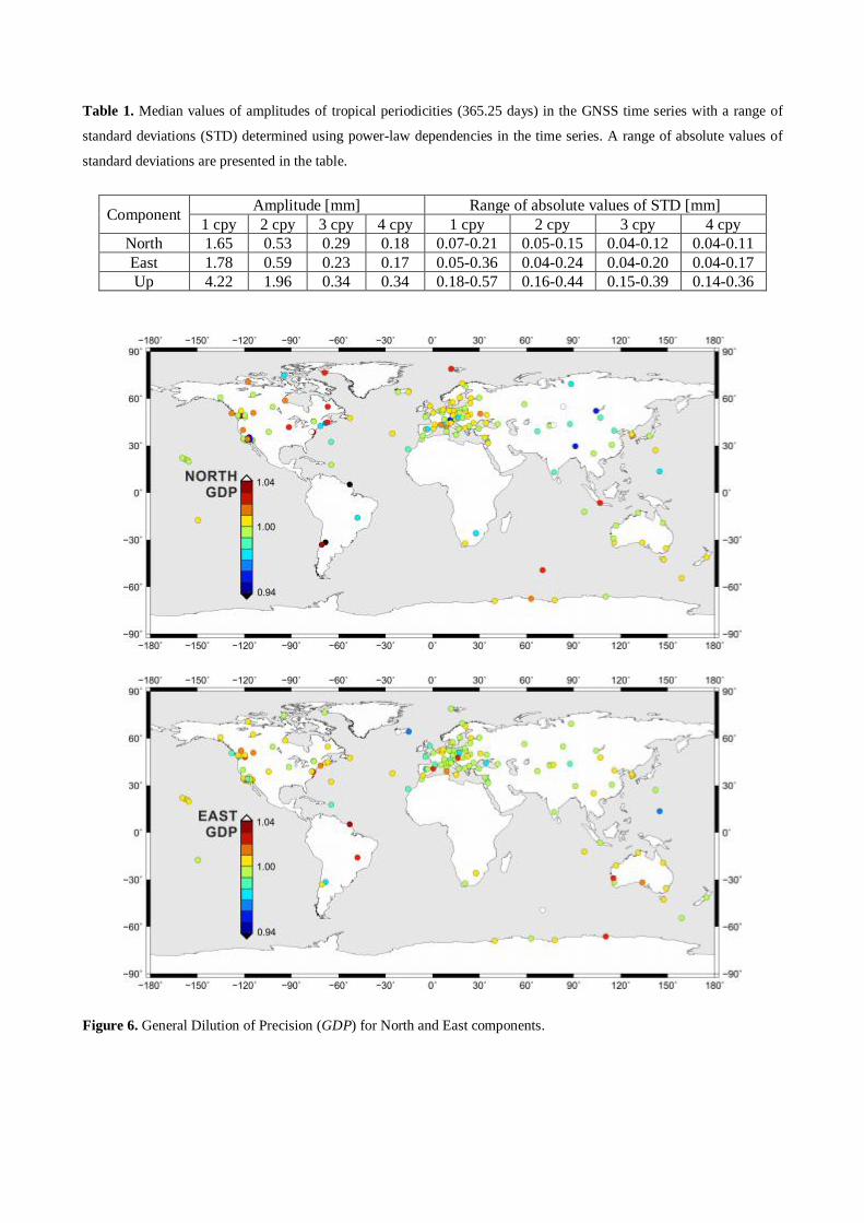
Table 1. Median values of amplitudes of tropical periodicities (365.25 days) in the GNSS time series with a range of

standard deviations (STD) determined using power-law dependencies in the time series. A range of absolute values of

standard deviations are presented in the table.

Component Amplitude [mm] Range of absolute values of STD [mm]

1 cpy 2 cpy 3 cpy 4 cpy 1 cpy 2 cpy 3 cpy 4 cpy

North 1.65 0.53 0.29 0.18 0.07-0.21 0.05-0.15 0.04-0.12 0.04-0.11

East 1.78 0.59 0.23 0.17 0.05-0.36 0.04-0.24 0.04-0.20 0.04-0.17

Up 4.22 1.96 0.34 0.34 0.18-0.57 0.16-0.44 0.15-0.39 0.14-0.36

Figure 6. General Dilution of Precision (GDP) for North and East components.


19

In this study we focused on white plus power-law noise, as generally the best estimate for the stochastic

model of GNSS time series. We showed that periodic signals are more important for short time scales,

whereas the stochastic noise plays a significant role when the length of the time series increases. Also, with

increasing spectral indices, the GDP decreases more slowly. We discussed a previously published approach,

which indicated that 3.5 years of data are enough for the GDP to fall below 5%. When more seasonal signals

and their harmonics were added to the deterministic model: periodicities of all tropical and draconitic terms

up to 9th harmonic plus fortnightly and the Chandlerian period, the GDP requires 9 years to fall below 5% for

white and flicker noise model. We have also discovered, that the noise character starts to become more

important than the periodic signals for time series longer than 9 years. And finally, Blewitt & Lavallée

(2002) used the value of 5% to calculate the minimum velocity bias. However, this value is disputable. With

the increasing demand on velocities, we argue that even smaller change in GDP could be considered as

significant. This means, that 7 and 9 years of continuous observations is the threshold for white and flicker

noise, while 17 years is enough for random-walk to make the GDP to decrease to below 5% and to omit

periodic signals in the GNSS-derived time series, taking only the noise model into consideration.

A C K N O W L E D G M E N T S

JPL repro2011b time series accessed from

ftp://sideshow.jpl.nasa.gov/pub/JPL_GPS_Timeseries/repro2011b/raw/ on 2015-08-13.

Maps in Fig. 6 were prepared with GMT software (Wessel et al., 2013).

Anna Klos and Janusz Bogusz are supported by the Faculty of Civil Engineering and Geodesy of the MUT

statutory research funds.

Addisu Hunegnaw is financed by the University of Luxembourg projects GSCG & SGSL.

R E F E R E N C E S

Agnew, D.C., 1992. The time-domain behaviour of power-law noises, Geophys. Res. Lett., 19(4), 333-336.

Agnew, D.C. & Larson, K.M., 2007. Finding the repeat times of the GPS constellation, GPS Solut. 11(1): 71–76,

doi:10.1007/s10291-006-0038-4.

Amiri-Simkooei, A.R., Tiberius, C.C.J.M. &Teunissen, P.J.G., 2007. Assessment of noise in GPS coordinate time

series: Methodology and results, J. Geophys. Res., 112(B07413), doi: 10.1029/2006JB004913, 2007.

Amiri-Simkooei, A.R., 2013. On the nature of GPS draconitic year periodic pattern in multivariate position time series.

J. Geophys. Res. Solid Earth, 118(5), 2500–2511, doi:10.1002/jgrb.50199.

Altamimi, Z., Rebischung, P., Métivier, L., & Collilieux, X., 2016. ITRF2014: A new release of the International

Terrestrial Reference Frame modeling nonlinear station motions, J. Geophys. Res. Solid Earth, 121, 6109–6131,

doi:10.1002/2016JB013098.

ftp://sideshow.jpl.nasa.gov/pub/JPL_GPS_Timeseries/repro2011b/raw/


20

Altamimi, Z., Métivier, L. & Collilieux, X., 2012. ITRF2008 plate motion model, J. Geophys. Res.: Solid Earth,

117(B7): B07402, doi:10.1029/2011JB008930.

Beavan, J., 2005. Noise properties of continuous GPS data from concrete pillar geodetic monuments in New Zealand

and comparison with data from U.S. deep drilled braced monuments, J. Geophys. Res., 110, B08410,

doi:10.1029/2005JB003642.

Bertiger, W., Desai, S., Haines, B., Harvey, N., Moore A., Owen S. & Weiss, J., 2010. Single receiver phase ambiguity

resolution with GPS data, J. Geod., 84(5): 327-337, doi:10.1007/s00190-010-0371-9.

Bevis, M. & Brown, A., 2014. Trajectory models and reference frames for crustal motion geodesy. J Geod, 88:283–311,

doi:10.1007/s00190-013-0685-5.

Blewitt, G. & Lavallée, D., 2002. Effect of annual signals on geodetic velocity, J. Geophys. Res., 107, 2145, doi:

10.1029/2001JB000570.

Bogusz J., 2015. Geodetic aspects of GPS permanent station non-linearity studies, Acta Geodyn. Geomater., 12, 4(180),

323-333, doi:10.13168/AGG.2015.0033.

Bogusz, J. & Klos, A., 2015. On the significance of periodic signals in noise analysis of GPS station coordinates time

series, GPS Solut., DOI: 10.1007/s10291-015-0478-9.

Bos, M.S., Fernandes, R.M.S., Williams, S.D.P. & Bastos, L., 2008. Fast Error Analysis of Continuous GPS

Observations, J. Geod., 82, pp. 157-166, doi: 10.1007/s00190-007-0165-x.

Bos, M., Bastos, L. & Fernandes, R.M.S., 2010. The influence of seasonal signals on the estimation of the tectonic

motion in short continuous GPS time-series. J. Geodyn., 49, 205-209, doi: 10.1016/j.jog.2009.10.005.

Bos, M. S., Fernandes, R. M. S., Williams, S. D. P., & Bastos, L., 2013. Fast Error Analysis of Continuous GNSS

Observations with Missing Data, J. Geod., 87(4), 351–360, doi:10.1007/s00190-012-0605-0.

Bradley, S. L., Milne G.A., Teferle F.N., Bingley R.M. & Orliac E.J., 2009. Glacial Isostatic Adjustment of the British

Isles: New constraints from GPS measurements of crustal motion, Geophys. J. Int., 178(1): 14-22,

doi:10.1111/j.1365-246X.2008.04033.x.

Davis, J.L., Wernicke, B.P. & Tamisiea, M.E., 2012. On seasonal signals in geodetic time series. J. Geophys. Res.,

117(B1), B01403, doi: 10.1029/2011JB008690.

Dong, D., Fang, P., Bock, Y., Cheng, M.K. & Miyazaki, S. 2002. Anatomy of apparent seasonal variations from GPS-

derived site position time series. J. Geophys. Res., 107, 2075, doi: 10.1029/2001JB000573.

Dutta, P. & Horn P.M., 1981. Low-frequency fluctuations in solids: 1/f noise, Rev. Mod. Phys. 53, 497.

Griffiths, J & Ray, J.R., 2013. Sub-daily alias and draconitic errors in the IGS orbits. GPS Solut 17(3): 413–422,

doi:10.1007/s10291-012-0289-1.

Johansson, J.M., Davis J.L., Scherneck H.G., Milne G.A., Vermeer M., Mitrovica J.X., Bennett R.A., Jonsson B.,

Elgered G., Elósegui P., Koivula H., Poutanen M., Rönnäng B.O. & Shapiro I.I., 2002. Continuous GPS

measurements of postglacial adjustment in Fennoscandia 1. Geodetic results, J. Geophys. Res.: Solid Earth,

107(B8): ETG 3-1-ETG 3-27.

Johnson, H.O. & Agnew, D.C., 1995. Monument motion and measurements of crustal velocities, Geophys. Res. Lett.,

22(21) pp. 2905-2908, doi: 10.1029/95GL02661.

Kenyeres, A. & Bruyninx, C., 2009. Noise and periodic terms in the EPN time series. Geodetic Reference Frames,

International Association of Geodesy Symposia 134, H. Drewes (ed.), doi:10.1007/978-3-642-00860-3_22,

Springer-Verlag, Berlin Heidelberg 2009.

King, M., Bevis M., Wilson T., Johns B. & Blume F., 2012. Monument-antenna effects on GPS coordinate time series

with application to vertical rates in Antarctica, J. Geod., 86(1): 53-63, doi: 10.1007/s00190-011-0491-x.

Klos, A., Bogusz, J., Figurski, M., Gruszczynska, M. & Gruszczynski, M., 2015a. Investigation of noises in the EPN

weekly time series. Acta Geodyn. Geomater., 2(178), doi:10.13168/AGG.2015.0010.

Klos, A., Bogusz, J., Figurski, M. & Kosek W., 2015b. Noise analysis of continuous GPS time series of selected EPN

stations to investigate variations in stability of monument types. Springer IAG Symposium Series volume 142,

proceedings of the VIII Hotine Marussi Symposium, doi:10.1007/1345_2015_62.

Langbein, J. & Johnson, H., 1997. Correlated errors in geodetic time series: Implications for time-dependent

deformation, J. Geophys. Res., 102(B1), pp. 591-603.

Langbein, J., 2012. Estimating rate uncertainty with maximum likelihood: differences between power-law and flicker-

random-walk models, J. Geod., 86: 775-783, doi:10.1007/s00190-012-0556-5.

Larson, K.M., Freymueller J.T. & Philipsen S., 1997. Global plate velocities from the Global Positioning system, J.

Geophys. Res., 102(B5): 9961-9981.

Mandelbrot, B. & Van Ness, J., 1968. Fractional Brownian motions, fractional noises, and applications, SIAM Rev 10,

pp. 422-439.

Mao, A., Harrison, Ch.G.A. & Dixon, T.H., 1999. Noise in GPS coordinate time series, J. Geophys. Res., 104(B2),

2797-2816.

Munekane, H., Tobita, M. & Takashima, K., 2004. Groundwater-induced vertical movements observed in Tsukuba,

Japan, Geophys. Res. Lett., 31, L12608, doi:12610.11029/12004GL020158.


21

Penna, N.T. & Stewart, M.P., 2003. Aliased tidal signatures in continuous GPS height time series. Geophys. Res. Lett.

30(23):2184. doi:10.1029/2003GL018828.

Ray, J., Altamimi, Z., Collilieux, X. & van Dam T., 2008. Anomalous harmonics in the spectra of GPS position

estimates. GPS Solut., 12(1): 55–64, doi:10.1007/s10291-007-0067-7.

Romagnoli, C., Zerbini, S., Lago, L., Richter, B., Simon, D., Domenichini, F., Elmi, C. & Ghirotti, M., 2003. Influence

of soil consolidation and thermal expansion effects on height and gravity variations. J. Geodyn., 35(4–5), 521–539,

doi: 10.1016/S0264-3707(03)00012-7.

Santamaria-Gomez, A., Bouin, M.N., Collilieux, X. & Woppelmann, G., 2011. Correlated errors in GPS position time

series: Implications for velocity estimates. J. Geophys. Res., 116, B01405, doi:10.1029/2010JB007701, 2011.

Shih, D.C.F., Wu, Y.M., Lin, G.F., Hu, J.C., Chen, Y.G. & Chang, C.H., 2008. Assessment of long-term variation in

displacement for a GPS site adjacent to a transition zone between collision and subduction, Stoch. Env. Res. Risk A.,

22(3), 401-410, doi:10.1007/s00477-007-0128-z.

Sidorov, D., 2016. Receiver Antenna and Empirical Multipath Correction Models for GNSS Solutions, PhD, University

of Luxembourg.

Teferle, F.N., Williams, S.D.P., Kierulf, K.P., Bingley, R.M. & Plag, H.P., 2008. A continuous GPS coordinate time

series analysis strategy for high-accuracy vertical land movements, Phys. Chem. Earth, 33, 205-216,

doi:10.1016/j.pce.2006.11.002.

Tregoning, P. & van Dam, T., 2005. Atmospheric pressure loading corrections applied to GPS data at the observation

level, Geophys. Res. Lett., 32, L22310, doi:10.1029/2005GL024104.

van Dam, T., Wahr, J., Milly, P.C.D., Shmakin A.B., Blewitt, G., Lavallée, D. & Larson, K.M., 2001. Crustal

displacements due to continental water loading, Geophys Res Lett, 28(4): 651–654.

van Dam, T., Collilieux, X., Wuite, J., Altamimi, Z. & Ray, J., 2012. Nontidal ocean loading: amplitudes and potential

effects in GPS height time series, J. Geod., 86:1043–1057, doi:10.1007/s00190-012-0564-5

Wahr, J., Khan, S.A., van Dam, T., Liu L., van Angelen, J.H., van den Broeke M.R. & Meertens C.M., 2013. The use of

GPS horizontals for loading studies, with applications to northern California and southeast Greenland, J. Geophys.

Res.: Solid Earth, 118(4): 1795-1806, doi:10.1002/jgrb.50104.

Wessel, P., Smith, W.H.F., Scharroo, R., Luis, J. & Wobbe, F., 2013. Generic Mapping Tools: Improved Version

Released, Eos, Trans. Amer. Geophys. Union., 94, 45(5), 409–410, doi:10.1002/2013EO450001.

Williams, S.D.P., 2003. Offsets in Global Positioning System time series. J. Geophys. Res., 108(B6), 2310,

doi:10.1029/2002JB002156.

Williams, S.D.P., Bock, Y., Fang, P., Jamason, P., Nikolaidis, R.M., Prawirodirdjo, L., Miller, M. & Johnson, D., 2004.

Error analysis of continuous GPS position time series, J. Geophys. Res., 109, B03412, doi: 10.1029/2003jb002741.

Wdowinski, S., Bock, Y., Baer, G., Prawirodirdjo, L., Bechor, N., Naaman, S., Knafo R., Forrai Y. & Melzer, Y., 2004.

GPS measurements of current crustal movements along the Dead Sea Fault, J. Geophys. Res., 109(B05403), 1-16,

doi:10.1029/2003JB002640. Zhang, J., Bock, Y., Johnson, H., Fang, P., Williams, S., Genrich, J., Wdowinski, S. & Behr, J., 1997. Southern

California permanent GPS geodetic array: error analysis of daily position estimates and site velocities, J. Geophys.

Res., 102(B8), 18,035-18,055.

Zumberge, J.F., Heflin, M.B., Jefferson, D.C., Watkins, M.M. & Webb, F.H., 1997. Precise point positioning for the

efficient and robust analysis of GPS data from large networks, J. Geophys. Res., 102(B3), 5005-5017.

on the combined effect of periodic signals and coloured

Documents