on smale’s 17th problem: a probabilistic positive solution
TRANSCRIPT

On Smale’s 17th Problem: A Probabilistic Positive
Solution.
Carlos Beltran 1,2,3, Luis Miguel Pardo 1,2
August 17, 2006
Abstract
Smale’s 17th Problem asks “Can a zero of n complex polynomialequations in n unknowns be found approximately, on the average [fora suitable probability measure on the space of inputs], in polynomialtime with a uniform algorithm?” We present a uniform probabilisticalgorithm for this problem and prove that its complexity is polynomial.We thus obtain a partial positive solution to Smale 17th Problem.
1 Introduction
In the first half of the nineties, Shub and Smale introduced a seminalconception of the foundations of numerical analysis. They focused on atheory of numerical polynomial equation solving in the series of papers[SS93a, SS93b, SS93c, SS94, SS96]. Other authors also treated this ap-proach in [Ren87, BCSS98, Ded01, Ded06, Kim89, Mal94, MR02, Yak95,CPHM01, CPM03] and references therein.
In these pages we complete part of the program initiated in the series[SS93a] to [SS94]. As in [SS94], the input space is the space of systems ofmultivariate homogeneous polynomials with dense encoding and fixed degreelist. Namely, for every positive integer l ∈ N, let Hl ⊆ C[X0, . . . ,Xn] be thevector space of all homogeneous polynomials of degree l. For a list of degrees(d) := (d1, . . . , dn) ∈ N
n, let H(d) be the set of all systems f := [f1, . . . , fn]of homogeneous polynomials of respective degrees deg(fi) = di, 1 ≤ i ≤ n.In other words, H(d) :=
∏ni=1Hdi
. We denote by d := max{di : 1 ≤ i ≤ n}the maximum of the degrees. Note that if (d) = (1) := (1, . . . , 1), the vector
1Dept. de Matematicas, Estadıstica y Computacion. F. de Ciencias. U. Cantabria.
E–39071 SANTANDER, Spain. email: [email protected], [email protected] was partially supported by MTM2004-011673Granted by FPU program, Goverment of Spain.4AMS Classification: Primary 65H10, 65H20. Secondary 58C35.
1
space H(1) can be identified with the space of all n×(n+1) complex matrices.Namely,
H(1) = Mn×(n+1)(C) = Cn×(n+1).
We denote by N + 1 the complex dimension of the vector space H(d).Note that N +1 is the input length for dense encoding of multivariate poly-nomials. For every system f ∈ H(d), we also denote by V (f) the projectivealgebraic variety of its common zeros. Namely,
V (f) := {x ∈ IPn(C) : fi(x) = 0, 1 ≤ i ≤ n},
where IPn(C) is the n-dimensional complex projective space. Note that withthis notation V (f) is always a non-empty projective algebraic variety.
The following is a preliminary version of the main outcome of this man-uscript. For a full statement see Theorem 6 of Section 1.2.
Theorem 1 There is a bounded error probabilistic numerical analysis proce-dure that solves most systems of multivariate homogeneous polynomial equa-tions with running time polynomial in
n,N, d.
The probability that a randomly chosen system f ∈ H(d) is solved by thisprocedure is greater than
1 − 1
N.
This theorem is a positive, although probabilistic, answer to Problem 17 in[Sma00]. Namely, we give a positive answer to the following question.
Problem 1 (Smale, 2000) “Can a zero of n complex polynomial equa-tions in n unknowns be found approximately, on the average , in polynomialtime with a uniform algorithm?”
We present a uniform probabilistic algorithm for this problem and prove thatits complexity is polynomial. We thus obtain a partial positive solution toSmale’s 17th Problem in [Sma00].
Let us now review some technical notions we’ll need to rigorously stateour underlying main algorithm.
1.1 Advances and Overcoming Prior Difficulties
This subsection is devoted to introduce the algorithm that satisfies all theclaims of Theorem 1. It is an algorithm based on homotopic deformation (cf.[GZ79, HSS01, Mor83, Mor86, MS87b, MS87a]) as established in the seriesof papers by M. Shub and S. Smale (mainly [SS93a, SS96, SS94]). In termsof algorithmic design, it belongs to the family of “non–universal polynomialequation solvers” as defined in [Par95, BP06a, CGH+03].
2
We describe our algorithm in four levels. At each level we also introducethe required notions and the main notations to be used in the sequel.
As usual, the first level is devoted to fix the input/output structure of theprocedure. At this level we recall the notion of projective Newton’s operator(as in [Shu93]) and the notion of approximate zero (as in [SS93a, BCSS98].
At a second level we fix the algorithmic scheme we use: Homotopicdeformation with prescribed resource data.
After this second level we are in conditions to fix the main drawback ofthis kind of algorithmic design: where to begin the homotopy in order toachieve tractable complexity bounds (i.e. a number of steps bounded by apolynomial in the input length). At this level we also discuss the notion ofε-efficient initial pair with prescribed resource function.
Third level is devoted to recall the main algorithmic scheme used toprove the main outcome in [SS94]. At this level we can also explain why themain outcome of [SS94] does not solve Problem 17 of [Sma00]. In [SS94],Shub & Smalke introduced an scheme which is either constructive nor provento be uniform.
We then arrive to a fourth level of detail and we describe our algorithmsatisfying the claims of Theorem 1.
Input/Output Structure. Our algorithm takes as input a system ofhomogeneous polynomial equations f ∈ H(d) and outputs local informationclose to some (mostly one) of the zeros ζ ∈ V (f). The local information wecompute is the information provided by an approximate zero z ∈ IPn(C) off associated with some zero ζ ∈ V (f) (in the sense of [SS93a, BCSS98]).
Projective Newton’s operator was introduced in [Shu93]. Let (f, z) ∈H(d) × IPn(C) be a pair. Let z⊥ := {w ∈ C
n+1 : 〈w, z〉 = 0} be the tangentspace of IPn(C) at z. If the restriction of the tangent mapping of f at z,Tzf := dzf |z⊥ , is nonsingular, we define the Newton iteration of f at z as:
Nf (z) := z − (Tzf)−1f(z) ∈ IPn(C).
According to [SS93a], an approximate zero z ∈ IPn(C) of a systemf ∈ H(d) with associated zero ζ ∈ V (f) ⊆ IPn(C) is a projective point
such that the sequence of iterates (Nkf (z))k∈N is well-defined and converges
to the actual zero ζ ∈ V (f) at a speed which is doubly exponential in thenumber of iterations. In this sense, an approximate zero is an ideal outputfor a polynomial system solving algorithm: Approximate zeroes occupy fewbits on average (cf. [CPM03]), yet they are close enough to true zeroes forNewton’s operator to converge quickly and efficiently yield any desired levelof accuracy.
The algorithms we consider will have the following input/output struc-ture:
3
Input: A system of homogeneous polynomial equations f ∈ H(d).
Output: An approximate zero z ∈ IPn(C) of f associated with some zeroζ ∈ V (f).
Such algorithms are built with the possibility of measure zero “bad” setof inputs (usually called ill-conditioned, singular, or degenerate) on whichthe algorithm fails. Via certain modifications (such as modifying the defini-tion of approximate zero, restricting the inputs to integer coefficients, or con-sidering the nearest problem with given singularity structure), it is possibleto solve polynomial systems in complete generality. We will not pursue thesemore technical extensions, but let us least point out to the reader that theseissues are highly non-trivial already for numerical linear algebra and the set-ting of one polynomial in one variable (see e.g. [Zen05, LE99, ME98]). Ex-tensions of α-theory and deflation methods for degenerate roots are studiedin [Lec01, Lec02, Yak00, Par95, GHMP95, GHMP97, GHH+97, GHM+98,LVZ, GLSY05b, GLSY05a, DS01, BP06b] .
Let Σ ⊆ H(d) be the set of systems f such that V (f) contains a singularzero. We call Σ the discriminant variety. These pages are mainly concernedwith procedures that solve systems without singular zeros (i.e., systems f ∈H(d) \ Σ).
Algorithmic Scheme. Our main algorithmic scheme is Homotopic De-formation in the projective space (as described in [SS96, SS94]): Givenf, g ∈ H(d) \ Σ, we consider the “segment” of systems “between” f and g,
Γ := {ft := (1 − t)g + tf, t ∈ [0, 1]}.
If Γ ∩ Σ = ∅, there are non-intersecting and smooth curves of equations-solutions associated with this segment:
Ci(Γ) := {(ft, ζt) : ζt ∈ V (ft), t ∈ [0, 1]}, 1 ≤ i ≤ D :=
n∏
i=1
di.
Then, Newton’s operator may be used to follow closely one of these curvesCi(Γ) in the product space H(d) × IPn(C). This procedure computes someapproximate zero z1 associated with some zero of f (i.e., t = 1) starting atsome approximate zero z0 associated with g (i.e., from t = 0). The followingdefinition formalizes this strategy.
Definition 2 A Homotopic Deformation scheme (HD for short) with initialdata (g, z0) ∈ H(d) × IPn(C) and resource function ϕ : H(d) × R
+ −→ R+ is
an algorithmic scheme based on the following strategy:
Input: f ∈ H(d), ε ∈ R+.
4
Perform ϕ(f, ε) “homotopy steps” following the segment (1 − t)g + tf , t ∈[0, 1], starting at (g, z0), where z0 is an approximate zero of g associated withsome zero ζ0 ∈ V (g).
Output:
either failure, oran approximate zero z1 ∈ IPn(C) of f .
An algorithm following the HD scheme is an algorithm that constructs apolygonal line P with ϕ(f, ε) vertices. The initial vertex of P is the point(g, z0) and its final vertex is the point (f, z1) for some z1 ∈ IPn(C). The out-put of the algorithm is the value z1 ∈ IPn(C). The polygonal is constructedby “homotopy steps” (path following methods) that go from one vertex tothe next. Hence, ϕ(f, ε) is the number of homotopy steps performed by thealgorithm. Different subroutines have been designed to perform each one ofthese “homotopy steps”. One of them is projective Newton’s operator asdescribed in [Shu93, SS93a, Mal94].
The positive real number ε is currently used both to control the numberof steps (through the function ϕ(f, ε)) and the probability of failure (i.e.,the probability that a given input f ∈ H(d) is not solved in ϕ(f, ε) stepswith initial pair (g, z0)).
Efficient Initial Pairs. We desire initial pairs with optimal tradeoff be-tween number of steps and probability of failure. We clarify this as follows.
Definition 3 Let p ∈ R[T1, T2, T3, T4] be some fixed polynomial. Let ε > 0be a positive real number. We say that an initial pair (g, z0) ∈ H(d)× IPn(C)is ε-efficient for HD if the HD scheme with initial pair (g, e0) and resourcefunction
ϕ(f, ε) := p(n,N, d, ε−1), ∀f ∈ H(d), ε > 0,
satisfies the following property:
“ For a randomly chosen system f ∈ H(d), the probability that HD outputsan approximate zero of f is at least 1 − ε”.
In order to simplify notations, from now on we consider the polynomial pfixed as follows:
p(n,N, d, ε−1) := 18 · 104n5N2d3ε−2,
for every n,N, d ∈ N \ {0}, and for every ε ∈ R, ε > 0.The main outcome in [SS94] is that for every positive real number ε > 0,
there is at least one ε-efficient initial pair (gε, ζε) ∈ H(d) × IPn(C). Thisstatement was a major breakthrough for the efficient numerical resolution
5
of polynomial systems, and its impact is only slowly beginning to be under-stood. These ε-efficient pairs are used as follows.
Input: f ∈ H(d), ε ∈ R+.
• Compute (gε, ζε) (the ε-efficient initial pair whose existence is guaran-teed by [SS94]).
• Perform p(n,N, d, ε−1) homotopy steps following the segment (1−t)g+tf , t ∈ [0, 1], starting at (gε, ζε).
Output:
either failure, oran approximate zero z ∈ IPn(C) of f .
Note that this procedure may output failure instead of giving an ap-proximate zero of f . However, the probability that the procedure does theformer is bounded above by ε, and we can at least control ε.
However, the procedure has three main drawbacks. First of all, theauthors of [SS94] prove the existence of some ε-efficient initial pair, butthey give no hint about how to compute such a pair (gε, ζε). Note thatif there is no method to compute (gε, ζε), then the previous scheme is notproperly an algorithm (you cannot “write” (gε, ζε) and thus you cannot startcomputing). Shub and Smale used the term “quasi-algorithm” to explain theresult they obtained, whereas Problem 17th in [Sma00] asks for a “uniformalgorithm”. In a broad sense, the last scheme is close to an “oracle machine”where the initial pair (gε, ζε) is given by some undefinable oracle. Moreover,the lack of hints on ε-efficient initial pairs leads both to Shub & Smale’sConjecture (as in [SS94]) and to Smale’s 17th Problem.
A second drawback is the dependence of (gε, ζε) on the value ε.Thirdly, the reader should observe that the initial pair (gε, ζε) must
be solved before we can perform any computation. Namely, ζε must be anapproximate zero of gε. In fact, Shub & Smale in [SS94] proved the existenceof such (gε, ζε) assuming that ζε is a true zero of gε (i.e., ζε ∈ V (gε)).However, using [SS93a, Main Thm.] you can relax this condition to assumethat ζε is an approximate zero associated with some zero of gε. This meansthat you need to make some precomputation by solving gε provided thatyou know it.
Thus, any algorithm based on this version of HD requires some “a priori”tasks not all of them simple:First, you have to detect some system of equations gε such that some of
6
its zeros ζε yields an ε-efficient initial pair (gε, ζε). Secondly, you need to“solve” the system gε in order to compute some approximate zero associatedwith the exact solution ζε.
As computing either an exact or an approximate zero of some unknowngε does not seem a good choice, we should proceed in the opposite manner:Start at some complex point ζε ∈ IPn(C), given a priori. Then, prove thatthere is a system gε vanishing at ζε such that (gε, ζε) is an ε-efficient initialpair. The existence of such a kind of system gε for any given ζε ∈ IPn(C)easily follows from the arguments in [SS94]. But, once again, no hint onhow to find gε from ζε seems to be known.
Questor Sets. In these pages we exhibit a solution to these drawbacks.We choose a probabilistic approach and, hence, we can give an efficientuniform (i.e. true) algorithm that solves most systems of multivariate poly-nomial equations. This is achieved using the following notion.
Definition 4 A set G ⊆ H(d) × IPn(C) is called a correct test set (alsoquestor set) for efficient initial pairs if for every ε > 0 the probability that arandomly chosen pair (g, ζ) ∈ G is ε-efficient is greater than
1 − ε.
Note the analogy between these families of efficient initial systems andthe “correct test sequences” (also “questor sets”) for polynomial zero tests(as in [HS82, KP96] or [CGH+03]). A similar idea to that used here (i.e.constructing a questor set for deciding where to start an iterative algorithm)has been recently developed in [HSS01]. We prove the following result.
Theorem 5 For every degree list (d) = (d1, . . . , dn) there is a questor setG(d) for efficient initial pairs that solves most of the systems in H(d) in timewhich depends polynomially on the input length N of the dense encoding ofmultivariate polynomials.
The existence of a questor set for initial pairs G(d) ⊆ H(d)×IPn(C) yieldsanother variation (of a probabilistic nature) on the algorithms based on HDschemes. First of all, note that the set G(d) does not depend on the positivereal number ε > 0 under consideration. Thus, we can define the followingHD scheme based on some fixed questor set G(d).
Input: f ∈ H(d), ε ∈ R+.
• Guess at random (g, ζ) ∈ G(d).
7
• Perform a polynomial (in ε−1, n,N, d) number of homotopy steps fol-lowing the segment (1 − t)g + tf , t ∈ [0, 1], starting at (g, ζ).
Output:
either failure, oran approximate zero z ∈ IPn(C) of f .
Observe that the questor set G(d) is independent of the value ε underconsideration. However, the existence of such a questor set does not implythe existence of a uniform algorithm. In fact, a simple existential statementas Theorem 5 will not be better than the main outcome in [SS94]: We needto extract suitable elements of G(d) explicitly. Hence, we exhibit an algorith-mically tractable subset G(d) which is proven to be a questor set for efficientinitial pairs. It leads to a “uniform algorithm”, although probabilistic. Thisrather technical set can be defined as follows.
1.2 An answer to Smale’s 17th Problem.
Let ∆ be the diagonal matrix used in [Kos93, SS93b], (see [BCSS98, pg.236] for further bibliographical references). With this matrix, Shub & Smaledefined a Hermitian product 〈·, ·〉∆ on H(d) which is invariant under certainnatural action of the unitary group Un+1 on H(d) (see also Section 2 fordetails). We denote by || · ||∆ the norm on H(d) defined by 〈·, ·〉∆. ThisHermitian product 〈·, ·〉∆ also defines a complex Riemannian structure onthe complex projective space IP(H(d)). This complex Riemannian structureon IP(H(d)) induces a volume form dν∆ on IP(H(d)) and hence a measure onthis manifold. The measure on IP(H(d)) also induces a probability on thiscomplex Riemannian manifold (see Section 2). Moreover, for every subsetA ⊆ IP(H(d)) the probability ν∆[A] induced by dν∆ agrees with the Gaussian
measure of the cone A over A in H(d) (i.e., A modulo scaling yields A). Inthe sequel, volumes and probabilities in H(d) and IP(H(d)) always refers tothese probabilities and measures defined by 〈·, ·〉∆.
Let us now fix a point e0 := (1 : 0 : · · · : 0) ∈ IPn(C). Let
Le0 := {f = [f1, . . . , fn] ∈ H(d) : fi = Xdi−10
n∑
j=1
aijXj , aij ∈ C}.
Let Ve0 ⊆ H(d) be the complex vector space of all homogeneous systems inH(d) that vanish at e0. Namely,
Ve0 := {f ∈ H(d) : e0 ∈ V (f)}.
Note that Le0 is a subspace of Ve0.
8
Next, let L⊥e0 be the orthogonal complement of Le0 in Ve0 with respect
to the Hermitian product 〈·, ·〉∆ (see Section 2 for details). Note that L⊥e0 is
the family of all homogeneous systems f ∈ H(d) that vanish at e0 and suchthat its derivative de0f also vanishes at e0.
Let Y be the following convex subset set of the affine space R × CN+1:
Y := [0, 1] ×B1(L⊥e0) ×B1(H(1)) ⊆ R × C
N+1,
where B1(L⊥e0) is the closed ball of radius one in L⊥
e0 with respect to thecanonical Hermitian metric and B1(H(1)) is the closed ball of radius onein the space of n × (n + 1) complex matrices with respect to the standardFrobenius norm. We assume Y is endowed with the product space proba-bility.
Let
τ :=
√n2 + n
N,
and let us fix any mapping φ : H(1) −→ Un+1 such that for every matrixM ∈ H(1) of maximal rank, φ associates a unitary matrix φ(M) ∈ Un+1
satisfying Mφ(M)e0 = 0. In other words, φ(M) transforms e0 into a vectorin the kernel of M . Our statements below are independent of the chosenmapping φ that satisfies this property.
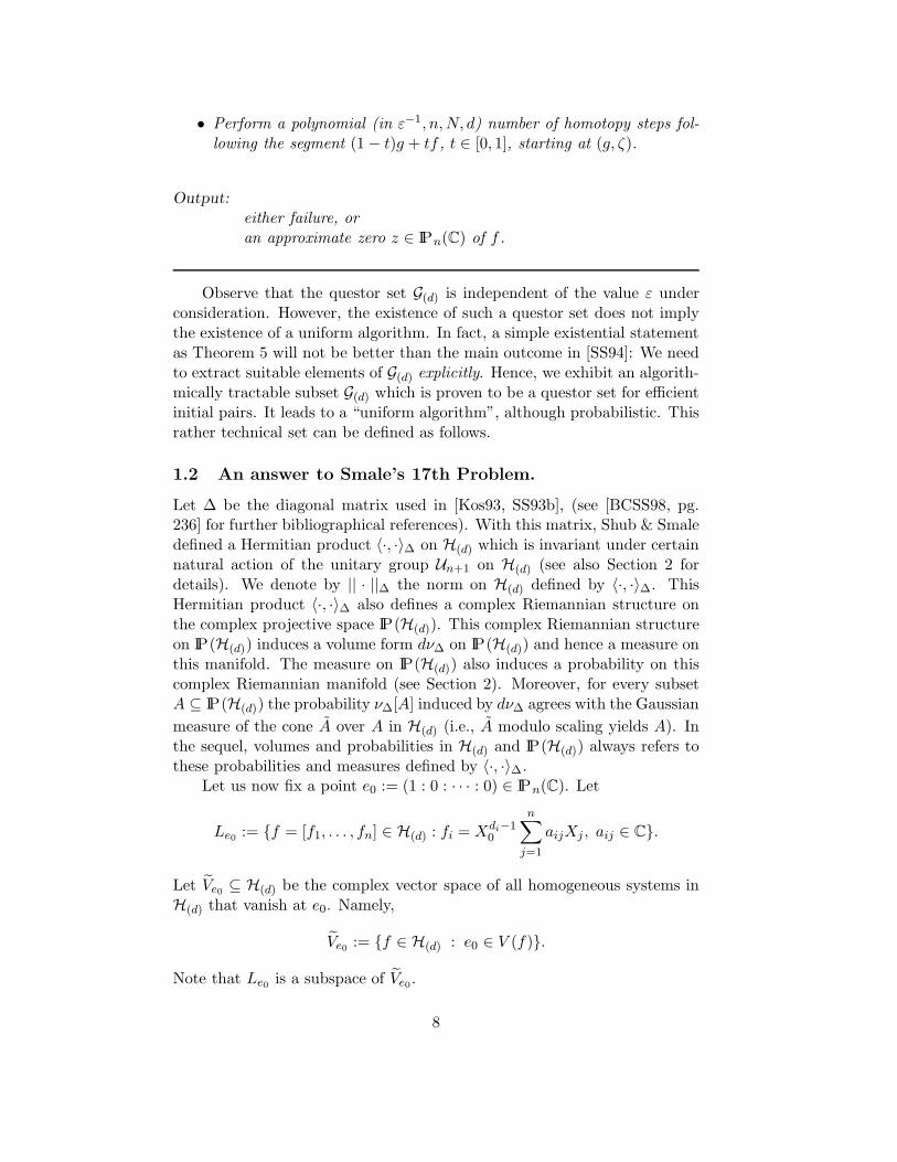
Let us define a mapping Θ : H(1) −→ Le0 as follows. For M ∈ H(1), let(aij : 1 ≤ i, j ≤ n) be the entries of Mφ(M). Namely,
Mφ(M) =
0 a11 · · · a1n...
.... . .
...0 an1 · · · ann
Then, we define Θ(M) = [f1, . . . , fn], where
fi = d1/2i Xdi−1
0
n∑
j=1
aijXj .
Define a mapping G(d) : Y −→ Ve0 as follows. For every (t, h,M) ∈ Y ,
let G(d)(t, h,M) ∈ Ve0 be the system of homogeneous polynomial equationsgiven by the identity:
G(d)(t, h,M) :=(1 − τ2t
1n2+n
)1/2 ∆−1h
||h||2+ τt
12n2+2n Θ
(M
||M ||F
)∈ Ve0,
where ‖ · ‖F is Frobenius norm. Finally, let G(d) be the set defined by theidentity:
G(d) := Im(G(d)) × {e0} ⊆ H(d) × IPn(C). (1)
Note that G(d) is included in the product Ve0 × IPn(C) since all the systemsf in Im(G(d) share a common zero e0 (i.e. f(e0) = 0). Hence initial pairs
9
in (g, z) ∈ G(d) always use the same exact zero z = e0. In particular, theyare all solved by construction.
We assume that the set G(d) is endowed with the pull-back probabil-ity distribution obtained from Y via G(d). Namely, in order to choose arandom point in G(d), we choose a random point y ∈ Y , and we compute(G(d)(y), e0) ∈ G(d). We present our main result.
Theorem 6 (Main Result) With the above notation, the set G(d) definedby identity (1) is a questor set for efficient initial pairs in H(d).
More precisely, for every positive real number ε > 0, the probability thata randomly chosen data (g, e0) ∈ G(d) is ε-efficient is greater than
1 − ε.
In particular, for these ε-efficient pairs (g, e0) ∈ G(d), the probability thata randomly chosen input f ∈ H(d) is solved by HD with initial data (g, e0)performing O(n5N2d3ε−2) homotopy steps is at least
1 − ε.
As usual, the existence of questor sets immediately yields a uniformprobabilistic algorithm. This is Theorem 1 above, which is an immediateconsequence of Theorem 6. The following corollary shows how this statementapplies.
Corollary 7 There is a bounded error probability algorithm that solves mosthomogeneous systems of cubic equations (namely inputs are in H(3)) in timeof order
O(n18ε−2),
with probability greater than 1 − ε.Taking ε = 1
n2 for instance, this probabilistic algorithm solves a cubichomogeneous system in running time at most O(n22) with probability greaterthan 1 − 1
n2 .
However, randomly choosing a pair (g, e0) ∈ G(d) is not exactly whata computer can perform. Under Church’s Thesis, computing is discrete.Thus, we need a discrete set of ε-efficient initial systems. This is achievedby the following argument (that follows similar arguments in [CPM03]).
Observe that Y ⊆ R × CN+1 may be seen to be a real semi-algebraic
set under the identification R × CN+1 ≡ R
2N+3. Let H ≥ 0 be a positiveinteger number. Let Z
2N+3 ⊆ R2N+3 be the lattice consisting of the integer
points in R2N+3. Let Y H be the set of points defined as follows:
Y H := Y ∩ 1
HZ
2N+3,
10
where 1HZ
2N+3 is the lattice given by the equality:
1
HZ
2N+3 := { zH
: z ∈ Z2N+3}.
For any positive real number H > 0, we denote by GH(d) ⊆ G(d) the finiteset of points given by the equality:
GH(d) := {(G(d)(y), e0) : y ∈ Y H}.
Then, the following statement also holds.
Theorem 8 There exists a universal constant C > 0 such that for everytwo positive real numbers ε > 0,H > 0 satisfying
log2H ≥ Cn2N3 log2 d+ 2 log2 ε−1,
the following properties hold.
• The probability (uniform distribution) that a randomly chosen data(g, e0) ∈ GH(d) is ε-efficient is greater than
1 − 2ε.
• In particular, for these ε-efficient initial pairs (g, e0) ∈ GH(d), the prob-ability that a randomly chosen input f ∈ H(d) is solved by HD withinitial data (g, e0) performing O(n5N2d3ε−2) steps is at least
1 − ε.
The lattice estimates in Theorem 8 immediately imply that our probabilisticpolynomial algorithm can be implemented on any standard digital computer.
Theorem 6 and its consequences thus represent a small step forward inthe theory introduced by Shub and Smale. It simply shows the existence ofa uniform, although probabilistic, algorithm that computes approximationsof some of the zeros of solution varieties for most homogeneous systemsof polynomial equations in time which depends polynomially on the inputlength. 5
This paper is structured as follows. In Section 2 we detail the nota-tion we will use, and we continue a series of results appearing in [Shu93,SS93a, SS93b, SS93c, SS94, SS96] that we use to prove our main theorems.We include a brief introduction to the projective Newton operator and theHomotopy Method in Section 3, although we encourage the reader to seethis in its original context in [Shu93, SS93a, SS94] or [BCSS98]. Section 5is devoted to proving Theorem 6 (and hence Theorem 1). Finally, Section 6contains the proof of Theorem 8.
5In the terminology of [Par95, CGH+03, BP06a] this simply means that there is a nonuniversal polynomial equation solver running in probabilistic polynomial time.
11

2 Basic Notation
2.1 Metrics
For every Hermitian vector space (F, 〈·, ·〉) of complex dimension m and forevery nonsingular matrix A ∈ GL(m,C), we denote by 〈·, ·〉A : F ×F −→ C
the Hermitian product given by the following identity:
〈x, y〉A := 〈Ax,Ay〉,
for all x, y ∈ F . Let us denote by || · || and || · ||A the norms on F respectivelydefined by the Hermitian products 〈·, ·〉 and 〈·, ·〉A.
For every positive real number t ∈ R+, we shall use the notationsSt(F ), Bt(F ), StA(F ), Bt
A(F ) to denote respectively the spheres and closedballs in F of radius t centered at the origin with respect to the correspondingHermitian products. For every subspace L ⊆ F , we shall denote by L⊥ theorthogonal complement of L in F with respect to some specified Hermitianmetric.
As in the Introduction, for every positive integer number l ∈ N, letHl ⊆ C[X0, . . . ,Xn] be the vector space of all homogenous polynomialsof degree l with complex coefficients. The monomial basis of Hl can beidentified with the set of multi-indices
Nn+1l := {µ = (µ0, µ1, . . . , µn) ∈ N
n+1 : |µ| := µ0 + · · · + µn = l}.
As in standard elimination theory we can choose a monomial order ≤l inNn+1l (see [CLO97, BW93, GPW03] and references therein for an introduc-
tion to monomial orders, Grobner bases and Computational CommutativeAlgebra). Any monomial order in N
n+1l allows us to see the elements of Hl
as vectors given by their coordinates (with respect to this monomial order).This is called in standard literature “dense encoding of polynomials”. LetNl be the complex dimension of Hl. For every µ ∈ N
n+1l , we define the
multinomial coefficient (l
µ
):=
l!
µ0! · · · µn!.
We define the matrix ∆l ∈ MNl(C) associated with Hl as the diagonal
matrix whose µ-th entry (with respect to the monomial order ≤l) at the
diagonal is( lµ
)−1/2. Namely, ∆l is the diagonal matrix given by the following
identity:
∆l := ⊕µ∈Nn+1l
((l
µ
)−1/2).
Let 〈·, ·〉l : Hl ×Hl −→ C be the canonical Hermitian product on Hl.
12
Let (d) := (d1, . . . , dn) ∈ Nn be a list of positive degrees. We also have
the canonical Hermitian product on H(d) given by the following identity:
〈f, g〉 :=
n∑
i=1
〈fi, gi〉di∈ C,
where f := [f1, . . . , fn], g := [g1, . . . , gn] ∈ H(d). We finally denote by 〈·, ·〉∆the Hermitian product over H(d) defined by the respective matrices ∆di
andgiven by the following identity:
〈f, g〉∆ :=
n∑
i=1
〈∆difi,∆di
gi〉di=
n∑
i=1
〈fi, gi〉∆di,
where f := [f1, . . . , fn], g := [g1, . . . , gn] ∈ H(d). We denote by ∆ the follow-ing matrix,
∆ :=n⊕i=1
∆di∈ MN+1(C).
In order to simplify the notation, we will denote respectively by S and S∆ thespheres S1(H(d)) and S1
∆(H(d)). The volume element in S will be denotedby dν.
2.2 Incidence Varieties.
We follow the notation used in the introduction. For every system f ∈ H(d),we also denote by f the mapping between complex affine spaces f : C
n+1 −→Cn.
Let e0 := (1 : 0 : . . . : 0) ∈ IPn(C) be a point that we may fix asa “north pole”. Let f ∈ H(d) be a system of homogeneous polynomialequations, and let ζ ∈ V (f) be any solution. We denote by Tζf the matrix(in some orthonormal basis) of the restriction of the tangent mapping dζf tothe tangent subspace TζIPn(C) = ζ⊥ ⊆ C
n+1 of all elements of Cn+1 which
are orthogonal to the complex line ζ ∈ IPn(C). In the case that ζ = e0 wemay identify Te0f and its matrix in the natural basis {e1, . . . , en}. Namely,
Te0f ≡
∂f1∂x1
. . . ∂f1∂xn
......
∂fn
∂x1. . . ∂fn
∂xn
∈ Mn(C).
For every ζ ∈ IPn(C), we shall denote by Vζ ⊆ H(d) the vector subspacegiven as the set of systems of homogeneous equations satisfied by ζ. Thatis,
Vζ := {f ∈ H(d) : f(ζ) = 0 ∈ Cn}.
Note that Vζ is a complex vector subspace of H(d) of complex codimensionn.
13

We define the incidence variety V ⊆ S∆ × IPn(C) given by the followingidentity:
V := {(f, ζ) ∈ S∆ × IPn(C) : ζ ∈ V (f)}.We also consider the two following canonical projections:
p1 : V −→ S∆, p1(f, ζ) := f,∀(f, ζ) ∈ V,
andp2 : V −→ IPn(C), p2(f, ζ) := ζ,∀(f, ζ) ∈ V.
We may obviously identify p−11 (f) ≡ V (f) and p−1
2 (ζ) ≡ Vζ ∩ S∆ = S1∆(Vζ).
From now on, we shall denote Vζ := p−12 (ζ).
The following statement summarizes the basic properties of V , and itsproof may be found in [BCSS98].
Proposition 9 The incidence variety V is a connected submanifold of theproduct manifold S∆ × IPn(C) of real codimension 2n. Moreover, the fibersVζ are submanifolds of V of real codimension 2n in V .
We shall denote by Σ′ ⊆ V the critical locus of p1, i.e. Σ′ := {(f, ζ) ∈V : Tζf 6∈ GL(n,C)} (cf. [BCSS98] for details). We also denote byΣ := p1(Σ
′) the critical values of p1 (also called the discriminant variety).As observed in [SS94], the following proposition follows from the implicitfunction theorem.
Proposition 10 (Shub & Smale) Let g ∈ S∆ be a point, and let L∆ ⊆S∆ be a (real) great circle in S∆ such that g ∈ L∆. Assume that L∆ ∩ Σ =∅. Then, p1 : p−1
1 (L∆) −→ L∆ is a D-fold covering map, and p−11 (L∆) \
p−11 ({−g}) consists of D open arcs in V . Let ζ ∈ V (g) be a solution of g.
We denote by ARCg,ζ the (unique) open arc of p−11 (L∆) \ p−1
1 ({−g}) thatcontains the point (g, ζ).
Note that the vector space Le0 defined at the Introduction is preciselythe set of ℓ ∈ Ve0 that satisfy Te0ℓ ≡ ℓ |e⊥0 (as linear operators). Then, L⊥
e0
is the subspace of those f ∈ Ve0 such that Te0f ≡ 0. Namely, it is the familyof all homogeneous systems of polynomial equations of order at least 2 ate0.
Let us denote by ∆(d)−1/2 ∈ Mn(C) the diagonal complex matrix givenby
∆(d)−1/2 :=
d−1/21 · · · 0...
. . ....
0 · · · d−1/2n
.
We finally define the mapping
ψe0 : Le0 −→ Mn(C)
14
ψe0(ℓ) := ∆(d)−1/2Te0ℓ,
As in [BCSS98, page 235], the following simple fact holds.
Proposition 11 The mapping ψe0 defines an isometry between Le0 withthe Hermitian product induced by the Hermitian product 〈·, ·〉∆ on H(d) andMn(C) with its canonical (Frobenius) Hermitian product.
Obviously, ψe0 also defines an isometry between the spheres St∆(Le0)and St(Mn(C)), identifying their respective Riemannian structures.
2.3 Some unitary actions.
Let Un+1 ⊆ Mn+1(C) be the group of unitary matrices. Every U ∈ Un+1
defines an isometry on the complex projective space: U : IPn(C) −→ IPn(C).The group Un+1 also defines an action on H(d) for every U ∈ Un+1 as follows,
f −→ f ◦ U−1.
The following statement was proved in [BCSS98].
Proposition 12 With the notation above, the Hermitian product 〈·, ·〉∆ isinvariant under the action of Un+1 over H(d). Namely, for all f, g ∈ H(d)
and for all U ∈ Un+1, the following equality holds:
〈f, g〉∆ = 〈f ◦ U−1, g ◦ U−1〉∆.
The manifold V is also invariant under the action of Un+1 on the productS∆ × IPn(C). Moreover, every U ∈ Un+1 defines isometries between thefibers of p2. In fact, given ζ, ζ ′ ∈ IPn(C) two projective points, and givenU ∈ Un+1, such that Uζ = ζ ′, then the mapping
U−1 : Vζ −→ Vζ′
f 7−→ f ◦ U−1
is an isometry. Obviously, the restriction
U−1 : Vζ = S1∆(Vζ) −→ Vζ′ = S1
∆(Vζ′)
is also an isometry between spheres. Moreover, the following mapping isalso an isometry for any U ∈ Un+1:
U : V −→ V
(f, y) 7→ (f ◦ U−1, Uy).
Observe that the following diagrams commute:
VU−→ V
p1 ↓ ↓ p1
S∆U−1
−→ S∆
VU−→ V
p2 ↓ ↓ p2
IPn(C)U−→ IPn(C)
15
Let f ∈ Ve0 be any system. We consider the following number:
DET (f, e0) := det(Te0f(Te0f)∗),
where the symbol ∗ denotes Hermitian transpose.The following statement is consequence of the results in [BCSS98].
Proposition 13 With the notation above, let (f, ζ) ∈ V be a regular pointof p1. Then, the following equality holds:
NJ(f,ζ)p1
NJ(f,ζ)p2=NJ(f◦U,e0)p1
NJ(f◦U,e0)p2= DET (f ◦ U, e0),
where U ∈ Un+1 is any matrix such that Ue0 = ζ and NJ(f,ζ)p1 andNJ(f,ζ)p2 are respectively the normal jacobians at (f, ζ) ∈ V of p1 and p2
(as defined for example in [BCSS98, 13.2]).
Proof.– In [BCSS98] this result is proven when considering the projectivespace IP(H(d)) instead of S∆. Now, we can check that this change does notaffect the calculus. The first equality is proved the same way as in [BCSS98].As for the second one, observe that for any element (f, e0) ∈ V , the tangentspaces TfS∆ and Tf IP(H(d)) differ only in the vector
√−1f ∈ TfS∆. Observe
that the vector (√−1f, 0) ∈ T(f,e0)V satisfies:
•√−1f = d(f,e0)p1(
√−1f, 0) is orthonormal to g = d(f,e0)p1(g, x) for
every (g, x) ∈ T(f,e0)V such that 〈(g, x), (√−1f, 0)〉T(f,e0)V = 0.
• (√−1f, 0) ∈ Ker(d(f,e0)p2).
Thus, the volume of the images under d(f,e0)p1 or d(f,e0)p2 of a unit cubecontained in the orthogonal complement of the respective kernel does notvary, and both normal jacobians NJ(f,ζ)p1 and NJ(f,ζ)p2 remain the samewhen considering S∆ or IP(H(d)).
2.4 Normalized Condition Numbers.
For every (f, ζ) ∈ V we shall denote by µnorm(f, ζ) the normalized conditionnumber introduced in [SS93a] (cf. also [SS93b] or [BCSS98]). Namely,
µnorm(f, ζ) := ‖(Tζf)−1∆(d)1/2‖2,
where the representatives ζ and f are chosen such a way that ‖ζ‖2 = ‖f‖∆ =1.
Condition numbers in Linear Algebra were introduced by A. Turing in[Tur48]. They were also studied by J. von Neumann and collaborators (cf.
16
[NG47]) and by J.H. Wilkinson (cf. also [Wil65]). Variations of these con-dition numbers may be found in the literature of Numerical Linear Algebra(cf. [Dem88], [GVL96], [Hig02], [TB97] and references therein).
The Condition Number κD of Linear Algebra is defined as follows: Forany square matrix A ∈ Mk(C), κD(A) := ‖A‖F ‖A−1‖2 . The followingstatement immediately follows from the definition of µnorm.
Proposition 14 With the notation above, the following equality holds forevery (f, ζ) ∈ V :
µnorm(f, ζ) =κD(∆(d)−1/2Tζf)
||∆(d)−1/2Tζf ||F,
where the representatives ζ and f are chosen such a way that ‖ζ‖2 = ‖f‖∆ =1.
Moreover, the normalized condition number µnorm is invariant underthe action of the unitary group Un+1. Namely, given (f, ζ) ∈ V and givenU ∈ Un+1, the following equality holds:
µnorm(f, ζ) = µnorm(f ◦ U−1, Uζ).
For every positive real number ε > 0, we also introduce the “tube”Σ′ε ⊆ V given by the following identity:
Σ′ε := {(f, ζ) ∈ V : µnorm(f, ζ) > ε−1}.
Note that Σ′ε is invariant under the action of Un+1. We recall the no-
tations of Section 2.2. Let g ∈ S∆ be a point. For every great circle L∆
containing g, L∆ ∩ Σ = ∅, and for every positive number ε > 0, we denoteby τ gε (L∆) the number of arcs of p−1
1 (L∆) \ p−11 ({−g}) that intersect the set
Σ′ε. In other words,
τ gε (L∆) := ♯{ζ ∈ V (g) : ARCg,ζ ∩ Σ′ε 6= ∅}.
This definition makes sense because of Proposition 10. Then, for everypositive real number ε > 0, and for every great circle L∆ ⊆ S∆ such thatL∆ ∩ Σ = ∅, we define
τε(L∆) := supg∈L
τ gε (L∆).
2.5 A volume estimate for great circles.
Let S × S and S∆ × S∆ be these Riemannian manifolds, with the productRiemannian structure. For respective measurable subsets A1 ⊆ S× S, A2 ⊆S∆ × S∆, we denote their respective volumes as ν[A1], ν∆[A2].
17
Let ∆−1 ∈ MN+1(C) be the inverse of the nonsingular matrix ∆. Ob-serve that both
∆−1 : S −→ S∆.
and∆−1 × ∆−1 : S × S −→ S∆ × S∆.
are isometries. Let L be the Riemannian manifold of great circles (realspherical lines) in S, endowed with the natural orthogonal-invariant Rie-mannian structure. We denote by dL the volume form associated with thisRiemannian structure. For every measurable subset A ⊆ L, let νL[A] be thevolume of A with respect to dL. We may assume that this volume form hasbeen normalized such a way that νL[L] = 1. We recall some basic propertiesof the Riemannian structures we have introduced. Let O2N+2 be the groupof orthogonal square matrices of size 2N + 2, which acts isometrically overCN+1 ≡ R
2N+2. Namely, for every measurable set A ⊆ S, the followingholds:
ν[A] = ν[OA], ∀O ∈ O2N+2.
The following mapping is an isometry for every orthogonal matrix O ∈O2N+2:
O : L −→ LL 7→ OL := {Of ∈ S : f ∈ L}.
For every element L ∈ L, we may consider the great circle L∆ ⊆ S∆ definedas L∆ := ∆−1L = {∆−1f : f ∈ L}. In Subsection 2.4, for every positivenumber ε > 0 and every great circle L∆ ⊆ S∆ not intersecting Σ, we havedefined the quantity τε(L∆). Thus, for every element L ∈ L such thatL∆ ∩ Σ = ∅ we can consider the number τ(ε, L) defined as follows.
τ(ε, L) := τε(L∆),
For every element f ∈ S∆ \Σ, we may consider the positive integer number♯(ε, f) ∈ N defined as follows:
♯(ε, f) := ♯{ζ ∈ V (f) : µnorm(f, ζ) > ε−1}.
We also denote by L∆ the set of all the (real) great circles in S∆. We recalla result of M. Shub and S. Smale, which can be found in [SS93b].
Theorem 15 (Shub-Smale) For every positive number ε > 0, the follow-ing inequality holds:
1
ν∆[S∆]
∫
f∈S∆
♯(ε, f) dS∆ ≤ n3(n+ 1)N2Dε4,
where D :=∏ni=1 di is the Bezout number.
18

The following result is also due to Shub and Smale, as it can be obtained asan immediate consequence of the corollary of Theorem 1 in [SS96].
Lemma 16 (Shub-Smale) For every positive real number ε > 0 and forevery L ∈ L, the following inequality holds:
τ(ε, L) ≤(cε2
d3/2
)−1 ∫
f∈L∆
♯(2ε, f) dL∆,
where c ≥ 0.09 is a universal constant.
Proof.– From the definition, τ(ε, L) = τε(L∆) = supg∈L∆τgε (L∆). Now,
from [SS94, Proof of Cor. 3.5] the quantity τgε (L∆) is bounded for every
g ∈ L by (cε2
d3/2
)−1 ∫
f∈L∆
♯(2ε, f) dL∆,
and the lemma follows.
The following result is implicitly stated in [SS94]. We include a shortproof for completeness.
Proposition 17 Let ε > 0 be a positive real number. The following in-equality holds.
∫
L∈Lτ(ε, L) dL ≤ 32π
cd3/2n3(n+ 1)N2Dε2,
where c > 0 is the universal constant of Lemma 16.
Proof.– From Lemma 16,
∫
L∈Lτ(ε, L) dL ≤
(cε2
d3/2
)−1 ∫
L∈L
∫
f∈L∆
♯(2ε, f) dL∆ dL =
=
(cε2
d3/2
)−1 ∫
L∈L
∫
f∈L♯(2ε,∆−1f) dL dL.
The following Santalo-type equality follows from Shub & Smale’s argumentsin [SS96, Prop. 4b] (cf. [How93, San76] for other similar Integral Geometryformulae):
∫
L∈L
∫
f∈L♯(2ε,∆−1f) dL dL = 2π
∫f∈S
♯(2ε,∆−1f) dS
ν[S].
As ∆−1 is an isometry from S to S∆,
1
ν[S]
∫
f∈S
♯(2ε,∆−1f) dS =1
ν[S∆]
∫
f∈S∆
♯(2ε, f) dS∆,
19
and Theorem 15 yields:
1
ν[S∆]
∫
f∈S∆
♯(2ε, f) dS∆ ≤ 16n3(n+ 1)N2Dε4.
Thus, ∫
L∈Lτ(ε, L) dL ≤
(cε2
d3/2
)−1
32πn3(n+ 1)N2Dε4,
and the proposition follows.
3 The Homotopy Method.
There is a wide bibliography on Newton-like methods for solving systemsof polynomial equations. Some good references are [BCSS98, Ded06, DS00,Mal94]. In [Shu93], the projective Newton operator is introduced, and theseries of papers [SS93a, SS93b, SS93c, SS94, SS96] propose a linear homotopymethod. We recall now the key ingredients of this method. Most of themare summarized in [BCSS98].
Let dT : IPn(C) × IPn(C) −→ R be the function given by the followingequality,
dT (z1, z2) := tan(dR(z1, z2)).
Namely, dT is the tangent of the Riemannian distance. Observe that dT isnot exactly a distance function, but dT (z1, z2) is very similar to dR(z1, z2)for small values of dR(z1, z2). Let ζ ∈ IPn(C) be a zero of f ∈ S∆.
Definition 18 We say that z ∈ IPn(C) is an approximate zero of f withassociated zero ζ if the sequence
z0 := z, zi+1 := Nf (zi) ∀i ≥ 0
is defined, and
dT (ζ, zi) ≤(
1
2
)2i−1
dT (ζ, z),∀i ≥ 0.
The following result guarantees the convergence of the Newton sequenceunder some assumptions:
Theorem 19 (Shub & Smale) Let f ∈ S∆, and let ζ ∈ IPn(C) be a zeroof f . Let γ0(f, ζ) be the number defined as follows.
γ0(f, ζ) := ‖ζ‖maxk≥1
∥∥∥∥(Tζf)−1Dkf(ζ)
k!
∥∥∥∥
1k−1
,
20
where Dkf(ζ) is the k-th derivative of f , considered as a k-linear map. Letz ∈ IPn(C) be such that
dT (z, ζ)γ0(f, ζ) ≤3 −
√7
2.
Then, z is an approximate zero of f with associated zero ζ.
3.1 The linear homotopy.
Observe that Theorem 19 does not solve the problem of finding a zero of agiven system f ∈ S∆. In fact, in general it may be hard to find an initialpoint z ∈ IPn(C) satisfying the conditions of Theorem 19. The linear homo-topy proposed by Shub and Smale solves this problem considering anothersystem g ∈ S∆, which has a known zero ζ0. Then, we consider the segment
Γ := {ft := (1 − t)g + tf, t ∈ [0, 1]} ⊆ H(d).
If Γ ∩ Σ = ∅, the implicit function theorem defines a path of solutions
C(Γ) := {(ft, ζt) : ζt ∈ V (ft), t ∈ [0, 1]}
Observe that ζ1 is a zero of f1 = f . Let k ≥ 1 be a positive integer,representing the number of homotopy steps to be done. Let ti = i
k , 0 ≤ i ≤k, and consider the following sequence of systems:
fti =
(1 − i
k
)g +
i
kf, 0 ≤ i ≤ k.
Observe that ft0 = g, ftk = f . Then, we may consider the sequence of pointsdefined as follows:
x0 := ζ0, xi+1 := Nfti+1(xi), 0 ≤ i ≤ k − 1.
The following is the main result of [SS93a] (see also [BCSS98, pg. 271] or[Bel06, Prop. 4.2.6]). It bounds the number of steps k that are necessary toguarantee convergence.
Theorem 20 (Shub & Smale) With the notations and assumptions above,let µ ∈ R be the number defined as follows:
µ := max0≤t≤1
µnorm(ft, ζt).
Let k ∈ N be such that k ≥ 18d3/2µ2. Then, for every 0 ≤ i ≤ k, xi is anapproximate zero of fti, with associated zero ζi/k. In particular, xk is anapproximate zero of f with associated zero ζ1.
21

In [SS94], a more intelligent method to construct the homotopy pathbetween two points is proposed. Practical implementations should followthis scheme, instead of the “fixed step size” scheme we propose here. How-ever, the theoretical results we prove are valid for both schemes. Observethat, as shown in the Introduction, the key ingredient for this method is theinitial pair (g, ζ0), satisfying the condition that µ is small for a wide set ofinput polynomials f .
4 A Series of Reductions.
In this section we will perform a series of geometric reductions from Shub &Smale’s statements above. The final expression will be used in the comingsections to prove the main theorems in the Introduction. Every subsectioncontains one of these reductions.
4.1 From great circles to pairs of systems of equations.
Let D ⊆ S × S be the antipodal diagonal in this product space. Namely,
D := {(f, g) ∈ S × S : f = ±g}.
We define the mapping
L : S × S \ D −→ L,
such that for every (f, g) ∈ S×S\D, the line L(f, g) ∈ L is the unique greatcircle in S that contains f and g. We also consider the set
D∆ := {(f, g) ∈ S∆ × S∆ : f = ±g},
and the mappingL∆ : S∆ × S∆ \ D∆ −→ L∆,
such that for every (f, g) ∈ S∆ × S∆ \ D∆, the line L∆(f, g) is the uniquegreat circle in S∆ that contains f and g.
Lemma 21 Let F : M −→ N be a map between complex or real Rie-mannian manifolds M,N . Let x, y ∈ M be two points in M . Assume thatthere exist isometries h : M −→ M and h1 : N −→ N such that h(x) = y,and the following formula holds:
h1 ◦ F = F ◦ h.
Then, NJxF = NJyF .
22
Proof.– As h and h1 are isometries,
(NJF (x)h1)(NJxF ) = NJx(h1 ◦ F ) = NJx(F ◦ h) =
= (NJh(x)F )(NJxh) = (NJyF )(NJxh).
Now, NJF (x)h1 = NJxh = 1 and the lemma follows.
We prove the following lemma:
Lemma 22 Let Φ : L −→ R be an integrable mapping. Then, the followingformula holds:
∫(f,g)∈S×S
Φ(L(f, g)) d(S × S)
ν[S]2=
∫
L∈LΦ(L) dL.
Proof.– The Coarea formula (see [Fed69, Mor88] or more recently [BCSS98])applied to the differentiable mapping L : S × S \ D −→ L, yields:
∫
(f,g)∈S×S
Φ(L(f, g)) d(S × S) =
∫
L∈LΦ(L)
∫
(f,g)∈L−1(L)
1
NJ(f,g)LdL−1(L) dL. (2)
We check that the inner integral is a constant. In fact, let L1, L2 ∈ L betwo great circles, and let O ∈ O2N+2 be an orthogonal matrix such thatOL1 = L2. Consider the following isometry:
O ×O : S × S \ D −→ S × S \ D
(f, g) 7→ (Of,Og).
Then, (O × O)|L−1(L1) is an isometry between L−1(L1) and L
−1(L2). TheCoarea Formula applied to this map yields:
∫
(f1,g1)∈L−1(L1)
1
NJ(f1,g1)LdL−1(L1) =
=
∫
(f2,g2)∈L−1(L2)
1
NJ(O−1f2,O−1g2)LdL−1(L2)
Now, let (f2, g2) ∈ L−1(L2) be any point. Let f ′2 = O−1f2, g
′2 = O−1g2 be
their respective pre-images by O. Observe that:
O ◦ L = L ◦ (O ×O), (O ×O)(f ′2, g′2) = (f2, g2).
Thus, from Lemma 21 the following equality holds:
NJ(f2,g2)L = NJ(f ′2,g′
2)L = NJ(O−1f2,O−1g2)L,
and we deduce that the inner integral in equation (2) is a constant. Applyingthe same equation (2) to the map Φ ≡ 1, we deduce that the value of thisconstant is ν[S]2, and the lemma follows.
23
Proposition 23 Let Φ : L −→ R be an integrable mapping. Then, thefollowing formula holds:
∫(f,g)∈S∆×S∆
Φ(L(∆f,∆g)) d(S∆ × S∆)
ν[S∆]2=
∫
L∈LΦ(L) dL.
Proof.– The result is an immediate consequence of Lemma 22, as ∆−1×∆−1
defines an isometry between S × S and S∆ × S∆.
Proposition 24 With the notation above, the following holds:∫
S∆×S∆
τε(L∆(f, g))d(S∆ × S∆) ≤ ν∆[S∆]232π
cε2n3(n+ 1)N2Dd3/2,
where τε is the mapping introduced at Subsection 2.4 above.
Proof.– Observe that τε(L∆(f, g)) = τ(ε,L(∆f,∆g)), as defined in Subsec-tion 2.5. From Proposition 23, the following equality holds:
∫
(f,g)∈S∆×S∆
τ(ε,L(∆f,∆g))d(S∆ × S∆) = ν∆[S∆]2∫
L∈Lτ(ε, L)dL.
The inequality follows from Proposition 17.
4.2 From pairs of systems to fibers at zeros.
We consider now the product of the incidence variety V with S∆ and definethe two following projections:
π1 : S∆ × V −→ S∆ × S∆,
given byπ1(f, g, ζ) := (f, g), ∀f ∈ S∆, (g, ζ) ∈ V,
andπ2 : S∆ × V −→ IPn(C),
given byπ2(f, g, ζ) := ζ, ∀f ∈ S∆, (g, ζ) ∈ V.
So, we have the following fibrations:
S∆ × V S∆ × S∆ × IPn(C),
S∆ × S∆
-i
HHHHHHHjπ1
?π1
S∆ × V S∆ × S∆ × IPn(C),
IPn(C)
-i
HHHHHHHjπ2
?π2
24

where i : S∆ × V −→ S∆ × S∆ × IPn(C) is the inclusion. Note that π1 =Id× p1, where Id is the identity on S∆ and p1 is the projection introducedin Subsection 2.2. On the other hand, π2 = p2 ◦π, where p2 is the projectionintroduced in 2.2 and π is the projection from S∆ × V onto V . Hence, thefollowing statement is an immediate consequence of Proposition 13 above.
Proposition 25 With the notation above, the following equality holds forevery (f, g, ζ) ∈ S∆ × V :
NJ(f,g,ζ)π1
NJ(f,g,ζ)π2=NJ(g,ζ)p1
NJ(g,ζ)p2= DET (g ◦ U, e0),
for any unitary matrix U ∈ Un+1 such that Ue0 = ζ.
The following statement follows from Proposition 25 and the Co-areaFormula (cf. [Fed69, Mor88]) as used in [SS93b] and [SS96], applied to thepreviously described fibrations π1, π2.
Proposition 26 Let Φ : S∆×V −→ R+ be an integrable function. Assumethat Φ is invariant under the action of the unitary group Un+1 on S∆ × V .Namely, for every (f, g, ζ) ∈ S∆ × V and for every U ∈ Un+1 the followingequality holds:
Φ(f, g, ζ) = Φ(f ◦ U−1, g ◦ U−1, Uζ).
Let I be the quantity given by the following identity:
I :=
∫
(f,g,ζ)∈S∆×VΦ(f, g, ζ)NJ(f,g,ζ)π1dS∆dV.
Then, the two following equalities hold:
I =
∫
(f,g)∈S∆×S∆
∑
ζ∈V (g)
Φ(f, g, ζ)d(S∆ × S∆),
and
I = νIP [IPn(C)]
∫
f∈S∆
∫
g∈Ve0
Φ(f, g, e0)DET (g, e0)dVe0dS∆.
We apply this proposition as in Section 3 of [SS94]. First of all, thefollowing statement follows from Proposition 10.
Proposition 27 Let (f, g, ζ) ∈ S∆×V be a point such that the line L∆(f, g)does not intersect Σ. Then, there is one and only one arc of p−1
1 (L∆(f, g))\p−11 ({−g}) ⊆ V that contains the point (g, ζ).
We shall denote by L∆(f, g, ζ) this arc. We shall also denote:
χL′ε(L∆(f, g, ζ)) :=
{1 if L∆(f, g, ζ) ∩ Σ′
ε 6= ∅0 otherwise
25
Proposition 28 With the notation above, the following holds:
νIP [IPn(C)]
∫
Ve0
Aε(g, e0)DET (g, e0)dVe0 ≤ 32π
cν∆[S∆]ε2n3(n+ 1)N2Dd3/2,
where for every g ∈ Ve0 , we define
Aε(g, e0) :=1
ν∆[S∆]
∫
f∈S∆
χL′ε(L∆(f, g, e0))dS∆.
Proof.– First of all, observe that the following inequality holds:
τε(L∆(f, g)) ≥ τ gε (L∆(f, g)) =∑
ζ∈V (g)
χL′ε(L∆(f, g, ζ)).
Thus, from Proposition 26, the following inequality also holds:
νIP [IPn(C)]
∫
Ve0
Aε(g, e0)DET (g, e0)dVe0 ≤∫
S∆×S∆
τε(L∆(f, g))d(S∆ × S∆).
The statement follows from the inequality of Proposition 24.
4.3 From fibers at zeros to square matrices.
We recover the notations of Subsection 2.2. Let us assume that there existsan index 1 ≤ i ≤ n such that di > 1 and let us consider the orthogonalprojection
π(d) : Ve0 −→ Le0 .
This induces an orthogonal projection (that we denote by the same symbol)
π(d) : Ve0 −→ B1∆(Le0).
We also consider the mapping ψe0 defined in Subsection 2.2, and themapping
Π(d) := ψe0 ◦ π(d) : Ve0 −→ B1(Mn(C)),
Hence, the situation now is described by the following diagram
Ve0 B1∆(Le0)
B1(Mn(C))
-π(d)
@@
@@@R
Π(d)
?
ψe0
26
With the notations introduced in Subsection 2.2, we have
Π(d)(g) = ∆(d)−1/2Te0g,
whereas Te0g = 0 for every g ∈ L⊥e0 .
In particular, for every M ∈ Mn(C) such that ||M ||F = t ≤ 1, thefiber Π−1
(d)(M) can be identified with the sphere in L⊥e0 of radius (1 − t2)1/2.
Namely, we have
Π−1(d)(M) = S
(1−t2)1/2
∆ (L⊥e0) := {(1 − t2)1/2h : h ∈ L⊥
e0, ||h||∆ = 1}.
Moreover, observe that for every g ∈ Ve0, the following equality holds:
DET (g, e0) := det((Te0g)∗(Te0g)) = Ddet((Π(d)(g))
∗(Π(d)(g))),
as det(∆(d))1/2) = D1/2.As observed in [BCSS98], the normal jacobian of Π(d) at a point g ∈ Ve0
satisfies the following chain of equalities:
NJgΠ(d) = NJgπ(d) = (1 − ||π(d)(g)||2∆)1/2 = (1 − ||Π(d)(g)||2F )1/2,
provided that di > 1 for some i, 1 ≤ i ≤ n. Then, the proposition belowfollows from Proposition 28 above and the Coarea Formula applied to Π(d).
Proposition 29 Assume that there exists an index 1 ≤ i ≤ n such thatdi > 1. With the notation above, the following inequality holds:
νIP [IPn(C)]ν∆[S1∆(L⊥
e0)]
ν∆[S∆]
∫
B1(Mn(C))det(M∗M)(1−||M ||2F )N−n2−nBε(M,e0)dMn(C)
≤ 32π
cε2n3(n+ 1)N2d3/2,
where ν∆[S1∆(L⊥
e0)] is the volume of S1∆(L⊥
e0) as a linear subspace of S∆, and
Bε(M,e0) :=1
ν∆[S1∆(L⊥
e0)]
∫
h∈S1∆(L⊥
e0)
Aε((1−||M ||2F )1/2h+ψ−1e0 (M), e0)dS
1∆(L⊥
e0).
Finally, using spherical coordinates we conclude:
Proposition 30 Assume that there exists an index 1 ≤ i ≤ n such thatdi > 1. With the notation above, the following inequality holds:
∫ 1
0(1 − t2)N−n2−nt2n
2+2n−1Kε(t, e0)dt ≤
≤ ν∆[S∆]
ν∆[S1∆(L⊥
e0)]ν[S1(H(1))]
32π
cε2n3(n+ 1)N2d3/2,
where
Kε(t, e0) =νIP [IPn(C)]
ν[S1(H(1))]
∫
S1(Mn(C))det(M∗M)Bε(tM, e0)dS
1(Mn(C)).
27
4.4 From square matrices to underdetermined linear sys-
tems.
This subsection provides an alternative characterization of the quantityKε(t, e0) (Proposition 32 below). Observe that H(1) is endowed with theusual Hermitian (Frobenius) product. Let V(1) := {(M,x) ∈ S1(H(1)) ×IPn(C) : Mx = 0} be the incidence variety. For any matrix M ∈ H(1) ofrank equal to n, we consider the number:
Bε(t,M) := Bε(tTe0(MU), e0),
where U ∈ Un+1 is any unitary matrix such that MUe0 = 0 and Te0(MU)is the restriction MU |e⊥0 . In other words, Te0(MU) is the square matrixconsisting of the last n columns of MU . The following lemma proves thatBε is well defined.
Lemma 31 Assume that there exists an index 1 ≤ i ≤ n such that di >1. Let M ∈ H(1) be a matrix, rank(M) = n, and let 0 ≤ t ≤ 1 be areal positive number. Let U1, U2 ∈ Un+1 be two unitary matrices such thatMU1e0 = MU2e0 = 0. Then, the following equality holds:
Bε(tTe0(MU1), e0) = Bε(tTe0(MU2), e0).
Moreover, for every unitary matrix U ∈ Un+1 the following equality alsoholds:
Bε(t,M) = Bε(t,MU).
Proof.– The second claim is an immediate consequence of the first one. Asfor the first claim, observe that
Bε(tTe0(MU1), e0)
Bε(tTe0(MU2), e0)=
∫h∈Π−1
(d)(tTe0 (MU1))
Aε(h, e0) d(Π−1(d)(tTe0(MU1)))
∫h∈Π−1
(d)(tTe0 (MU2))
Aε(h, e0) d(Π−1(d)(tTe0(MU2)))
. (3)
Let U := U−11 U2 ∈ Un+1 be the unitary matrix such that U1U = U2. Observe
that Ue0 = e0 ∈ IPn(C). Observe that the following mapping is an isometry:
Π−1(d)(tTe0(MU1)) −→ Π−1
(d)(tTe0(MU2))
h 7→ h ◦ U.Thus, from the Coarea Formula, the expression in equation (3) equals:
∫h∈Π−1
(d)(tTe0 (MU2))
Aε(h ◦ U−1, e0) d(Π−1(d)(tTe0(MU2)))
∫h∈Π−1
(d)(tTe0 (MU2))Aε(h, e0) d(Π
−1(d)(tTe0(MU2)))
.
Now, Aε(h◦U−1, e0) = Aε(h◦U−1, Ue0) = Aε(h, e0) and the lemma follows.
The following proposition may be proved in the same manner as Propo-sition 26 or following the arguments in [BCSS98].
28

Proposition 32 Assume that there exists an index 1 ≤ i ≤ n such thatdi > 1. Let ε > 0 be a positive real number, and let t > 0 be a positivereal number, 0 < t ≤ 1. Let Kε(t, e0) be as in Proposition 30. Then, thefollowing equality holds:
Kε(t, e0) =1
ν[S1(H(1))]
∫
M∈S1(H(1))Bε(t,M) dS1(H(1)).
Proof.– For any M ∈ Mn(C), let (0,M) ∈ H(1) be the matrix obtained byadding to M a first column of zeros. We consider the following fibrations:
V(1) H(1) × IPn(C),
H(1)
-i
QQsφ1
?φ1
V(1) H(1) × IPn(C),
IPn(C)
-i
QQsφ2
?
φ2
where i : V(1) −→ H(1) × IPn(C) is the inclusion, and φ1 : V(1) −→ H(1) andφ2 : V(1) −→ IPn(C) are the canonical projections. Now, observe that thevalue of the normal jacobians is known from Proposition 13, applied to theparticular case that (d) = (1, . . . , 1):
NJ((0,M),e0)φ1
NJ((0,M),e0)φ2= det(MM∗),
for every nonsingular matrix M ∈ S1(Mn(C)). The Coarea Formula, asused in Proposition 26, yields:
∫
M∈S1(H(1))Bε(t,M) dS1(H(1)) =
νIP [IPn(C)]
∫
S1(Mn(C))
NJ((0,M),e0)φ1
NJ((0,M),e0)φ2Bε(t, (0,M))dS1(Mn(C)),
Now, observe that Bε(t, (0,M)) = Bε(tM, e0) and the proposition follows.
5 The Last Straight-Line of the argument.
Let Y ⊆ R × CN+1 be the set defined in the Introduction. For the sake of
readability, let us recall the definition of Y and G(d).
Y := [0, 1] ×B1(L⊥e0) ×B1(H(1)).
29
We assume Y is endowed with the product space probability. Let τ ∈ R+
be the real number defined as
τ :=
√n2 + n
N.
Let us fix any mapping φ : H(1) −→ Un+1 such that for every matrix M ∈H(1), φ(M) ∈ Un+1 is a unitary matrix such that Mφ(M)e0 = 0. Then, themapping G(d) : Y −→ Ve0 defined in the Introduction may also be definedas follows: For every point (t, h,M) ∈ Y , G(d)(t, h,M) ∈ Ve0 equals
(1 − τ2t
1n2+n
)1/2 ∆−1h
‖h‖2+ τt
12n2+2nψ−1
e0
(Te0
(M
‖M‖Fφ
(M
‖M‖F
))).
Observe that G(d) is not defined in the case that M = 0 or h = 0. We aredealing with probabilities, so we can just omit these probability zero cases.This section is devoted to proving Theorem 6 at the Introduction.
In order to prove this theorem, we make use of the following technicalstatements.
Lemma 33 Let f : [0, 1] −→ R+ be a positive real-valued measurable func-tion and assume that for some positive integers M,p, the following inequalityholds. ∫ 1
0(1 − t2)M tp−1f(t)dt ≤ H.
Then, for every positive real number t0 < 1, the following inequality alsoholds:
(1 − t2/p0 )M
∫ t0
0f(t1/p)dt ≤ pH.
Proof.– Observe that
p
∫ 1
0(1 − t2)M tp−1f(t)dt =
∫ 1
0(1 − t2/p)Mf(t1/p)dt.
Thus,
(1 − t2/p0 )M
∫ t0
0f(t1/p)dt ≤
∫ t0
0(1 − t2/p)Mf(t1/p)dt ≤ pH.
Corollary 34 Assume that there exists an index i ∈ {1, . . . , n} such thatdi > 1. Then, following the notation above, the following inequality holdsfor every positive real number t0 ∈ (0, 1):
(1 − t
1n2+n
0
)N−n2−n ∫ t0
0Kε
(t
12n2+2n , e0
)dt ≤
30
ν∆[S∆](2n2 + 2n)
ν∆[S1∆(L⊥
e0)]ν[S1(H(1))]
32π
cε2n3(n+ 1)N2d3/2,
where Kε is the function introduced at Proposition 30 above. Moreover, let
t0 :=
(n2 + n
N
)n2+n
.
Then the following inequality holds:
1
t0
∫ t0
0Kε
(t
12n2+2n , e0
)dt ≤ 104ε2n5N2d3/2.
Proof.– The first inequality is an immediate corollary of Proposition 30 andLemma 33. As for the second one, observe that
t0
(1 − t
1n2+n
0
)N−n2−n
=(N − n2 − n)N−n2−n(n2 + n)n
2+n
NN.
From sharp Stirling inequalities (cf. for example [Sta01]), this last quantityis greater than [√
2πe1/6√n2 + n
(N
n2 + n
)]−1
.
On the other hand,
ν∆[S∆]
ν∆[S1∆(L⊥
e0)]ν[S1(H(1))]
=1
2n2 + 2n
(N
n2 + n
)−1
,
and we obtain that
1
t0
∫ t0
0Kε
(t
12n2+2n , e0
)dt ≤
√2πe1/6
32π
cε2n7/2(n+ 1)3/2N2d3/2.
The corollary follows from the inequality
√2πe1/632π ≤ 300,
using that (n+ 1)3/2 ≤ 3n3/2 for every positive integer n ∈ N.
We define now the function Aε : Y −→ R+ given by:
Aε(t, h,M) := Aε(G(d)(t, h,M), e0).
Then, Corollary 34 may be rewritten as follows.
Proposition 35 With the notation above, the following inequality holds:
EY [Aε] ≤ 104ε2n5N2d3/2.
31
Proof.– Let X be the following compact affine set:
X := [0, t0] × S1∆(L⊥
e0) × S1(H(1)) ⊆ R × CN+1,
endowed with the product Riemannian structure. Let G′(d) : X −→ Ve0 be
the mapping defined as follows. For a point (t, h,M) ∈ X,
G′(d)(t, h,M) := (1 − t
1n2+n )1/2h+ t
12n2+2nψ−1
e0 (Te0(Mφ(M))).
From the definitions, Proposition 32 and Corollary 34, we obtain that
EX [Aε ◦G′(d)] ≤ 104ε2n5N2d3/2.
(note the abuse of notation in the expression Aε ◦ G′(d), in a more correct
way we should say Aε◦(G′(d)×Ide0)). Now, let F : Y −→ X be the mapping
defined as follows:
F (t, h,M) :=
(t0t,
∆−1h
‖h‖2,
M
‖M‖F
).
Observe that G(d) = G′(d) ◦F (hence, Aε = Aε ◦G′
(d) ◦F ). Thus, the CoareaFormula applied to F : Y −→ X yields
∫
y∈YAε(y) dY =
∫
x∈XAε ◦G′
(d)(x)
∫
y∈F−1(x)
1
NJyFdF−1(x) dX.
Following a very similar argument to that in the proof of Lemma 22, we cancheck that the inner integral is a constant and its value is
νY [Y ]
νX [X].
Thus, EY [Aε] = EX [Aε ◦G′(d)] and the proposition follows.
5.1 Proof of Theorem 6.
Recall the well known Markov’s Inequality, which states that for any randomvariable Z:
Probability[Z ≥ a] ≤ E[Z]
a.
From Proposition 35, for a random input (t, h,M) ∈ Y , with probability atleast 1 − (104n5N2d3/2)1/2ε, the following holds:
Aε(G(d)(t, h,M), e0) ≤ (104n5N2d3/2)1/2ε.
32
Now, this result holds for every ε > 0. Thus, we may change each occur-rence of ε by (104n5N2d3/2)−1/2ε. Hence, we have that for a random input(t, h,M) ∈ Y , with probability at least 1 − ε, the following holds:
A(104n5N2d3/2)−1/2ε(G(d)(t, h,M), e0) ≤ ε.
Now, assume that g := G(d)(t, h,M) satisfies the formula above. Weprove that g is a ε-efficient pair. We recover the notations of Section 3. Forevery f ∈ S∆, let
kf,g := 18d3/2 max(h,z)∈L∆(f,g,e0)
{µnorm(h, z)}2.
Observe that from Theorem 20, the smallest integer greater than kf,g is anupper bound for the number of steps necessary for the linear homotopy withinitial pair (g, e0).
Moreover, observe that the following equality holds:
ν∆[f ∈ S∆ : kf,g ≥ 18 · 104n5N2d3ε−2]
ν∆[S∆]=
A(104n5N2d3/2)−1/2ε(g, e0) ≤ ε.
Hence, we have proved that for randomly chosen f ∈ S∆, with probability atleast 1−ε, the HD with initial pair (g, e0) performing 18·104n5N2d3ε−2 (thesmallest integer greater than this) homotopy steps finds an approximate zeroof f . Namely, g is a ε-efficient pair. This finishes the proof of the theorem.
6 From continuous to discrete estimations.
In this section we give a discrete version of Theorem 6 using techniquesof Geometry of Numbers and Real Semi-algebraic Geometry. As a con-sequence, we obtain the proof of Theorem 8 at the Introduction. We willfollow the ideas of [CPM03, CMPSM02], although for our purposes the affineestimates in these works are enough.
6.1 Technical statements from Semi-algebraic geometry.
Let M := (M0, . . . ,Mn) ∈ H(1) be a maximal rank matrix, with columnsM0, . . . ,Mn ∈ C
n. We define the vector v(M) := (v(M)0, . . . , v(M)n) ∈Cn+1 as follows:
v(M)i :=
det(M1, . . . ,Mn) if i=0,
(−1)i det(M0, . . . ,M i−1,M i+1, . . . ,Mn) 1 ≤ i ≤ n− 1,
(−1)n det(M0, . . . ,Mn−1) if i=n.
33
(note the similarity of this definition and that of Plucker coordinates). Letφ(M) be the matrix defined as follows. We apply the Gram-Schmidt pro-cedure to the set of n + 1 complex vectors {v(M),M1, . . . ,Mn}, whereM1, . . . ,Mn are the rows of M . Let vM0 , vM1 , . . . , vMn be the resulting vectors.Then, we define:
φ(M) := transpose
vM0...vMn
∈ Un+1.
Observe that for every maximal rank matrix M ∈ H(1), Mφ(M)e0 = 0.
Let W ⊆ R×CN+1 be a subset definable as semi-algebraic subset under
the identification C ≡ R2, such that W ⊆ B1
∞(0, 1) := {z ∈ R × CN+1 :
‖z‖∞ ≤ 1}. We may consider the lattice Z2N+3 ⊆ R × C
N+1, which is afree module over Z of dimension 2N + 3. For every positive integer H, wedenote by NZ(W,H) the following number:
NZ(W,H) := ♯(W ∩ 1
HZ
2N+3).
Let m ≥ 1 be any positive integer, and let {yi : 1 ≤ i ≤ m} ⊆ Y be afinite collection of points of Y , where Y is the semi-algebraic set of Section5. We may consider the discrepancy
D{y1,...,ym} :=
∣∣∣∣∣1
m
m∑
i=1
Aε(yi) − EY [Aε]
∣∣∣∣∣ ,
where Aε is as defined in Section 5. For every positive real number ε > 0we consider the following subset of Y × S∆:
Rε := {((t, h,M), f) ∈ Y × S∆ : f 6= ±G(d)(t, h,M),
L∆(f,G(d)(t, h,M), e0) ∩ Σ′ε 6= ∅} ⊆ Y × S∆,
where we use the notations of Subsection 4.2. For every positive real numberε > 0 and for every f ∈ S∆, we consider the set Rε,f defined as follows:
Rε,f := {(t, h,M) ∈ Y : ((t, h,M), f) ∈ Rε} ⊆ Y.
The following lemma describes Rε as a semi-algebraically definable set. Theprecise definitions required to understand it can be read in detail in [CPM03].As a brief idea, observe that, for positive integers m,k, s, d′ ∈ N, a setW ⊆ R
m+1 is a “k-projection of an (s, d′)-definable semi-algebraic set” ifthere exists a semi-algebraic set definable with at most s equations of degreed′, W ′ ⊆ R
k+m+1, such that W is the projection of W ′ onto Rm+1.
34

Lemma 36 Assume there exists an i, 1 ≤ i ≤ n, such that di ≥ 2. Then,for every positive real number ε > 0 and for every element f ∈ S∆, the setRε,f is the k-projection of an (s,d’)-definable semi-algebraic set, where
k = 3n + 10,
s ≤ dO(nN3),
d′ ≤ dO(nN3).
Proof.– Observe that a point ((t, h,M), f) ∈ Y × S∆ is in Rε if and only ifthe following property holds:
f 6= ±G(d)(t, h,M) (4)
and∃ (s1, s2) ∈ S1(R), ζ ∈ S1(Cn+1) such that
(s1f + s2G(d)(t, h,M), ζ) ∈ L∆(f,G(d)(t, h,M), e0) and (5)
(s1f + s2G(d)(t, h,M), ζ) ∈ Σ′ε, (6)
where we denote by the same symbol the point ζ ∈ S1(Cn+1) and the asso-ciated point in IPn(C).
If we write g(s1, s2, t, h,M) := s1f + s2G(d)(t, h,M), the property (6) isequivalent to
∃µ ∈ R : |µ| < ε2,
det(µIdn − ∆(d)−1/2Tζg(s1, s2, t, h,M)Tζg(s1, s2, t, h,M)∗∆(d)−1/2) = 0,
where Tζg(s1, s2, t, h,M) is the differential matrix of g(s1, s2, t, h,M) re-stricted to ζ⊥ for some orthonormal basis. Equivalently, we may write theproperty (6) as follows.
∃µ ∈ R : |µ| < ε2,
det(µIdn − ∆(d)−1/2dζg(s1, s2, t, h,M)dζg(s1, s2, t, h,M)∗∆(d)−1/2) = 0,
so that we have eliminated the dependence on the orthogonal space ζ⊥.This is due to the fact that the singular values of dζg(s1, s2, t, h,M) andTζg(s1, s2, t, h,M) are equal.
Observe that for any sequence of positive real numbers λ1, . . . , λn, thefollowing equality holds:
φ
λ1M1
...λnMn
= φ(M). (7)
We consider the following sequence of real positive numbers:
λ0 := 1‖v(M)‖2
,
λ1 := 1‖M1−〈M1,vM
0 〉vM0 ‖2
,
...λn := 1
‖Mn−Pn−1
i=1 〈Mn,vMi 〉vM
i ‖2.
35
Then, from equation (7), the vectors vM0 , . . . , vMn defining φ(M) satisfy thefollowing equalities:
vM0 = λ0v(M),vM1 = λ1(M1 − 〈M1, v
M0 〉vM0 ),
...
vMn = λn(Mn −∑n−1
i=1 〈Mn, vi〉vi).
Hence, we can express every coordinate of vMk as a polynomial on thesevariables, of degree at most 22k(n+ 1), and every element of φ(M) may beexpressed as a polynomial of degree at most 22n(n+1). Moreover, for everyt ∈ [0, 1], we consider points (t1, t2) ∈ S1(R), and l1, l2 ∈ R such that:
t2 =
(n2 + n
N
)1/2
t1
2n2+2n , l1 :=1
‖h‖2, l2 :=
1
‖M‖F.
Then, we can write:
g(s1, s2, t, h,M) = s1f + s2[t1l1∆
−1h+ t2ψ−1e0 (Te0(l2Mφ(M)))
].
Thus, every coefficient of g(s1, s2, t, h,M) can be expressed as a polynomialof degree at most 22n+1(n+ 1) on the variables
t1, t2, s1, s2, l1, l2, λ0, . . . , λn,M, h.
Hence, the corresponding expression for the elements of dζg(s1, s2, t, h,M)is a polynomial of degree at most 22n+1(n+ 1)d on the variables above plusthe variables of ζ. We deduce that the equality
det(µIdn − ∆(d)−1/2dζg(s1, s2, t, h,M)dζg(s1, s2, t, h,M)∗∆(d)−1/2) = 0,
can be expressed as a polynomial of degree at most 22n+2(n + 1)2d on thevariables µ, s1, s2, t1, t2, l1, l2, h,M, λ0, . . . , λn, ζ. Moreover, for 1 ≤ i ≤ n,λi satisfies a polynomial equality in the variables of M of degree at most22n+1(n+ 1). We conclude that condition (6) may be written as
∃µ ∈ R : µ2 < ε4, (P1 = 0),
where P1 is a polynomial of degree bounded by 22n+2(n+1)2 in the variablesabove.
With respect to the condition (4), observe that it is equivalent to thefact that the rank of the two row matrix consisting of the coefficients off and G(d)(t, h,M) is 2. That is an inequality of degree also bounded by22n+2(n+ 1)2.
As for condition (5), from [BPR98] the fact that (g(s1, s2, t, h,M), ζ) ∈L∆(f,G(d)(t, h,M), e0), may be expressed as a semi-algebraic condition with
dO(nN3)
36
polynomials of degree at most
dO(nN3).
The lemma follows.
Lemma 37 Assume there exists an i, 1 ≤ i ≤ n, such that di ≥ 2. Withthe notations as above, for any collection of points {yi : 1 ≤ i ≤ m} ⊆ Y ,the following inequality holds.
D{y1,...,ym} ≤1
ν∆[S∆]
∫
f∈S∆
∣∣∣∣∣1
m
m∑
i=1
χRε(yi, f) − νY [Rε,f ]
νY [Y ]
∣∣∣∣∣ dS∆.
Proof.– First, observe that for every (t, h,M) ∈ Y ,
Aε(t, h,M) =1
ν∆[S∆]
∫
f∈S∆
χL′ε(L∆(f,G(d)(t, h,M), e0))dS∆ =
1
ν∆[S∆]
∫
f∈S∆
χRε((t, h,M), f)dS∆.
Thus, D{y1,...,ym} equals
1
ν∆[S∆]
∣∣∣∣∣1
m
m∑
i=1
∫
f∈S∆
χRε(yi, f)dS∆ −∫
y∈Y
∫
f∈S∆
χRε(y, f)dS∆ dY
∣∣∣∣∣ .
From Fubini Theorem, this last quantity equals
1
ν∆[S∆]
∣∣∣∣∣
∫
f∈S∆
(1
m
m∑
i=1
χRε(yi, f) −∫
y∈YχRε(y, f) dY
)dS∆
∣∣∣∣∣ ,
and the lemma follows.
The following technical lemma follow from Corollary 11 of [CPM03] andLemma 36.
Lemma 38 Assume there exists an i, 1 ≤ i ≤ n, such that di ≥ 2. LetH ≥ (2N+3)2 be a positive integer. Let k, s, d′ be the numbers of Lemma 36.With the notations above, the following inequality holds for every f ∈ S∆:
∣∣NZ(Rε,f ,H) − νY [Rε,f ]H2N+3]
∣∣ ≤ dO(n2N3).
Observe that Corollary 11 of [CPM03] also yields:
∣∣NZ(Y,H) − νY [Y ]H2N+3∣∣ ≤ 122N+4H2N+2.
37
Lemma 39 Let A,B,C,D,α1, α2 be real positive numbers such that thefollowing inequalities hold.
|A−B| ≤ α1, |C −D| ≤ α2, |A| ≤ |C|.
Then, the following inequality also holds:∣∣∣∣A
C− B
D
∣∣∣∣ ≤α1 + α2
|D| .
The result below follows from lemmas 38 and 39.
Lemma 40 Assume there exists an i, 1 ≤ i ≤ n, such that di ≥ 2. LetH ≥ (2N + 3)2 be a positive integer, and let f ∈ S∆. With the notationsabove, ∣∣∣∣
NZ(Rε,f ,H)
NZ(Y,H)− νY [Rε,f ]
νY [Y ]
∣∣∣∣ ≤1
H
dO(n2N3) + 122N+4
νY [Y ].
In particular, ∣∣∣∣NZ(Rε,f ,H)
NZ(Y,H)− νY [Rε,f ]
νY [Y ]
∣∣∣∣ ≤dO(n2N3)
H.
6.2 Proof of Theorem 8.
Theorem 8 at the Introduction is a consequence of Corollary 42 in thissubsection.
Corollary 41 Assume there exists an i, 1 ≤ i ≤ n, such that di ≥ 2. LetH ≥ (2N + 3)2 be a positive integer. The following inequality holds:
∣∣∣∣∣∣∣
1
NZ(Y,H)
∑
y∈Y ∩ 1H
Z2N+3
Aε(y) − EY [Aε]
∣∣∣∣∣∣∣≤ dO(n2N3)
H.
In particular, let δ(ε) := (104n5N2d3/2)1/2ε be this positive number. Then,there exists a universal constant C > 0 such that if
H ≥ dCn2N3
H1,
for some positive real number H1 ≥ 1, the following inequalities hold:
1
NZ(Y,H)
∑
y∈Y ∩ 1H
Z2N+3
Aε(y) ≤ δ(ε)2 +1
H1,
and
1
NZ(Y,H)♯
{y ∈ Y ∩ 1
HZ
2N+3 : Aε(y) ≥ δ(ε)
}≤ δ(ε) +
1
δ(ε)H1.
38

Proof.– Immediate from lemmas 37 and 40. The second inequality followsfrom the estimation
EY [Aε] ≤ δ(ε)2,
obtained in Proposition 35. The last inequality is again a consequence ofMarkov’s Inequality.
Let Y H := Y ∩ 1HZ
2N+3 be the set defined in the Introduction. Corollary41 then becomes the following statement:
Corollary 42 Assume there exists an i, 1 ≤ i ≤ n, such that di ≥ 2. Letε > 0 be a real positive number. With the notations as above, there exists auniversal constant C > 0 such that if
log2H ≥ CnN3log2d+ h1,
for some positive real number h1 > 0, then the following inequality holds:
1
♯(Y H)♯{y ∈ Y H : A(104n5N2d3/2)−1/2ε(y) ≥ ε} ≤ ε+
1
ε2h1.
Proof.– We change each occurrence of ε in Corollary 41 by (104n5N2d3/2)−1/2ε,as in Subsection 5.1.
Observe that Theorem 8 is an immediate consequence of this Corollary42. In fact, it suffices to choose h1 = 2 log2 ε
−1, and follow the steps of theproof of Theorem 6 (cf. Subsection 5.1).
Aknowledgements The authors gratefully thank Mike Shub for helpfulsuggestions and discussions. We also thank the two referees for the greatwork they have done helping us to improve our manuscript.
References
[BCSS98] L. Blum, F. Cucker, M. Shub, and S. Smale, Complexityand real computation, Springer-Verlag, New York, 1998. MRMR1479636 (99a:68070)
[Bel06] C. Beltran, Sobre el Problema 17 de Smale: Teorıa de la In-terseccion y Geometrıa Integral, Ph.D. Thesis., Universidad deCantabria, 2006.
[BP06a] C. Beltran and L.M. Pardo, On the complexity of non–universal polynomial equation solving: old and new results.,Foundations of Computational Mathematics: Santander 2005.L. Pardo, A. Pinkus, E. Suli, M. Todd editors., CambridgeUniversity Press, 2006, pp. 1–35.
39
[BP06b] , On the probability distribution of singular varieties ofgiven corank., J. Symbolic Comput. To appear (2006).
[BPR98] S. Basu, R. Pollack, and M.F. Roy, Complexity of comput-ing semi-algebraic descriptions of the connected componentsof a semi-algebraic set, Proceedings of the 1998 InternationalSymposium on Symbolic and Algebraic Computation (Ros-tock) (New York), ACM, 1998, pp. 25–29 (electronic). MRMR1805168
[BW93] T. Becker and V. Weispfenning, Grobner bases, GraduateTexts in Mathematics, vol. 141, Springer-Verlag, New York,1993, A computational approach to commutative algebra, Incooperation with Heinz Kredel. MR MR1213453 (95e:13018)
[CGH+03] D. Castro, M. Giusti, J. Heintz, G. Matera, and L. M. Pardo,The hardness of polynomial equation solving, Found. Comput.Math. 3 (2003), no. 4, 347–420. MR MR2009683 (2004k:68056)
[CLO97] D. Cox, J. Little, and D. O’Shea, Ideals, varieties, and al-gorithms, second ed., Undergraduate Texts in Mathematics,Springer-Verlag, New York, 1997. MR MR1417938 (97h:13024)
[CMPSM02] D. Castro, J. L. Montana, L. M. Pardo, and J. San Martın, Thedistribution of condition numbers of rational data of boundedbit length, Found. Comput. Math. 2 (2002), no. 1, 1–52. MRMR1870855 (2002k:65236)
[CPHM01] D. Castro, L. M. Pardo, K. Hagele, and J. E. Morais, Kro-necker’s and Newton’s approaches to solving: a first compari-son, J. Complexity 17 (2001), no. 1, 212–303. MR MR1817613(2002c:68034)
[CPM03] D. Castro, L. M. Pardo, and J. San Martın, Systems of rationalpolynomial equations have polynomial size approximate zeroson the average, J. Complexity 19 (2003), no. 2, 161–209. MRMR1966668 (2004b:11093)
[Ded01] J.P. Dedieu, Newton’s method and some complexity aspects ofthe zero-finding problem, Foundations of computational math-ematics (Oxford, 1999), London Math. Soc. Lecture Note Ser.,vol. 284, Cambridge Univ. Press, Cambridge, 2001, pp. 45–67.MR MR1836614 (2002d:65050)
[Ded06] , Points fixes, zeros et la methode de newton., Collec-tion Mathematiques et Applications, Springer, to appear 2006.
40
[Dem88] J. W. Demmel, The probability that a numerical analysis prob-lem is difficult, Math. Comp. 50 (1988), no. 182, 449–480. MRMR929546 (89g:65062)
[DS00] J.P. Dedieu and M. Shub, Multihomogeneous Newton methods,Math. Comp. 69 (2000), no. 231, 1071–1098 (electronic). MRMR1752092 (2000m:65072)
[DS01] , On simple double zeros and badly conditioned zerosof analytic functions of n variables, Math. Comp. 70 (2001),no. 233, 319–327. MR MR1680867 (2001f:65033)
[Fed69] H. Federer, Geometric measure theory, Die Grundlehren dermathematischen Wissenschaften, Band 153, Springer-VerlagNew York Inc., New York, 1969. MR MR0257325 (41 #1976)
[GHH+97] M. Giusti, J. Heintz, K. Hagele, J. L. Montana, J. E. Morais,and L. M. Pardo, Lower bounds for Diophantine approxima-tions, J. Pure Appl. Algebra 117/118 (1997), 277–317. MRMR1457843 (99d:68106)
[GHM+98] M. Giusti, J. Heintz, J. E. Morais, J. Morgenstern, and L. M.Pardo, Straight-line programs in geometric elimination the-ory, J. Pure Appl. Algebra 124 (1998), no. 1-3, 101–146. MRMR1600277 (99d:68128)
[GHMP95] M. Giusti, J. Heintz, J. E. Morais, and L. M. Pardo, Whenpolynomial equation systems can be “solved” fast?, Applied al-gebra, algebraic algorithms and error-correcting codes (Paris,1995), Lecture Notes in Comput. Sci., vol. 948, Springer,Berlin, 1995, pp. 205–231. MR MR1448166 (98a:68106)
[GHMP97] M. Giusti, J. Heintz, J.E. Morais, and L.M. Pardo, Le role desstructures de donnees dans les problemes d’elimination, C. R.Acad. Sci. Paris Ser. I Math. 325 (1997), no. 11, 1223–1228.MR MR1490129 (98j:68068)
[GLSY05a] M. Giusti, G. Lecerf, B. Salvy, and J.C. Yakoubsohn, On lo-cation and approximation of clusters of zeros of analytic func-tions, Found. Comput. Math. 5 (2005), no. 3, 257–311. MRMR2168678
[GLSY05b] M. Giusti, G. Lecerf, B. Salvy, and J.P. Yakoubsohn, On loca-tion and approximation of clusters of zeros: case of embeddingdimension one, Found. Comp. Mathematics to appear (2005).
41

[GPW03] M. Giusti, L.M. Pardo, and V. Weispfenning, Algorithms ofcommutative algebra and algebraic geometry: Algorithms forpolynomial ideals and their varieties, Handbook of ComputerAlgebra, Grabmeier, Kaltofen & Weispfenning eds., SpringerVerlag, 2003.
[GVL96] Gene H. Golub and Charles F. Van Loan, Matrix computations,third ed., Johns Hopkins Studies in the Mathematical Sciences,Johns Hopkins University Press, Baltimore, MD, 1996. MRMR1417720 (97g:65006)
[GZ79] C. B. Garcıa and W. I. Zangwill, Finding all solutions topolynomial systems and other systems of equations, Math.Programming 16 (1979), no. 2, 159–176. MR MR527572(80f:65057)
[Hig02] N.J. Higham, Accuracy and stability of numerical algo-rithms, second ed., Society for Industrial and Applied Math-ematics (SIAM), Philadelphia, PA, 2002. MR MR1927606(2003g:65064)
[How93] R. Howard, The kinematic formula in Riemannian homoge-neous spaces, Mem. Amer. Math. Soc. 106 (1993), no. 509,vi+69. MR MR1169230 (94d:53114)
[HS82] J. Heintz and C.-P. Schnorr, Testing polynomials which areeasy to compute, Logic and algorithmic (Zurich, 1980), Mono-graph. Enseign. Math., vol. 30, Univ. Geneve, Geneva, 1982,pp. 237–254. MR MR648305 (83g:12003)
[HSS01] John Hubbard, Dierk Schleicher, and Scott Sutherland, Howto find all roots of complex polynomials by Newton’s method,Invent. Math. 146 (2001), no. 1, 1–33. MR MR1859017(2002i:37059)
[Kim89] M.H. Kim, Topological complexity of a root finding algorithm,J. Complexity 5 (1989), no. 3, 331–344. MR MR1018023(90m:65058)
[Kos93] E. Kostlan, On the distribution of roots of random polynomials,From Topology to Computation: Proceedings of the Smalefest(Berkeley, CA, 1990) (New York), Springer, 1993, pp. 419–431.MR MR1246137
[KP96] T. Krick and L. M. Pardo, A computational method forDiophantine approximation, Algorithms in algebraic geome-try and applications (Santander, 1994), Progr. Math., vol.
42

143, Birkhauser, Basel, 1996, pp. 193–253. MR MR1414452(98h:13039)
[LE99] Ross A. Lippert and Alan Edelman, The computation andsensitivity of double eigenvalues, Advances in computationalmathematics (Guangzhou, 1997), Lecture Notes in Pure andAppl. Math., vol. 202, Dekker, New York, 1999, pp. 353–393.MR MR1661545 (2000e:65043)
[Lec01] G. Lecerf, Une alternative aux methodes de reecriture pour laresolution des systemes algebriques, PhD thesis, Ecole poly-technique, Paris, 2001.
[Lec02] , Quadratic Newton iteration for systems with multi-plicity, Found. Comput. Math. 2 (2002), no. 3, 247–293. MRMR1907381 (2003f:65090)
[LVZ] A. Leykin, J. Verschelde, and A. Zhao, Higher-order deflationfor polynomial systems with isolated singular solutions, MathArXiV preprint math.NA/0602031.
[Mal94] G. Malajovich, On generalized Newton algorithms: quadraticconvergence, path-following and error analysis, Theoret. Com-put. Sci. 133 (1994), no. 1, 65–84, Selected papers of the Work-shop on Continuous Algorithms and Complexity (Barcelona,1993). MR MR1294426 (95g:65073)
[ME98] Yanyuan Ma and Alan Edelman, Nongeneric eigenvalue per-turbations of Jordan blocks, Linear Algebra Appl. 273 (1998),45–63. MR MR1491598 (99d:15016)
[Mor83] A. Morgan, A method for computing all solutions to systems ofpolynomial equations, ACM Trans. Math. Software 9 (1983),no. 1, 1–17. MR MR715803 (85f:65051)
[Mor86] , A homotopy for solving polynomial systems, Appl.Math. Comput. 18 (1986), no. 1, 87–92. MR MR815774(87c:90194)
[Mor88] F. Morgan, Geometric measure theory: A beginner’s guide,Academic Press Inc., Boston, MA, 1988. MR MR933756(89f:49036)
[MR02] G. Malajovich and J.M. Rojas, Polynomial systems and themomentum map, Foundations of computational mathematics(Hong Kong, 2000), World Sci. Publishing, River Edge, NJ,2002, pp. 251–266. MR MR2021984 (2004k:65090)
43
[MS87a] A. Morgan and A. Sommese, Computing all solutionsto polynomial systems using homotopy continuation, Appl.Math. Comput. 24 (1987), no. 2, 115–138. MR MR914807(89b:65126)
[MS87b] , A homotopy for solving general polynomial systemsthat respects m-homogeneous structures, Appl. Math. Comput.24 (1987), no. 2, 101–113. MR MR914806 (88j:65110)
[NG47] J.v. Neumann and H. H. Goldstine, Numerical inverting of ma-trices of high order, Bull. Amer. Math. Soc. 53 (1947), 1021–1099. MR MR0024235 (9,471b)
[Par95] L.M. Pardo, How lower and upper complexity bounds meet inelimination theory, Applied algebra, algebraic algorithms anderror-correcting codes (Paris, 1995), Lecture Notes in Com-put. Sci., vol. 948, Springer, Berlin, 1995, pp. 33–69. MRMR1448154 (99a:68097)
[Ren87] J. Renegar, On the efficiency of Newton’s method in ap-proximating all zeros of a system of complex polynomials,Math. Oper. Res. 12 (1987), no. 1, 121–148. MR MR882846(88j:65112)
[San76] L.A. Santalo, Integral geometry and geometric probability,Addison-Wesley Publishing Co., Reading, Mass.-London-Amsterdam, 1976, Encyclopedia of Mathematics and its Ap-plications, Vol. 1. MR MR0433364 (55 #6340)
[Shu93] M. Shub, Some remarks on Bezout’s theorem and complexitytheory, From Topology to Computation: Proceedings of theSmalefest (Berkeley, CA, 1990) (New York), Springer, 1993,pp. 443–455. MR MR1246139 (95a:14002)
[Sma00] S. Smale, Mathematical problems for the next century, Math-ematics: frontiers and perspectives, Amer. Math. Soc., Provi-dence, RI, 2000, pp. 271–294. MR MR1754783 (2001i:00003)
[SS93a] M. Shub and S. Smale, Complexity of Bezout’s theorem. I.Geometric aspects, J. Amer. Math. Soc. 6 (1993), no. 2, 459–501. MR MR1175980 (93k:65045)
[SS93b] , Complexity of Bezout’s theorem. II. Volumes andprobabilities, Computational algebraic geometry (Nice, 1992),Progr. Math., vol. 109, Birkhauser Boston, Boston, MA, 1993,pp. 267–285. MR MR1230872 (94m:68086)
44
[SS93c] , Complexity of Bezout’s theorem. III. Condition num-ber and packing, J. Complexity 9 (1993), no. 1, 4–14,Festschrift for Joseph F. Traub, Part I. MR MR1213484(94g:65152)
[SS94] , Complexity of Bezout’s theorem. V. Polynomial time,Theoret. Comput. Sci. 133 (1994), no. 1, 141–164, Selectedpapers of the Workshop on Continuous Algorithms and Com-plexity (Barcelona, 1993). MR MR1294430 (96d:65091)
[SS96] , Complexity of Bezout’s theorem. IV. Probability ofsuccess; extensions, SIAM J. Numer. Anal. 33 (1996), no. 1,128–148. MR MR1377247 (97k:65310)
[Sta01] P. Stanica, Good lower and upper bounds on binomial coeffi-cients, JIPAM. J. Inequal. Pure Appl. Math. 2 (2001), no. 3,Article 30, 5 pp. (electronic). MR MR1876263 (2003g:05018)
[TB97] L.N. Trefethen and D. Bau, III, Numerical linear algebra, Soci-ety for Industrial and Applied Mathematics (SIAM), Philadel-phia, PA, 1997. MR MR1444820 (98k:65002)
[Tur48] A. M. Turing, Rounding-off errors in matrix processes, Quart.J. Mech. Appl. Math. 1 (1948), 287–308. MR MR0028100(10,405c)
[Wil65] J. H. Wilkinson, The algebraic eigenvalue problem, ClarendonPress, Oxford, 1965. MR MR0184422 (32 #1894)
[Yak95] J.C. Yakoubsohn, A universal constant for the convergence ofNewton’s method and an application to the classical homotopymethod, Numer. Algorithms 9 (1995), no. 3-4, 223–244. MRMR1339720 (96d:65092)
[Yak00] , Finding a cluster of zeros of univariate polynomials,J. Complexity 16 (2000), no. 3, 603–638, Complexity theory,real machines, and homotopy (Oxford, 1999). MR MR1787887(2001j:65084)
[Zen05] Zhonggang Zeng, Computing multiple roots of inexact polyno-mials, Math. Comp. 74 (2005), no. 250, 869–903 (electronic).MR MR2114653 (2005m:12011)
45