deriving probability density functions from probabilistic ... · deriving probability density...
TRANSCRIPT
Logical Methods in Computer ScienceVol. 13(2:16)2017, pp. 1–32www.lmcs-online.org
Submitted May . 6, 2014Published Jun. 30, 2017
DERIVING PROBABILITY DENSITY FUNCTIONSFROM PROBABILISTIC FUNCTIONAL PROGRAMS
SOORAJ BHATa, JOHANNES BORGSTROMb, ANDREW D. GORDON c, AND CLAUDIO RUSSOd
a Georgia Institute of Technology
b Uppsala Universitye-mail address: [email protected]
c Microsoft Research and University of Edinburghe-mail address: [email protected]
d Microsoft Researche-mail address: [email protected]
ABSTRACT. The probability density function of a probability distribution is a fundamental concept inprobability theory and a key ingredient in various widely used machine learning methods. However,the necessary framework for compiling probabilistic functional programs to density functions hasonly recently been developed. In this work, we present a density compiler for a probabilistic languagewith failure and both discrete and continuous distributions, and provide a proof of its soundness. Thecompiler greatly reduces the development effort of domain experts, which we demonstrate by solvinginference problems from various scientific applications, such as modelling the global carbon cycle,using a standard Markov chain Monte Carlo framework.
1. INTRODUCTION
Probabilistic programming promises to arm data scientists with declarative languages for specifyingtheir probabilistic models, while leaving the details of how to translate those models to efficientsampling or inference algorithms to a compiler. Many widely used machine learning techniquesthat might be employed by such a compiler use the probability density function (PDF) of the modelas input. Such techniques include maximum likelihood or maximum a posteriori estimation, L2estimation, importance sampling, and Markov chain Monte Carlo (MCMC) methods (Scott, 2001;Bishop, 2006).
However, despite their utility, density functions have been largely absent from the literature onprobabilistic functional programming (Ramsey and Pfeffer, 2002; Goodman et al., 2008; Kiselyovand Shan, 2009). This is because the relationship between programs and their density functions isnot straightforward: for a given program, the PDF may not exist or may be non-trivial to calculate.Such programs are not merely infrequent pathological curiosities but in fact arise in many ordinaryscenarios. In this paper, we define, prove correct, and implement an algorithm for automatically
Key words and phrases: probability density function, probabilistic programming, Markov chain Monte Carlo.
LOGICAL METHODSl IN COMPUTER SCIENCE DOI:10.23638/LMCS-13(2:16)2017c© S. Bhat, J. Borgström, A. D. Gordon, and C. RussoCC© Creative Commons
2 S. BHAT, J. BORGSTROM, A. D. GORDON, AND C. RUSSO
computing PDFs for a large class of programs written in a rich probabilistic programming language.An abridged version of this paper was published as (Bhat et al., 2013).
Probability density functions. In this work, probabilistic programs correspond directly to proba-bility distributions, which are important because they are a powerful formalism for data analysis.However, many techniques we would like to use require the probability density function of a distribu-tion instead of the distribution itself. Unfortunately, not every distribution has a density function.
Distributions. One interpretation of a probabilistic program is that it is a simulation that canbe run to generate a random sample from some set Ω of possible outcomes. The correspondingprobability distribution P characterizes the program by assigning probabilities to different subsetsof Ω (events). The probability P(A) for a subset A of Ω corresponds to the proportion of runs thatgenerate an outcome in A, in the limit of an infinite number of repeated runs of the simulation.
Consider for example a simple mixture of Gaussians, here written in Fun (Borgstrom et al.,2011), a probabilistic functional language embedded within F# (Syme et al., 2007).
if flip 0.7 then random(Gaussian(0.0, 1.0)) else random(Gaussian(4.0, 1.0))
The program above specifies a distribution on the real line (Ω is R) and corresponds to a generativeprocess that flips a biased coin and then generates a number from one of two Gaussian distributions,both with standard deviation 1.0 but with mean either 0.0 or 4.0 depending on the result of the cointoss. In this example, we will be more likely to produce a value near 0.0 than near 4.0 because ofthe bias. The probability P(A) for A = [0,1], for instance, is the proportion of runs that generate anumber between 0 and 1.
Densities. A distribution P is a function that takes subsets of Ω as input, but for many purposesit turns out to be more convenient if we can find a function f that takes elements of Ω directly, whilestill somehow capturing the same information as P.
When Ω is the real line, we are interested in a function f that satisfies P(A) =∫
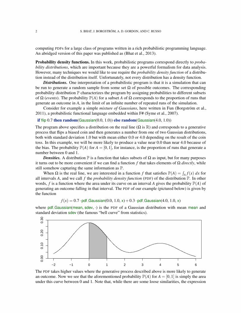
A f (x) dx forall intervals A, and we call f the probability density function (PDF) of the distribution P. In otherwords, f is a function where the area under its curve on an interval A gives the probability P(A) ofgenerating an outcome falling in that interval. The PDF of our example (pictured below) is given bythe function
f (x) = 0.7 ·pdf Gaussian(0.0, 1.0, x)+0.3 ·pdf Gaussian(4.0, 1.0, x)
where pdf Gaussian(mean, sdev, ·) is the PDF of a Gaussian distribution with mean mean andstandard deviation sdev (the famous “bell curve” from statistics).
−2 0 2 4 6
0.00
0.10
0.20
0.30
−1 1 3 5
The PDF takes higher values where the generative process described above is more likely to generatean outcome. Now we see that the aforementioned probability P(A) for A = [0,1] is simply the areaunder this curve between 0 and 1. Note that, while there are some loose similarities, the expression
DERIVING PROBABILITY DENSITY FUNCTIONS 3
for the PDF is different from the expression comprising the source program. In more complicatedprograms, the correspondence with the PDF is even less obvious.
Non-existence. Sometimes a distribution does not have a PDF. For example, if we change theelse-clause in our example to return 4.0 directly, instead of drawing from a Gaussian with mean 4.0,we get the following probabilistic program, which does not have a PDF:
if flip 0.7 then random(Gaussian(0.0, 1.0)) else 4.0
In short, the problem is that there is a non-zero amount of probability mass located on a zero-widthinterval (the process now returns 4.0 with probability 0.3), but integrals on such intervals yield zero,so we would never find a function that could satisfy the properties of being a PDF.
It is not always obvious which program modifications ruin the property of having a PDF,especially for multivariate distributions (thus far we have only given univariate distributions asexamples). This can be a problem if one is innocently exploring different variations of the model.Details and examples are given by Bhat et al. (2012), who provide the theory for addressing thisproblem, which we extend and implement in this work.
The task of data analysis. So far we have detailed what PDFs are, but not why we want them. Wemotivate the desire by explaining one popular use-case of PDFs that arises when applying Bayesianlearning to data analysis.
In the previous examples, the programs specify fully-known probability distributions. Whilethere is indeed randomness in the probabilistic behavior of the samples they generate, the nature ofthis uncertainty is entirely known—we know the means and variances of the Gaussians, as well asthe bias between the two, thus we can characterize the random behavior.
In real-world analysis tasks, we rarely have this luxury. Instead, we are often in the position oftrying to figure out what the parameters should be, given the data we see. Thus, applications typicallydeal with parameterized models (families of distributions indexed by a parameter), and they try tolearn something about which distributions in that family best explain the observed data. For example,in the following, moG is a parameterized model, indexed by the parameter (mA,mB):
let moG (mA,mB) =if flip 0.7 then random(Gaussian(mA, 1.0)) else random(Gaussian(mB, 1.0))
It specifies an infinite number of distributions, one for each choice of mA and mB.Now, as a data analyst, we may be presented a dataset that is a sequence of numeric values, and
we may also have some domain-specific reason to believe that it can be well modelled as a biasedmixture of Gaussians as specified by moG1. We now face the task of figuring out which choices ofmA and mB are likely. Intuitively, if we see a clump of datapoints around 0.0, we might be inclined tobelieve that the mean of one of the Gaussians is 0.0. Note that this is a one-dimensional, probabilisticversion of the problem of clustering. The means are the cluster centroids.
Bayesian learning. Bayesian modelling formalizes this task by requiring the modeller to provide asinput a prior distribution over the parameters and a generating distribution over the data. These areused to construct a posterior distribution over the parameters as the output.
1Whether this is actually an appropriate modelling choice depends on whether it captures enough of the essence of thetrue, unknown data-generating process (i.e. Nature), and is an entirely separate discussion.
4 S. BHAT, J. BORGSTROM, A. D. GORDON, AND C. RUSSO
The prior distribution is a distribution over the possible values of the parameters and capturesour belief about what values they are likely to take, before having seen any data (to a Bayesian,“belief” is synonymous with “probability distribution”). The following is one possible prior:
let prior () =let mA = random(Uniform(−10.0, 10.0)) inlet mB = random(Uniform(−10.0, 10.0)) in(mA, mB)
This specifies that we are certain that the means lie between -10.0 and 10.0, but are otherwiseuncertain, and our uncertainty about each mean is uniformly distributed between -10.0 and 10.0. Thisis of course a very particular assertion and is hopefully informed by domain knowledge. In practice,in the absense of domain knowledge, we can select a prior that reflects our open-mindedness aboutwhich values the means can take, such as a pair of Gaussians with a high standard deviation. Theprior produces a distribution over pairs of means as output, rather than taking a pair of means as aninput, as moG does.
The generating distribution is a model of how we believe Nature is generating a dataset given aspecific choice of the parameter. In our example this is given by moG together with
let gen n (mA,mB) = [| for i in 1 .. n→moG (mA,mB) |]This specifies a (parameterized) model for a dataset that is generated as an array of n independentand identically distributed (i.i.d.) values generated by moG.
The posterior distribution is a distribution over the possible values of the parameters and capturesour belief about what values they are likely to take, after seeing the data. The posterior is related tothe prior and generating distributions by Bayes’ rule, which gives us a way to describe how the prioris updated with the observed data to yield the posterior. Intuitively, this update represents the factthat our understanding about the world (our belief about the parameters) evolves based on the datawe see. Bishop provides an excellent account of Bayesian learning (Bishop, 2006).
Use-case of PDFs: Bayesian inference with MCMC. Unfortunately, while prior distributions andgenerating distributions are often straightforward to work with (we have control over them as themodeller), the posterior distributions often end up intractable or unwieldy to work with (Bayes’ ruledictates their form).
Markov chain Monte Carlo (MCMC) methods are one class of techniques that let us actually dosomething productive with the posterior distribution—MCMC can be used to generate samples fromthe posterior distribution. The idea of MCMC is to construct a Markov chain in the parameter space ofthe model, whose equilibrium distribution is the posterior distribution over model parameters. Neal(1993) gives an excellent review of MCMC methods. Here we use Filzbach (Purves and Lyutsarev,2012), an adaptive MCMC sampler based on the Metropolis-Hastings algorithm. All that is requiredfor such algorithms is the ability to calculate the posterior density given a set of parameters, upto proportion. The posterior does not need to be from a mathematically convenient family ofdistributions. Samples from the posterior can then serve as its representation, or be used to calculatemarginal distributions of parameters or other integrals under the posterior distribution.
DERIVING PROBABILITY DENSITY FUNCTIONS 5
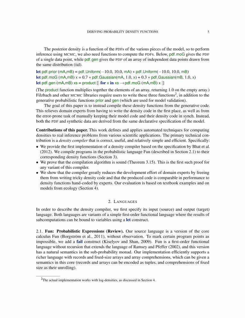
The posterior density is a function of the PDFs of the various pieces of the model, so to performinference using MCMC, we also need functions to compute the PDFs. Below, pdf moG gives the PDFof a single data point, while pdf gen gives the PDF of an array of independent data points drawn fromthe same distribution (iid).
let pdf prior (mA,mB) = pdf Uniform(−10.0, 10.0, mA) ∗ pdf Uniform(−10.0, 10.0, mB)let pdf moG (mA,mB) x = 0.7 ∗ pdf Gaussian(mA, 1.0, x) + 0.3 ∗ pdf Gaussian(mB, 1.0, x)let pdf gen (mA,mB) xs = product [| for x in xs→pdf moG (mA,mB) x |](The product function multiplies together the elements of an array, returning 1.0 on the empty array.)Filzbach and other MCMC libraries require users to write these three functions2, in addition to thegenerative probabilistic functions prior and gen (which are used for model validation).
The goal of this paper is to instead compile these density functions from the generative code.This relieves domain experts from having to write the density code in the first place, as well as fromthe error-prone task of manually keeping their model code and their density code in synch. Instead,both the PDF and synthetic data are derived from the same declarative specification of the model.
Contributions of this paper. This work defines and applies automated techniques for computingdensities to real inference problems from various scientific applications. The primary technical con-tribution is a density compiler that is correct, useful, and relatively simple and efficient. Specifically:• We provide the first implementation of a density compiler based on the specification by Bhat et al.
(2012). We compile programs in the probabilistic language Fun (described in Section 2.1) to theircorresponding density functions (Section 3).• We prove that the compilation algorithm is sound (Theorem 3.15). This is the first such proof for
any variant of this compiler.• We show that the compiler greatly reduces the development effort of domain experts by freeing
them from writing tricky density code and that the produced code is comparable in performance todensity functions hand-coded by experts. Our evaluation is based on textbook examples and onmodels from ecology (Section 4).
2. LANGUAGES
In order to describe the density compiler, we first specify its input (source) and output (target)language. Both languages are variants of a simple first-order functional language where the results ofsubcomputations can be bound to variables using a let construct.
2.1. Fun: Probabilistic Expressions (Review). Our source language is a version of the corecalculus Fun (Borgstrom et al., 2011), without observation. To mark certain program points asimpossible, we add a fail construct (Kiselyov and Shan, 2009). Fun is a first-order functionallanguage without recursion that extends the language of Ramsey and Pfeffer (2002), and this versionhas a natural semantics in the sub-probability monad. Our implementation efficiently supports aricher language with records and fixed-size arrays and array comprehensions, which can be given asemantics in this core (records and arrays can be encoded as tuples, and comprehensions of fixedsize as their unrolling).
2The actual implementation works with log-densities, as discussed in Section 4.
6 S. BHAT, J. BORGSTROM, A. D. GORDON, AND C. RUSSO
2.1.1. Syntax and Types of Fun: The language Fun has base types int, real and unit, product types(denoting pairs), and sum types (denoting tagged unions). A type is said to be discrete if it does notcontain real. We let c range over constant data of base type, n over integers and r over real numbers.We write ty(c) = t to mean that constant c has type t.Types of Fun:
t,u ::= int | real | unit | (t1 ∗ t2) | (t1 + t2)
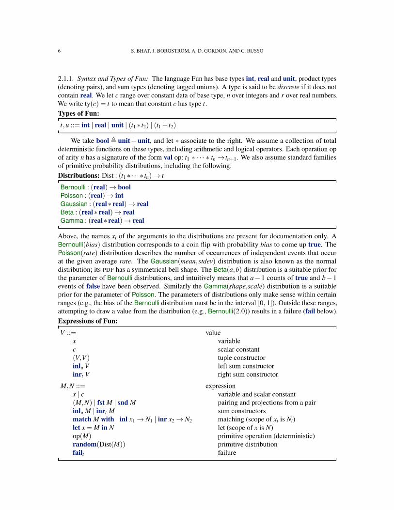
We take bool , unit+unit, and let ∗ associate to the right. We assume a collection of totaldeterministic functions on these types, including arithmetic and logical operators. Each operation opof arity n has a signature of the form val op: t1 ∗ · · · ∗ tn→ tn+1. We also assume standard familiesof primitive probability distributions, including the following.Distributions: Dist : (t1 ∗ · · · ∗ tn)→ t
Bernoulli : (real)→ boolPoisson : (real)→ intGaussian : (real∗ real)→ realBeta : (real∗ real)→ realGamma : (real∗ real)→ real
Above, the names xi of the arguments to the distributions are present for documentation only. ABernoulli(bias) distribution corresponds to a coin flip with probability bias to come up true. ThePoisson(rate) distribution describes the number of occurrences of independent events that occurat the given average rate. The Gaussian(mean,stdev) distribution is also known as the normaldistribution; its PDF has a symmetrical bell shape. The Beta(a,b) distribution is a suitable prior forthe parameter of Bernoulli distributions, and intuitively means that a−1 counts of true and b−1events of false have been observed. Similarly the Gamma(shape,scale) distribution is a suitableprior for the parameter of Poisson. The parameters of distributions only make sense within certainranges (e.g., the bias of the Bernoulli distribution must be in the interval [0, 1]). Outside these ranges,attempting to draw a value from the distribution (e.g., Bernoulli(2.0)) results in a failure (fail below).Expressions of Fun:
V ::= valuex variablec scalar constant(V,V ) tuple constructorinlu V left sum constructorinrt V right sum constructor
M,N ::= expressionx | c variable and scalar constant(M,N) | fst M | snd M pairing and projections from a pairinlu M | inrt M sum constructorsmatch M with inl x1→ N1 | inr x2→ N2 matching (scope of xi is Ni)let x = M in N let (scope of x is N)op(M) primitive operation (deterministic)random(Dist(M)) primitive distributionfailt failure
DERIVING PROBABILITY DENSITY FUNCTIONS 7
The let and match statements bind their variables (x,x1,x2); we identify expressions up to alpha-renaming of bound variables. Above, inl (resp. inr) generates a value corresponding to the left(resp. right) branch of a sum type. Values of sum type are deconstructed by the match construct,which behaves as either the left (N1) or the right (N2) branch depending on the result of M.
To ensure that a program has at most one type in a given typing environment, inl and inr areannotated with a type (see (FUN INL) below). The expression fail is annotated with the type it isused at. These types are included only for the convenience of our technical development, and canusually be inferred given a typable source program: we omit these types where they are not used. ()is the unit constant.
A source language term M is pure, written “M pure”, iff M does not contain any occurrence ofrandom or fail.
We write Uniform for Beta(1.0,1.0). In the binders of let and match expressions, we letstand for a variable that does not appear free in the scope of the binder. We make use of stan-dard sugar for let, such as writing M;N for let = M in N. We write if M then N1 else N2 formatch M with inl → N1 | inr → N2; this is most commonly used when M is Boolean. We let thetuple (M1,M2, . . . ,Mn) stand for (M1,(M2, . . . ,Mn)). Similarly, we write let x1,x2, . . . ,xn =V in Nfor let x1 = fst V in let z = snd V in let x2, . . . ,xn = z in N when z ] N.
When X is a term from some language (possibly with binders), we write x1, . . . ,xn ] X if none ofthe xi appear free in X .
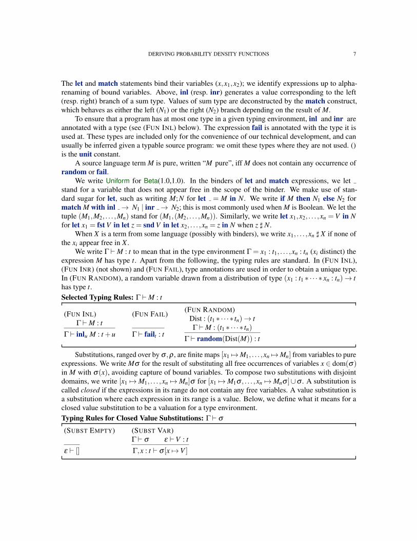
We write Γ `M : t to mean that in the type environment Γ = x1 : t1, . . . ,xn : tn (xi distinct) theexpression M has type t. Apart from the following, the typing rules are standard. In (FUN INL),(FUN INR) (not shown) and (FUN FAIL), type annotations are used in order to obtain a unique type.In (FUN RANDOM), a random variable drawn from a distribution of type (x1 : t1 ∗ · · · ∗ xn : tn)→ thas type t.Selected Typing Rules: Γ `M : t
(FUN INL)Γ `M : t
Γ ` inlu M : t +u
(FUN FAIL)
Γ ` failt : t
(FUN RANDOM)Dist : (t1 ∗ · · · ∗ tn)→ tΓ `M : (t1 ∗ · · · ∗ tn)
Γ ` random(Dist(M)) : t
Substitutions, ranged over by σ ,ρ , are finite maps [x1 7→M1, . . . ,xn 7→Mn] from variables to pureexpressions. We write Mσ for the result of substituting all free occurrences of variables x ∈ dom(σ)in M with σ(x), avoiding capture of bound variables. To compose two substitutions with disjointdomains, we write [x1 7→M1, . . . ,xn 7→Mn]σ for [x1 7→M1σ , . . . ,xn 7→Mnσ ]∪σ . A substitution iscalled closed if the expressions in its range do not contain any free variables. A value substitution isa substitution where each expression in its range is a value. Below, we define what it means for aclosed value substitution to be a valuation for a type environment.Typing Rules for Closed Value Substitutions: Γ ` σ
(SUBST EMPTY)
ε ` []
(SUBST VAR)Γ ` σ ε `V : t
Γ,x : t ` σ [x 7→V ]
8 S. BHAT, J. BORGSTROM, A. D. GORDON, AND C. RUSSO
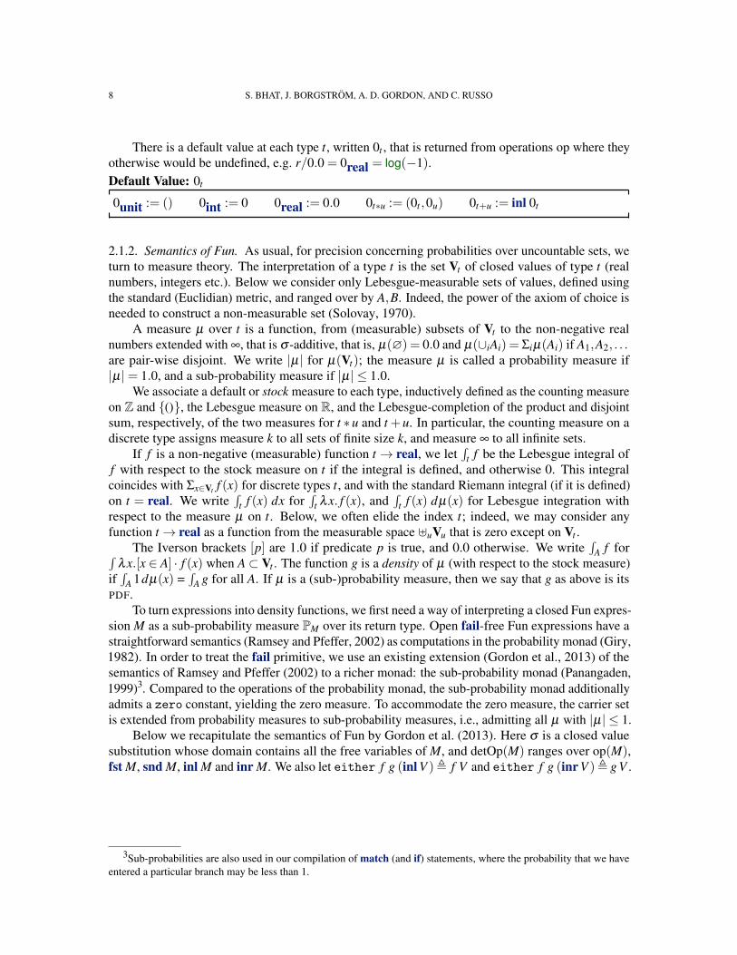
There is a default value at each type t, written 0t , that is returned from operations op where theyotherwise would be undefined, e.g. r/0.0 = 0real = log(−1).Default Value: 0t
0unit := () 0int := 0 0real := 0.0 0t∗u := (0t ,0u) 0t+u := inl 0t
2.1.2. Semantics of Fun. As usual, for precision concerning probabilities over uncountable sets, weturn to measure theory. The interpretation of a type t is the set Vt of closed values of type t (realnumbers, integers etc.). Below we consider only Lebesgue-measurable sets of values, defined usingthe standard (Euclidian) metric, and ranged over by A,B. Indeed, the power of the axiom of choice isneeded to construct a non-measurable set (Solovay, 1970).
A measure µ over t is a function, from (measurable) subsets of Vt to the non-negative realnumbers extended with ∞, that is σ -additive, that is, µ(∅) = 0.0 and µ(∪iAi) = Σiµ(Ai) if A1,A2, . . .are pair-wise disjoint. We write |µ| for µ(Vt); the measure µ is called a probability measure if|µ|= 1.0, and a sub-probability measure if |µ| ≤ 1.0.
We associate a default or stock measure to each type, inductively defined as the counting measureon Z and (), the Lebesgue measure on R, and the Lebesgue-completion of the product and disjointsum, respectively, of the two measures for t ∗u and t +u. In particular, the counting measure on adiscrete type assigns measure k to all sets of finite size k, and measure ∞ to all infinite sets.
If f is a non-negative (measurable) function t → real, we let∫
t f be the Lebesgue integral off with respect to the stock measure on t if the integral is defined, and otherwise 0. This integralcoincides with Σx∈Vt f (x) for discrete types t, and with the standard Riemann integral (if it is defined)on t = real. We write
∫t f (x) dx for
∫t λx. f (x), and
∫t f (x) dµ(x) for Lebesgue integration with
respect to the measure µ on t. Below, we often elide the index t; indeed, we may consider anyfunction t→ real as a function from the measurable space ]uVu that is zero except on Vt .
The Iverson brackets [p] are 1.0 if predicate p is true, and 0.0 otherwise. We write∫
A f for∫λx.[x ∈ A] · f (x) when A⊂ Vt . The function g is a density of µ (with respect to the stock measure)
if∫
A 1dµ(x) =∫
A g for all A. If µ is a (sub-)probability measure, then we say that g as above is itsPDF.
To turn expressions into density functions, we first need a way of interpreting a closed Fun expres-sion M as a sub-probability measure PM over its return type. Open fail-free Fun expressions have astraightforward semantics (Ramsey and Pfeffer, 2002) as computations in the probability monad (Giry,1982). In order to treat the fail primitive, we use an existing extension (Gordon et al., 2013) of thesemantics of Ramsey and Pfeffer (2002) to a richer monad: the sub-probability monad (Panangaden,1999)3. Compared to the operations of the probability monad, the sub-probability monad additionallyadmits a zero constant, yielding the zero measure. To accommodate the zero measure, the carrier setis extended from probability measures to sub-probability measures, i.e., admitting all µ with |µ| ≤ 1.
Below we recapitulate the semantics of Fun by Gordon et al. (2013). Here σ is a closed valuesubstitution whose domain contains all the free variables of M, and detOp(M) ranges over op(M),fst M, snd M, inl M and inr M. We also let either f g (inl V ), f V and either f g (inr V ), g V .
3Sub-probabilities are also used in our compilation of match (and if) statements, where the probability that we haveentered a particular branch may be less than 1.
DERIVING PROBABILITY DENSITY FUNCTIONS 9
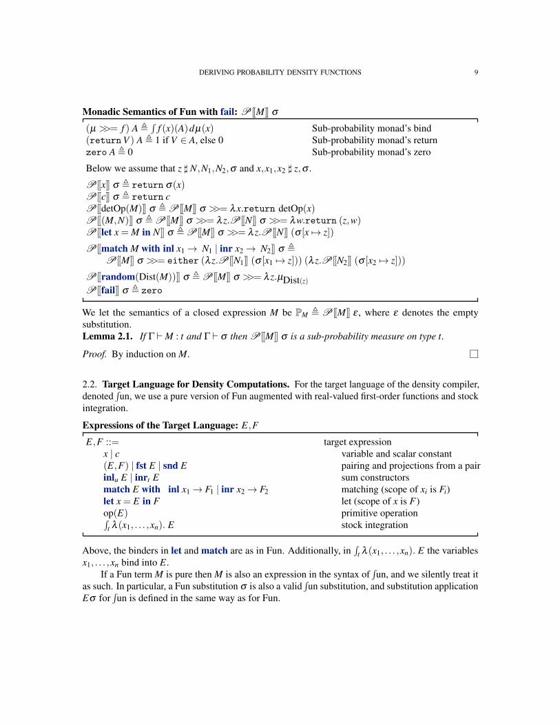
Monadic Semantics of Fun with fail: P[[M]] σ
(µ >>= f ) A ,∫
f (x)(A)dµ(x) Sub-probability monad’s bind(returnV ) A , 1 if V ∈ A, else 0 Sub-probability monad’s returnzero A , 0 Sub-probability monad’s zero
Below we assume that z ] N,N1,N2,σ and x,x1,x2 ] z,σ .
P[[x]] σ , return σ(x)P[[c]] σ , return cP[[detOp(M)]] σ , P[[M]] σ >>= λx.return detOp(x)P[[(M,N)]] σ , P[[M]] σ >>= λ z.P[[N]] σ >>= λw.return (z,w)P[[let x = M in N]] σ , P[[M]] σ >>= λ z.P[[N]] (σ [x 7→ z])
P[[match M with inl x1→ N1 | inr x2→ N2]] σ ,P[[M]] σ >>= either (λ z.P[[N1]] (σ [x1 7→ z])) (λ z.P[[N2]] (σ [x2 7→ z]))
P[[random(Dist(M))]] σ , P[[M]] σ >>= λ z.µDist(z)P[[fail]] σ , zero
We let the semantics of a closed expression M be PM , P[[M]] ε , where ε denotes the emptysubstitution.Lemma 2.1. If Γ `M : t and Γ ` σ then P[[M]] σ is a sub-probability measure on type t.
Proof. By induction on M.
2.2. Target Language for Density Computations. For the target language of the density compiler,denoted
∫un, we use a pure version of Fun augmented with real-valued first-order functions and stock
integration.
Expressions of the Target Language: E,F
E,F ::= target expressionx | c variable and scalar constant(E,F) | fst E | snd E pairing and projections from a pairinlu E | inrt E sum constructorsmatch E with inl x1→ F1 | inr x2→ F2 matching (scope of xi is Fi)let x = E in F let (scope of x is F)op(E) primitive operation∫
t λ (x1, . . . ,xn). E stock integration
Above, the binders in let and match are as in Fun. Additionally, in∫
t λ (x1, . . . ,xn). E the variablesx1, . . . ,xn bind into E.
If a Fun term M is pure then M is also an expression in the syntax of∫un, and we silently treat it
as such. In particular, a Fun substitution σ is also a valid∫un substitution, and substitution application
Eσ for∫un is defined in the same way as for Fun.
10 S. BHAT, J. BORGSTROM, A. D. GORDON, AND C. RUSSO
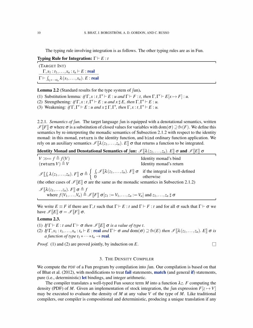
The typing rule involving integration is as follows. The other typing rules are as in Fun.
Typing Rule for Integration: Γ ` E : t
(TARGET INT)Γ,x1 : t1, . . . ,xn : tn ` E : real
Γ `∫
t1∗···∗tn λ (x1, . . . ,xn). E : real
Lemma 2.2 (Standard results for the type system of∫un).
(1) Substitution lemma: if Γ,x : t,Γ′ ` E : u and Γ ` F : t, then Γ,Γ′ ` E[x 7→ F ] : u.(2) Strengthening: if Γ,x : t,Γ′ ` E : u and x ] E, then Γ,Γ′ ` E : u.(3) Weakening: if Γ,Γ′ ` E : u and x ] Γ,Γ′, then Γ,x : t,Γ′ ` E : u.
2.2.1. Semantics of∫un. The target language
∫un is equipped with a denotational semantics, written
I [[F ]]σ where σ is a substitution of closed values for variables with dom(σ)⊇ fv(F). We define thissemantics by re-interpreting the monadic semantics of Subsection 2.1.2 with respect to the identitymonad: in this monad, return is the identity function, and bind ordinary function application. Werely on an auxiliary semantics I [[λ (z1, . . . ,zn). E]] σ that returns a function to be integrated.
Identity Monad and Denotational Semantics of∫un: I [[λ (z1, . . . ,zn). E]] σ and I [[E]] σ
V >>= f , f (V ) Identity monad’s bind(returnV ),V Identity monad’s return
I [[∫
t λ (z1, . . . ,zn). F ]] σ ,
∫t I [[λ (z1, . . . ,zn). F ]] σ if the integral is well-defined
0 otherwise(the other cases of I [[E]] σ are the same as the monadic semantics in Subsection 2.1.2)
I [[λ (z1, . . . ,zn). F ]] σ , fwhere f (V1, . . . ,Vn), I [[F ]] σ [z1 :=V1, . . . ,zn :=Vn] and z1, . . . ,zn ] σ
We write E ≡ F if there are Γ, t such that Γ ` E : t and Γ ` F : t and for all σ such that Γ ` σ wehave I [[E]] σ = I [[F ]] σ .
Lemma 2.3.(1) If Γ ` E : t and Γ ` σ then I [[E]] σ is a value of type t.(2) If Γ,x1 : t1, . . . ,xn : tn ` E : real and Γ ` σ and dom(σ)⊇ fv(E) then I [[λ (z1, . . . ,zn). E]] σ is
a function of type t1 ∗ · · · ∗ tn→ real.
Proof. (1) and (2) are proved jointly, by induction on E.
3. THE DENSITY COMPILER
We compute the PDF of a Fun program by compilation into∫un. Our compilation is based on that
of Bhat et al. (2012), with modifications to treat fail statements, match (and general if) statements,pure (i.e., deterministic) let bindings, and integer arithmetic.
The compiler translates a well-typed Fun source term M into a function λ z. F computing thedensity (PDF) of M. Given an implementation of stock integration, the
∫un expression F [z 7→ V ]
may be executed to evaluate the density of M at any value V of the type of M. Like traditionalcompilers, our compiler is compositional and deterministic, producing a unique translation if any
DERIVING PROBABILITY DENSITY FUNCTIONS 11
at all (Lemma 3.13). Unlike traditional compilers, our compiler is partial and will fail to produce atranslation for some well-typed source terms. In particular, if M does not have a density function thenthe compiler will fail to produce an F . However, it may also fail if M has a PDF, but the compiler isjust not complete enough to compute it. In particular, let-bound expressions must either be pure orhave a PDF, even if their result is not used. The correctness statement for the compiler is given byTheorem 3.15.
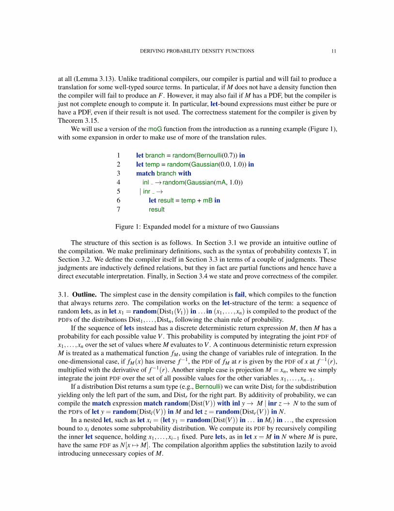
We will use a version of the moG function from the introduction as a running example (Figure 1),with some expansion in order to make use of more of the translation rules.
1 let branch = random(Bernoulli(0.7)) in2 let temp = random(Gaussian(0.0, 1.0)) in3 match branch with4 inl → random(Gaussian(mA, 1.0))5 | inr →6 let result = temp + mB in7 result
Figure 1: Expanded model for a mixture of two Gaussians
The structure of this section is as follows. In Section 3.1 we provide an intuitive outline ofthe compilation. We make preliminary definitions, such as the syntax of probability contexts ϒ, inSection 3.2. We define the compiler itself in Section 3.3 in terms of a couple of judgments. Thesejudgments are inductively defined relations, but they in fact are partial functions and hence have adirect executable interpretation. Finally, in Section 3.4 we state and prove correctness of the compiler.
3.1. Outline. The simplest case in the density compilation is fail, which compiles to the functionthat always returns zero. The compilation works on the let-structure of the term: a sequence ofrandom lets, as in let x1 = random(Dist1(V1)) in . . . in (x1, . . . ,xn) is compiled to the product of thePDFs of the distributions Dist1, . . . ,Distn, following the chain rule of probability.
If the sequence of lets instead has a discrete deterministic return expression M, then M has aprobability for each possible value V . This probability is computed by integrating the joint PDF ofx1, . . . ,xn over the set of values where M evaluates to V . A continuous deterministic return expressionM is treated as a mathematical function fM, using the change of variables rule of integration. In theone-dimensional case, if fM(x) has inverse f−1, the PDF of fM at r is given by the PDF of x at f−1(r),multiplied with the derivative of f−1(r). Another simple case is projection M = xn, where we simplyintegrate the joint PDF over the set of all possible values for the other variables x1, . . . ,xn−1.
If a distribution Dist returns a sum type (e.g., Bernoulli) we can write Distl for the subdistributionyielding only the left part of the sum, and Distr for the right part. By additivity of probability, we cancompile the match expression match random(Dist(V )) with inl y→ M | inr z→ N to the sum ofthe PDFs of let y = random(Distl(V )) in M and let z = random(Distr(V )) in N.
In a nested let, such as let xi = (let y1 = random(Dist(V )) in . . . in Mi) in . . ., the expressionbound to xi denotes some subprobability distribution. We compute its PDF by recursively compilingthe inner let sequence, holding x1, . . . ,xi−1 fixed. Pure lets, as in let x = M in N where M is pure,have the same PDF as N[x 7→M]. The compilation algorithm applies the substitution lazily to avoidintroducing unnecessary copies of M.
12 S. BHAT, J. BORGSTROM, A. D. GORDON, AND C. RUSSO
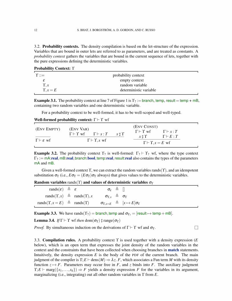
3.2. Probability contexts. The density compilation is based on the let-structure of the expression.Variables that are bound in outer lets are referred to as parameters, and are treated as constants. Aprobability context gathers the variables that are bound in the current sequence of lets, together withthe pure expressions defining the deterministic variables.
Probability Context: ϒ
ϒ ::= probability contextε empty contextϒ,x random variableϒ,x = E deterministic variable
Example 3.1. The probability context at line 7 of Figure 1 is ϒ7 := branch, temp, result= temp + mB,containing two random variables and one deterministic variable.
For a probability context to be well-formed, it has to be well-scoped and well-typed.
Well-formed probability context: Γ ` ϒ wf
(ENV EMPTY)
Γ ` ε wf
(ENV VAR)Γ ` ϒ wf Γ ` x : T x ] ϒ
Γ ` ϒ,x wf
(ENV CONST)Γ ` ϒ wf Γ ` x : T
x ] ϒ Γ ` E : T
Γ ` ϒ,x = E wf
Example 3.2. The probability context ϒ7 is well-formed: Γ7 ` ϒ7 wf, where the type contextΓ7 := mA:real,mB:real,branch:bool, temp:real, result:real also contains the types of the parametersmA and mB.
Given a well-formed context ϒ, we can extract the random variables rands(ϒ), and an idempotentsubstitution σϒ (i.e., Eσϒ = (Eσϒ)σϒ always) that gives values to the deterministic variables.
Random variables rands(ϒ) and values of deterministic variables σϒ
rands(ε) , ε σε , []
rands(ϒ,x) , rands(ϒ),x σϒ,x , σϒ
rands(ϒ,x = E) , rands(ϒ) σϒ,x=E , [x 7→ E]σϒ
Example 3.3. We have rands(ϒ7) = branch, temp and σϒ7 = [result 7→ temp+mB].
Lemma 3.4. If Γ ` ϒ wf then dom(σϒ) ] range(σϒ)
Proof. By simultaneous induction on the derivations of Γ ` ϒ wf and σϒ.
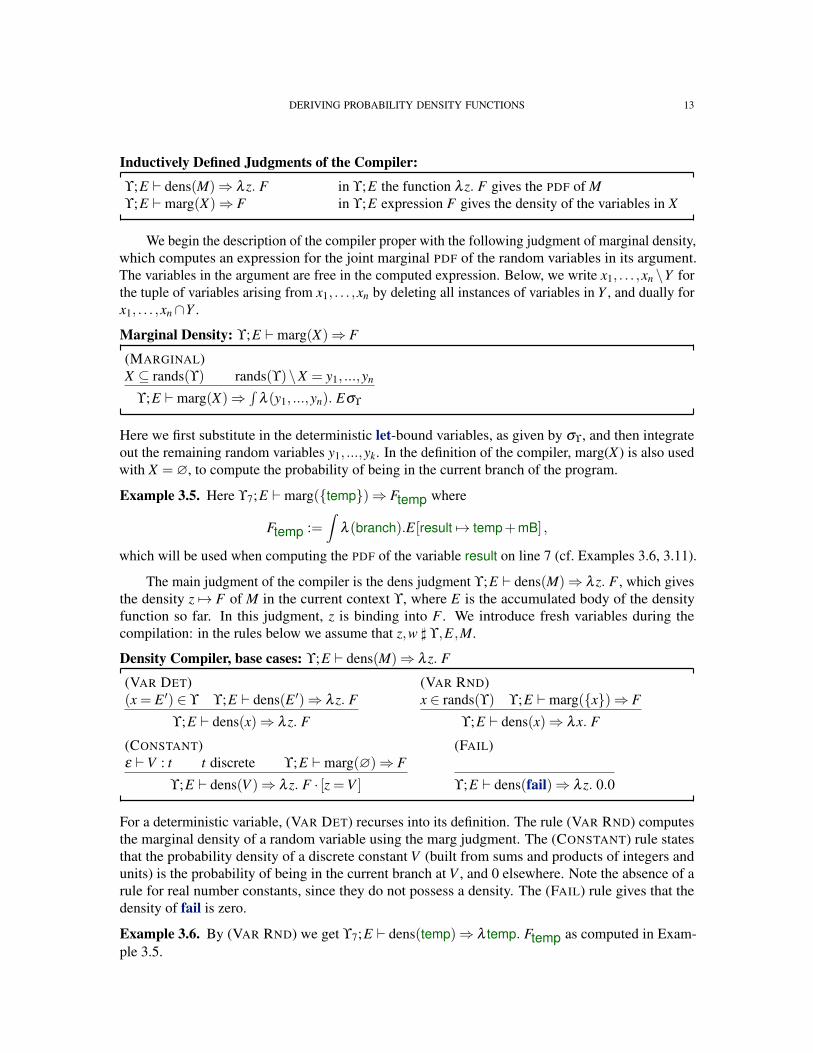
3.3. Compilation rules. A probability context ϒ is used together with a density expression (Ebelow), which is an open term that expresses the joint density of the random variables in thecontext and the constraints that have been collected when choosing branches in match statements.Intuitively, the density expression E is the body of the PDF of the current branch. The mainjudgment of the compiler is ϒ;E ` dens(M)⇒ λ z. F , which associates a Fun term M with its densityfunction z 7→ F . Parameters may occur free in F , and z binds into F . The auxiliary judgmentϒ;E ` marg(x1, . . . ,xk)⇒ F yields a density expression F for the variables in its argument,marginalizing (i.e., integrating) out all other random variables in ϒ from E.
DERIVING PROBABILITY DENSITY FUNCTIONS 13
Inductively Defined Judgments of the Compiler:
ϒ;E ` dens(M)⇒ λ z. F in ϒ;E the function λ z. F gives the PDF of Mϒ;E `marg(X)⇒ F in ϒ;E expression F gives the density of the variables in X
We begin the description of the compiler proper with the following judgment of marginal density,which computes an expression for the joint marginal PDF of the random variables in its argument.The variables in the argument are free in the computed expression. Below, we write x1, . . . ,xn \Y forthe tuple of variables arising from x1, . . . ,xn by deleting all instances of variables in Y , and dually forx1, . . . ,xn∩Y .
Marginal Density: ϒ;E `marg(X)⇒ F
(MARGINAL)X ⊆ rands(ϒ) rands(ϒ)\X = y1, ...,yn
ϒ;E `marg(X)⇒∫
λ (y1, ...,yn). Eσϒ
Here we first substitute in the deterministic let-bound variables, as given by σϒ, and then integrateout the remaining random variables y1, ...,yk. In the definition of the compiler, marg(X) is also usedwith X =∅, to compute the probability of being in the current branch of the program.
Example 3.5. Here ϒ7;E `marg(temp)⇒ Ftemp where
Ftemp :=∫
λ (branch).E[result 7→ temp+mB] ,
which will be used when computing the PDF of the variable result on line 7 (cf. Examples 3.6, 3.11).
The main judgment of the compiler is the dens judgment ϒ;E ` dens(M)⇒ λ z. F , which givesthe density z 7→ F of M in the current context ϒ, where E is the accumulated body of the densityfunction so far. In this judgment, z is binding into F . We introduce fresh variables during thecompilation: in the rules below we assume that z,w ] ϒ,E,M.
Density Compiler, base cases: ϒ;E ` dens(M)⇒ λ z. F
(VAR DET)(x = E ′) ∈ ϒ ϒ;E ` dens(E ′)⇒ λ z. F
ϒ;E ` dens(x)⇒ λ z. F
(VAR RND)x ∈ rands(ϒ) ϒ;E `marg(x)⇒ F
ϒ;E ` dens(x)⇒ λx. F
(CONSTANT)ε `V : t t discrete ϒ;E `marg(∅)⇒ F
ϒ;E ` dens(V )⇒ λ z. F · [z =V ]
(FAIL)
ϒ;E ` dens(fail)⇒ λ z. 0.0
For a deterministic variable, (VAR DET) recurses into its definition. The rule (VAR RND) computesthe marginal density of a random variable using the marg judgment. The (CONSTANT) rule statesthat the probability density of a discrete constant V (built from sums and products of integers andunits) is the probability of being in the current branch at V , and 0 elsewhere. Note the absence of arule for real number constants, since they do not possess a density. The (FAIL) rule gives that thedensity of fail is zero.
Example 3.6. By (VAR RND) we get ϒ7;E ` dens(temp)⇒ λ temp. Ftemp as computed in Exam-ple 3.5.
14 S. BHAT, J. BORGSTROM, A. D. GORDON, AND C. RUSSO
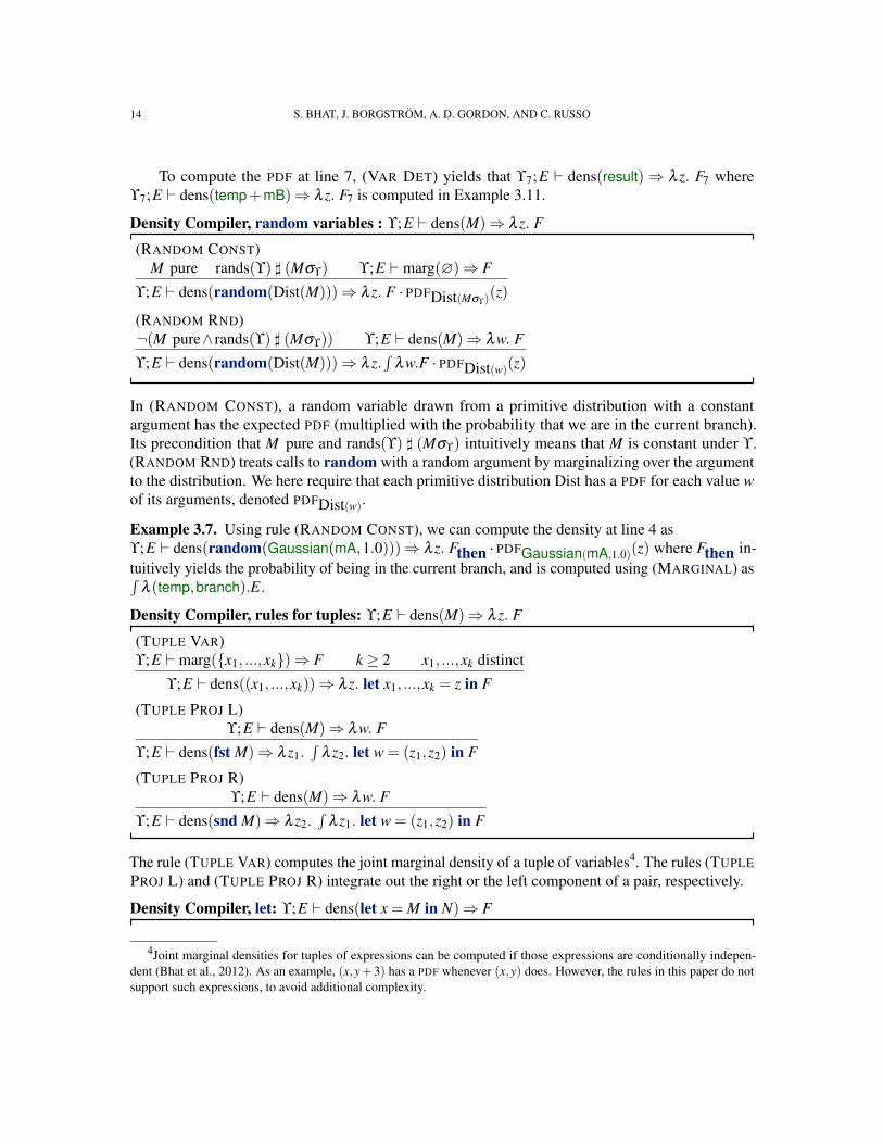
To compute the PDF at line 7, (VAR DET) yields that ϒ7;E ` dens(result)⇒ λ z. F7 whereϒ7;E ` dens(temp+mB)⇒ λ z. F7 is computed in Example 3.11.
Density Compiler, random variables : ϒ;E ` dens(M)⇒ λ z. F
(RANDOM CONST)M pure rands(ϒ) ] (Mσϒ) ϒ;E `marg(∅)⇒ F
ϒ;E ` dens(random(Dist(M)))⇒ λ z. F · PDFDist(Mσϒ)(z)
(RANDOM RND)¬(M pure∧ rands(ϒ) ] (Mσϒ)) ϒ;E ` dens(M)⇒ λw. F
ϒ;E ` dens(random(Dist(M)))⇒ λ z.∫
λw.F · PDFDist(w)(z)
In (RANDOM CONST), a random variable drawn from a primitive distribution with a constantargument has the expected PDF (multiplied with the probability that we are in the current branch).Its precondition that M pure and rands(ϒ) ] (Mσϒ) intuitively means that M is constant under ϒ.(RANDOM RND) treats calls to random with a random argument by marginalizing over the argumentto the distribution. We here require that each primitive distribution Dist has a PDF for each value wof its arguments, denoted PDFDist(w).
Example 3.7. Using rule (RANDOM CONST), we can compute the density at line 4 asϒ;E ` dens(random(Gaussian(mA,1.0)))⇒ λ z. Fthen · PDFGaussian(mA,1.0)(z) where Fthen in-tuitively yields the probability of being in the current branch, and is computed using (MARGINAL) as∫
λ (temp,branch).E.
Density Compiler, rules for tuples: ϒ;E ` dens(M)⇒ λ z. F
(TUPLE VAR)ϒ;E `marg(x1, ...,xk)⇒ F k ≥ 2 x1, ...,xk distinct
ϒ;E ` dens((x1, ...,xk))⇒ λ z. let x1, ...,xk = z in F
(TUPLE PROJ L)ϒ;E ` dens(M)⇒ λw. F
ϒ;E ` dens(fst M)⇒ λ z1.∫
λ z2. let w = (z1,z2) in F
(TUPLE PROJ R)ϒ;E ` dens(M)⇒ λw. F
ϒ;E ` dens(snd M)⇒ λ z2.∫
λ z1. let w = (z1,z2) in F
The rule (TUPLE VAR) computes the joint marginal density of a tuple of variables4. The rules (TUPLEPROJ L) and (TUPLE PROJ R) integrate out the right or the left component of a pair, respectively.
Density Compiler, let: ϒ;E ` dens(let x = M in N)⇒ F
4Joint marginal densities for tuples of expressions can be computed if those expressions are conditionally indepen-dent (Bhat et al., 2012). As an example, (x,y+3) has a PDF whenever (x,y) does. However, the rules in this paper do notsupport such expressions, to avoid additional complexity.
DERIVING PROBABILITY DENSITY FUNCTIONS 15
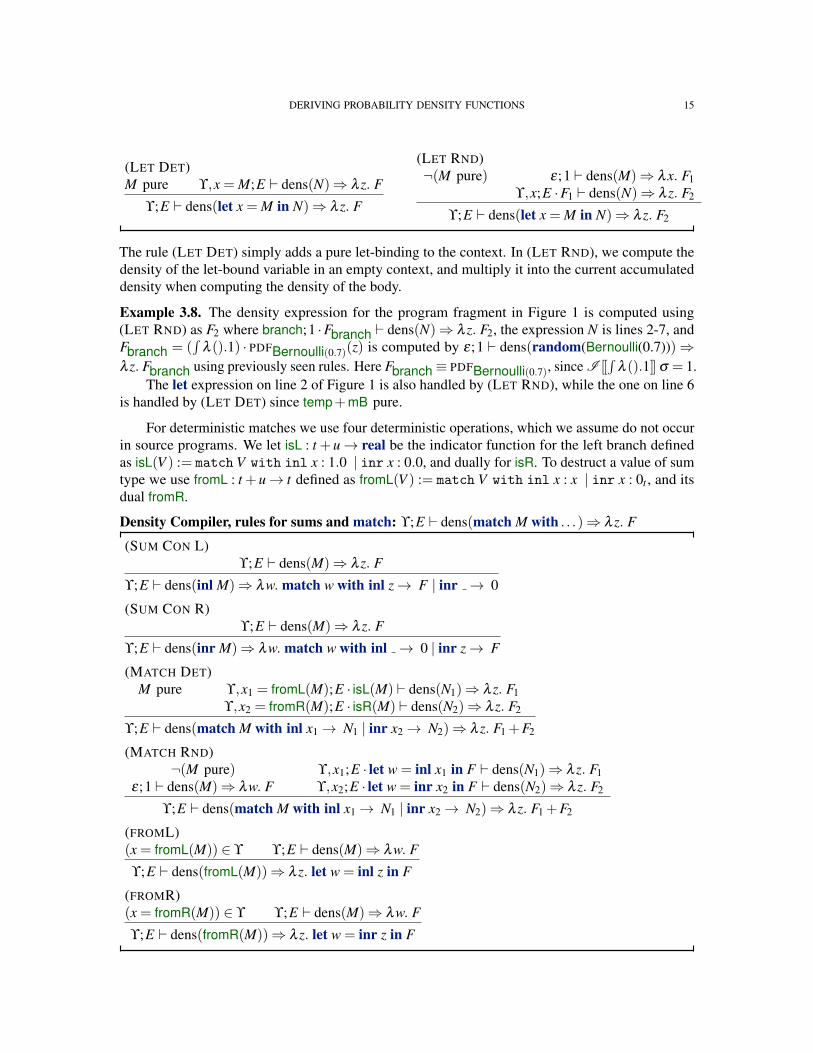
(LET DET)M pure ϒ,x = M;E ` dens(N)⇒ λ z. F
ϒ;E ` dens(let x = M in N)⇒ λ z. F
(LET RND)¬(M pure) ε;1 ` dens(M)⇒ λx. F1
ϒ,x;E ·F1 ` dens(N)⇒ λ z. F2
ϒ;E ` dens(let x = M in N)⇒ λ z. F2
The rule (LET DET) simply adds a pure let-binding to the context. In (LET RND), we compute thedensity of the let-bound variable in an empty context, and multiply it into the current accumulateddensity when computing the density of the body.
Example 3.8. The density expression for the program fragment in Figure 1 is computed using(LET RND) as F2 where branch;1 ·Fbranch ` dens(N)⇒ λ z. F2, the expression N is lines 2-7, andFbranch = (
∫λ ().1) · PDFBernoulli(0.7)(z) is computed by ε;1 ` dens(random(Bernoulli(0.7)))⇒
λ z. Fbranch using previously seen rules. Here Fbranch≡ PDFBernoulli(0.7), since I [[∫
λ ().1]] σ = 1.The let expression on line 2 of Figure 1 is also handled by (LET RND), while the one on line 6
is handled by (LET DET) since temp+mB pure.
For deterministic matches we use four deterministic operations, which we assume do not occurin source programs. We let isL : t +u→ real be the indicator function for the left branch definedas isL(V ) := match V with inl x : 1.0 | inr x : 0.0, and dually for isR. To destruct a value of sumtype we use fromL : t +u→ t defined as fromL(V ) := match V with inl x : x | inr x : 0t , and itsdual fromR.
Density Compiler, rules for sums and match: ϒ;E ` dens(match M with . . .)⇒ λ z. F
(SUM CON L)ϒ;E ` dens(M)⇒ λ z. F
ϒ;E ` dens(inl M)⇒ λw. match w with inl z→ F | inr → 0
(SUM CON R)ϒ;E ` dens(M)⇒ λ z. F
ϒ;E ` dens(inr M)⇒ λw. match w with inl → 0 | inr z→ F
(MATCH DET)M pure ϒ,x1 = fromL(M);E · isL(M) ` dens(N1)⇒ λ z. F1
ϒ,x2 = fromR(M);E · isR(M) ` dens(N2)⇒ λ z. F2
ϒ;E ` dens(match M with inl x1→ N1 | inr x2→ N2)⇒ λ z. F1 +F2
(MATCH RND)¬(M pure) ϒ,x1;E · let w = inl x1 in F ` dens(N1)⇒ λ z. F1
ε;1 ` dens(M)⇒ λw. F ϒ,x2;E · let w = inr x2 in F ` dens(N2)⇒ λ z. F2
ϒ;E ` dens(match M with inl x1→ N1 | inr x2→ N2)⇒ λ z. F1 +F2
(FROML)(x = fromL(M)) ∈ ϒ ϒ;E ` dens(M)⇒ λw. F
ϒ;E ` dens(fromL(M))⇒ λ z. let w = inl z in F
(FROMR)(x = fromR(M)) ∈ ϒ ϒ;E ` dens(M)⇒ λw. F
ϒ;E ` dens(fromR(M))⇒ λ z. let w = inr z in F

16 S. BHAT, J. BORGSTROM, A. D. GORDON, AND C. RUSSO
(SUM CON L) states that the density of inl M is the density of M in the left branch of asum, and 0 in the right. Its dual is (FROML). (MATCH DET) is based on (LET DET), and weadditionally multiply the constraint that we are in the correct branch (isL(M) or isR(M)) with thejoint density expression. We employ the functions fromL and fromR and their associated rules(FROML) and (FROMR) to avoid additional calls to (MATCH DET) arising from (VAR DET) if thecompilation of the density of Ni requires computing the density of the match-bound variable yi, as inmatch fst z with inl y1→ y1 | inr y2→ y2. Since we assume that fromL and fromR do not appearin source programs, these rules are only ever used in the case described above. The (MATCH RND)rule is based on (LET RND), and we again multiply in the constraint that we are in the left (or right)branch of the match.
Example 3.9. The match selector on line 3 is a pure expression, so rule (MATCH DET) applies. Forthe left branch, we let E4 ≡ PDFBernoulli(0.7)(branch) · PDFGaussian(0,1.0)(temp) · isL(branch) andϒ4 = branch, temp, = fromL(branch) and compute
ϒ4;E4 ` dens(random(Gaussian(mA, 1.0)))⇒ λ z. F4
where F4 is computed using (RANDOM CONST) and (MARGINAL) as(∫λ (branch, temp).E4
)·PDFGaussian(mA,1.0)(z)
Here I [[∫
λ (branch, temp).E4]] σ = 0.7, so the contribution of the left branch to the PDF of thematch is the PDF of the branch scaled by the probability of entering the left branch. In general, thisholds when the branch expression is independent from the body of the branch.
For the right branch, see Example 3.11. We then obtain the PDF of the match as the sum of thePDFs of the two branches.
Our implementation of the compiler uses the following derived rules for if statements where thebranching expression is of type bool, and does not treat other sum types nor matches.
Derived rules for if statements
(IF DET)M pure ϒ;E · isL(M) ` dens(N1)⇒ λ z. F1
ϒ;E · isR(M) ` dens(N2)⇒ λ z. F2
ϒ;E ` dens(if M then N1 else N2)⇒ λ z. F1 +F2
(IF RND)¬(M pure) ϒ;E · let w = true in F ` dens(N1)⇒ λ z. F1
ε;1 ` dens(M)⇒ λw. F ϒ;E · let w = false in F ` dens(N2)⇒ λ z. F2
ϒ;E ` dens(if M then N1 else N2)⇒ λ z. F1 +F2
Example 3.10. Since the match-bound variables (lines 4 and 5) do not appear in the bodies of thematch branches, we can instead use rule (IF DET) to avoid adding them to the probability contextwhen computing the PDF of the body (cf. Example 3.1).
Density compiler, discrete operations : ϒ;E ` dens( f (M))⇒ F
(DISCRETE)M pure ϒ;E `marg(x1, . . . ,xn)⇒ F f 6∈ fromL, fromR
f : t→ u u discrete rands(ϒ)∩ fv(Mσϒ) = x1, . . . ,xn
ϒ;E ` dens( f (M))⇒ λw.∫
λ (x1, . . . ,xn). F · [w = f (Mσϒ)]
DERIVING PROBABILITY DENSITY FUNCTIONS 17
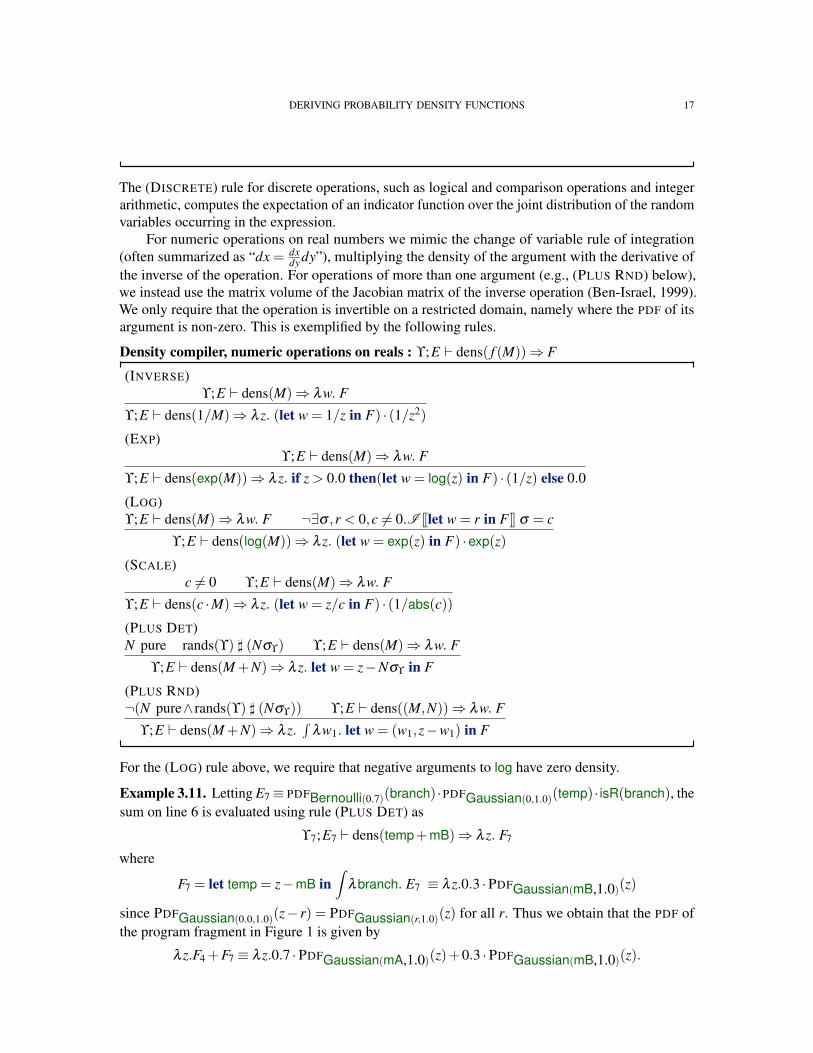
The (DISCRETE) rule for discrete operations, such as logical and comparison operations and integerarithmetic, computes the expectation of an indicator function over the joint distribution of the randomvariables occurring in the expression.
For numeric operations on real numbers we mimic the change of variable rule of integration(often summarized as “dx = dx
dy dy”), multiplying the density of the argument with the derivative ofthe inverse of the operation. For operations of more than one argument (e.g., (PLUS RND) below),we instead use the matrix volume of the Jacobian matrix of the inverse operation (Ben-Israel, 1999).We only require that the operation is invertible on a restricted domain, namely where the PDF of itsargument is non-zero. This is exemplified by the following rules.
Density compiler, numeric operations on reals : ϒ;E ` dens( f (M))⇒ F
(INVERSE)ϒ;E ` dens(M)⇒ λw. F
ϒ;E ` dens(1/M)⇒ λ z. (let w = 1/z in F) · (1/z2)
(EXP)ϒ;E ` dens(M)⇒ λw. F
ϒ;E ` dens(exp(M))⇒ λ z. if z > 0.0 then(let w = log(z) in F) · (1/z) else 0.0
(LOG)ϒ;E ` dens(M)⇒ λw. F ¬∃σ ,r < 0,c 6= 0.I [[let w = r in F ]] σ = c
ϒ;E ` dens(log(M))⇒ λ z. (let w = exp(z) in F) ·exp(z)
(SCALE)c 6= 0 ϒ;E ` dens(M)⇒ λw. F
ϒ;E ` dens(c ·M)⇒ λ z. (let w = z/c in F) · (1/abs(c))
(PLUS DET)N pure rands(ϒ) ] (Nσϒ) ϒ;E ` dens(M)⇒ λw. F
ϒ;E ` dens(M+N)⇒ λ z. let w = z−Nσϒ in F
(PLUS RND)¬(N pure∧ rands(ϒ) ] (Nσϒ)) ϒ;E ` dens((M,N))⇒ λw. F
ϒ;E ` dens(M+N)⇒ λ z.∫
λw1. let w = (w1,z−w1) in F
For the (LOG) rule above, we require that negative arguments to log have zero density.
Example 3.11. Letting E7≡ PDFBernoulli(0.7)(branch) ·PDFGaussian(0,1.0)(temp) · isR(branch), thesum on line 6 is evaluated using rule (PLUS DET) as
ϒ7;E7 ` dens(temp+mB)⇒ λ z. F7
where
F7 = let temp = z−mB in∫
λbranch. E7 ≡ λ z.0.3 ·PDFGaussian(mB,1.0)(z)
since PDFGaussian(0.0,1.0)(z− r) = PDFGaussian(r,1.0)(z) for all r. Thus we obtain that the PDF ofthe program fragment in Figure 1 is given by
λ z.F4 +F7 ≡ λ z.0.7 ·PDFGaussian(mA,1.0)(z)+0.3 ·PDFGaussian(mB,1.0)(z).
18 S. BHAT, J. BORGSTROM, A. D. GORDON, AND C. RUSSO
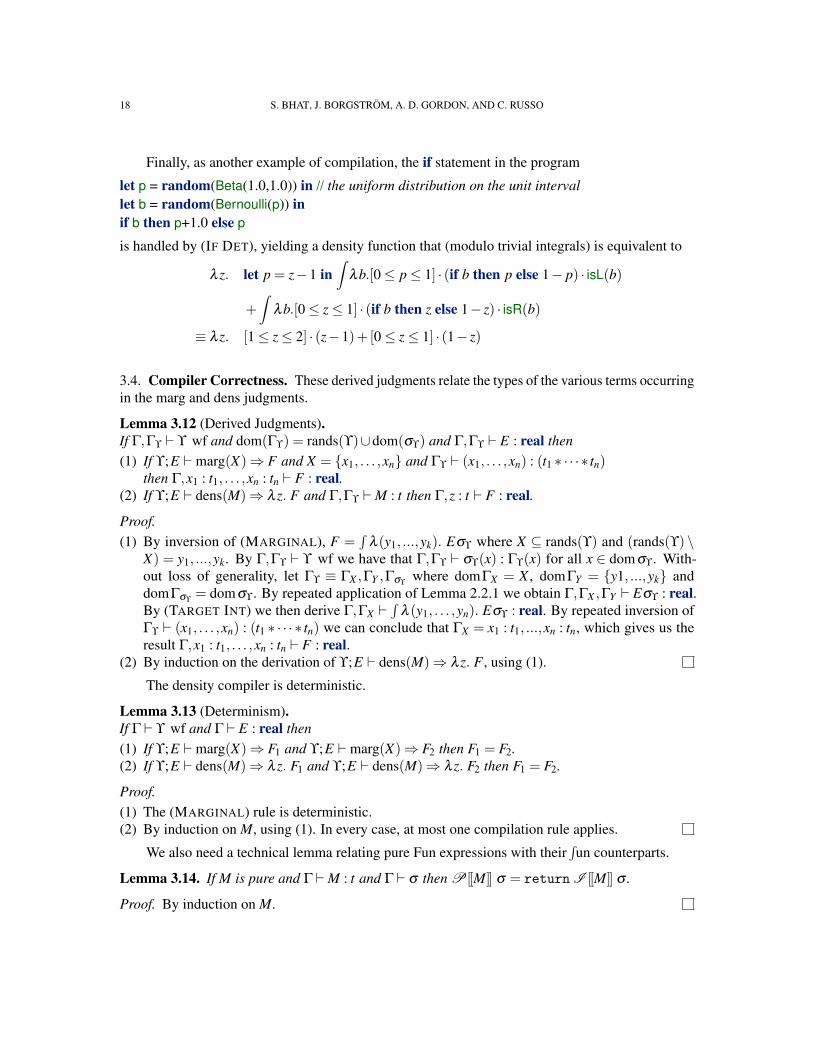
Finally, as another example of compilation, the if statement in the program
let p = random(Beta(1.0,1.0)) in // the uniform distribution on the unit intervallet b = random(Bernoulli(p)) inif b then p+1.0 else p
is handled by (IF DET), yielding a density function that (modulo trivial integrals) is equivalent to
λ z. let p = z−1 in∫
λb.[0≤ p≤ 1] · (if b then p else 1− p) · isL(b)
+∫
λb.[0≤ z≤ 1] · (if b then z else 1− z) · isR(b)
≡ λ z. [1≤ z≤ 2] · (z−1)+ [0≤ z≤ 1] · (1− z)
3.4. Compiler Correctness. These derived judgments relate the types of the various terms occurringin the marg and dens judgments.
Lemma 3.12 (Derived Judgments).If Γ,Γϒ ` ϒ wf and dom(Γϒ) = rands(ϒ)∪dom(σϒ) and Γ,Γϒ ` E : real then(1) If ϒ;E `marg(X)⇒ F and X = x1, . . . ,xn and Γϒ ` (x1, . . . ,xn) : (t1 ∗ · · · ∗ tn)
then Γ,x1 : t1, . . . ,xn : tn ` F : real.(2) If ϒ;E ` dens(M)⇒ λ z. F and Γ,Γϒ `M : t then Γ,z : t ` F : real.
Proof.(1) By inversion of (MARGINAL), F =
∫λ (y1, ...,yk). Eσϒ where X ⊆ rands(ϒ) and (rands(ϒ) \
X) = y1, ...,yk. By Γ,Γϒ ` ϒ wf we have that Γ,Γϒ ` σϒ(x) : Γϒ(x) for all x ∈ domσϒ. With-out loss of generality, let Γϒ ≡ ΓX ,ΓY ,Γσϒ
where domΓX = X , domΓY = y1, ...,yk anddomΓσϒ
= domσϒ. By repeated application of Lemma 2.2.1 we obtain Γ,ΓX ,ΓY ` Eσϒ : real.By (TARGET INT) we then derive Γ,ΓX `
∫λ (y1, . . . ,yn). Eσϒ : real. By repeated inversion of
Γϒ ` (x1, . . . ,xn) : (t1 ∗ · · · ∗ tn) we can conclude that ΓX = x1 : t1, ...,xn : tn, which gives us theresult Γ,x1 : t1, . . . ,xn : tn ` F : real.
(2) By induction on the derivation of ϒ;E ` dens(M)⇒ λ z. F , using (1).
The density compiler is deterministic.
Lemma 3.13 (Determinism).If Γ ` ϒ wf and Γ ` E : real then(1) If ϒ;E `marg(X)⇒ F1 and ϒ;E `marg(X)⇒ F2 then F1 = F2.(2) If ϒ;E ` dens(M)⇒ λ z. F1 and ϒ;E ` dens(M)⇒ λ z. F2 then F1 = F2.
Proof.(1) The (MARGINAL) rule is deterministic.(2) By induction on M, using (1). In every case, at most one compilation rule applies.
We also need a technical lemma relating pure Fun expressions with their∫un counterparts.
Lemma 3.14. If M is pure and Γ `M : t and Γ ` σ then P[[M]] σ = return I [[M]] σ .
Proof. By induction on M.
DERIVING PROBABILITY DENSITY FUNCTIONS 19
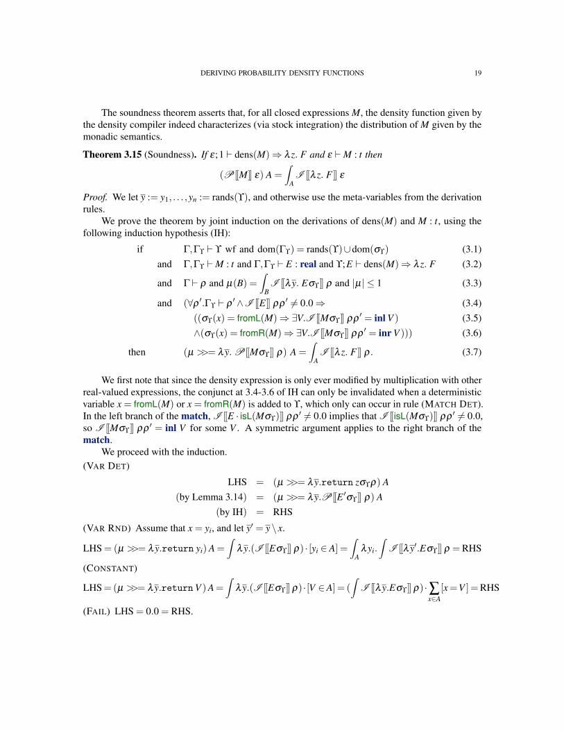
The soundness theorem asserts that, for all closed expressions M, the density function given bythe density compiler indeed characterizes (via stock integration) the distribution of M given by themonadic semantics.
Theorem 3.15 (Soundness). If ε;1 ` dens(M)⇒ λ z. F and ε `M : t then
(P[[M]] ε) A =∫
AI [[λ z. F ]] ε
Proof. We let y := y1, . . . ,yn := rands(ϒ), and otherwise use the meta-variables from the derivationrules.
We prove the theorem by joint induction on the derivations of dens(M) and M : t, using thefollowing induction hypothesis (IH):
if Γ,Γϒ ` ϒ wf and dom(Γϒ) = rands(ϒ)∪dom(σϒ) (3.1)and Γ,Γϒ `M : t and Γ,Γϒ ` E : real and ϒ;E ` dens(M)⇒ λ z. F (3.2)
and Γ ` ρ and µ(B) =∫
BI [[λy. Eσϒ]] ρ and |µ| ≤ 1 (3.3)
and (∀ρ ′.Γϒ ` ρ′∧I [[E]] ρρ
′ 6= 0.0⇒ (3.4)((σϒ(x) = fromL(M)⇒∃V.I [[Mσϒ]] ρρ
′ = inl V ) (3.5)∧(σϒ(x) = fromR(M)⇒∃V.I [[Mσϒ]] ρρ
′ = inr V ))) (3.6)
then (µ >>= λy. P[[Mσϒ]] ρ) A =∫
AI [[λ z. F ]] ρ. (3.7)
We first note that since the density expression is only ever modified by multiplication with otherreal-valued expressions, the conjunct at 3.4-3.6 of IH can only be invalidated when a deterministicvariable x = fromL(M) or x = fromR(M) is added to ϒ, which only can occur in rule (MATCH DET).In the left branch of the match, I [[E · isL(Mσϒ)]] ρρ ′ 6= 0.0 implies that I [[isL(Mσϒ)]] ρρ ′ 6= 0.0,so I [[Mσϒ]] ρρ ′ = inl V for some V . A symmetric argument applies to the right branch of thematch.
We proceed with the induction.(VAR DET)
LHS = (µ >>= λy.return zσϒρ) A(by Lemma 3.14) = (µ >>= λy.P[[E ′σϒ]] ρ) A
(by IH) = RHS
(VAR RND) Assume that x = yi, and let y′ = y\ x.
LHS = (µ >>= λy.return yi) A =∫
λy.(I [[Eσϒ]] ρ) · [yi ∈ A] =∫
Aλyi.
∫I [[λy′.Eσϒ]] ρ = RHS
(CONSTANT)
LHS=(µ >>= λy.returnV )A=∫
λy.(I [[Eσϒ]] ρ)·[V ∈A] = (∫
I [[λy.Eσϒ]] ρ)·∑x∈A
[x=V ] =RHS
(FAIL) LHS = 0.0 = RHS.
20 S. BHAT, J. BORGSTROM, A. D. GORDON, AND C. RUSSO
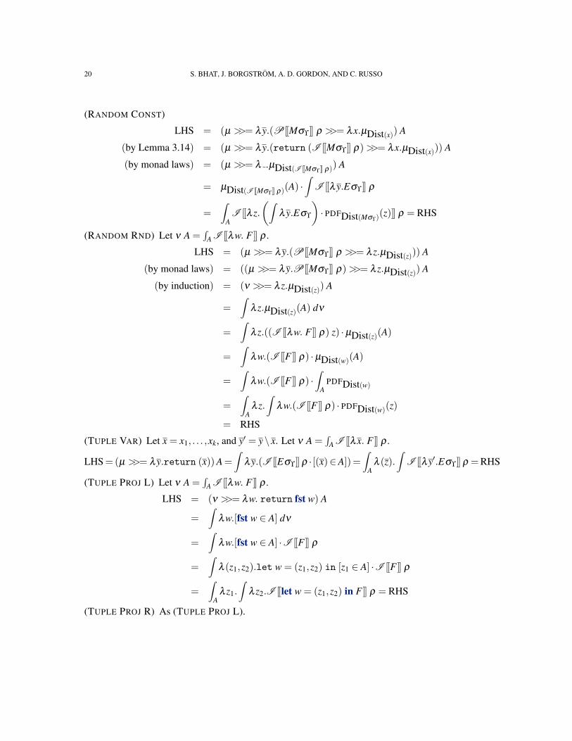
(RANDOM CONST)
LHS = (µ >>= λy.(P[[Mσϒ]] ρ >>= λx.µDist(x)) A
(by Lemma 3.14) = (µ >>= λy.(return (I [[Mσϒ]] ρ)>>= λx.µDist(x))) A
(by monad laws) = (µ >>= λ .µDist(I [[Mσϒ]] ρ)) A
= µDist(I [[Mσϒ]] ρ)(A) ·∫
I [[λy.Eσϒ]] ρ
=∫
AI [[λ z.
(∫λy.Eσϒ
)· PDFDist(Mσϒ)
(z)]] ρ = RHS
(RANDOM RND) Let ν A =∫
A I [[λw. F ]] ρ .
LHS = (µ >>= λy.(P[[Mσϒ]] ρ >>= λ z.µDist(z))) A
(by monad laws) = ((µ >>= λy.P[[Mσϒ]] ρ)>>= λ z.µDist(z)) A
(by induction) = (ν >>= λ z.µDist(z)) A
=∫
λ z.µDist(z)(A) dν
=∫
λ z.((I [[λw. F ]] ρ) z) ·µDist(z)(A)
=∫
λw.(I [[F ]] ρ) ·µDist(w)(A)
=∫
λw.(I [[F ]] ρ) ·∫
APDFDist(w)
=∫
Aλ z.
∫λw.(I [[F ]] ρ) · PDFDist(w)(z)
= RHS
(TUPLE VAR) Let x = x1, . . . ,xk, and y′ = y\ x. Let ν A =∫
A I [[λx. F ]] ρ .
LHS=(µ >>= λy.return (x))A=∫
λy.(I [[Eσϒ]] ρ ·[(x)∈A])=∫
Aλ (z).
∫I [[λy′.Eσϒ]] ρ =RHS
(TUPLE PROJ L) Let ν A =∫
A I [[λw. F ]] ρ .
LHS = (ν >>= λw. return fst w) A
=∫
λw.[fst w ∈ A] dν
=∫
λw.[fst w ∈ A] ·I [[F ]] ρ
=∫
λ (z1,z2).let w = (z1,z2) in [z1 ∈ A] ·I [[F ]] ρ
=∫
Aλ z1.
∫λ z2.I [[let w = (z1,z2) in F ]] ρ = RHS
(TUPLE PROJ R) As (TUPLE PROJ L).
DERIVING PROBABILITY DENSITY FUNCTIONS 21
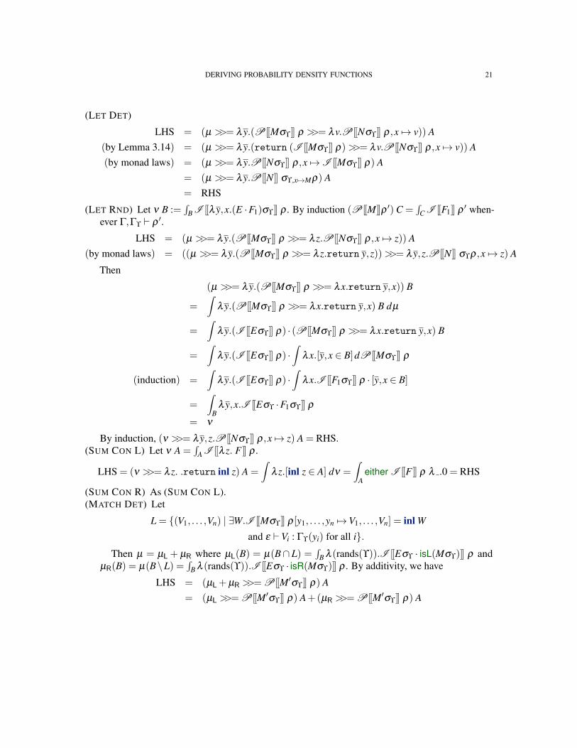
(LET DET)
LHS = (µ >>= λy.(P[[Mσϒ]] ρ >>= λv.P[[Nσϒ]] ρ,x 7→ v)) A(by Lemma 3.14) = (µ >>= λy.(return (I [[Mσϒ]] ρ)>>= λv.P[[Nσϒ]] ρ,x 7→ v)) A(by monad laws) = (µ >>= λy.P[[Nσϒ]] ρ,x 7→I [[Mσϒ]] ρ) A
= (µ >>= λy.P[[N]] σϒ,x 7→Mρ) A= RHS
(LET RND) Let ν B :=∫
B I [[λy,x.(E ·F1)σϒ]] ρ . By induction (P[[M]]ρ ′) C =∫
C I [[F1]] ρ ′ when-ever Γ,Γϒ ` ρ ′.
LHS = (µ >>= λy.(P[[Mσϒ]] ρ >>= λ z.P[[Nσϒ]] ρ,x 7→ z)) A(by monad laws) = ((µ >>= λy.(P[[Mσϒ]] ρ >>= λ z.return y,z))>>= λy,z.P[[N]] σϒρ,x 7→ z) A
Then
(µ >>= λy.(P[[Mσϒ]] ρ >>= λx.return y,x)) B
=∫
λy.(P[[Mσϒ]] ρ >>= λx.return y,x) B dµ
=∫
λy.(I [[Eσϒ]] ρ) · (P[[Mσϒ]] ρ >>= λx.return y,x) B
=∫
λy.(I [[Eσϒ]] ρ) ·∫
λx.[y,x ∈ B]dP[[Mσϒ]] ρ
(induction) =∫
λy.(I [[Eσϒ]] ρ) ·∫
λx.I [[F1σϒ]] ρ · [y,x ∈ B]
=∫
Bλy,x.I [[Eσϒ ·F1σϒ]] ρ
= ν
By induction, (ν >>= λy,z.P[[Nσϒ]] ρ,x 7→ z) A = RHS.(SUM CON L) Let ν A =
∫A I [[λ z. F ]] ρ .
LHS = (ν >>= λ z. .return inl z) A =∫
λ z.[inl z ∈ A] dν =∫
Aeither I [[F ]] ρ λ .0 = RHS
(SUM CON R) As (SUM CON L).(MATCH DET) Let
L = (V1, . . . ,Vn) | ∃W.I [[Mσϒ]] ρ[y1, . . . ,yn 7→V1, . . . ,Vn] = inl W
and ε `Vi : Γϒ(yi) for all i.Then µ = µL + µR where µL(B) = µ(B∩ L) =
∫B λ (rands(ϒ)).I [[Eσϒ · isL(Mσϒ)]] ρ and
µR(B) = µ(B\L) =∫
B λ (rands(ϒ)).I [[Eσϒ · isR(Mσϒ)]] ρ . By additivity, we have
LHS = (µL+µR >>= P[[M′σϒ]] ρ) A= (µL >>= P[[M′σϒ]] ρ) A+(µR >>= P[[M′σϒ]] ρ) A
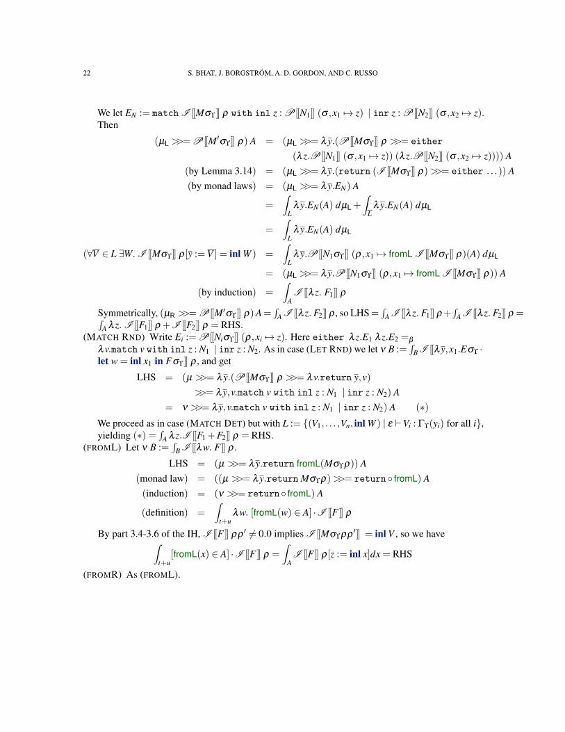
22 S. BHAT, J. BORGSTROM, A. D. GORDON, AND C. RUSSO
We let EN := match I [[Mσϒ]] ρ with inl z : P[[N1]] (σ ,x1 7→ z) | inr z : P[[N2]] (σ ,x2 7→ z).Then
(µL >>= P[[M′σϒ]] ρ) A = (µL >>= λy.(P[[Mσϒ]] ρ >>= either
(λ z.P[[N1]] (σ ,x1 7→ z)) (λ z.P[[N2]] (σ ,x2 7→ z)))) A(by Lemma 3.14) = (µL >>= λy.(return (I [[Mσϒ]] ρ)>>= either . . .)) A(by monad laws) = (µL >>= λy.EN) A
=∫
Lλy.EN(A) dµL+
∫L
λy.EN(A) dµL
=∫
Lλy.EN(A) dµL
(∀V ∈ L ∃W. I [[Mσϒ]] ρ[y :=V ] = inl W ) =∫
Lλy.P[[N1σϒ]] (ρ,x1 7→ fromL I [[Mσϒ]] ρ)(A) dµL
= (µL >>= λy.P[[N1σϒ]] (ρ,x1 7→ fromL I [[Mσϒ]] ρ)) A
(by induction) =∫
AI [[λ z. F1]] ρ
Symmetrically, (µR >>= P[[M′σϒ]] ρ)A=∫
A I [[λ z. F2]] ρ , so LHS=∫
A I [[λ z. F1]] ρ+∫
A I [[λ z. F2]] ρ =∫A λ z. I [[F1]] ρ +I [[F2]] ρ = RHS.
(MATCH RND) Write Ei := P[[Niσϒ]] (ρ,xi 7→ z). Here either λ z.E1 λ z.E2 =β
λv.match v with inl z : N1 | inr z : N2. As in case (LET RND) we let ν B :=∫
B I [[λy,x1.Eσϒ ·let w = inl x1 in Fσϒ]] ρ , and get
LHS = (µ >>= λy.(P[[Mσϒ]] ρ >>= λv.return y,v)>>= λy,v.match v with inl z : N1 | inr z : N2) A
= ν >>= λy,v.match v with inl z : N1 | inr z : N2) A (∗)We proceed as in case (MATCH DET) but with L := (V1, . . . ,Vn, inl W ) | ε `Vi : Γϒ(yi) for all i,yielding (∗) =
∫A λ z.I [[F1 +F2]] ρ = RHS.
(FROML) Let ν B :=∫
B I [[λw. F ]] ρ .
LHS = (µ >>= λy.return fromL(Mσϒρ)) A(monad law) = ((µ >>= λy.return Mσϒρ)>>= return fromL) A(induction) = (ν >>= return fromL) A
(definition) =∫
t+uλw. [fromL(w) ∈ A] ·I [[F ]] ρ
By part 3.4-3.6 of the IH, I [[F ]] ρρ ′ 6= 0.0 implies I [[Mσϒρρ ′]] = inl V , so we have∫t+u
[fromL(x) ∈ A] ·I [[F ]] ρ =∫
AI [[F ]] ρ[z := inl x]dx = RHS
(FROMR) As (FROML).
DERIVING PROBABILITY DENSITY FUNCTIONS 23
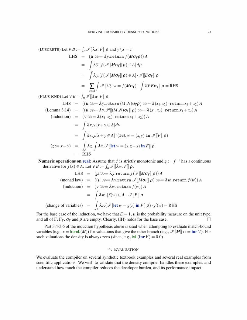
(DISCRETE) Let ν B :=∫
B I [[λx. F ]] ρ and y\ x = z
LHS = (µ >>= λy.return f (Mσϒρ)) A
=∫
λy.[ f (I [[Mσϒ]] ρ) ∈ A]dµ
=∫
λy.[ f (I [[Mσϒ]] ρ) ∈ A] ·I [[Eσϒ]] ρ
= ∑w∈A
∫I [[λ z.[w = f (Mσϒ)] ·
∫λx.Eσϒ]] ρ = RHS
(PLUS RND) Let ν B =∫
B I [[λw. F ]] ρ .
LHS = ((µ >>= λy.return (M,N)σϒρ)>>= λ (x1,x2). return x1 + x2) A(Lemma 3.14) = ((µ >>= λy.P[[(M,N)σϒ]] ρ)>>= λ (x1,x2). return x1 + x2) A
(induction) = (ν >>= λ (x1,x2). return x1 + x2)) A
=∫
λx,y.[x+ y ∈ A]dν
=∫
λx,y.[x+ y ∈ A] · (let w = (x,y) in I [[F ]] ρ)
(z := x+ y) =∫
Aλ z.
∫λx.I [[let w = (x,z− x) in F ]] ρ
= RHS
Numeric operations on real: Assume that f is strictly monotonic and g := f−1 has a continuousderivative for f (x) ∈ A. Let ν B :=
∫B I [[λw. F ]] ρ .
LHS = (µ >>= λy.return f (I [[Mσϒ]] ρ)) A(monad law) = ((µ >>= λy.return I [[Mσϒ]] ρ)>>= λw. return f (w)) A(induction) = (ν >>= λw. return f (w)) A
=∫
λw. [ f (w) ∈ A] ·I [[F ]] ρ
(change of variables) =∫
Aλ z.(I [[let w = g(z) in F ]] ρ) ·g′(w) = RHS
For the base case of the induction, we have that E = 1, µ is the probability measure on the unit type,and all of Γ, Γϒ, σϒ and ρ are empty. Clearly, (IH) holds for the base case.
Part 3.4-3.6 of the induction hypothesis above is used when attempting to evaluate match-boundvariables (e.g., x = fromL(M)) for valuations that give the other branch (e.g., I [[M]] σ = inr V ). Forsuch valuations the density is always zero (since, e.g., isL(inr V ) = 0.0).
4. EVALUATION
We evaluate the compiler on several synthetic textbook examples and several real examples fromscientific applications. We wish to validate that the density compiler handles these examples, andunderstand how much the compiler reduces the developer burden, and its performance impact.
24 S. BHAT, J. BORGSTROM, A. D. GORDON, AND C. RUSSO
4.1. Implementation. Since Fun is a sublanguage of F#, we implement our models as F# programs,and use the quotation mechanism of F# to capture their syntax trees. Running the F# programcorresponds to sampling data from the model. To compute the PDF, the compiler takes the syntaxtree (of F# type Expr) of the model and produces another Expr corresponding to a deterministic F#program as output. We then use run-time code generation to compile the generated Expr to MSILbytecode, which is just-in-time compiled to executable machine code when called, just as for staticallycompiled F# code. Our implementation supports immutable arrays and records, which are bothtranslated using adaptations of the corresponding rules for tuples. For efficiency, the implementationmust avoid introducing redundant computations, translating the use of substitution in the formalrules to more efficient let-bindings that share the values of expressions that would otherwise bere-computed. As is common practice, our implementation and Filzbach (Purves and Lyutsarev, 2012)both work with the logarithm of the density, which avoids products of densities in favor of sumsof log-densities where possible, to avoid numerical underflow. It also performs some simple buteffective peephole optimization to elide canceling applications of Log and Exp and additions of 0.
Code Examples.
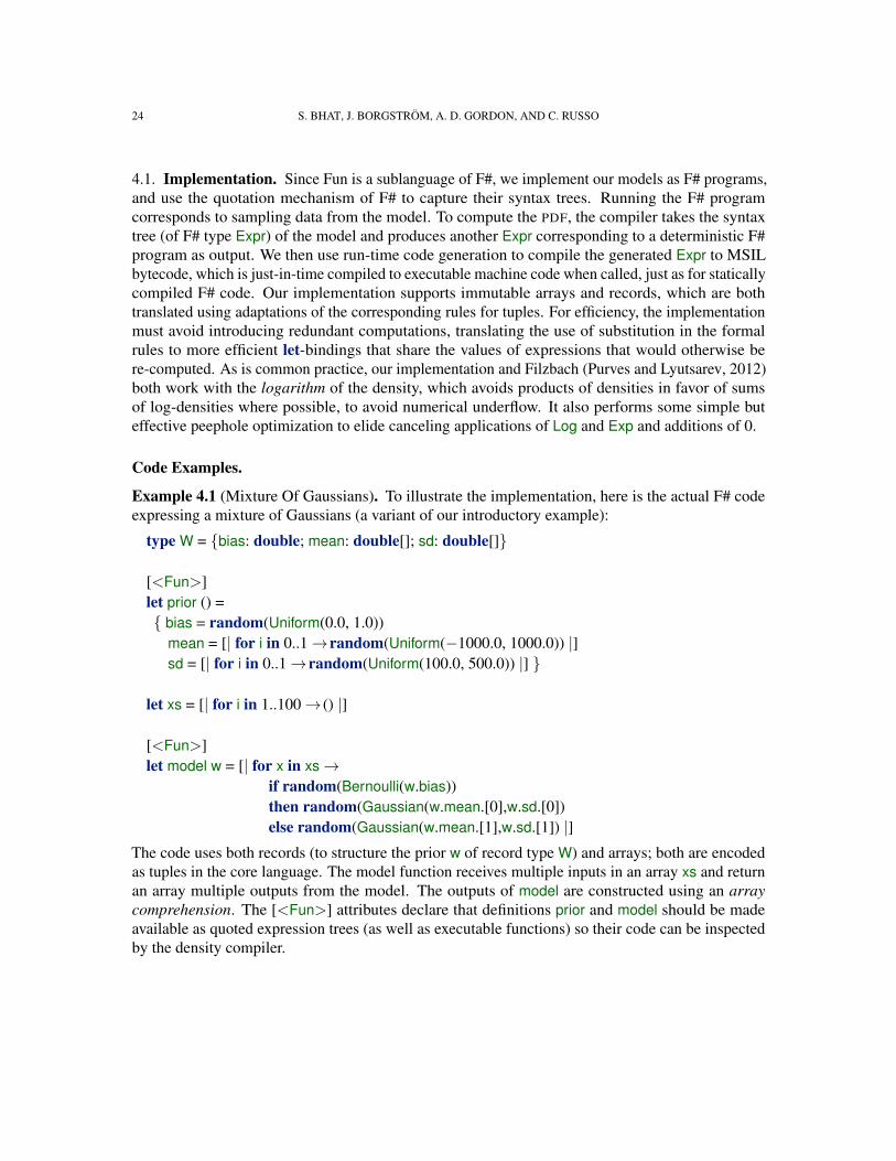
Example 4.1 (Mixture Of Gaussians). To illustrate the implementation, here is the actual F# codeexpressing a mixture of Gaussians (a variant of our introductory example):
type W = bias: double; mean: double[]; sd: double[]
[<Fun>]let prior () = bias = random(Uniform(0.0, 1.0))
mean = [| for i in 0..1→random(Uniform(−1000.0, 1000.0)) |]sd = [| for i in 0..1→random(Uniform(100.0, 500.0)) |]
let xs = [| for i in 1..100→ () |]
[<Fun>]let model w = [| for x in xs→
if random(Bernoulli(w.bias))then random(Gaussian(w.mean.[0],w.sd.[0])else random(Gaussian(w.mean.[1],w.sd.[1]) |]
The code uses both records (to structure the prior w of record type W) and arrays; both are encodedas tuples in the core language. The model function receives multiple inputs in an array xs and returnan array multiple outputs from the model. The outputs of model are constructed using an arraycomprehension. The [<Fun>] attributes declare that definitions prior and model should be madeavailable as quoted expression trees (as well as executable functions) so their code can be inspectedby the density compiler.
DERIVING PROBABILITY DENSITY FUNCTIONS 25
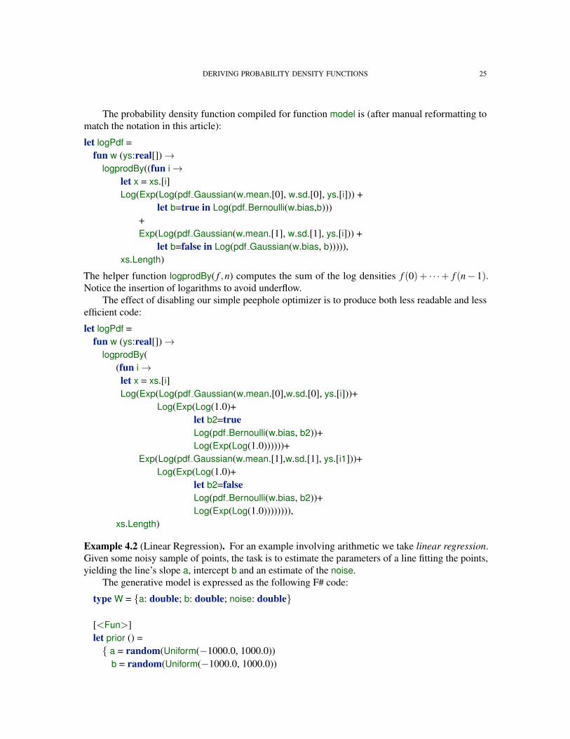
The probability density function compiled for function model is (after manual reformatting tomatch the notation in this article):
let logPdf =fun w (ys:real[])→
logprodBy((fun i→let x = xs.[i]Log(Exp(Log(pdf Gaussian(w.mean.[0], w.sd.[0], ys.[i])) +
let b=true in Log(pdf Bernoulli(w.bias,b)))+Exp(Log(pdf Gaussian(w.mean.[1], w.sd.[1], ys.[i])) +
let b=false in Log(pdf Gaussian(w.bias, b))))),xs.Length)
The helper function logprodBy( f ,n) computes the sum of the log densities f (0)+ · · ·+ f (n− 1).Notice the insertion of logarithms to avoid underflow.
The effect of disabling our simple peephole optimizer is to produce both less readable and lessefficient code:
let logPdf =fun w (ys:real[])→
logprodBy((fun i→let x = xs.[i]Log(Exp(Log(pdf Gaussian(w.mean.[0],w.sd.[0], ys.[i]))+
Log(Exp(Log(1.0)+let b2=trueLog(pdf Bernoulli(w.bias, b2))+Log(Exp(Log(1.0))))))+
Exp(Log(pdf Gaussian(w.mean.[1],w.sd.[1], ys.[i1]))+Log(Exp(Log(1.0)+
let b2=falseLog(pdf Bernoulli(w.bias, b2))+Log(Exp(Log(1.0)))))))),
xs.Length)
Example 4.2 (Linear Regression). For an example involving arithmetic we take linear regression.Given some noisy sample of points, the task is to estimate the parameters of a line fitting the points,yielding the line’s slope a, intercept b and an estimate of the noise.
The generative model is expressed as the following F# code:
type W = a: double; b: double; noise: double
[<Fun>]let prior () = a = random(Uniform(−1000.0, 1000.0))
b = random(Uniform(−1000.0, 1000.0))
26 S. BHAT, J. BORGSTROM, A. D. GORDON, AND C. RUSSO
noise = random(Uniform(0.001, 100.0))
let xs = [| −100.0 .. 100.0 |]
[<Fun>]let model w = [| for x in xs→
let m = w.a ∗ x + w.blet d = w.noiserandom(Gaussian(m, d)) |]
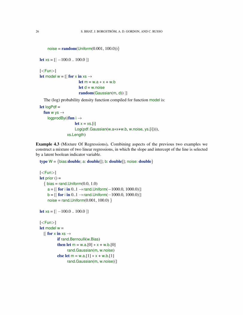
The (log) probability density function compiled for function model is:
let logPdf =fun w ys→
logprodBy((fun i→let x = xs.[i]Log(pdf Gaussian(w.a∗x+w.b, w.noise, ys.[i]))),
xs.Length)
Example 4.3 (Mixture Of Regressions). Combining aspects of the previous two examples weconstruct a mixture of two linear regressions, in which the slope and intercept of the line is selectedby a latent boolean indicator variable.
type W = bias:double; a: double[]; b: double[]; noise: double
[<Fun>]let prior () = bias = rand.Uniform(0.0, 1.0)
a = [| for i in 0..1→ rand.Uniform(−1000.0, 1000.0)|]b = [| for i in 0..1→ rand.Uniform(−1000.0, 1000.0)|]noise = rand.Uniform(0.001, 100.0)
let xs = [| −100.0 .. 100.0 |]
[<Fun>]let model w =
[| for x in xs→if rand.Bernoulli(w.Bias)then let m = w.a.[0] ∗ x + w.b.[0]
rand.Gaussian(m, w.noise)else let m = w.a.[1] ∗ x + w.b.[1]
rand.Gaussian(m, w.noise)|]
DERIVING PROBABILITY DENSITY FUNCTIONS 27
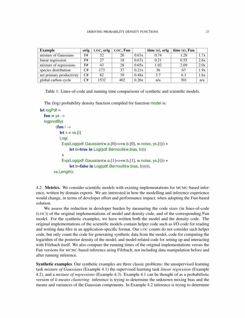
Example orig LOC, orig LOC, Fun time (s), orig time (s), Funmixture of Gaussians F# 32 20 0.63x 0.74 1.28 1.7xlinear regression F# 27 18 0.67x 0.21 0.55 2.6xmixture of regressions F# 43 28 0.65x 1.02 2.09 2.0xspecies distribution C# 173 37 0.21x 36 67 1.9xnet primary productivity C# 82 39 0.48x 3.7 6.1 1.6xglobal carbon cycle C# 1532 402 0.26x n/a 301 n/a
Table 1: Lines-of-code and running time comparisons of synthetic and scientific models.
The (log) probability density function compiled for function model is:
let logPdf =fun w ys→logprodBy(
(fun i→let x = xs.[i]Log(Exp(Log(pdf Gaussian(w.a.[0]∗x+w.b.[0], w.noise, ys.[i])) +
let b=true in Log(pdf Bernoulli(w.bias, b)))+Exp(Log(pdf Gaussian(w.a.[1]∗x+w.b.[1], w.noise, ys.[i])) +
let b=false in Log(pdf Bernoulli(w.bias, b))))),xs.Length);
4.2. Metrics. We consider scientific models with existing implementations for MCMC-based infer-ence, written by domain experts. We are interested in how the modelling and inference experiencewould change, in terms of developer effort and performance impact, when adopting the Fun-basedsolution.
We assess the reduction in developer burden by measuring the code sizes (in lines-of-code(LOC)) of the original implementations of model and density code, and of the corresponding Funmodel. For the synthetic examples, we have written both the model and the density code. Theoriginal implementations of the scientific models contain helper code such as I/O code for readingand writing data files in an application-specific format. Our LOC counts do not consider such helpercode, but only count the code for generating synthetic data from the model, code for computing thelogarithm of the posterior density of the model, and model-related code for setting up and interactingwith Filzbach itself. We also compare the running times of the original implementations versus theFun versions for MCMC-based inference using Filzbach, not including data manipulation before andafter running inference.
Synthetic examples. Our synthetic examples are three classic problems: the unsupervised learningtask mixture of Gaussians (Example 4.1) the supervised learning task linear regression (Example4.2), and a mixture of regressions (Example 4.3). Example 4.1 can be thought of as a probabilisticversion of k-means clustering: inference is trying to determine the unknown mixing bias and themeans and variances of the Gaussian components. In Example 4.2 inference is trying to determine
28 S. BHAT, J. BORGSTROM, A. D. GORDON, AND C. RUSSO
the coefficients of the line. In Example 4.3 inference is trying to determine the coefficients andmixing bias of two lines.
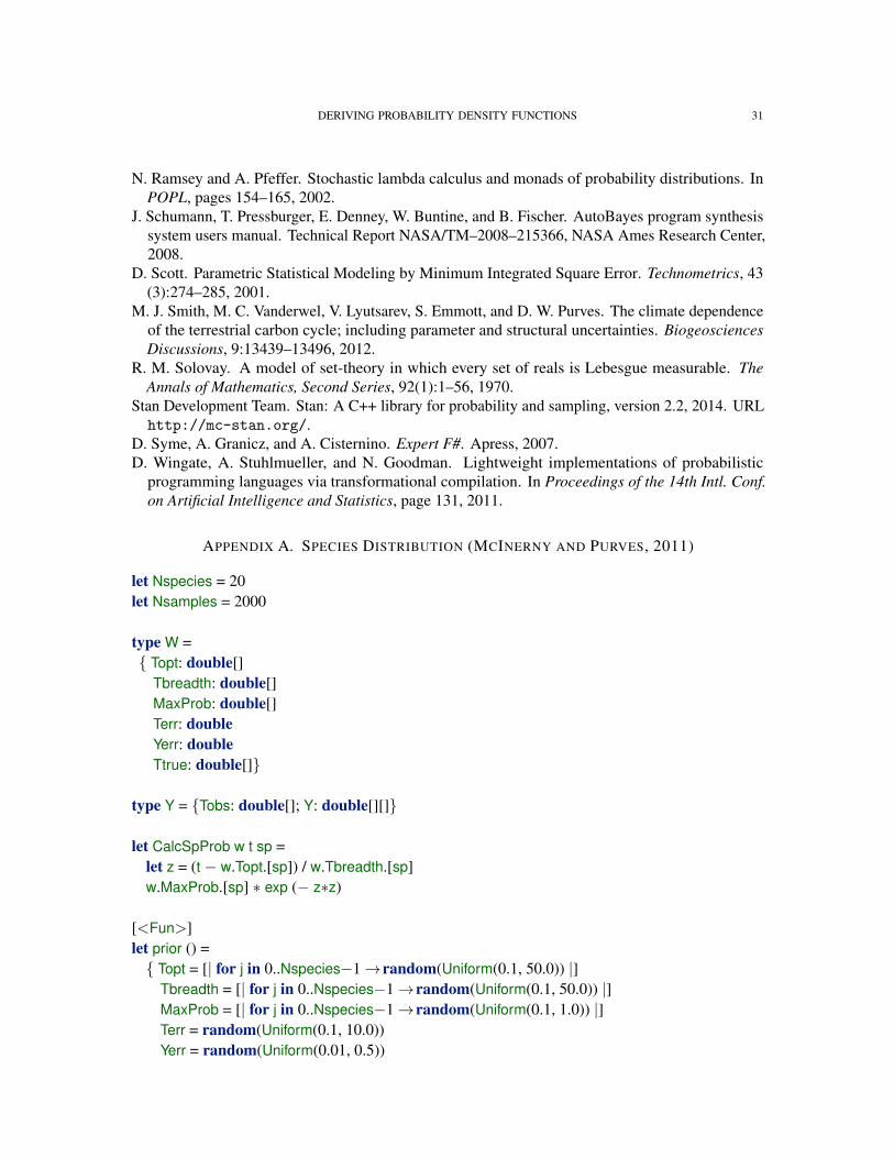
Species distribution (McInerny and Purves, 2011). The species distribution problem is to give theprobability that certain species will be present at a given site, based on climate factors. It is a problemof long-standing interest in ecology and has taken on new relevance in light of the issue of climatechange. The particular model that we consider is designed to mitigate regression dilution arisingfrom uncertainty in the predictor variables, for example, measurement error in temperature data.Inference tries to determine various features of the species and the environment, such as the optimaltemperature preferred by a species, or the true temperature at a site (see code and density function inAppendix A).
Global carbon cycle. (Smith et al., 2012). The dynamics of the Earth’s climate are intertwinedwith the terrestrial carbon cycle, and better carbon models (modelling how carbon in the air getsconverted to biomass) enable better constrained projections about these systems. We consider afully data-constrained terrestrial carbon model, which is composed of various submodels for smallerprocesses such as net primary productivity, the fine root mortality rate, or the fraction of trees that areevergreen versus deciduous. Inference tries to determine the different parameters of these submodels.
Discussion. Table 1 reports the metrics for each example. The LOC numbers show significantreduction in code size, with more significant savings as the size of the model grows. The largermodels (where the Fun versions are ≈ 25% of the size of the original) are more indicative of thesavings in developer and maintenance effort because Filzbach interaction code, which is roughlythe same in all models, takes up a larger fraction of the smaller models. We find the running timesencouraging: we have made little attempt to optimize the generated code, and preliminary testingindicates that much of the performance slow-down is due to constant factors.
The global carbon cycle model is composed of submodels, each with their own dataset. Un-fortunately, it is unclear from the original source code how this composition translates to a run ofinference, making it difficult to know what constitutes a fair comparison. Thus, we do not report arunning time for the full model. However, we can measure the running time of individual submodels,such as net primary productivity, where the data and control flow are simpler.
5. RELATED WORK
We have presented the first algorithm for deriving density functions from generative processes, thatis both proved correct and implemented. An abridged version of this paper appears as Bhat et al.(2013). The correctness proof (for a version of the source language without pure let and generalmatch) was recently mechanized in Isabelle by Eberl et al. (2015).
This paper builds on work by Bhat et al. (2012) who develop a theoretical framework forcomputing PDFs, but describe no implementation nor correctness proof. The density compiler ofSection 3 has a simpler presentation, with two judgments compared to five, and has rules for purelets and operations on integers. Our paper also uses a richer language (Fun), which adds fail, matchand general if (and for performance reasons, pure let).
Gordon et al. (2013) describe a naive density calculation routine for Fun without random lets;this sublanguage does not cover many useful classes of models such as hierarchical and mixturemodels.
The BUGS system computes densities from declaratively specified models to perform Gibbssampling (Gilks et al., 1994). However, the models are not compositional as in this work, and only the
DERIVING PROBABILITY DENSITY FUNCTIONS 29
joint density over all variables is possible. The AutoBayes system also computes densities for derivingmaximum likelihood and Bayesian estimators for a significant class of statistical models (Schumannet al., 2008). It is not formally specified and does not appear to be compositional. Neither systemaddresses the non-existence of PDFs, presumably restricting expressivity in order to avoid the issue.
Stan (Stan Development Team, 2014) is a probabilistic programming language that supportsvarious forms of MCMC. The Stan language is a derivative of BUGS, and is compiled to efficientC++ sampling code, in part based on automatically derived density functions. For models with latentvariables, including mixture models such as mixture of Gaussians, and for models that performnon-linear computations on random values, Stan’s users are required to manually manipulate thelog probability density function, using a primitive operation increment log prob. Stan employsautomatic differentiation (Griewank and Walther, 2008) of log posteriors in order to apply gradient-based Hamiltonian MCMC algorithms. This relieves the user from coding error-prone derivatives.
Inference for the Church language also uses MCMC, but works with distributions over runs of aprogram instead of over its return value (Wingate et al., 2011), circumventing the need for a PDF.
There are many other systems for probabilistic programming, some of which provide a way tocompute density functions or an analogous object; however, they sacrifice some other feature to doso. Several languages only provide support for finite, discrete distributions, but provide access to theprobability mass function (Ramsey and Pfeffer, 2002; Kiselyov and Shan, 2009). Like BUGS andStan, systems like the Hierarchical Bayes Compiler (Daume III, 2007) are not formally defined andrequire models to be specified in a monolithic way, whereas large models in Fun can be composed ofsmaller models. Probabilistic logic languages like Markov Logic (Domingos et al., 2008) do not havegenerative semantics but instead have semantics in undirected graphical models which are equippedwith potential functions that are analogous to density functions. The language is constructed in a waythat guarantees the existence of a potential function, but which eliminates the possibility to expressmodels that require pure let, such as the global carbon cycle model.
6. CONCLUSIONS AND FUTURE WORK
We have described a compiler for automatically computing probability density functions for programsfrom a rich Bayesian probabilistic programming language, proven the algorithm correct, and shownits applicability to real-world scientific models.
The inclusion of fail in the language appears useful for scientific models, giving a simplefacility to exclude branches that are scientifically impossible from consideration. However, moreinvestigation is needed to settle this claim.
A drawback of the compiler is that terms of composite type are required either to have a PDF orto be pure, ruling out terms such as (0.0, random(Uniform)). One possibility for future work wouldbe to refine the types of expressions with determinacy information, and make use of this additionalinformation to admit more joint distributions (cf. (TUPLE VAR)).
ACKNOWLEDGMENTS
We thank Manuel Eberl and Tobias Nipkow for helpful comments, in particular on the semantics ofthe integration operator.
30 S. BHAT, J. BORGSTROM, A. D. GORDON, AND C. RUSSO
REFERENCES
A. Ben-Israel. The change of variables formula using matrix volume. SIAM Journal of MatrixAnalysis, 21:300–312, 1999.
S. Bhat, A. Agarwal, R. W. Vuduc, and A. G. Gray. A type theory for probability density functions.In J. Field and M. Hicks, editors, POPL, pages 545–556. ACM, 2012.
S. Bhat, J. Borgstrom, A. D. Gordon, and C. Russo. Deriving probability density functions fromprobabilistic functional programs. In Tools and Algorithms for the Construction and Analysis ofSystems, 19th International Conference: TACAS 2013, number 7795 in LNCS, pages 508–522.Springer, 2013.
C. M. Bishop. Pattern Recognition and Machine Learning. Springer Science + Business Media,LLC, New York, NY, USA, 2006.
J. Borgstrom, A. D. Gordon, M. Greenberg, J. Margetson, and J. Van Gael. Measure trans-former semantics for Bayesian machine learning. In European Symposium on Programming(ESOP’11), volume 6602 of LNCS, pages 77–96. Springer, 2011. Download available athttps://www.microsoft.com/en-us/research/project/infer-net-fun/.
H. Daume III. HBC: Hierarchical Bayes Compiler, 2007. URL http://hal3.name/HBC.P. Domingos, S. Kok, D. Lowd, H. Poon, M. Richardson, and P. Singla. Markov logic. In L. De Raedt,
P. Frasconi, K. Kersting, and S. Muggleton, editors, Probabilistic inductive logic programming,pages 92–117. Springer-Verlag, Berlin, Heidelberg, 2008.
M. Eberl, J. Holzl, and T. Nipkow. A verified compiler for probability density functions. In J. Vitek,editor, 24th European Symposium on Programming: ESOP 2015, number 9032 in LNCS, pages80–104. Springer, 2015.
W. R. Gilks, A. Thomas, and D. J. Spiegelhalter. A language and program for complex Bayesianmodelling. The Statistician, 43:169–178, 1994.
M. Giry. A categorical approach to probability theory. In B. Banaschewski, editor, CategoricalAspects of Topology and Analysis, volume 915 of Lecture Notes in Mathematics, pages 68–85.Springer Berlin / Heidelberg, 1982.
N. Goodman, V. K. Mansinghka, D. M. Roy, K. Bonawitz, and J. B. Tenenbaum. Church: a languagefor generative models. In Uncertainty in Artificial Intelligence (UAI’08), pages 220–229. AUAIPress, 2008.
A. D. Gordon, M. Aizatulin, J. Borgstrom, G. Claret, T. Graepel, A. Nori, S. Rajamani, and C. Russo.A model-learner pattern for Bayesian reasoning. In POPL, 2013.
A. Griewank and A. Walther. Evaluating Derivatives: Principles and Techniques of AlgorithmicDifferentiation. SIAM, 2nd edition, 2008.
O. Kiselyov and C. Shan. Embedded probabilistic programming. In Domain-Specific Languages,pages 360–384, 2009.
G. McInerny and D. Purves. Fine-scale environmental variation in species distribution modelling:regression dilution, latent variables and neighbourly advice. Methods in Ecology and Evolution, 2(3):248–257, 2011.
R. M. Neal. Probabilistic inference using Markov chain Monte Carlo methods. Technical ReportCRG-TR-93-1, Dept. of Computer Science, University of Toronto, September 1993.
P. Panangaden. The category of Markov kernels. Electronic Notes in Theoretical Computer Science,22:171–187, 1999.
D. Purves and V. Lyutsarev. Filzbach User Guide, 2012. Available athttps://www.microsoft.com/en-us/download/details.aspx?id=52465.
DERIVING PROBABILITY DENSITY FUNCTIONS 31
N. Ramsey and A. Pfeffer. Stochastic lambda calculus and monads of probability distributions. InPOPL, pages 154–165, 2002.
J. Schumann, T. Pressburger, E. Denney, W. Buntine, and B. Fischer. AutoBayes program synthesissystem users manual. Technical Report NASA/TM–2008–215366, NASA Ames Research Center,2008.
D. Scott. Parametric Statistical Modeling by Minimum Integrated Square Error. Technometrics, 43(3):274–285, 2001.
M. J. Smith, M. C. Vanderwel, V. Lyutsarev, S. Emmott, and D. W. Purves. The climate dependenceof the terrestrial carbon cycle; including parameter and structural uncertainties. BiogeosciencesDiscussions, 9:13439–13496, 2012.
R. M. Solovay. A model of set-theory in which every set of reals is Lebesgue measurable. TheAnnals of Mathematics, Second Series, 92(1):1–56, 1970.
Stan Development Team. Stan: A C++ library for probability and sampling, version 2.2, 2014. URLhttp://mc-stan.org/.
D. Syme, A. Granicz, and A. Cisternino. Expert F#. Apress, 2007.D. Wingate, A. Stuhlmueller, and N. Goodman. Lightweight implementations of probabilistic
programming languages via transformational compilation. In Proceedings of the 14th Intl. Conf.on Artificial Intelligence and Statistics, page 131, 2011.
APPENDIX A. SPECIES DISTRIBUTION (MCINERNY AND PURVES, 2011)
let Nspecies = 20let Nsamples = 2000
type W = Topt: double[]
Tbreadth: double[]MaxProb: double[]Terr: doubleYerr: doubleTtrue: double[]
type Y = Tobs: double[]; Y: double[][]
let CalcSpProb w t sp =let z = (t − w.Topt.[sp]) / w.Tbreadth.[sp]w.MaxProb.[sp] ∗ exp (− z∗z)
[<Fun>]let prior () = Topt = [| for j in 0..Nspecies−1→random(Uniform(0.1, 50.0)) |]
Tbreadth = [| for j in 0..Nspecies−1→random(Uniform(0.1, 50.0)) |]MaxProb = [| for j in 0..Nspecies−1→random(Uniform(0.1, 1.0)) |]Terr = random(Uniform(0.1, 10.0))Yerr = random(Uniform(0.01, 0.5))
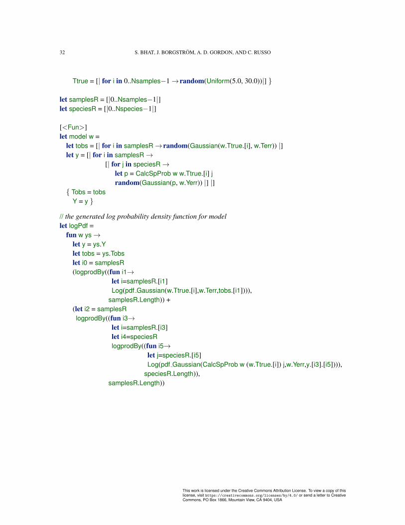
32 S. BHAT, J. BORGSTROM, A. D. GORDON, AND C. RUSSO
Ttrue = [| for i in 0..Nsamples−1→random(Uniform(5.0, 30.0))|]
let samplesR = [|0..Nsamples−1|]let speciesR = [|0..Nspecies−1|]
[<Fun>]let model w =
let tobs = [| for i in samplesR→random(Gaussian(w.Ttrue.[i], w.Terr)) |]let y = [| for i in samplesR→
[| for j in speciesR→let p = CalcSpProb w w.Ttrue.[i] jrandom(Gaussian(p, w.Yerr)) |] |]
Tobs = tobsY = y
// the generated log probability density function for modellet logPdf =
fun w ys→let y = ys.Ylet tobs = ys.Tobslet i0 = samplesR(logprodBy((fun i1→
let i=samplesR.[i1]Log(pdf Gaussian(w.Ttrue.[i],w.Terr,tobs.[i1]))),
samplesR.Length)) +(let i2 = samplesRlogprodBy((fun i3→
let i=samplesR.[i3]let i4=speciesRlogprodBy((fun i5→
let j=speciesR.[i5]Log(pdf Gaussian(CalcSpProb w (w.Ttrue.[i]) j,w.Yerr,y.[i3].[i5]))),
speciesR.Length)),samplesR.Length))
This work is licensed under the Creative Commons Attribution License. To view a copy of thislicense, visit https://creativecommons.org/licenses/by/4.0/ or send a letter to CreativeCommons, PO Box 1866, Mountain View, CA 9404, USA