on optimization algorithms for the reservoir oil well ... · on optimization algorithms for the...

On Optimization Algorithms for the Reservoir Oil WellPlacement Problem

W. Bangerth ([email protected])Center for Subsurface Modeling, Institute for Computational Engineering and Sciences; andInstitute for Geophysics, The University of Texas at Austin, Austin, TX 78712

H. Klie ([email protected]) and M. F. Wheeler([email protected])Center for Subsurface Modeling, Institute for Computational Engineering and Sciences, TheUniversity of Texas at Austin, Austin, TX 78712

P. L. Stoffa ([email protected]) and M. K. Sen([email protected])Institute for Geophysics, John A. and Katherine G. Jackson School of Geosciences, TheUniversity of Texas at Austin, Austin, TX 78712

Abstract. Determining optimal locations and operation parameters for wells in oil and gasreservoirs has a potentially high economic impact. Finding these optima depends on a complexcombination of geological, petrophysical, flow regimen, and economical parameters that arehard to grasp intuitively. On the other hand, automatic approaches have in the past been ham-pered by the overwhelming computational cost of running thousands of potential cases usingreservoir simulator, given that each of these runs can take on the order of hours. Therefore,the key issue to such automatic optimization is the development of algorithms that find goodsolutions with a minimum number of function evaluations. In this work, we compare andanalyze the efficiency, effectiveness, and reliability of several optimization algorithms for thewell placement problem. In particular, we consider the Simultaneous Perturbation StochasticApproximation (SPSA), Finite Difference Gradient (FDG), and Very Fast Simulated Anneal-ing (VFSA) algorithms. None of these algorithms guarantees to find the optimal solution, butwe show that both SPSA and VFSA are very efficient in finding nearly optimal solutions witha high probability. We illustrate this with a set of numerical experiments based on real data forsingle and multiple well placement problems.

Keywords: well placement, reservoir optimization, reservoir simulation, stochastic optimiza-tion, SPSA, simulated annealing, VFSA

1. Introduction

The placement, operation scheduling, and optimization of one or many wellsduring a given period of the reservoir production life has been a focus of atten-tion of oil production companies and environmental agencies in the last years.In the petroleum engineering scenario, the basic premise of this problem is toachieve the maximum revenue from oil and gas while minimizing operatingcosts, subject to different geological and economical constraints. This is achallenging problem since it requires many large scale reservoir simulations

c�

2004 Kluwer Academic Publishers. Printed in the Netherlands.

compSPSA.tex; 21/10/2004; 10:45; p.1

2 W. Bangerth et al.

and needs to take into account uncertainty in the reservoir description. Evenif a large number of scenarios is considered and analyzedby experienced en-gineers, the procedure is in most cases inefficient and delivers solutions farfrom the optimal one. Consequently, important economical losses may result.

Optimization algorithms provide a systematic way to explore a broaderset of scenarios and aim at finding very good or optimal ones for some givenconditions. In conjunction with specialists, these algorithms provide a pow-erful mean to reduce the risk in decision-making. Nevertheless, the majordrawback in using optimization algorithms is the cost of repeatedly evaluatingdifferent exploitation scenarios by numerical simulation based on a complexset of coupled nonlinear partial differential equations on hundreds of thou-sands to millions of gridblocks. Therefore, the major challenge in relying onautomatic optimization algorithms is finding methods that are efficient androbust in delivering a set of nearly optimal solutions.

In the past, a number of algorithms has been devised and analyzed for op-timization and inverse problems in reservoir simulation, see e.g. [26, 33, 46].These problems basically fall within four categories: (1) history matching; (2)well location; (3) production scheduling; and, (4) surface facility design. Inthe particular case of the well placement problem, the use of optimization al-gorithms began to be reported about 10 years ago, see e.g. [4, 35]. Since then,increasingly complicated cases have been reported in the literature, mainly inthe directions of complex well models (type, number, orientation), character-istics of the reservoir under study, and the numerical approaches employed forits simulation [5, 14, 13, 29, 43, 44]. From an optimization standpoint, mostalgorithms employed so far are either stochastic or heuristic approaches; inparticular, this includes simulated annealing (SA) [4] and genetic algorithms(GA) [14, 44]. Some of them have also been combined with deterministic ap-proaches to provide a fast convergence close to the solution; for instance, GAwith polytope and tabu search [5] and GA with neural networks [14, 7]. In allcases, the authors point out that all these algorithms are still computationallydemanding for large scale applications.

In this work, we introduce the simultaneous perturbation stochastic ap-proximation (SPSA) method to the well placement problem, and compare itsproperties with other, better known algorithms. The SPSA algorithm can beseen as a stochastic version of the steepest descent method where a stochasticvector replaces the gradient vector computed using point-wise finite differ-ence approximations in each of the directions associated with the decisionvariables. This generates a highly efficient method since the number of func-tion evaluations per step does not depend on the dimension of the searchspace. Despite the fact that the algorithm has a local search character in itssimplest form, the stochastic components of the algorithm are capable of de-livering nearly optimal solutions in relatively few steps. Hence, we show thatthis approach is more efficient than other traditional algorithms employed for

compSPSA.tex; 21/10/2004; 10:45; p.2

On optimization algorithms for the well placement problem 3

the well placement problem. Moreover, the capability of the SPSA algorithmto adapt easily from local search to global search makes it attractive for futurehybrid implementations.

This paper is organized as follows: Section 2 reviews the components thatare used for the solution of the well placement problem: (1) the reservoirmodel and the parallel reservoir simulator used for forward modelling; (2) theeconomic revenue function to optimize; and, (3) the optimization algorithmsconsidered under this comparative study. Section 3 shows an exhaustive andcomparative treatment of these algorithms based on the placement of onewell. Section 4 extends the previous numerical analysis to the placement ofmultiple wells. Section 5 summarizes the results of the present work anddiscusses possible directions of further research.

2. Problem description and approaches

In this study, we pose the following optimization question: at which positionshould a (set of) new injection/production wells be placed to maximize theeconomic revenue of production in the future? We first detail the descriptionof the reservoir simulator that allows the evaluation of this economic revenueobjective function. We then proceed to describe the objective function andits dependence on coefficients such as costs for injection and production. Weend the section by describing the algorithms that were considered for solvingthis optimization problem.

2.1. DESCRIPTION AND SOLUTION OF THE OIL RESERVOIR MODEL

For the purpose of this paper, we restrict our analysis to reservoirs that can bedescribed by a two-phase, oil-water model. This model can be formulated asthe following set of partial differential equations for the conservation of massof each phase �� (oil and water):

� �� (1)

Here,�

is the porosity of the porous medium,� �

is the concentrationof the phase � , and � � represents the source/sink term (production/injectionwells). The fluxes � � are defined using Darcy’s law [15] which, with gravityignored, reads as � � ��!#" �%$'&(� �*) � , where " � denotes the density of thephase,

$the permeability tensor,

&+�the mobility of the phase, and ) � the

pressure of phase � . Additional equations specifying volume, capillary, andstate constraints are added, and boundary and initial conditions complementthe system, see [2, 15]. Finally,

� � �-, � " � with , � denoting saturation of

compSPSA.tex; 21/10/2004; 10:45; p.3


a phase. The resulting system for this formulation is � " � , �� ! �� " � $'& � � ) �� (2)

In this paper we consider wells that either produce (a mixture of) oil andwater, or at which water is injected. At an injection well, the source term � �is nonnegative (we use the notation � �� to make this explicit). At aproduction well, both �� and � � may be non-positive and we denote this by�� ! � � . In practice, both injection and production rates are subject tocontrol, and thus to optimization; however, in this paper we assume that ratesare indirectly defined through the specification of the bottom hole pressure(BHP). These rates are used for evaluating the objective function and are notdecision parameters in our optimization problem.

This model is discretized in space using the expanded mixed finite elementmethod which, in the case considered in this paper, is numerically equivalentto the cell-centered finite difference approach [1, 36]. In time, we use a fullyimplicit formulation solved at every time step with a Newton-Krylov methodpreconditioned with algebraic multigrid.

The discrete model is solved with the IPARS (Integrated Parallel Accu-rate Reservoir Simulator) software developed at the Center for SubsurfaceModelling at The University of Texas at Austin (see, e.g., [25, 31, 34, 40,42]). IPARS is a parallel reservoir simulation framework that allows for dif-ferent algorithms or formulations (IMPES, fully implicit), different physics(compositional, gas-oil-water, air-water and one-phase flow) and differentdiscretizations in different parts of the domain by means of the multiblockapproach [24, 23, 32, 41, 45]. It offers sophisticated simulation componentsthat encapsulate complex mathematical models of the physical interactionin the subsurface such as geomechanics and chemical processes, and whichexecute on parallel and distributed systems. Solvers employ state-of-the-arttechniques for nonlinear and linear problems including Newton-Krylov meth-ods enhanced with multigrid, two-stage and physics-based preconditioners[20, 21]. It can also handle an arbitrary number of wells each with one ormore completion intervals.

2.2. ECONOMIC MODEL

In general, the economic value of production is a function of the time ofproduction and of injection and production rates in the reservoir. It takes intoaccount costs such as well drilling, oil prices, costs of injection, extraction,and disposal of water and of the hydrocarbons, as well as associated operatingcosts. We assume here that operation and drilling costs are independent of thewell locations and therefore a constant part of our objective function that canbe omitted for the purpose of optimization.

compSPSA.tex; 21/10/2004; 10:45; p.4


We then define our objective function by summing up, over the time hori-zon

�� , the revenues from produced oil over all production wells, andsubtracting the costs of disposing produced water and the cost of injectingwater. The result is the net present value (NPV) function�� ! � �

�� ! #" � � �� ! " �%$ �'& �#� � �� (*)! �&,+�-.� �� " �/$ &,+�- � �� 10 �2 �43 � �65�7 � � (3)

where � �� and � �� are production rates for oil and water, respectively, and � ��are water injection rates, each in barrel per day. The coefficients " � , " �%$ �'& �8�and " �/$ &,+�- are the prices of oil and the costs of disposing and injecting water,in units of dollars per barrel each. The term 3 represents the interest rate perday, and the exponential factor takes into account that the drilling costs haveto be paid up front and have to be paid off with interest. The function

�9� � �is the negative total NPV, as our algorithms will be searching for a minimum;this then amounts to maximizing the (positive) revenue.

If no confusion is possible, we drop the subscript from�:�

when we com-pare function evaluations for the same time horizon � but different welllocations

. Note that

� � �depends on the locations

of the wells in two

ways. First, the injection rates of wells, and thus their associated costs, dependon their location if the bottom hole pressure (BHP) is prescribed. Secondly,the production rates of the wells as well as their water-oil ratio depend onwhere water is injected and where producers are located.

We remark that in practice, realistic objective functions would also includeother factors that would render it more complex (see, e.g., [6, 9]). The generalform would be the same, however.

2.3. THE OPTIMIZATION PROBLEM

With the model and objective function described above, the optimizationproblem is stated as follows: find optimal well locations

%;such that ; �=<?>.@BADCFE�?G?H � � � � (4)

subject to the flow variables used in� � �

satisfying model (1)–(2). The pa-rameter space for optimization ) is the set of possible well locations. Sincewe discretize the model shown above for solution on a computer, possiblewell locations are only a discrete set of points on an integer lattice, ratherthan a continuum, and optimization algorithms have to take this into account.We fix the bottom hole pressure (BHP) operating conditions at all wells.

compSPSA.tex; 21/10/2004; 10:45; p.5


However, in general the BHP and possibly other parameters could vary andbecome an element of ) as well.

In the rest of the section, we briefly describe all the optimization algo-rithms that we compare for their performance on the problem outlined above.The implementation of these algorithms uses a Grid enabled software frame-work previously described in [3, 19, 30].

2.3.1. An integer SPSA algorithmThe first optimization algorithm we consider is an integer version of the Si-multaneous Perturbation Stochastic Approximation (SPSA) method. SPSAwas first introduced by Spall [38, 39] and uses the following idea: in anygiven iteration, choose a random direction in search space. By using twoevaluation points in this and the opposite direction, determine if the functionvalues increase or decrease in this direction, and get an estimate of the valueof the derivative of the objective function in this direction. Then take a step inthe descent direction with a step length that is the product of the approximatevalue of the derivative, and a factor that decreases with successive iterations.

Appealing properties of this algorithm are that it uses only two functionevaluations per iteration, and that each update is in a descent direction. Inparticular, the first of these properties makes it attractive compared to a stan-dard finite difference approximation of the gradient of the objective function,which takes at least

� � 2function evaluations for a function of

�variables.

Numerous improvements of this algorithm are possible, including computingapproximations to the Hessian, and averaging over several random directions,see [39].

In its basic form as outlined above, SPSA can only operate on unboundedcontinuous sets, and is thus unsuited for optimization on our bounded integerlattice ) . A modified SPSA algorithm for such problems was first proposedand analyzed in [10, 11]. While their method involved fixed gain step lengthsand did not incorporate bounds, both points are easily integrated. In orderto describe our algorithm, let us define � �� to be the operator that rounds areal number to the next integer of larger magnitude. Furthermore, let � bethe operator that maps every point outside the bounds of our optimizationdomain onto the closest point in ) and does not modify points inside thesebounds. Then the integer SPSA algorithm which we use for the computationsin this paper is stated as follows (for simplicity of notation, we assume thatwe optimize over the lattice of all integers within the bounds described by � ,rather than an arbitrarily spaced lattice):

ALGORITHM 2.1 (Integer SPSA).

1 Set � � 2, � � � �F2 � 2 ��

.

2 �� $��or convergence has not been reached 7 �

compSPSA.tex; 21/10/2004; 10:45; p.6


2.1 Choose a random search direction �� , with �� ! 2 � � 2� � 2�

� �.

2.2 Compute " � � � �� .

2.3 Evaluate� � � � � � � � " �� and

�� %! " �� .

2.4 Compute an approximation to the magnitude of the gradient by �� ! �� " �� ! � � ��! " �� .

2.5 Set � �� %! � �!�"�#� � �� .

2.6 Set � � � � 2.

end While

A few comments are in order. The exponents � and � control the speedwith which the monotonically decreasing gain sequences defined in step 2.2converge to zero. This controls the step lengths the algorithm takes. Thesequence � ��

is required to decay at a faster rate than � " � �to prevent in-

stabilities due to the numerical cancellation of significant digits. Therefore,�%$ � to ensure &('�*) �� " � �,+ . Typical values for � and � are listedin step 1, a more in depth discussion on their definition is given in [39]. Theparameters " and � are chosen to to scale step lengths agains the size of thesearch space ) .

As can be seen in step 2.1, the entries of the vector �-� are generated fol-lowing a Bernoulli ( . 2

) distribution. This vector represents the simultaneousperturbation applied to all search space components in approximating the gra-dient at step 2.4. It can be shown that the expected value of this approximategradient converges indeed to the true gradient for continuous problems.

Compared to the standard SPSA algorithm [39], our algorithm differs inthe following steps: First, rounding the step length " � in step 2.2 makes surethat the function evaluations in step 2.3 only happen on lattice points (notethat �� is already a lattice vector). Likewise, the rounding operation in theupdate step 2.5 makes sure that the new iterate is a lattice point. In both cases,we round up to the next integer to avoid zero step lengths that would stall thealgorithm. Second, using the projector in steps 2.3–2.5 ensures that all iteratesare within the bounds of our parameter space.

2.3.2. An integer finite difference gradient algorithmThe second algorithm is a finite difference gradient (FDG) algorithm thatshares most of the properties of the SPSA algorithm discussed above. Inparticular, we use the same methods to determine the step lengths for functionevaluation and iterate update (including the same constants for � , � ) andthe same convergence criterion. However, instead of a random direction, wecompute the search direction by a two-sided finite difference approximationof the gradient in an component-wise fashion.

compSPSA.tex; 21/10/2004; 10:45; p.7


ALGORITHM 2.2 (Integer Finite Difference Algorithm).

1 Set � � 2, � � � �F2 � 2 ��

.

2 �� $ �� or convergence has not been reached 7 �2.1 Compute " � � � �� .

2.2 Set evaluation points ��& � � � � . " � � & � with ��& the unit vector in

direction � � 2 � � � � � � .

2.3 Evaluate� �& � �

��& � .

2.4 Compute the gradient approximation � by �9& � � �& ! ��& ��

��& !

� �& �.

2.5 Set � �� %! � �!�"� � � .

2.6 Set � � � � 2.

end while

In step 2.5, the rounding operation � � � � � is understood to act on eachcomponent of the vector �� separately. This algorithm requires

�function

evaluations per iteration, in contrast to the 2 evaluations in the SPSA method,but we can expect better search directions from it.

Note that this algorithm is closely related to the Finite Difference Stochas-tic Approximation (FDSA) algorithm proposed in [39]. In fact, in the absenceof noise in the objective function, the two algorithms are the same.

2.3.3. Very fast simulated annealing (VFSA)The third algorithm is the Very Fast Simulated Annealing (VFSA). This al-gorithm shares the property of other stochastic approximation algorithms inrelying only on function evaluations. Simulated annealing attempts to math-ematically capture the cooling process of a material by allowing randomchanges to the optimization parameters if this reduces the energy (objectivefunction) of the system. While the temperature is high, changes that increasethe energy are also likely to be accepted, but as the system cools (anneals),such changes are less and less likely to be accepted.

Standard simulated annealing randomly samples the entire search spaceand moves to a new point if either the function (temperature) value is lowerthere; or, if it is higher, the new point is accepted with a certain probability thatdecreases over over time (controlled by the temperature decreasing with time)and by the amount by which the new function value would be worse than theold one. On the other hand, VFSA also restricts the search space over time,by increasing the probability for sampling points closer rather than fartheraway from the present point as the temperature decreases. The first of thesetwo parts of VFSA ensures that as iterations proceed we are more likely to

compSPSA.tex; 21/10/2004; 10:45; p.8


accept only steps that reduce the objective function, whereas the second parteffectively limits the search to the local neighborhood of our present iterate aswe approach convergence. The rates by which these two probabilities changeare controlled by the “schedule” for the temperature parameter; this scheduleis used for tuning the algorithm.

VFSA has been used successfully in several geophysical inversion appli-cations [8, 37]. Alternative description of the algorithm can be found in [18].

2.3.4. Other optimization methodsIn addition to the previous optimization algorithms, we have included twopopular algorithms in some of the comparisons below: The Nelder-Mead(N-M) simplex algorithm and genetic algorithms (GA). Both of these ap-proaches are gradient-free and are important algorithms for non-convex ornon-differentiable objective functions. We will only provide a brief overviewover their construction, and refer to the references listed below.

The Nelder-Mead algorithm (also called simplex or polytope algorithm)keeps its present state in the form of

� � 2points for an

�-dimensional

search space. In each step, it tries to replace one of the points by a new one,by using the values of the objective function at the existing vertices to definea direction of likely decent. It then evaluates points along this direction andif it finds such a point subject to certain conditions, will use it to replaceone of the vertices of the simplex. If no such point can be found, the entiresimplex is shrunk. This procedure was employed in [5, 14] as part of a hybridoptimization strategy for the solution of the well placement problem. Moreinformation on the N-M algorithm can be found in [22] and in the originalpaper [28].

The general family of evolutionary algorithms is based on the idea ofmodelling the selection process of natural evolution. Starting from a numberof “individuals” (points in search space), the next generation of individualsis obtained by eliminating the least fit (as measured by the objective func-tion) and allowing the fittest to reproduce. Reproduction involves generatingthe “genome” of a child (a representation of its point in search space) byrandomly picking elements of both parents’ genome. In addition, randommutations are introduced to sample a larger part of search space.

The literature of GA is vast; here we only mention [12, 27]. In the contextof the well placement problem, it has been one of the most popular optimiza-tion algorithms of choice; see e.g., [14, 44] and the references therein.

compSPSA.tex; 21/10/2004; 10:45; p.9


800 1600 2400 3200 4000 4800

800

1600

2400

3200

4000

4800

1000

2000

3000

4000

5000

6000

7000

*

+

*

++

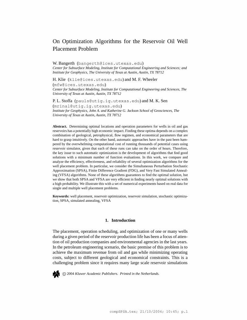
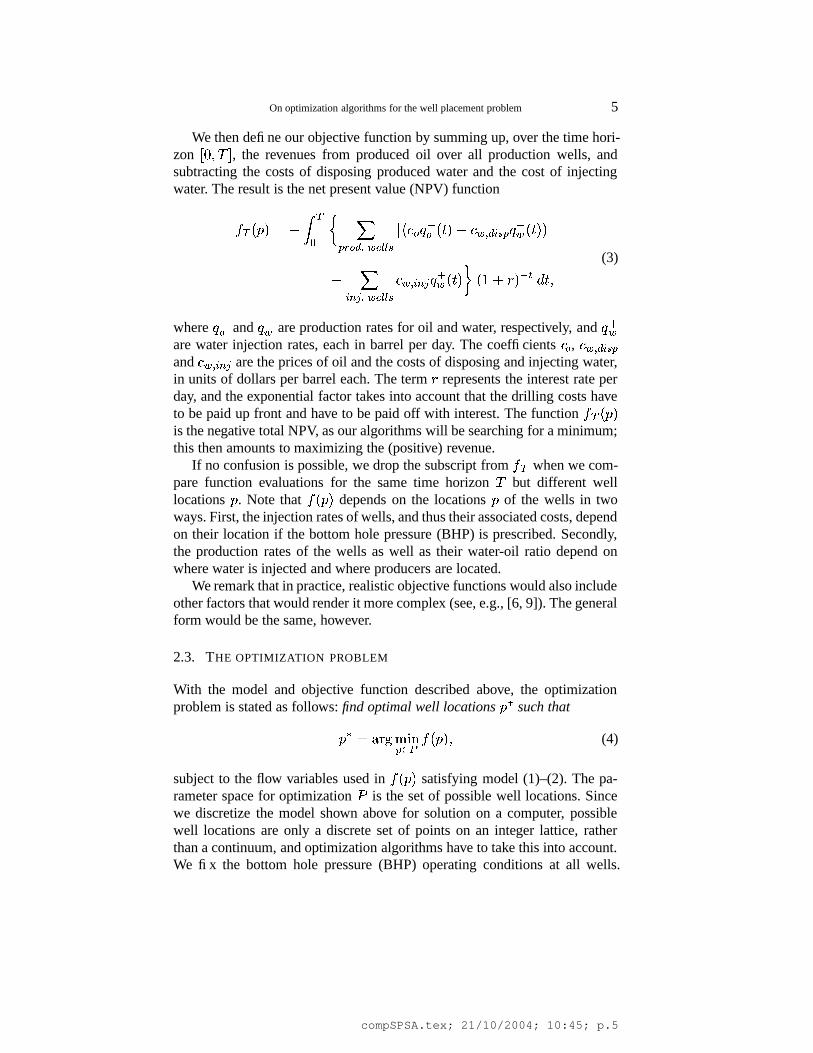
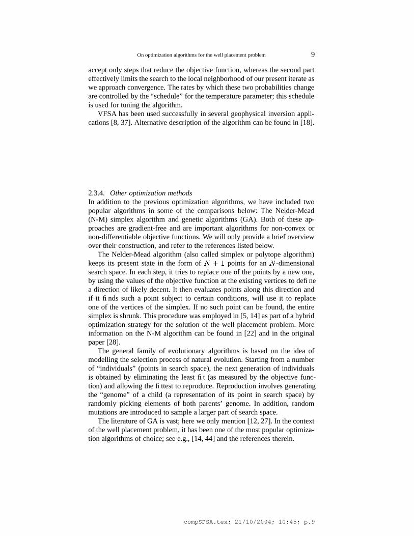
Figure 1. Permeability field showing the positions of current wells. The symbols ‘ � ’ and ‘�

’indicate injection and producer wells, respectively.

3. Results for placement of a single well

3.1. THE RESERVOIR MODEL

We consider a relatively simple 2D reservoir� � � � ��

� � �� 2 ?� � ofroughly 25 million ft � , which is discretized by

� 2�� spatial grid blocks of

��

ft length along each horizontal direction, and a depth of �

ft. Within thisreservoir, we fix the location of five wells (two injectors and three producers,see Fig. 1) and want to optimize the location of a third injector well. Sincethe model consists of 3904 grid blocks, the set of possible well locations overwhich we optimize is the integer lattice ) � � � � � 2 ?� � ?� � � � � � ��

�� 2 ?� � ?� � � � � � ��

of cell midpoints. The reservoir under study is lo-cated at a depth of 1 km ( ��

��ft) and corresponds to a 2D section extracted

from the Gulf of Mexico. The porosity has been fixed at� � � �

but thereservoir has a heterogeneous permeability field as shown in Figure 1. Therelative permeability and capillary pressure curves correspond to a single typeof rock. The reservoir is assumed to be surrounded by impermeable rock; thatis, fluxes are zero at the boundary. The fluids are initially in equilibrium withwater pressures set to 2600 psi and oil saturation to

� ��. For this initial case,

an opposite-corner well distribution was defined as shown in Figure 1.For the objective function (3), cost coefficients were chosen as follows:" � �

� , " �%$ �'& �#� � 2�� and " �/$ &,+�- �

. We chose an interest rate 3 of2 �� F2

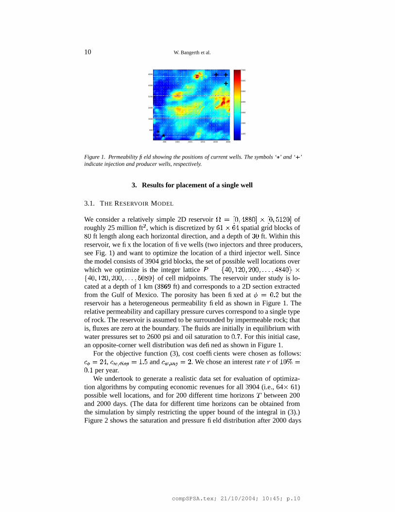
per year.We undertook to generate a realistic data set for evaluation of optimiza-

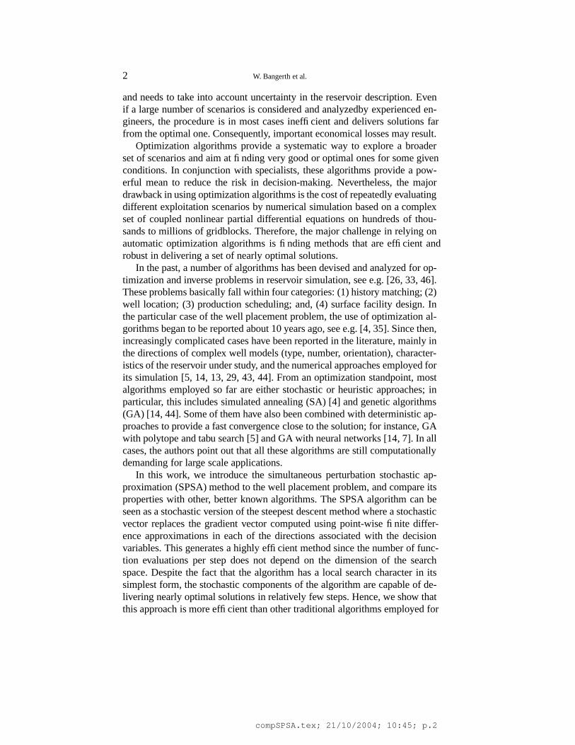
tion algorithms by computing economic revenues for all 3904 (i.e., 64 � 61)possible well locations, and for 200 different time horizons � between 200and 2000 days. (The data for different time horizons can be obtained fromthe simulation by simply restricting the upper bound of the integral in (3).)Figure 2 shows the saturation and pressure field distribution after 2000 days

compSPSA.tex; 21/10/2004; 10:45; p.10


800 1600 2400 3200 4000 4800

800

1600

2400

3200

4000

4800

0.25

0.3

0.35

0.4

0.45

0.5

0.55

0.6

0.65

0.7

800 1600 2400 3200 4000 4800

800

1600

2400

3200

4000

4800

2400

2450

2500

2550

2600

2650

2700

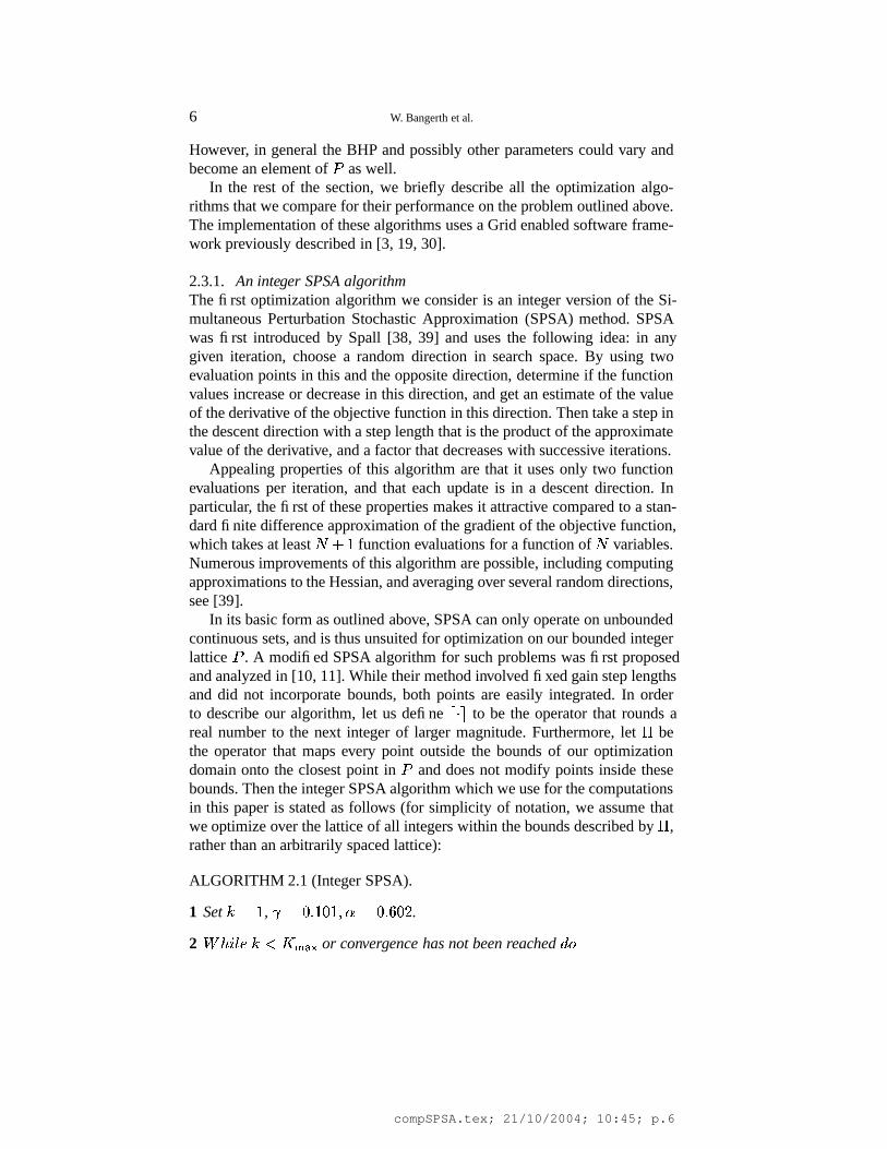
Figure 2. Left: Oil saturation at the end of the simulation for the original distribution of fivewells. Right: Oil pressure.

800 1600 2400 3200 4000 4800

800

1600

2400

3200

4000

4800

3

4

5

6

7

8

9

10

x 107

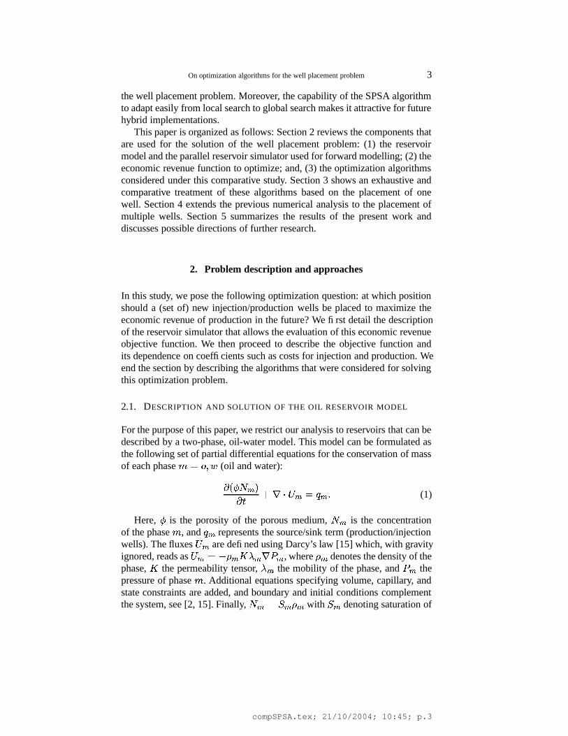
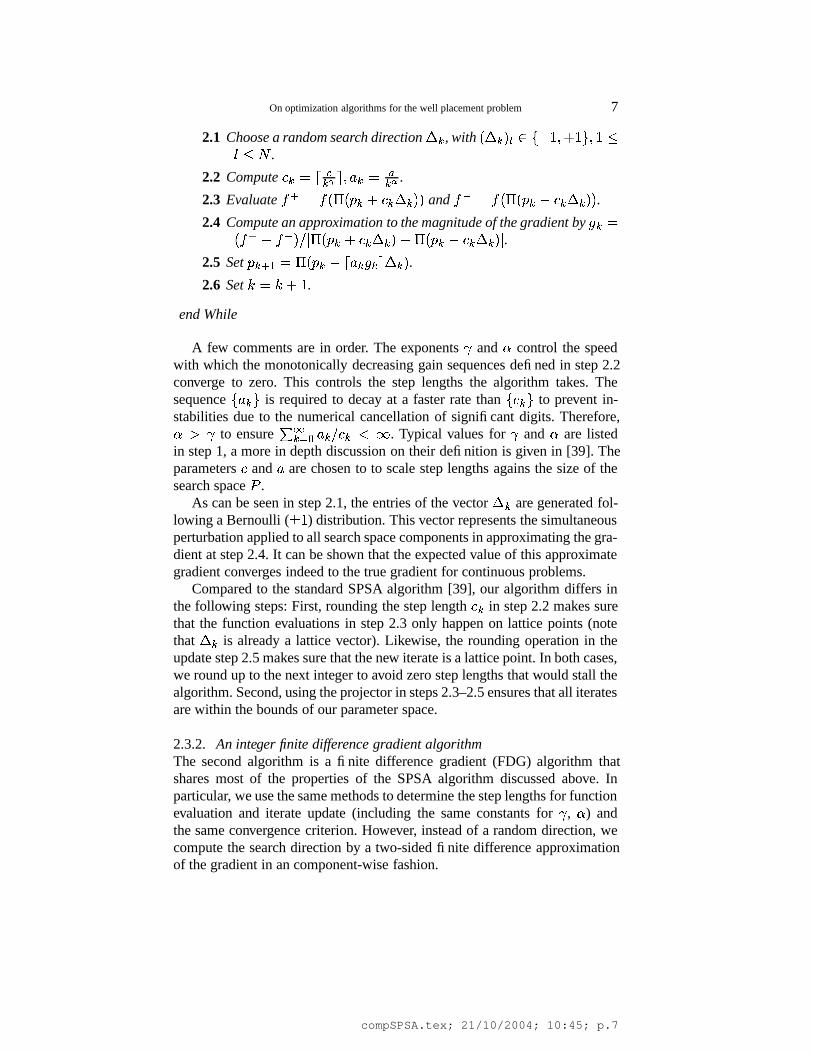
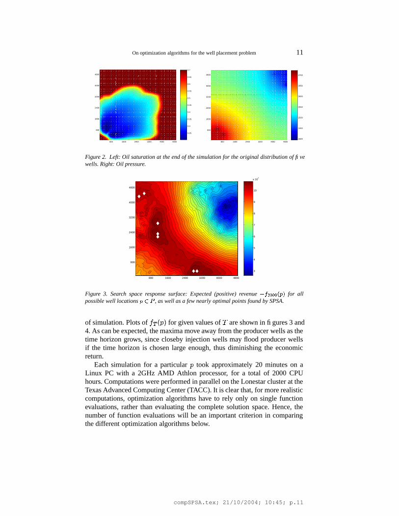
Figure 3. Search space response surface: Expected (positive) revenue ��

for allpossible well locations

� ��, as well as a few nearly optimal points found by SPSA.

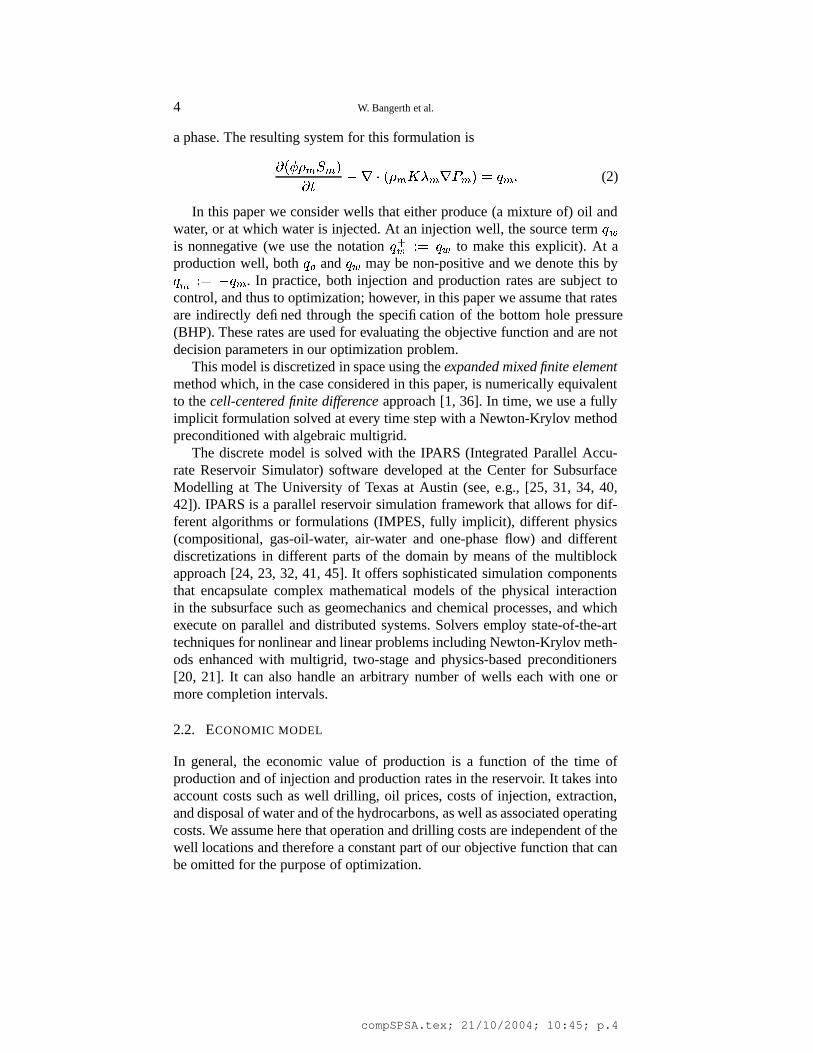
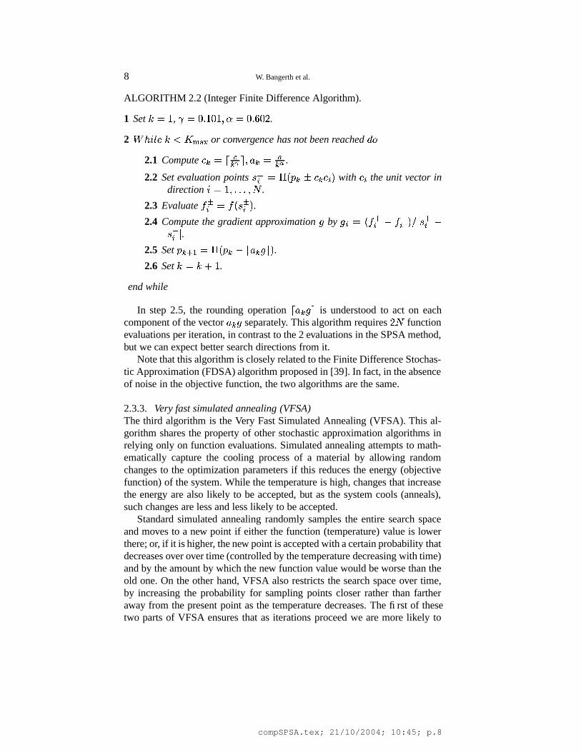
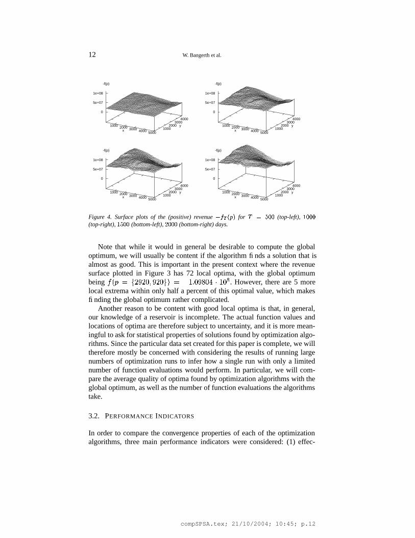
of simulation. Plots of� � � �

for given values of � are shown in figures 3 and4. As can be expected, the maxima move away from the producer wells as thetime horizon grows, since closeby injection wells may flood producer wellsif the time horizon is chosen large enough, thus diminishing the economicreturn.

Each simulation for a particular

took approximately 20 minutes on aLinux PC with a 2GHz AMD Athlon processor, for a total of 2000 CPUhours. Computations were performed in parallel on the Lonestar cluster at theTexas Advanced Computing Center (TACC). It is clear that, for more realisticcomputations, optimization algorithms have to rely only on single functionevaluations, rather than evaluating the complete solution space. Hence, thenumber of function evaluations will be an important criterion in comparingthe different optimization algorithms below.

compSPSA.tex; 21/10/2004; 10:45; p.11


1000 2000 3000 4000 5000x 1000

2000 3000

4000

y

0

5e+07

1e+08

-f(p)

1000 2000 3000 4000 5000x 1000

2000 3000

4000

y

0

5e+07

1e+08

-f(p)

1000 2000 3000 4000 5000x 1000

2000 3000

4000

y

0

5e+07

1e+08

-f(p)

1000 2000 3000 4000 5000x 1000

2000 3000

4000

y

0

5e+07

1e+08

-f(p)

Figure 4. Surface plots of the (positive) revenue ��

for��

(top-left), � ��(top-right), � �� (bottom-left), �� (bottom-right) days.

Note that while it would in general be desirable to compute the globaloptimum, we will usually be content if the algorithm finds a solution that isalmost as good. This is important in the present context where the revenuesurface plotted in Figure 3 has 72 local optima, with the global optimumbeing

� � � � � ?� � � ?� � � � ! 2�� 2 �� . However, there are 5 morelocal extrema within only half a percent of this optimal value, which makesfinding the global optimum rather complicated.

Another reason to be content with good local optima is that, in general,our knowledge of a reservoir is incomplete. The actual function values andlocations of optima are therefore subject to uncertainty, and it is more mean-ingful to ask for statistical properties of solutions found by optimization algo-rithms. Since the particular data set created for this paper is complete, we willtherefore mostly be concerned with considering the results of running largenumbers of optimization runs to infer how a single run with only a limitednumber of function evaluations would perform. In particular, we will com-pare the average quality of optima found by optimization algorithms with theglobal optimum, as well as the number of function evaluations the algorithmstake.

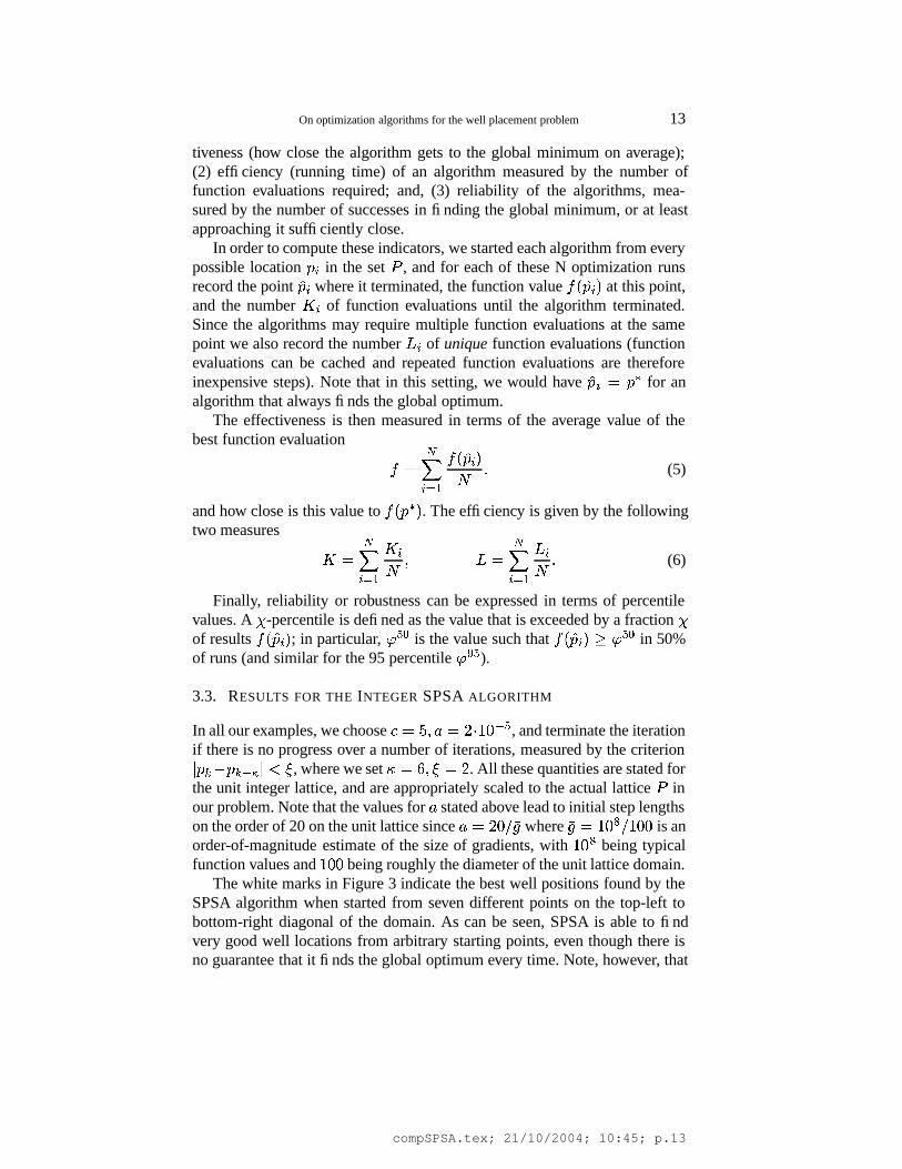
3.2. PERFORMANCE INDICATORS

In order to compare the convergence properties of each of the optimizationalgorithms, three main performance indicators were considered: (1) effec-

compSPSA.tex; 21/10/2004; 10:45; p.12


tiveness (how close the algorithm gets to the global minimum on average);(2) efficiency (running time) of an algorithm measured by the number offunction evaluations required; and, (3) reliability of the algorithms, mea-sured by the number of successes in finding the global minimum, or at leastapproaching it sufficiently close.

In order to compute these indicators, we started each algorithm from everypossible location

& in the set ) , and for each of these N optimization runsrecord the point � & where it terminated, the function value

� � & � at this point,and the number

$ & of function evaluations until the algorithm terminated.Since the algorithms may require multiple function evaluations at the samepoint we also record the number

� & of unique function evaluations (functionevaluations can be cached and repeated function evaluations are thereforeinexpensive steps). Note that in this setting, we would have � & � ;

for analgorithm that always finds the global optimum.

The effectiveness is then measured in terms of the average value of thebest function evaluation

�� & ) �� & ��

(5)

and how close is this value to� � ; �

. The efficiency is given by the followingtwo measures

�$ ��& ) �$ &� � ��

�� & ) �� &� � (6)

Finally, reliability or robustness can be expressed in terms of percentilevalues. A � -percentile is defined as the value that is exceeded by a fraction �of results

� � & � ; in particular, ��

is the value such that� � & ��

in 50%

of runs (and similar for the 95 percentile �� ).

3.3. RESULTS FOR THE INTEGER SPSA ALGORITHM

In all our examples, we choose " � ��*� � 2 � � � , and terminate the iterationif there is no progress over a number of iterations, measured by the criterion� �+! �

�� , where we set � � � ��

. All these quantities are stated forthe unit integer lattice, and are appropriately scaled to the actual lattice ) inour problem. Note that the values for � stated above lead to initial step lengthson the order of 20 on the unit lattice since �*� ?� � �� where

��*� 2 � � � 2 � �is an

order-of-magnitude estimate of the size of gradients, with2 � �

being typicalfunction values and

2 � �being roughly the diameter of the unit lattice domain.

The white marks in Figure 3 indicate the best well positions found by theSPSA algorithm when started from seven different points on the top-left tobottom-right diagonal of the domain. As can be seen, SPSA is able to findvery good well locations from arbitrary starting points, even though there isno guarantee that it finds the global optimum every time. Note, however, that

compSPSA.tex; 21/10/2004; 10:45; p.13


1000 2000 3000 4000 5000x 1000

2000 3000

4000

y

0

0.05

0.1

0.15

1000 2000 3000 4000 5000x 1000

2000 3000

4000

y

0

0.05

0.1

0.15

1000 2000 3000 4000 5000x 1000

2000 3000

4000

y

0

0.05

0.1

0.15

1000 2000 3000 4000 5000x 1000

2000 3000

4000

y

0

0.05

0.1

0.15

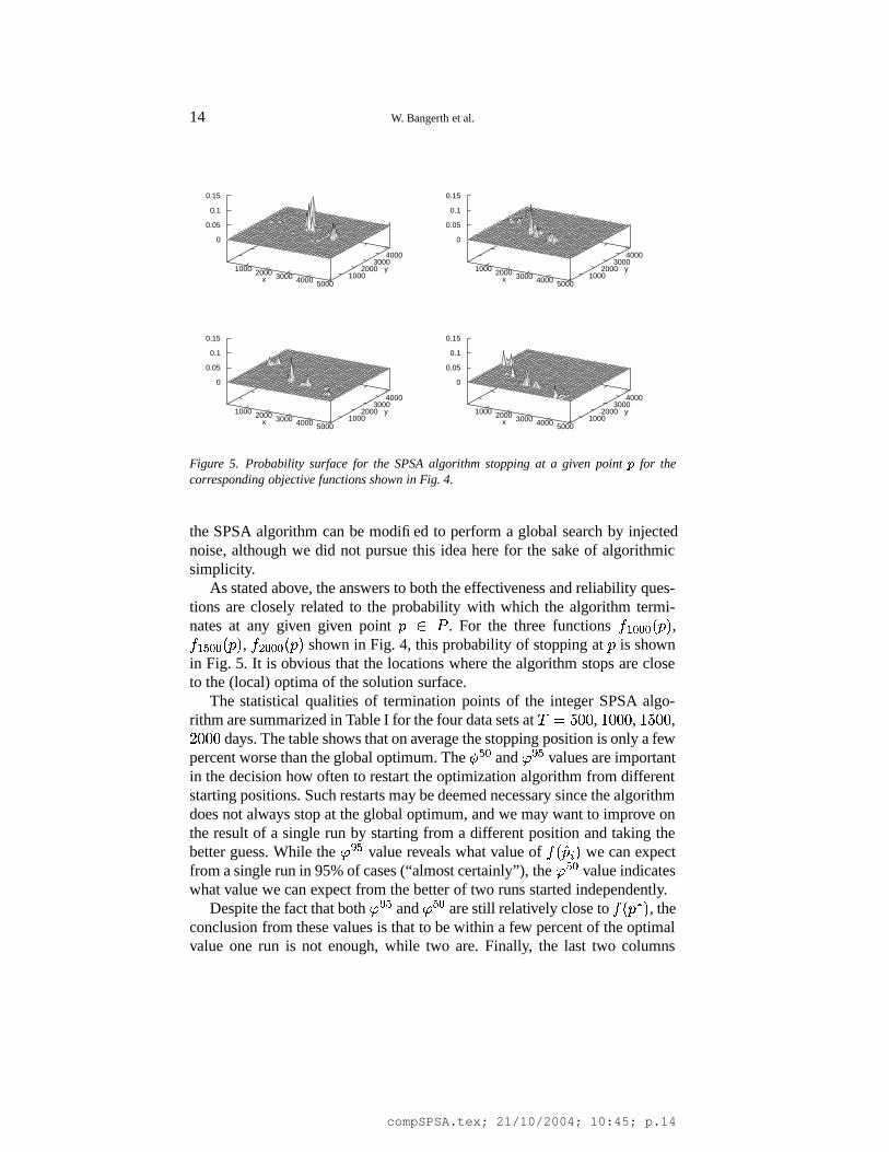
Figure 5. Probability surface for the SPSA algorithm stopping at a given point

for thecorresponding objective functions shown in Fig. 4.

the SPSA algorithm can be modified to perform a global search by injectednoise, although we did not pursue this idea here for the sake of algorithmicsimplicity.

As stated above, the answers to both the effectiveness and reliability ques-tions are closely related to the probability with which the algorithm termi-nates at any given given point

� ) . For the three functions� � ' ' � � ,� � � ' � � , � � ' ' � � shown in Fig. 4, this probability of stopping at

is shown

in Fig. 5. It is obvious that the locations where the algorithm stops are closeto the (local) optima of the solution surface.

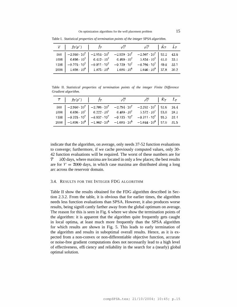
The statistical qualities of termination points of the integer SPSA algo-rithm are summarized in Table I for the four data sets at ��

� �,2 � � �

,2� �

,?� � �days. The table shows that on average the stopping position is only a few

percent worse than the global optimum. The� � and �� values are important

in the decision how often to restart the optimization algorithm from differentstarting positions. Such restarts may be deemed necessary since the algorithmdoes not always stop at the global optimum, and we may want to improve onthe result of a single run by starting from a different position and taking thebetter guess. While the � � � value reveals what value of

� � & � we can expectfrom a single run in 95% of cases (“almost certainly”), the � �

value indicates

what value we can expect from the better of two runs started independently.Despite the fact that both � � � and � �

are still relatively close to

� � ; �, the

conclusion from these values is that to be within a few percent of the optimalvalue one run is not enough, while two are. Finally, the last two columns

compSPSA.tex; 21/10/2004; 10:45; p.14


Table I. Statistical properties of termination points of the integer SPSA algorithm.

� � � � � � ��

� ��

Table II. Statistical properties of termination points of the integer Finite DifferenceGradient algorithm.

� � � � � � ��

� ��

indicate that the algorithm, on average, only needs 37-52 function evaluationsto converge; furthermore, if we cache previously computed values, only 30-42 function evaluations will be required. The worst of these numbers are for��

� �days, where maxima are located in only a few places; the best results

are for � � ?� � �days, in which case maxima are distributed along a long

arc across the reservoir domain.

3.4. RESULTS FOR THE INTEGER FDG ALGORITHM

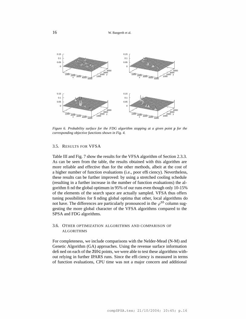
Table II show the results obtained for the FDG algorithm described in Sec-tion 2.3.2. From the table, it is obvious that for earlier times, the algorithmneeds less function evaluations than SPSA. However, it also produces worseresults, being significantly farther away from the global optimum on average.The reason for this is seen in Fig. 6 where we show the termination points ofthe algorithm: it is apparent that the algorithm quite frequently gets caughtin local optima, at least much more frequently than the SPSA algorithmfor which results are shown in Fig. 5. This leads to early termination ofthe algorithm and results in suboptimal overall results. Hence, as it is ex-pected from a non-convex or non-differentiable objective function, accurateor noise-free gradient computations does not necessarily lead to a high levelof effectiveness, efficiency and reliability in the search for a (nearly) globaloptimal solution.

compSPSA.tex; 21/10/2004; 10:45; p.15


1000 2000 3000 4000 5000x 1000

2000 3000

4000

y

0

0.05

0.1

0.15

1000 2000 3000 4000 5000x 1000

2000 3000

4000

y

0

0.05

0.1

0.15

1000 2000 3000 4000 5000x 1000

2000 3000

4000

y

0

0.05

0.1

0.15

1000 2000 3000 4000 5000x 1000

2000 3000

4000

y

0

0.05

0.1

0.15

Figure 6. Probability surface for the FDG algorithm stopping at a given point

for thecorresponding objective functions shown in Fig. 4.

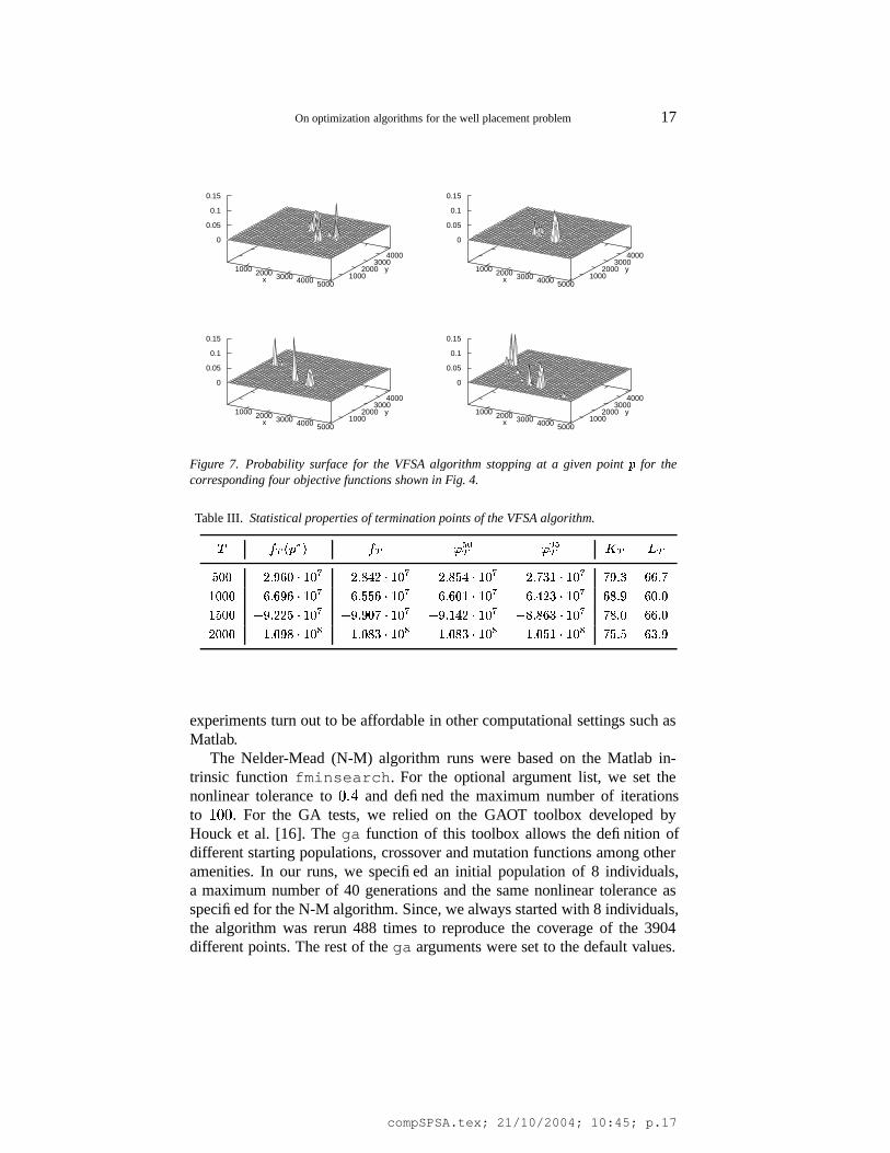
3.5. RESULTS FOR VFSA

Table III and Fig. 7 show the results for the VFSA algorithm of Section 2.3.3.As can be seen from the table, the results obtained with this algorithm aremore reliable and effective than for the other methods, albeit at the cost ofa higher number of function evaluations (i.e., poor efficiency). Nevertheless,these results can be further improved: by using a stretched cooling schedule(resulting in a further increase in the number of function evaluations) the al-gorithm find the global optimum in 95% of our runs even though only 10-15%of the elements of the search space are actually sampled. VFSA thus offerstuning possibilities for finding global optima that other, local algorithms donot have. The differences are particularly pronounced in the � � � column sug-gesting the more global character of the VFSA algorithms compared to theSPSA and FDG algorithms.

3.6. OTHER OPTIMIZATION ALGORITHMS AND COMPARISON OF

ALGORITHMS

For completeness, we include comparisons with the Nelder-Mead (N-M) andGenetic Algorithm (GA) approaches. Using the revenue surface informationdefined on each of the

� �� points, we were able to test these algorithms with-

out relying in further IPARS runs. Since the efficiency is measured in termsof function evaluations, CPU time was not a major concern and additional

compSPSA.tex; 21/10/2004; 10:45; p.16


1000 2000 3000 4000 5000x 1000

2000 3000

4000

y

0

0.05

0.1

0.15

1000 2000 3000 4000 5000x 1000

2000 3000

4000

y

0

0.05

0.1

0.15

1000 2000 3000 4000 5000x 1000

2000 3000

4000

y

0

0.05

0.1

0.15

1000 2000 3000 4000 5000x 1000

2000 3000

4000

y

0

0.05

0.1

0.15

Figure 7. Probability surface for the VFSA algorithm stopping at a given point

for thecorresponding four objective functions shown in Fig. 4.

Table III. Statistical properties of termination points of the VFSA algorithm.

� � � � � � ��

� ��

experiments turn out to be affordable in other computational settings such asMatlab.

The Nelder-Mead (N-M) algorithm runs were based on the Matlab in-trinsic function fminsearch. For the optional argument list, we set thenonlinear tolerance to

� �� and defined the maximum number of iterations

to2 � �

. For the GA tests, we relied on the GAOT toolbox developed byHouck et al. [16]. The ga function of this toolbox allows the definition ofdifferent starting populations, crossover and mutation functions among otheramenities. In our runs, we specified an initial population of 8 individuals,a maximum number of 40 generations and the same nonlinear tolerance asspecified for the N-M algorithm. Since, we always started with 8 individuals,the algorithm was rerun 488 times to reproduce the coverage of the 3904different points. The rest of the ga arguments were set to the default values.

compSPSA.tex; 21/10/2004; 10:45; p.17


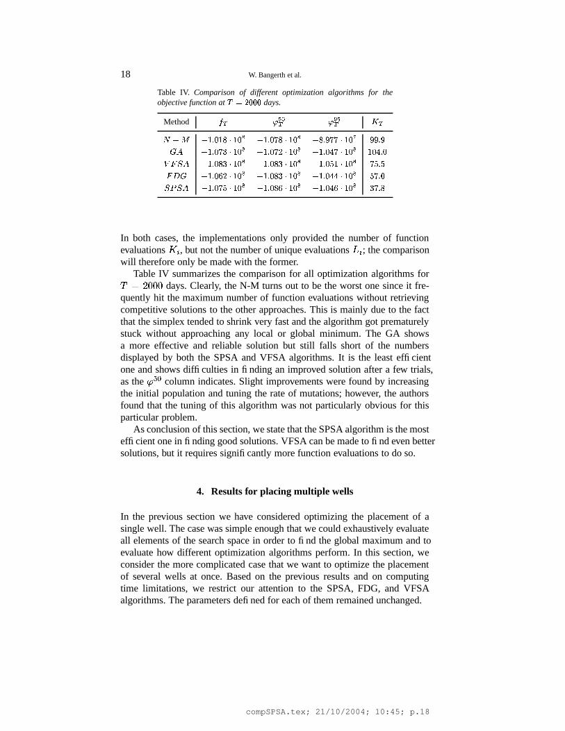
Table IV. Comparison of different optimization algorithms for theobjective function at

� � �� days.

Method��

� ��

� ��

In both cases, the implementations only provided the number of functionevaluations

$ & , but not the number of unique evaluations� & ; the comparison

will therefore only be made with the former.Table IV summarizes the comparison for all optimization algorithms for� � ?� � �

days. Clearly, the N-M turns out to be the worst one since it fre-quently hit the maximum number of function evaluations without retrievingcompetitive solutions to the other approaches. This is mainly due to the factthat the simplex tended to shrink very fast and the algorithm got prematurelystuck without approaching any local or global minimum. The GA showsa more effective and reliable solution but still falls short of the numbersdisplayed by both the SPSA and VFSA algorithms. It is the least efficientone and shows difficulties in finding an improved solution after a few trials,as the � �

column indicates. Slight improvements were found by increasing

the initial population and tuning the rate of mutations; however, the authorsfound that the tuning of this algorithm was not particularly obvious for thisparticular problem.

As conclusion of this section, we state that the SPSA algorithm is the mostefficient one in finding good solutions. VFSA can be made to find even bettersolutions, but it requires significantly more function evaluations to do so.

4. Results for placing multiple wells

In the previous section we have considered optimizing the placement of asingle well. The case was simple enough that we could exhaustively evaluateall elements of the search space in order to find the global maximum and toevaluate how different optimization algorithms perform. In this section, weconsider the more complicated case that we want to optimize the placementof several wells at once. Based on the previous results and on computingtime limitations, we restrict our attention to the SPSA, FDG, and VFSAalgorithms. The parameters defined for each of them remained unchanged.

compSPSA.tex; 21/10/2004; 10:45; p.18


800 1600 2400 3200 4000 4800

800

1600

2400

3200

4000

4800

5

6

7

8

9

10

11

12

x 107

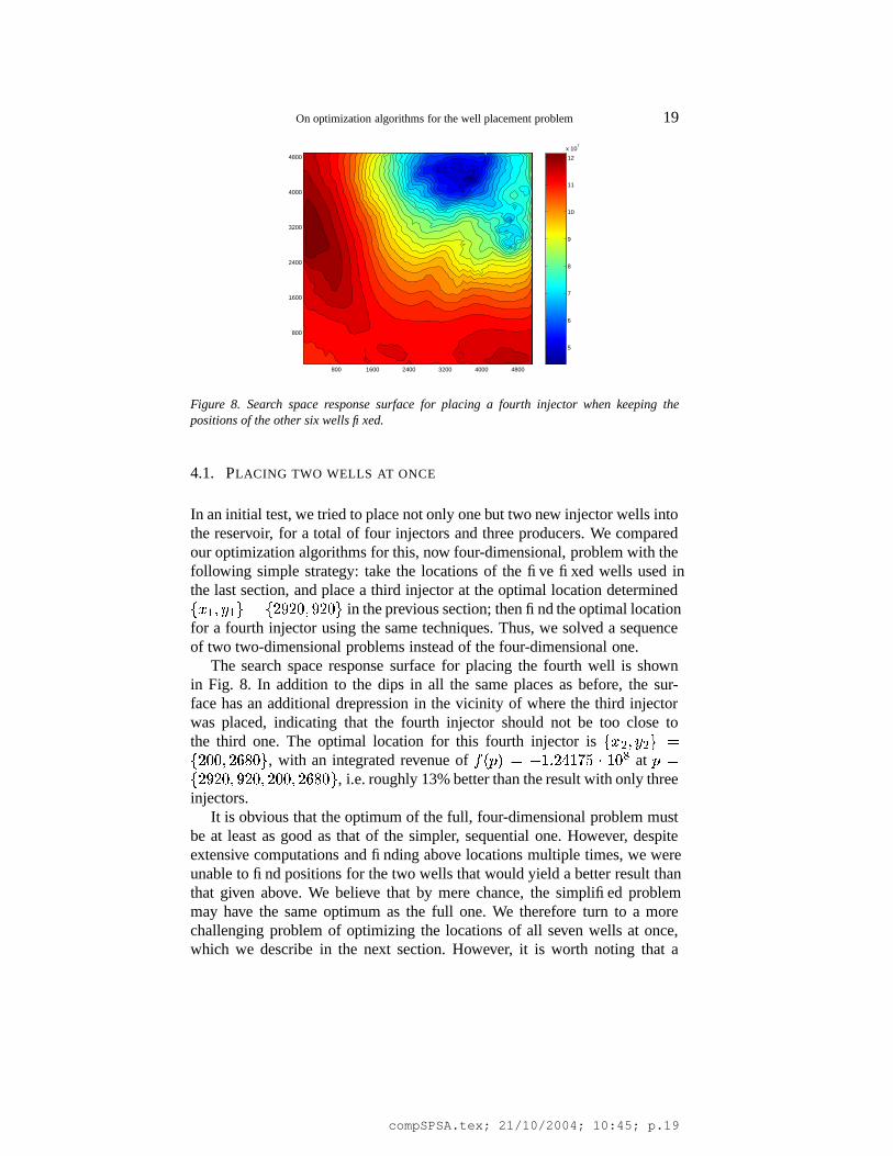
Figure 8. Search space response surface for placing a fourth injector when keeping thepositions of the other six wells fixed.

4.1. PLACING TWO WELLS AT ONCE

In an initial test, we tried to place not only one but two new injector wells intothe reservoir, for a total of four injectors and three producers. We comparedour optimization algorithms for this, now four-dimensional, problem with thefollowing simple strategy: take the locations of the five fixed wells used inthe last section, and place a third injector at the optimal location determined�� ?� � � ?� �

in the previous section; then find the optimal locationfor a fourth injector using the same techniques. Thus, we solved a sequenceof two two-dimensional problems instead of the four-dimensional one.

The search space response surface for placing the fourth well is shownin Fig. 8. In addition to the dips in all the same places as before, the sur-face has an additional drepression in the vicinity of where the third injectorwas placed, indicating that the fourth injector should not be too close tothe third one. The optimal location for this fourth injector is ��

� �� ?� � � � � � �

, with an integrated revenue of� � � � ! 2�� 2 � � 2 � � at

�� ?� � � ?� � ?� � � � � � �

, i.e. roughly 13% better than the result with only threeinjectors.

It is obvious that the optimum of the full, four-dimensional problem mustbe at least as good as that of the simpler, sequential one. However, despiteextensive computations and finding above locations multiple times, we wereunable to find positions for the two wells that would yield a better result thanthat given above. We believe that by mere chance, the simplified problemmay have the same optimum as the full one. We therefore turn to a morechallenging problem of optimizing the locations of all seven wells at once,which we describe in the next section. However, it is worth noting that a

compSPSA.tex; 21/10/2004; 10:45; p.19


f(p)=-1.65044e8

x

x

x

oo

o

o

f(p)=-1.64713e8

x

x

x

o

o

o

o

f(p)=-1.63116e8

x

x

xo

o

o

o

f(p)=-1.59290e8

x

x

x

o

o

o

o

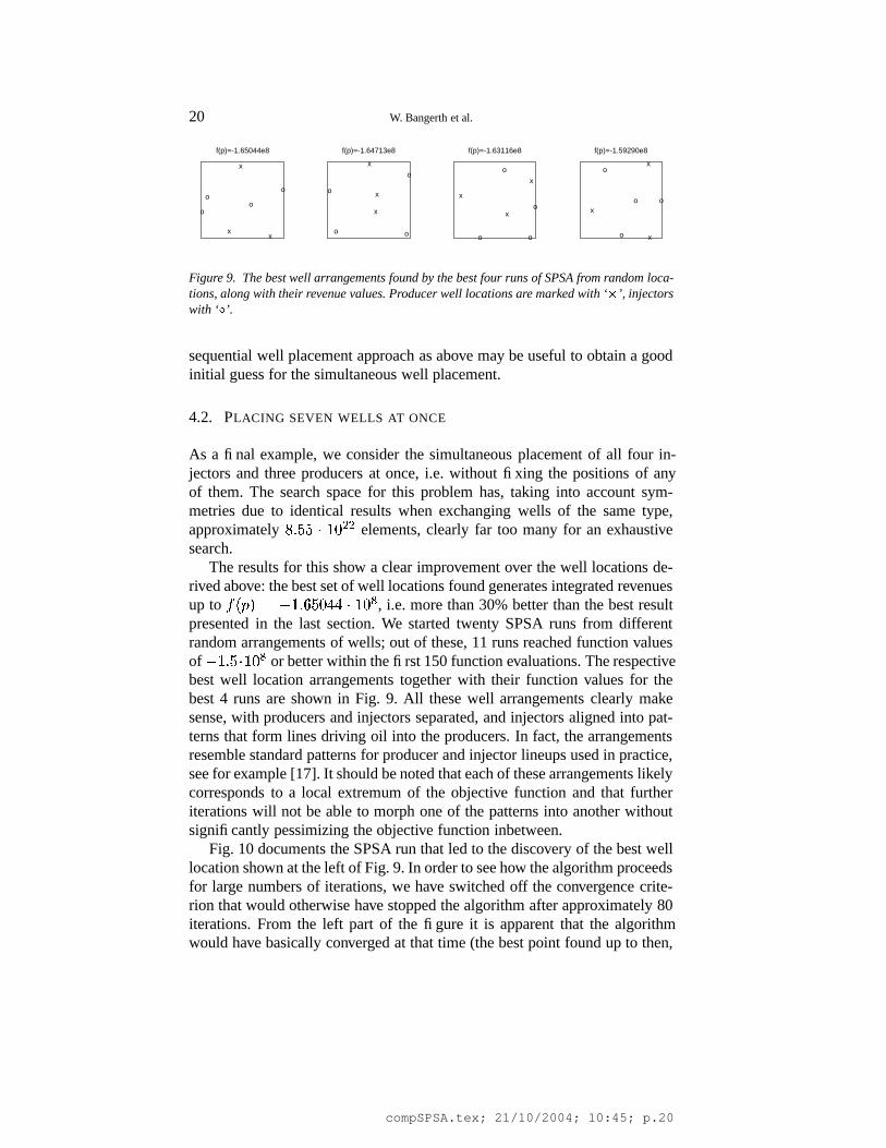
Figure 9. The best well arrangements found by the best four runs of SPSA from random loca-tions, along with their revenue values. Producer well locations are marked with ‘ � ’, injectorswith ‘ � ’.

sequential well placement approach as above may be useful to obtain a goodinitial guess for the simultaneous well placement.

4.2. PLACING SEVEN WELLS AT ONCE

As a final example, we consider the simultaneous placement of all four in-jectors and three producers at once, i.e. without fixing the positions of anyof them. The search space for this problem has, taking into account sym-metries due to identical results when exchanging wells of the same type,approximately �

�� 2 � �� elements, clearly far too many for an exhaustive

search.The results for this show a clear improvement over the well locations de-

rived above: the best set of well locations found generates integrated revenuesup to

� � � � ! 2�� 2 � � , i.e. more than 30% better than the best resultpresented in the last section. We started twenty SPSA runs from differentrandom arrangements of wells; out of these, 11 runs reached function valuesof ! 2�� 2 � � or better within the first 150 function evaluations. The respectivebest well location arrangements together with their function values for thebest 4 runs are shown in Fig. 9. All these well arrangements clearly makesense, with producers and injectors separated, and injectors aligned into pat-terns that form lines driving oil into the producers. In fact, the arrangementsresemble standard patterns for producer and injector lineups used in practice,see for example [17]. It should be noted that each of these arrangements likelycorresponds to a local extremum of the objective function and that furtheriterations will not be able to morph one of the patterns into another withoutsignificantly pessimizing the objective function inbetween.

Fig. 10 documents the SPSA run that led to the discovery of the best welllocation shown at the left of Fig. 9. In order to see how the algorithm proceedsfor large numbers of iterations, we have switched off the convergence crite-rion that would otherwise have stopped the algorithm after approximately 80iterations. From the left part of the figure it is apparent that the algorithmwould have basically converged at that time (the best point found up to then,

compSPSA.tex; 21/10/2004; 10:45; p.20


-1.8e+08

-1.6e+08

-1.4e+08

-1.2e+08

-1e+08

-8e+07

-6e+07

-4e+07

-2e+07

0

0 50 100 150 200 250

f(p)

Number of function evaluation

Evaluation 0

xx

x

oo

o

o

Evaluation 10

x

x

x

o

ooo

Evaluation 20

x

x

x

oo

o

o

Evaluation 30

x

x

x

o o

o

o

Evaluation 40

x

x

x

o o

o

o

Evaluation 50

x

x

x

o o

o

o

Evaluation 60

x

x

x

o o

o

o

Evaluation 70

x

x

x

o oo

o

Evaluation 80

x

x

x

oo

o

o

Evaluation 90

x

x

x

oo

o

o

Evaluation 100

x

x

x

oo

o

o

Evaluation 200

x

x

x

o oo

o

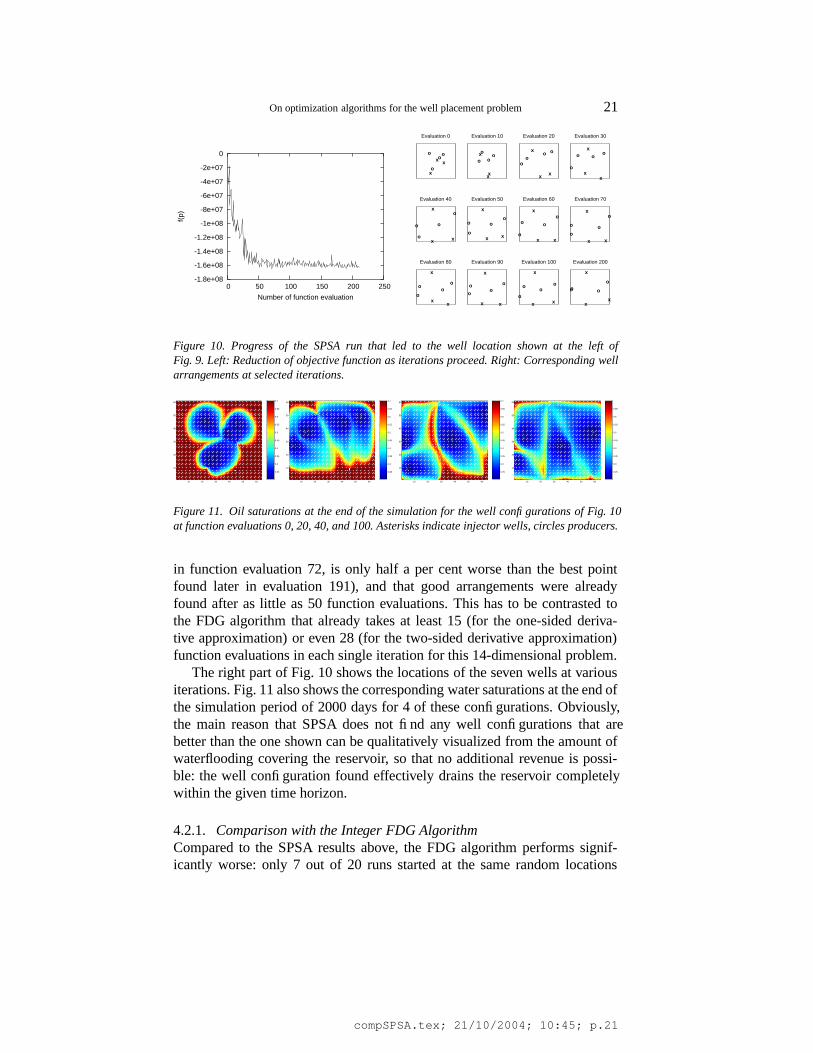
Figure 10. Progress of the SPSA run that led to the well location shown at the left ofFig. 9. Left: Reduction of objective function as iterations proceed. Right: Corresponding wellarrangements at selected iterations.

10 20 30 40 50 60

10

20

30

40

50

60

0.25

0.3

0.35

0.4

0.45

0.5

0.55

0.6

0.65

0.7

10 20 30 40 50 60

10

20

30

40

50

60

0.25

0.3

0.35

0.4

0.45

0.5

0.55

0.6

0.65

0.7

10 20 30 40 50 60

10

20

30

40

50

60

0.25

0.3

0.35

0.4

0.45

0.5

0.55

0.6

0.65

0.7

10 20 30 40 50 60

10

20

30

40

50

60

0.25

0.3

0.35

0.4

0.45

0.5

0.55

0.6

0.65

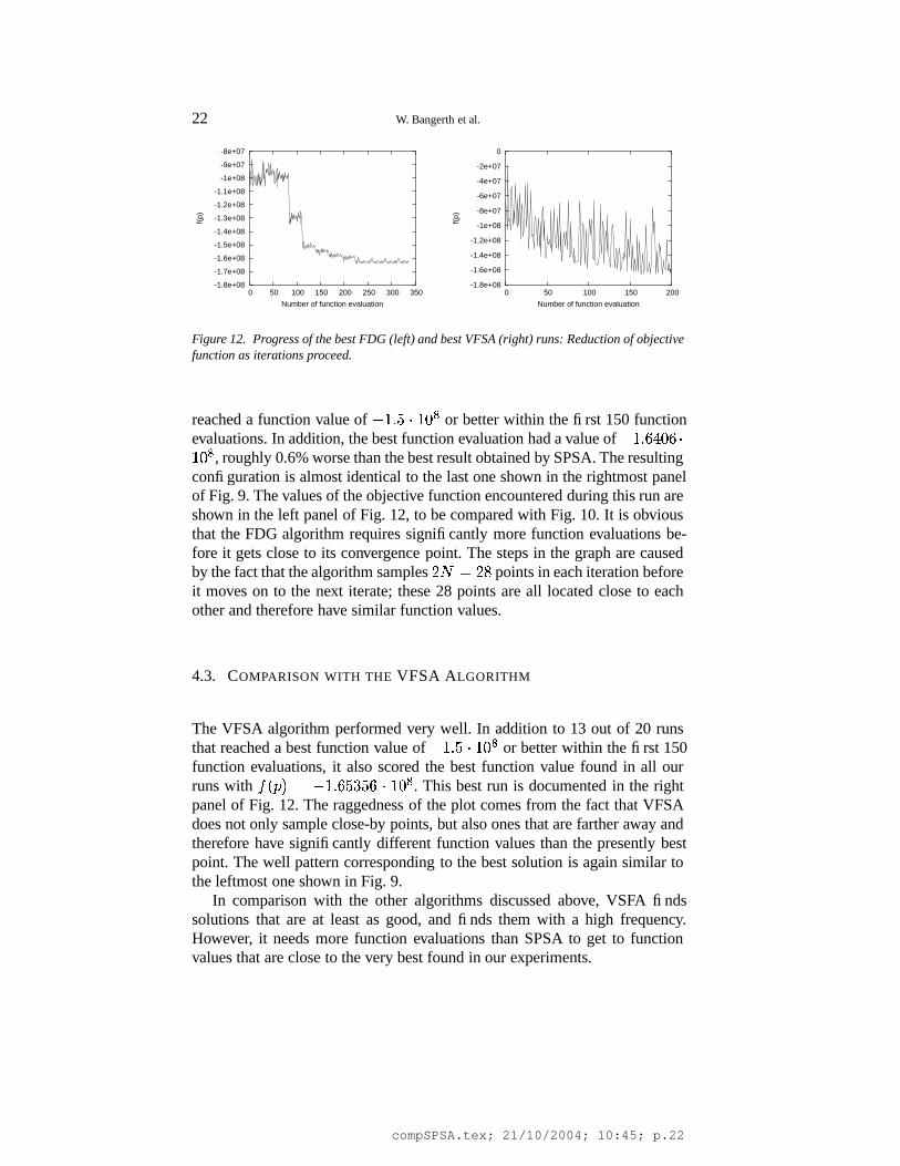
Figure 11. Oil saturations at the end of the simulation for the well configurations of Fig. 10at function evaluations 0, 20, 40, and 100. Asterisks indicate injector wells, circles producers.

in function evaluation 72, is only half a per cent worse than the best pointfound later in evaluation 191), and that good arrangements were alreadyfound after as little as 50 function evaluations. This has to be contrasted tothe FDG algorithm that already takes at least 15 (for the one-sided deriva-tive approximation) or even 28 (for the two-sided derivative approximation)function evaluations in each single iteration for this 14-dimensional problem.

The right part of Fig. 10 shows the locations of the seven wells at variousiterations. Fig. 11 also shows the corresponding water saturations at the end ofthe simulation period of 2000 days for 4 of these configurations. Obviously,the main reason that SPSA does not find any well configurations that arebetter than the one shown can be qualitatively visualized from the amount ofwaterflooding covering the reservoir, so that no additional revenue is possi-ble: the well configuration found effectively drains the reservoir completelywithin the given time horizon.

4.2.1. Comparison with the Integer FDG AlgorithmCompared to the SPSA results above, the FDG algorithm performs signif-icantly worse: only 7 out of 20 runs started at the same random locations

compSPSA.tex; 21/10/2004; 10:45; p.21


-1.8e+08

-1.7e+08

-1.6e+08

-1.5e+08

-1.4e+08

-1.3e+08

-1.2e+08

-1.1e+08

-1e+08

-9e+07

-8e+07

0 50 100 150 200 250 300 350

f(p)


-1.8e+08

-1.6e+08

-1.4e+08

-1.2e+08

-1e+08

-8e+07

-6e+07

-4e+07

-2e+07

0

0 50 100 150 200

f(p)


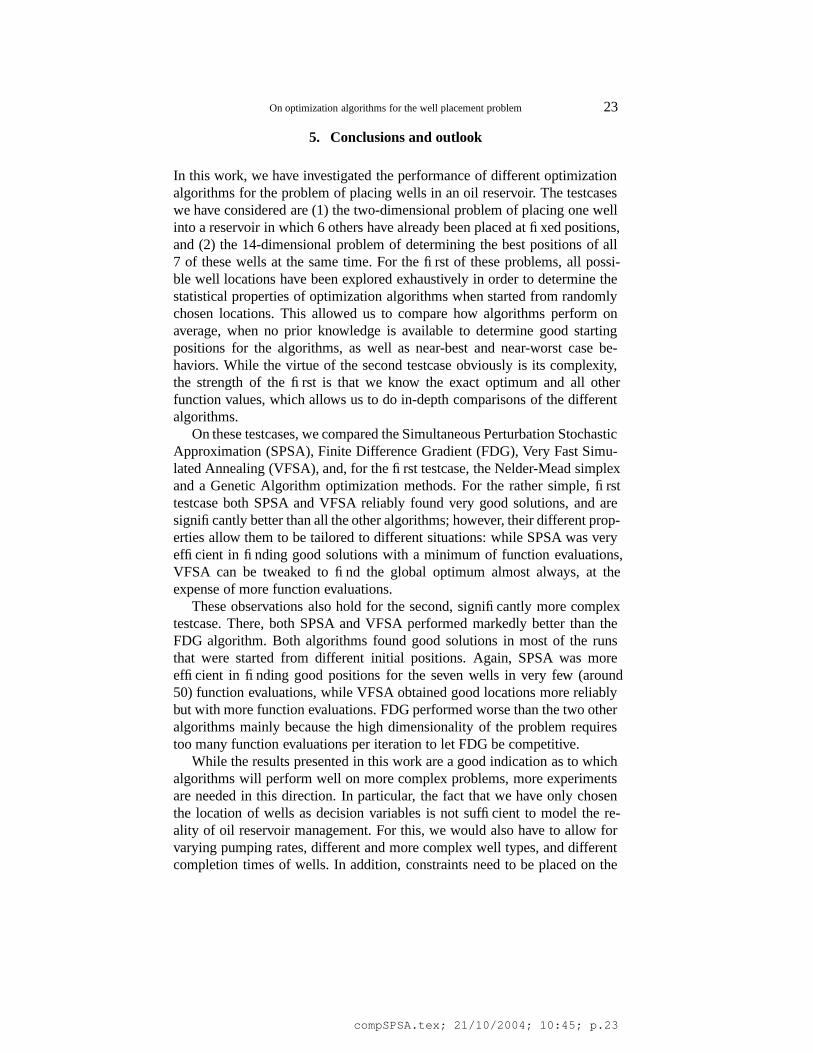
Figure 12. Progress of the best FDG (left) and best VFSA (right) runs: Reduction of objectivefunction as iterations proceed.

reached a function value of ! 2�� 2 � � or better within the first 150 functionevaluations. In addition, the best function evaluation had a value of ! 2�� 2 � �

, roughly 0.6% worse than the best result obtained by SPSA. The resultingconfiguration is almost identical to the last one shown in the rightmost panelof Fig. 9. The values of the objective function encountered during this run areshown in the left panel of Fig. 12, to be compared with Fig. 10. It is obviousthat the FDG algorithm requires significantly more function evaluations be-fore it gets close to its convergence point. The steps in the graph are causedby the fact that the algorithm samples

� � � points in each iteration before

it moves on to the next iterate; these 28 points are all located close to eachother and therefore have similar function values.

4.3. COMPARISON WITH THE VFSA ALGORITHM

The VFSA algorithm performed very well. In addition to 13 out of 20 runsthat reached a best function value of ! 2�� 2 � � or better within the first 150function evaluations, it also scored the best function value found in all ourruns with

� � � � ! 2�� 2 � � . This best run is documented in the rightpanel of Fig. 12. The raggedness of the plot comes from the fact that VFSAdoes not only sample close-by points, but also ones that are farther away andtherefore have significantly different function values than the presently bestpoint. The well pattern corresponding to the best solution is again similar tothe leftmost one shown in Fig. 9.

In comparison with the other algorithms discussed above, VSFA findssolutions that are at least as good, and finds them with a high frequency.However, it needs more function evaluations than SPSA to get to functionvalues that are close to the very best found in our experiments.

compSPSA.tex; 21/10/2004; 10:45; p.22


5. Conclusions and outlook

In this work, we have investigated the performance of different optimizationalgorithms for the problem of placing wells in an oil reservoir. The testcaseswe have considered are (1) the two-dimensional problem of placing one wellinto a reservoir in which 6 others have already been placed at fixed positions,and (2) the 14-dimensional problem of determining the best positions of all7 of these wells at the same time. For the first of these problems, all possi-ble well locations have been explored exhaustively in order to determine thestatistical properties of optimization algorithms when started from randomlychosen locations. This allowed us to compare how algorithms perform onaverage, when no prior knowledge is available to determine good startingpositions for the algorithms, as well as near-best and near-worst case be-haviors. While the virtue of the second testcase obviously is its complexity,the strength of the first is that we know the exact optimum and all otherfunction values, which allows us to do in-depth comparisons of the differentalgorithms.

On these testcases, we compared the Simultaneous Perturbation StochasticApproximation (SPSA), Finite Difference Gradient (FDG), Very Fast Simu-lated Annealing (VFSA), and, for the first testcase, the Nelder-Mead simplexand a Genetic Algorithm optimization methods. For the rather simple, firsttestcase both SPSA and VFSA reliably found very good solutions, and aresignificantly better than all the other algorithms; however, their different prop-erties allow them to be tailored to different situations: while SPSA was veryefficient in finding good solutions with a minimum of function evaluations,VFSA can be tweaked to find the global optimum almost always, at theexpense of more function evaluations.

These observations also hold for the second, significantly more complextestcase. There, both SPSA and VFSA performed markedly better than theFDG algorithm. Both algorithms found good solutions in most of the runsthat were started from different initial positions. Again, SPSA was moreefficient in finding good positions for the seven wells in very few (around50) function evaluations, while VFSA obtained good locations more reliablybut with more function evaluations. FDG performed worse than the two otheralgorithms mainly because the high dimensionality of the problem requirestoo many function evaluations per iteration to let FDG be competitive.

While the results presented in this work are a good indication as to whichalgorithms will perform well on more complex problems, more experimentsare needed in this direction. In particular, the fact that we have only chosenthe location of wells as decision variables is not sufficient to model the re-ality of oil reservoir management. For this, we would also have to allow forvarying pumping rates, different and more complex well types, and differentcompletion times of wells. In addition, constraints need to be placed on the

compSPSA.tex; 21/10/2004; 10:45; p.23


system, such as maximal and minimal capacities of surface facilities, and thereservoir description must be more complex than the relatively simple 2d casewe chose here in order to keep computing time within a range where differentalgorithms can be easily compared. Also, it will be interesting to investigatethe effects of uncertainty in the reservoir description on the performanceof algorithms; for example, we expect that averaging over several possiblerealizations of a stochastic reservoir model may smooth out the objectivefunction, which would probably aid the FDG algorithm more than the othermethods. Research in these directions is presently underway, and we willcontinue to investigate which algorithms are best suited for more complexand more realistic descriptions of the oil well placement problem.

Acknowledgments

The authors want to thank the National Science Foundation (NSF) for itssupport under the ITR grant EIA 0121523/EIA-0120934.

References

1. T. Arbogast, M. F. Wheeler, and I. Yotov. Mixed finite elements for elliptic prob-lems with tensor coefficients as cell-centered finite differences. SIAM J. Numer. Anal.,34(2):828–852, 1997.

2. K. Aziz and A. Settari. Petroleum Reservoir Simulation. Applied Science PublishersLtd., London, 1979.

3. W. Bangerth, H. Klie, V. Matossian, M. Parashar, and M. F. Wheeler. An autonomicreservoir framework for the stochastic optimization of well placement. Accepted forpublication in the Journal of ”Networks, Software Tools and Applications” from Kluwerin a special issue on Challenges of Large Applications in Distributed Environments,2004.

4. B. L. Becker and X. Song. Field development planning using simulated annealing-optimal economic well scheduling and placement. In SPE Annual Technical Conferenceand Exhibition, Dallas, Texas, October 1995. SPE 30650.

5. A. C. Bittencourt and R. N. Horne. Reservoir development and design optimization. InSPE Annual Technical Conference and Exhibition, San Antonio, Texas, October 1997.SPE 38895.

6. M. Carlson. Practical Reservoir Simulation. PennWell Corporation, 2003.7. A. Centilmen, T. Ertekin, and A. S. Grader. Applications of neural networks in multiwell

field development. In SPE Annual Technical Conference and Exhibition, Dallas, Texas,October 1999. SPE 56433.

8. R. K. Chunduru, M. Sen, and P. Stoffa. Hybrid optimization methods for geophysicalinversion. Goephysics, 62:1196–1207, 1997.

9. J. R. Fanchi. Principles of Applied Reservoir Simulation. Boston: Butterworth-Heinemann Gulf Professional Publishing, 2001. 2nd edition.

10. L. Gerencser, S. D. Hill, and Z. Vago. Optimization over discrete sets via SPSA. InProceedings of the 38th Conference on Decision and Control, Phoenix, AZ, 1999, pages1791–1795, 1999.

compSPSA.tex; 21/10/2004; 10:45; p.24


11. L. Gerencser, S. D. Hill, and Z. Vago. Discrete optimization via SPSA. In Proceedingsof the Americal Control Conference, Arlington, VA, 2001, pages 1503–1504, 2001.

12. D. Goldberg. Genetic Algorithms in Search, Optimization, and Machine Learning.Addison-Wesley, 1989.

13. B. Guyaguler. Optimization of Well Placement and Assesment of Uncertainty. PhDthesis, Stanford University, Department of Petroleum Engineering, 2002.

14. B. Guyaguler and R. N. Horne. Uncertainty assessment of well placement optimiza-tion. In SPE Annual Technical Conference and Exhibition, New Orleans, Louisiana,September, October 2001. SPE 71625.

15. R. Helmig. Multiphase flow and transport processes in the Subsurface. Springer, 1997.16. C. Houck, J. A. Joines, and M. G. Kay. A genetic algorithm for function optimization:

A Matlab implementation. Technical Report TR 95-09, North Carolina State University,1995.

17. N. Hyne. Nontechnical Guide to Petroleum Geology, Exploration, Drilling andProduction. Pennwell Books, 2nd edition, 2001.

18. L. Ingber. Very fast simulated reannealing. Math. Comput. Modeling, 12:967–993, 1989.19. H. Klie, W. Bangerth, M. F. Wheeler, M. Parashar, and V. Matossian. Parallel well

location optimization using stochastic algorithms on the grid computational framework.In 9th European Conference on the Mathematics of Oil Recovery, ECMOR, Cannes,France, August 30–September 2 2004. EAGE.

20. S. Lacroix, Y. Vassilevski, J. Wheeler, and M. F. Wheeler. Iterative solution methods formodelling multiphase flow in porous media fully implicitly. SIAM Journal of ScientificComputing, 25(3):905–926, 2003.

21. S. Lacroix, Y. Vassilevski, and M. F. Wheeler. Iterative solvers of the Implicit ParallelAccurate Reservoir Simulator (IPARS). Numerical Linear Algebra with Applications,4:537–549, 2001.

22. J. C. Lagarias, J. A. Reeds, M. H. Wright, and P. E. Wright. Convergence behavior of theNelder-Mead simplex algorithm in low dimensions. SIAM J. Optim., 9:112–147, 1999.

23. Q. Lu. A Parallel Multi-Block / Multi-Physics Approach for Multi-Phase Flow in PorousMedia. PhD thesis, University of Texas at Austin, Austin, Texas, 2000.

24. Q. Lu, M. Peszynska, and M. F. Wheeler. A parallel multi-block black-oil model inmulti-model implementation. In 2001 SPE Reservoir Simulation Symposium, Houston,Texas, 2001. SPE 66359.

25. Q. Lu, M. Peszynska, and M. F. Wheeler. A parallel multi-block black-oil model inmulti-model implementation. SPE Journal, 7(3):278–287, September 2002. SPE 79535.

26. C. C. Mattax and R. L. Dalton. Reservoir simulation. In SPE Monograph Series, volume13, Richardson, Texas, 1990.

27. M. Mitchell. An Introducion to Genetic Algorithms. The MIT Press, 1996.28. J. A. Nelder and R. Mead. A simplex method for function minimization. Computer

Journal, 7:308–313, 1965.29. Y. Pan and R. N. Horne. Improved methods for multivariate optimization of field de-

velopment scheduling and well placement design. In SPE Annual Technical Conferenceand Exhibition, New Orleans, Louisiana, 27-30, September 1998. SPE 49055.

30. M. Parashar, H. Klie, U. Catalyurek, T. Kurc, W. Bangerth, V. Matossian, J. Saltz, andM. F. Wheeler. Application of grid-enabled technologies for solving optimization prob-lems in data-driven reservoir studies. Accepted for publication in the Journal ”FutureGeneration of Computer Systems” from Elsevier, 2004.

31. M. Parashar, J. A. Wheeler, G. Pope, K. Wang, and P. Wang. A new generation EOScompositional reservoir simulator. Part II: Framework and multiprocessing. In Four-teenth SPE Symposium on Reservoir Simulation, Dallas, Texas, pages 31–38. Society ofPetroleum Engineers, June 1997.

compSPSA.tex; 21/10/2004; 10:45; p.25


32. M. Parashar and I. Yotov. An environment for parallel multi-block, multi-resolutionreservoir simulations. In Proceedings of the 11th International Conference on Paralleland Distributed Computing and Systems (PDCS 98), pages 230–235, Chicago, IL, Sep.1998. International Society for Computers and their Applications (ISCA).

33. P. M. Pardalos and M. G. C. Resende, editors. Handbook of Applied Optimization, pages808–813. Oxford University Press, 2002.

34. M. Peszynska, Q. Lu, and M. F. Wheeler. Multiphysics coupling of codes. In L. R.Bentley, J. F. Sykes, C. A. Brebbia, W. G. Gray, and G. F. Pinder, editors, ComputationalMethods in Water Resources, pages 175–182. A. A. Balkema, 2000.

35. D. T. Rian and A. Hage. Automatic optimzation of well locations in a north sea fracturedchalk reservoir using a front tracking reservoir simulator. In SPE International Petroleum& Exhibition of Mexico, Veracruz, Mexico, October 2001. SPE 28716.

36. T. F. Russell and M. F. Wheeler. Finite element and finite difference methods for con-tinuous flows in porous media. In R. E. Ewing, editor, The Mathematics of ReservoirSimulation, pages 35–106. SIAM, Philadelphia, 1983.

37. M. Sen and P. Stoffa. Global Optimization Methods in Geophysical Inversion. Elsevier,1995.

38. J. C. Spall. Multivariate stochastic approximation using a simultaneous perturbationgradient approximation. IEEE Trans. Autom. Control, 37:332–341, 1992.

39. J. C. Spall. Introduction to stochastic search and optimization: Estimation, simulationand control. John Wiley & Sons, Inc., Publication, New Jersey, 2003.

40. P. Wang, I. Yotov, M. F. Wheeler, T. Arbogast, C. N. Dawson, M. Parashar, andK. Sepehrnoori. A new generation EOS compositional reservoir simulator. Part I: For-mulation and discretization. In Fourteenth SPE Symposium on Reservoir Simulation,Dallas, Texas, pages 55–64. Society of Petroleum Engineers, June 1997.

41. M. F. Wheeler. Advanced techniques and algorithms for reservoir simulation, II: Themultiblock approach in the integrated parallel accurate reservoir simulator (IPARS). InJohn Chadam, Al Cunningham, Richard E. Ewing, Peter Ortoleva, , and Mary FanettWheeler, editors, IMA Volumes in Mathematics and its Applications, Volume 131: Re-source Recovery, Confinement, and Remediation of Environmental Hazards. Springer,2002.

42. M. F. Wheeler, J. A. Wheeler, and M. Peszynska. A distributed computing portal forcoupling multi-physics and multiple domains in porous media. In L. R. Bentley, J. F.Sykes, C. A. Brebbia, W. G. Gray, and G. F. Pinder, editors, Computational Methods inWater Resources, pages 167–174. A. A. Balkema, 2000.

43. B. Yeten. Optimum Deployment of Nonconventional Wells. PhD thesis, StanfordUniversity, Department of Petroleum Engineering, 2003.

44. B. Yeten, L. J. Durlofsky, and K. Aziz. Optimization of nonconventional well type,location, and trajectory. SPE Journal, 8(3):200–210, 2003. SPE 86880.

45. I. Yotov. Mortar mixed finite element methods on irregular multiblock domains. InJ. Wang, M. B. Allen, B. Chen, and T. Mathew, editors, Iterative Methods in ScientificComputation, IMACS series Comp. Appl. Math., volume 4, pages 239–244. IMACS,1998.

46. F. Zhang and A. Reynolds. Optimization algorithms for automatic history matchingof production data. In 8th European Conference on the Mathematics of Oil Recovery,ECMOR, Freiberg, Germany, September 2002. EAGE.

compSPSA.tex; 21/10/2004; 10:45; p.26

on optimization algorithms for the reservoir oil well ... · on optimization algorithms for the...

Documents